Rotation curve decompositions with Gaussian Processes:
taking into account data correlations leads to unbiased results

Abstract

Correlations between velocity measurements in disk galaxy rotation curves are usually neglected when fitting dynamical models. Here I show how data correlations can be taken into account in rotation curve decompositions using Gaussian Processes. I find that marginalizing over correlation parameters proves critical to obtain unbiased estimates of the luminous and dark matter distributions in galaxies.

1 Introduction

Rotation curves provide robust constraints on the gravitating mass of disk galaxies, have been historically instrumental to characterize the “missing mass problem”, and are useful today to link the luminous and dark masses in galaxies (Posti et al., 2019). The distribution of dark matter (DM) in galaxies is often constrained with rotation curve decompositions employing Bayesian analyses (Posti et al., 2019; Li et al., 2020). Usually such models assume that each point in the curve is independent, since measurements weigh equally in standard $\chi^{2}$ fits that do not include correlation terms. When extracting rotation curves from observations, correlations between velocity measurements are typically neglected and each annulus is treated independently. This, at best, is a first-order approximation, since projection effects, resolution effects, and physical phenomena e.g. non-circular motions, can correlate velocities in adjacent annuli.

Here, I demonstrate how to take correlations between rotation curves’ datapoints into account using Gaussian Processes (GPs) and I show that doing so is critical to get unbiased estimates of DM halo parameters. A python code is made publicly available (Posti, 2022).

2 Rotation curve decompositions

2.1 Data

I consider the composite H$\alpha$–HI rotation curve of the galaxy NGC2403 obtained with Fabry-Perot and radio interferometry, respectively by Daigle et al. (2006) and Fraternali et al. (2002). I selected this curve from the SPARC database (Lelli et al., 2016) because of its fine sampling and extension, so that my experiment is safe from artifacts due poor data quality.

The rotation curve of a galaxy is

$$V_{\rm rot}^{2}(R)=V_{\rm gas}^{2}(R)+\left(M/L\right)V_{\star}^{2}(R)+V_{\rm DM}^{2}(R),$$ (1)

where $V_{\rm rot}(R)$ is the measured circular velocity, while $V_{\rm gas}(R)$, $V_{\star}(R)$, and $V_{\rm DM}(R)$ are the contributions from gas, stars, and DM. $V_{\rm gas}$ and $V_{\star}$ are determined directly from observations of the gas and stellar surface brightness, with the unknown scaling of the mass-to-light ratio $M/L$. $V_{\rm DM}$ is the objective of the fit and here is parametrized assuming Navarro et al. (1996, hereafter NFW) profiles for the DM, i.e. with mass $M_{\rm h}$ and concentration $c$ as free parameters. I use Eq. (1) to fit for the stellar mass-to-light ratio $M/L$, halo mass $M_{\rm h}$ and concentration $c$, and I take at face value the data from the SPARC catalog: $V_{{\rm rot},i}$ and uncertainties $\sigma_{V_{{\rm rot},i}}$, $V_{{\rm gas},i}$, and $V_{\star,i}$ for each radius $R_{i}$.

2.2 Model without GPs: assuming independent data

I use the Bayesian framework of Posti et al. (2019) to estimate the posterior distributions of $\theta_{V}=(\log M_{\rm h},\log\,c,\log M/L)$. The log-likelihood is

$$\log\mathcal{L}(\theta_{V})=-\frac{1}{2}\sum_{i}\frac{[V_{{\rm rot},i}-V_{\rm model}(R_{i}|\theta_{V})]^{2}}{\sigma_{V_{{\rm rot},i}}^{2}}.$$ (2)

Priors are standard in this context (e.g. Li et al., 2020), i.e. uninformative for $\log M_{\rm h}$, Gaussian for $\log\,c$, with mean following the $c-M_{\rm h}$ relation from cosmological simulations, and Gaussian for $\log\,(M/L)$, centered on $M/L=0.5$. This likelihood implicitly assumes that the datapoints are independent, because each term in the sum depends only measurements at a specific radius $R_{i}$.

The results are presented in Figure 1, where the left-hand panel shows the corner plot of the marginalized posterior in blue. The posterior is well sampled and narrow, implying a tiny uncertainty i.e. $\log M_{\rm h}/M_{\odot}=11.33\pm 0.02$. The top-right panel of Fig. 1 shows the decomposed rotation curve where the blue curve is the prediction of the median model. Note that I also plot a light blue band representing the $2-\sigma$ uncertainty on the predicted $V_{\rm rot}(R)$; however, the band is small compared to width of the blue curve and is barely visible at $R\gtrsim 20$ kpc.

These results are compatible with those of previous works (Posti et al., 2019; Li et al., 2020).

2.3 Model with GPs: allowing for correlated data

To relax the assumption of independent $V_{{\rm rot},i}$ datapoints I introduce the covariance matrix $\mathsf{K}$, whose values $\mathsf{K}_{ij}$ are given by the kernel function $k$ as

$$\mathsf{K}_{ij}=k(R_{i},R_{j})+\sigma_{V_{{\rm rot},i}}^{2}\delta_{ij},$$ (3)

$$k(R_{i},R_{j})=A_{k}\exp\left[-\frac{1}{2}\left(\frac{|R_{i}-R_{j}|}{s_{k}}\right)^{2}\right]$$ (4)

where $\delta_{ij}$ is the Kronecker delta and the parameters $A_{k}$ and $s_{k}$ are a characteristic amplitude and scale. $k$ is maximal, implying strong correlation, for points at small distances, while it smoothly approaches zero, implying no correlation, for points where $|R_{i}-R_{j}|\gg s_{k}$. The functional form of $k(R_{i},R_{j})$ is arbitrarily chosen as it is common in GP studies (e.g. Aigrain & Foreman-Mackey, 2022). Fortunately, in my testing, varying this function does not make an impactful difference.

The new log-likelihood is

$$\log\mathcal{L}(\theta_{V},\theta_{k})=-\frac{1}{2}{\bf V}_{\rm res}^{T}\mathsf{K}^{-1}{\bf V}_{\rm res}-\frac{1}{2}\log|\mathsf{K}|,$$ (5)

where ${\bf V}_{\rm res}$ is the vector with components $V_{{\rm res},i}=V_{{\rm rot},i}-V_{\rm model}(R_{i}|\theta_{V})$, while $\mathsf{K}^{-1}$ and $|\mathsf{K}|$ are the inverse and determinant of $\mathsf{K}$. With this notation the problem now becomes a GP regression, for which I use the library tinygp (Foreman-Mackey et al., 2022).

I assume uninformative priors on the two additional free parameters $\theta_{k}=(\log\,A_{k},\log\,s_{k})$ and I employ the same setup of the previous run. The resulting the marginalized posterior is shown in the left-hand panel of Fig. 1 as the orange model. The blue and the orange models have an incompatible mean at $2-\sigma$, which suggests that the results of the less flexible model (blue) may be biased.

The bottom-right panel of Fig. 1 shows the curve decomposition of the median orange model. When including GPs, the model predicts larger uncertainties in $V_{\rm rot}$ (light orange band), providing a better fit to observations, and a more massive stellar disk, which is dominant over DM within $R\lesssim 4$ kpc, compared to the model without GPs. The posterior also becomes wider when including GPs, implying larger uncertainties (e.g. $\log M_{\rm h}=11.50\pm 0.09$), because accounting for data correlations introduces additional degrees of freedom, which increase the model’s capacity and reduce biases. Such $\theta_{k}$ parameters are actually nuisance parameters that when marginalized over yield more realistic and less biased predictions on $\theta_{V}$.

The inset in the bottom-right panel of Fig. 1 shows the resulting kernel $k(R_{i},R_{j})$. The parameters $\theta_{k}$ are well constrained: $\log\,A_{k}=1.10\pm 0.26$ and $\log\,s_{k}/{\rm kpc}=0\pm 0.1$, i.e. points closer than $\sim 1$ kpc have covariance of $\sim 10\,\,{\rm km^{2}/s^{2}}$ (to be compared with the typical $\sigma_{V_{\rm rot}}^{2}\simeq 7\,\,{\rm km^{2}/s^{2}}$). The two-block shape is due to the composite nature of the curve: optical in the center with 0.1 kpc spacing, radio in the outskirts with 0.5 kpc spacing.

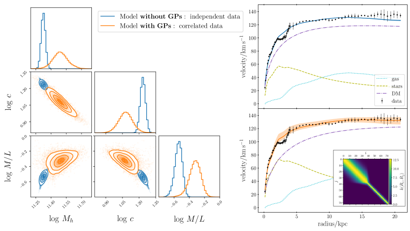
Figure 1: Left-hand panel: marginalized posterior distributions of the model without GPs in blue, assuming independent datapoints, and of the model with GPs in orange, with correlated datapoints. Right-hand panels: rotation curve decompositions of the median blue (top) and orange models (bottom) with a $2-\sigma$ uncertainty band on the predicted $V_{\rm rot}$. The inset in the bottom right panel shows the kernel 4 of the correlation matrix.

3 Conclusions

In this paper I used state-of-the-art observations to show that assuming independent velocity datapoints in rotation curve fits leads to biased parameter constraints and unrealistically small uncertainties on the predicted velocity profile. GPs can be used to account for unknown data correlations with minimal modifications to existing pipelines.

Deriving rotation curves from optical or radio observations is a complex task, unlikely to result in a series of uncorrelated velocity measurements. GPs may provide a simple and computationally cheap solution to use the wealth of literature rotation curve data while accounting for possible underlying correlations.

References

- Aigrain & Foreman-Mackey (2022) Aigrain, S., & Foreman-Mackey, D. 2022, arXiv e-prints, arXiv:2209.08940. https://arxiv.org/abs/2209.08940
- Daigle et al. (2006) Daigle, O., Carignan, C., Amram, P., et al. 2006, MNRAS, 367, 469, doi: 10.1111/j.1365-2966.2006.10002.x
- Foreman-Mackey (2016) Foreman-Mackey, D. 2016, The Journal of Open Source Software, 1, 24, doi: 10.21105/joss.00024
- Foreman-Mackey et al. (2022) Foreman-Mackey, D., Yadav, S., Tronsgaard, R., Schmerler, S., & Theorashid. 2022, dfm/tinygp: tinygp v0.2.2, v0.2.2, Zenodo, Zenodo, doi: 10.5281/zenodo.6473662
- Fraternali et al. (2002) Fraternali, F., van Moorsel, G., Sancisi, R., & Oosterloo, T. 2002, AJ, 123, 3124, doi: 10.1086/340358
- Lelli et al. (2016) Lelli, F., McGaugh, S. S., & Schombert, J. M. 2016, AJ, 152, 157, doi: 10.3847/0004-6256/152/6/157
- Li et al. (2020) Li, P., Lelli, F., McGaugh, S., & Schombert, J. 2020, ApJS, 247, 31, doi: 10.3847/1538-4365/ab700e
- Navarro et al. (1996) Navarro, J. F., Frenk, C. S., & White, S. D. M. 1996, ApJ, 462, 563, doi: 10.1086/177173
- Phan et al. (2019) Phan, D., Pradhan, N., & Jankowiak, M. 2019, arXiv preprint arXiv:1912.11554
- Posti (2022) Posti, L. 2022, lposti/MLPages - Jupyter Notebook: Rotation curve decompositions with Gaussian Processes, v0.1, Zenodo, doi: 10.5281/zenodo.7294885
- Posti et al. (2019) Posti, L., Fraternali, F., & Marasco, A. 2019, A&A, 626, A56, doi: 10.1051/0004-6361/201935553