Parameter Estimation of Two Classes of Nonlinear Systems with Non-separable Nonlinear Parameterizations

Abstract

In this paper we address the challenging problem of designing globally convergent estimators for the parameters of nonlinear systems containing a non-separable exponential nonlinearity. This class of terms appears in many practical applications, and none of the existing parameter estimators is able to deal with them in an efficient way. The proposed estimation procedure is illustrated with two modern applications: fuel cells and human musculoskeletal dynamics. The procedure does not assume that the parameters live in known compact sets, that the nonlinearities satisfy some Lipschitzian properties, nor rely on injection of high-gain or the use of complex, computationally demanding methodologies. Instead, we propose to design a classical on-line estimator whose dynamics is described by an ordinary differential equation given in a compact precise form. A further contribution of the paper is the proof that parameter convergence is guaranteed with the extremely weak interval excitation requirement.

1 Introduction

To comply with the stringent monitoring and control requirements in modern applications an accurate model of the system is vital. It is well-known that nonlinear parameterizations (NLP) are inevitable in any realistic dynamic model of practical problems with complex dynamics. Constitutive relations and conservation equations used to characterize physical variables always involve NLP. Classical examples are friction dynamics (Armstrong-Hélouvry et al., 1994), biochemical processes (Dochain, 2003) and in more recent technological developments we can mention fuel cells (Pukrushpan et al., 2004), photovoltaic arrays (Masters, 2013), windmill generators (Heier, 2014) and biomechanics (Winter, 2009). However, one of the assumptions that pervades almost all results in adaptive estimation and control is linearity in the unknown parameters and there are very few results available for NLP systems. Quite often, in practical problems, there are only few physical parameters that are uncertain and occur nonlinearly in the underlying dynamic model. In some cases, it is possible to use suitable transformations so as to convert it into a problem where the unknown parameters occur linearly, usually involving overparameterizations. This procedure, however, suffers from serious drawbacks including the enlarging of dimension of the parameter space, with the subsequent increase in the excitation requirements needed to ensure parameter convergence. The reader is referred to (Ortega et al., 2020) for a thorough discussion on the drawbacks of overparameterization.

Some results for gradient estimators have been reported in the literature for convexly parameterized systems. It was first reported in (Fomin et al., 1981) (see also (Ortega, 1995)) that convexity is enough to ensure that the gradient search “goes in the right direction” in a certain region of the estimated parameter space. The idea is then to apply a standard adaptive scheme in this region, while in the “bad” region either the adaptation is frozen and a robust constant parameter controller is switched-on (Fradkov et al., 2001) or, as proposed in (Annaswamy et al., 1998), the adaptation is running all the time and stability is ensured with a high-gain mechanism which is suitably adjusted incorporating prior knowledge on the parameters. In (Netto et al., 2000) reparametrization to convexify an otherwise non-convexly parameterized system is proposed. See also (Tyukin et al., 2003, 2007) for some interesting results along these lines, where the controller and the estimator switch between over/underbounding convex/concave functions. Some calculations invoking computationally demanding set membership principles—similar to fuzzy systems—have recently been reported in (Adetola et al., 2014).

Using the Immersion and Invariance adaptation laws proposed in (Astolfi et al., 2008), stronger results were obtained in (Liu et al., 2010, 2011) invoking the property of monotonicity, see also (Tyukin et al., 2003, 2007) for related results. The main advantage of using monotonicity, instead of convexity, is that in the former case the parameter search “goes in the right direction” in all regions of the estimated parameter space—this is in contrast to the convexity-based designs where, as pointed out above, this only happens in some regions of this space. See the recent work (Ortega et al., 2022) where these results relying on monotonicity have been significantly extended. The reader is referred to (Ortega et al., 2020, 2022) for recent reviews of the literature on parameter estimation and adaptive control of NLP systems. Unfortunately, the monotonicity property can be exploited only for the case of separable NLP. That is for the case where we can factor the parameter dependent terms as $h_{i}(u,y,\theta)=\bar{h}_{i}(u,y)\psi_{i}(\theta_{i})$, where $u$ and $y$ are measurable and $\theta_{i}$ is the unknown parameter. However, there are many practical application models where this factorization is not possible, we refer to this case as non-separable NLP. Two often encountered cases are $\cos(\theta_{i}\cdot h_{i}(u,y))$ or $e^{\theta_{i}\cdot h_{i}(u,y)}$. In particular, the last example appears in many physical processes including Arrenhius laws (Silberberg, 2006), biochemical reactors (Dochain, 2003), friction models (Armstrong-Hélouvry et al., 1994), windmill systems (Bobtsov et al., 2022b), fuel cell systems (Xing et al., 2022), photovoltaic arrays (Bobtsov et al., 2022a) and models of elastic moments (Schauer et al., 2005; Sharma et al., 2012; Yang and de Queiroz, 2018). This paper is devoted to the development of a systematic methodology for the parameter identification of systems containing this kind of exponential terms. More precisely, we consider systems of the form

$${\dot{x}=F_{x}(u,y,\theta),y=H_{x}(u,y,\theta)}$$

with $u$ and $y$ measurable and $\theta$ a vector of unknown parameters, with some of its elements entering into the functions $F_{x}$ and/or $H_{x}$ via exponential terms of the form $e^{\theta_{i}\cdot h_{i}(u,y)}$. The objective is to design an on-line estimator

$${\dot{\chi}=F_{\chi}(\chi,u,y),\hat{\theta}=H_{\chi}(\chi,u,y)}$$

with $\chi(t)\in\mathbb{R}^{n_{\chi}}$ such that we ensure global exponential convergence (GEC) of the estimated parameters. That is, for all $x(0)\in\mathbb{R}^{n},\chi(0)\in\mathbb{R}^{n_{\chi}}$ and all continuous $u$ that generates a bounded state trajectory $x$ we ensure

$$\lim_{t\to\infty}|\tilde{\theta}(t)|=0,\quad\mbox{(exp)},$$ (1)

where $\tilde{\theta}:=\hat{\theta}-\theta$ is the parameter estimation error, with all signals remaining bounded.

Notice that, in contrast with the existing approaches for non-separable NLP systems, we do not assume that the parameters live in known compact sets, that the nonlinearities satisfy some Lipschitzian properties, nor rely on injection of high-gain to dominate the nonlinearities or the use of complex, computationally demanding methodologies like min-max optimizations, parameter projections or set membership techniques. Instead, we propose to design a classical on-line estimator whose dynamics is described by an ordinary differential equation given in a compact precise form.

We identify in the paper two classes of systems for which the problem formulated above can be solved. The design procedure consists of the construction—from the non-separable NLP containing an exponential term—a new NLP regression equation (NLPRE) of the form $Y(u,y)=\phi^{\top}(u,y){\mathcal{G}}(\theta)$, where the functions $Y(u,y)$ and $\phi(u,y)$ are known and ${\mathcal{G}}(\theta)$ is a nonlinear mapping. To estimate the parameters $\theta$ from the NLPRE we invoke the recent result of (Ortega et al., 2022), where a least-squares plus dynamic regression equation and mixing (Aranovskiy et al., 2017) (LS+DREM) estimator applicable for this kind of NLPRE is reported. A key feature of the LS+DREM estimator is that it ensures GEC imposing an extremely weak interval excitation (IE) assumption (Kreisselmeier and Rietze-Augst, 1990; Tao, 2003) of the regressor $\phi$. On the other hand, this estimator requires that the mapping of the NLPRE satisfies a rather weak monotonizability property—that is captured by the verifiability of a linear matrix inequality (LMI) imposed on ${\mathcal{G}}(\theta)$. We give two practical examples of the application of the proposed estimation method and illustrate their performance with some simulations.

Notation. $I_{n}$ is the $n\times n$ identity matrix and $0_{s\times r}$ is an $s\times r$ matrix of zeros. $\mathbb{R}_{+}$ and $\mathbb{Z}_{+}$ denote the positive real and integer numbers, respectively. For $q\in\mathbb{Z}_{+}$ we define the set $\bar{q}:=\{1,2,\dots,q\}$. For $a\in\mathbb{R}^{n}$, we denote $|a|^{2}:=a^{\top}a$, and for any matrix $A$ its induced norm is $\|A\|$. All functions and mappings are assumed smooth and all dynamical systems are assumed to be forward complete. Given a function $h:\mathbb{R}^{n}\times\mathbb{R}^{m}\to\mathbb{R}$ we define its transposed gradient via the differential operator $\nabla_{(\cdot)}h(x,u):=\Big{[}\frac{\displaystyle\partial h}{\displaystyle\partial(\cdot)}(x,u)\Big{]}^{\top}$. For a mapping ${\mathcal{G}}:\mathbb{R}^{n_{\eta}}\to\mathbb{R}^{p_{\eta}}$ we denote its Jacobian by $\nabla{\mathcal{G}}(\eta):={\partial{\mathcal{G}}\over\partial\eta}(\eta)$. To simplify the notation, the arguments of all functions and mappings are written only when they are first defined and are omitted in the sequel.

2 First Class of Systems

In this section we consider NLP systems of the form

(2a)

with $x(t)\in{\mathbb{R}^{n}}$, $y(t)\in{\mathbb{R}^{n+1}}$ and $u(t)\in{\mathbb{R}^{m}}$ the systems state, output and control, respectively. The functions $f_{i},\;i=1,2$, and $h_{i},\;i=1,\dots,4$, are known nonlinear functions, ${\mathcal{G}}:\mathbb{R}^{n_{\eta}}\mapsto\mathbb{R}^{p_{\eta}},\;p_{\eta}>n_{\eta}$, is a known mapping of the unknown parameters $\eta\in\mathbb{R}^{n_{\eta}}$, and $\theta_{i}\in\mathbb{R},\;i=1,2$ are also unknown parameters. Hence, the overall vector of unknown parameters, which needs to be estimated on-line, consists of $\theta:=\mbox{col}(\theta_{1},\theta_{2},\eta)\in\mathbb{R}^{\ell_{I}}$, where $\ell_{I}:=2+n_{\eta}$.

We make the important observation that, in view of the presence of the exponential term in the signal $y_{1}$, the parameterization of the system is nonlinear and non-separable. As discussed in the Introduction none of the existing parameter estimators can deal with this difficult—but often encountered in practice—scenario.

2.1 Assumptions

We make the following assumptions on the system.

1. [Sign definiteness] The scalar function $h_{3}$ is bounded away from zero. That is $|h_{3}|>0$.

2. [Monotonicity] There exists a matrix $T_{\mathcal{G}}\in\mathbb{R}^{n_{\eta}\times p_{\eta}}$ such that the mapping ${\mathcal{G}}(\eta)$ satisfies the LMI

   $$T_{\mathcal{G}}\nabla{\mathcal{G}}(\eta)+[\nabla{\mathcal{G}}(\eta)]^{\top}T_{\mathcal{G}}^{\top}\geq\rho_{\mathcal{G}}I_{n_{\eta}},$$ (2c)

   for some $\rho_{\mathcal{G}}{>0}$.

Discussion on the assumptions

D1 In (Ortega et al., 2020, Proposition 1) it is shown that (2g) ensures the mapping $T_{\eta}{\mathcal{G}}(\eta)$ is strictly monotonic (Pavlov et al., 2004). That is, it satisfies

$$(a-b)^{\top}\left[T_{\eta}{\mathcal{G}}(a)-T_{\eta}{\mathcal{G}}(b)\right]\geq\rho_{\eta}|a-b|^{2},\;\forall a,b\in\mathbb{R}^{n_{\eta}},\;a\neq b.$$ (2d)

This is the fundamental property that is required by the LS+DREM estimator used in the next section.

D2 The assumption that the state trajectories of (2) are bounded is standard in parameter estimation theory (Ljung, 1987; Sastry and Bodson, 1989). Similarly, the assumption that the dimension $n_{\eta}$ of the unknown parameters vector $\eta$ is smaller than $p_{\eta}$ is reasonable, otherwise we could redefine a new vector of unknown parameters $\bar{\eta}:={\mathcal{G}}(\eta)\in\mathbb{R}^{n_{\eta}}$ without overparameterization and get a LRE.

2.2 Regression Equation for Parameter Estimation

In this section derive the regression equation that will be used to estimate the unknown parameters $\theta$. As expected, this regressor equation is nonlinearly parameterized, which hampers the application of standard estimation techniques. Therefore, we are compelled to appeal—in Section LABEL:sec4—to the LS+DREM parameter estimator recently reported in (Ortega et al., 2022; Pyrkin et al., 2022).

Lemma 1

Consider the system (2) verifying Assumptions A1, A2. There exists measurable, scalar signals $Y_{I}(x,u,y),\;\phi_{I,i}(x,u,y),\;i=1,\dots,s_{I},\;s_{I}:=3+2p_{\eta},$ such that the following NLPRE holds:

$$Y_{I}(x,u,y)=\phi_{I}^{\top}(x,u,y){\mathcal{W}}_{I}(\theta),$$ (2e)

where we defined the mapping ${\mathcal{W}}_{I}:\mathbb{R}^{\ell_{I}}\to\mathbb{R}^{s_{I}}$

$${\mathcal{W}}_{I}(\theta):=\begin{bmatrix}\theta_{1}&\theta_{2}&\theta_{1}\theta_{2}&\theta_{1}{\mathcal{G}}^{\top}(\eta)&\theta_{1}\theta_{2}{\mathcal{G}}^{\top}(\eta)\end{bmatrix}^{\top}.$$ (2f)

Discussion on the regressor equation

D3 It is possible to construct another NLPRE proceeding as follows. First, exploiting the monotonicity property of Assumption A2 and using the LS+DREM algorithm estimate the parameters $\eta$ filtering (2a). Then, use this estimate in the (approximate) calculation of $\dot{h}_{4}$, yielding

$$\dot{\hat{h}}_{4}=\nabla^{\top}h_{4}[f_{1}+f_{2}{\mathcal{G}}(\hat{\eta})].$$

Applying the certainty equivalent principle, and replacing this expression in the chain of implications of the proof of Lemma 1 in Appendix A would then yield a simpler NLPRE where only the terms $(\theta_{1},\theta_{2},\theta_{1}\theta_{2})$ will appear. Of course, the drawback of this approach is that we rely on the fast convergence of $\tilde{\eta}:=\hat{\eta}-\eta$ to zero.

D4 In the system (2) the function $h_{4}$ appearing in the exponential does not depend on $u$. It is possible to adapt the result of Lemma 1 to consider that case in the following way. The expression for $\dot{h}_{4}$ given in (2hp) would need to be replaced by

$$\dot{h}_{4}=\nabla_{x}^{\top}h_{4}[f_{1}+f_{2}{\mathcal{G}}(\eta)]+\nabla_{u}^{\top}h_{4}\dot{u}.$$

To construct the NPLRE as in Lemma 1 for this case it is clearly necessary to know $\dot{u}$. However, in many practical applications the control law contains an integral action—e.g., in PID control—therefore this signal is available for measurement.

2.3 Construction of a Strictly Monotonic Mapping

To estimate the parameters $\theta$ from the NLPRE (2e) we invoke the recent result of (Ortega et al., 2022), where the LS+DREM estimator proposed in (Pyrkin et al., 2022), which is applicable for linear regression equations, was extended to deal with NLPRE. However, this estimator requires that the mapping of the NLPRE satisfies a monotonicity property, which is not verified by ${\mathcal{W}}_{I}(\theta)$ given in (2f). Therefore, in this section we construct a new mapping verifying the required monotonicity condition.

Lemma 2

Consider the mapping ${\mathcal{W}}(\theta)$ given in (2f) with ${\mathcal{G}}(\eta)$ verifying Assumption A2. There exists a constant $\alpha_{m}>0$ such that for all $\alpha\geq\alpha_{m}$ the mapping ${\mathcal{W}}_{I}(\theta)$ satisfies the LMI

$$T_{{\mathcal{W}}_{I}}\nabla{\mathcal{W}}_{I}(\theta)+[\nabla{\mathcal{W}}_{I}(\theta)]^{\top}T_{{\mathcal{W}}_{I}}^{\top}\geq\rho_{{\mathcal{W}}_{I}}I_{\ell_{I}},$$ (2g)

for some $\rho_{{\mathcal{W}}_{I}}>0$, with the matrix

$$T_{{\mathcal{W}}_{I}}:=\begin{bmatrix}\alpha&0&0&0_{1\times p_{\eta}}&0_{1\times p_{\eta}}\\ 0&\alpha&0&0_{1\times p_{\eta}}&0_{1\times p_{\eta}}\\ &0_{n_{\eta}\times 3}&&\emph{sign}(\theta_{1})T_{\mathcal{G}}&0_{n_{\eta}\times p_{\eta}}\end{bmatrix}\in\mathbb{R}^{\ell_{I}\times s_{I}}.$$

Discussion on the mapping

D5 Notice that the only prior knowledge needed to construct the matrix $T_{{\mathcal{W}}_{I}}$ is $\mbox{sign}(\theta_{1})$. On the other hand, to select the value of $\alpha$ some prior knowledge on the parameters $\theta$ is required. Specifically, as shown in the proof of Lemma 2 in Appendix A, it is necessary to know an upper bound on $\|T_{\mathcal{G}}{\mathcal{G}}(\eta)\|$.

3 Second Class of Systems

In this section we consider second order systems of the form

A4 [Excitation] The regressor vector $\phi$ is IE. That is, there exist constants $C_{c}>0$ and $t_{c}>0$ such that

$$\int_{0}^{t_{c}}\phi(s)\phi^{\top}(s)ds\geq C_{c}I_{s}.$$

The proof of the proposition below is given in (Ortega et al., 2022, Proposition 1), therefore it is omitted here.

Proposition 1

Consider the NLPRE (LABEL:nlpre) with $\phi$ verifying Assumption A4 and ${\mathcal{W}}$ satisfying the LMI

$$T_{{\mathcal{W}}}\nabla{\mathcal{W}}(\theta)+[\nabla{\mathcal{W}}(\theta)]^{\top}T_{{\mathcal{W}}}^{\top}\geq\rho_{{\mathcal{W}}}I_{\ell}$$

for some matrix $T_{{\mathcal{W}}}\in\mathbb{R}^{\ell\times s}$ and $\rho_{{\mathcal{W}}}>0$. Define the LS+DREM interlaced estimator

with tuning gains the scalars $\gamma_{\mathcal{W}}>0$, $f_{0}>0$ and the positive definite matrix $\Gamma\in\mathbb{R}^{\ell\times\ell}$, and we defined the signals

$${\Delta:=\det\{I_{s}-f_{0}F\},{\mathcal{Y}}:=\emph{\mbox{adj}}\{I_{s}-f_{0}F\}(\hat{\mathcal{W}}-f_{0}F{\mathcal{W}}_{0}),}$$

where $\emph{adj}\{\cdot\}$ denotes the adjugate matrix. For all initial conditions ${\mathcal{W}}_{0}\in\mathbb{R}^{s}$ and $\theta_{0}\in\mathbb{R}^{\ell}$. The estimation errors of the parameters $\tilde{\theta}$ verify (1) with all signals bounded.

5 Two Practical Examples

5.1 Proton Exchange Membrane Fuel Cell

Parameter estimation is vital for modeling and control of fuel cell systems. However, an accurate description of the fuel cell dynamics implies the use of models with nonlinear parameterizations (Pukrushpan et al., 2004). The interested reader is refered to (Xing et al., 2022) where a detailed review of the literature on parameter estimation of fuel cell systems is reported.

Verification of the conditions from the general result

A widely accepted mathematical model of a Proton Exchange Membrane Fuel Cell (PEMFC) is given in (Xing et al., 2022, Section II.B). It can be shown that this model can be written in the form (2) with $n=m=n_{\eta}=p_{\eta}=1$ and the scalar linear map ${\mathcal{G}}(\eta)=\eta$.

We make the observation that function $h_{3}$, which is proportional to the membrane conductivity, is bounded away from zero, hence verifying Assumption A1.

Since ${\mathcal{G}}=\theta_{3}$ the mapping ${\mathcal{W}}_{I}:\mathbb{R}^{3}\to\mathbb{R}^{5}$ defined in (2f) is simpler and given as

$${\mathcal{W}}_{I}(\theta):=\begin{bmatrix}\theta_{1}&\theta_{2}&\theta_{1}\theta_{2}&\theta_{1}\theta_{3}&\theta_{1}\theta_{2}\theta_{3}\end{bmatrix}^{\top}.$$

Some simple calculations give us terms $Y_{I}$ and $\phi_{I}^{\top}$ for the NLPRE (2e). And the matrix $T_{{\mathcal{W}}_{I}}$ of Lemma 2 is given as

$$T_{{\mathcal{W}}_{I}}:=\begin{bmatrix}\alpha&0&0&0&0\\ 0&\alpha&0&0&0\\ 0&0&0&\mbox{sign}(\theta_{1})&0\end{bmatrix},$$

and the minimum value for $\alpha$ is $\alpha_{m}={\theta^{2}_{3}\over|\theta_{1}|}.$

5.2 Human Shank Dynamics

Neuromuscular electrical stimulation is an active research area that aims at restoring functionality to human limbs with motor neuron disorders. Control of these systems is a challenging problem because the musculoskeletal dynamics are nonlinear and highly uncertain (Winter, 2009). In this subsection we are interested in the mechanical dynamics of the human shank motion where the input is the joint torque produced by electrode stimulation of the shank muscles. We consider the scenario described in detail in (Yang and de Queiroz, 2018), see also (Schauer et al., 2005; Sharma et al., 2012) and concentrate our attention on the problem of estimating the parameters of a widely accepted mathematical model of this system. Namely, the system described by equations (11) to (14) of (Yang and de Queiroz, 2018), that we repeat here for ease of reference

$$J\ddot{x}+b_{1}\dot{q}+b_{2}\mbox{sign}(\dot{x})+k_{1}e^{-k_{2}x}(x-q_{0})+mg\ell\sin(x)=u,$$ (2hm)

where $(x,\dot{x})$ are assumed measurable and all the parameters are assumed unknown. The reader is referred to this reference for further details on the model, in particular, the physical interpretation of the different terms in the model, and the overall formulation of the neuromuscular electrical stimulation problem.

Verification of the conditions from the general result

The following clarifications regarding our formulation of the parameter estimation problem are in order.

• As indicated in (Yang and de Queiroz, 2018), the term $\mbox{sign}(\dot{x})$ of our model (2hm) is replaced in equation (12) of (Yang and de Queiroz, 2018) by the function $\tanh(b_{3}\dot{x})$, with a large value for $b_{3}>0$, which is a smooth approximation of the sign function. This approximation is made for mathematical convenience of their calculations that rely on a smoothness assumption, but is not required in our approach that can deal with discontinuous nonlinearities.

• In this paper we assume that the term $q_{0}$, which is the constant resting knee angle, and the constant inertia $J$ are known. Therefore the uncertain parameters in our case are $\mbox{col}(b_{1},b_{2},k_{1},k_{2},m\ell)$. The assumption of known $J$ is not to restrictive because the inertia can be predicted from the subject’s anthropometric data (Winter, 2009).

• In (Yang and de Queiroz, 2018) there is an additional, bounded, unstructured, additive term in (2hm) that is omitted here for brevity. As shown in Proposition 1 we achieve GEC of the parameter estimates, therefore this term could be easily accommodated in our analysis to ensure practical stability.

The dynamics (2hm) belongs to the second class of systems given by (2h) with $n_{\eta}=p_{\eta}=3$, and the following definitions for the functions and the parameters

$${&\theta_{1}=k_{2},\;{\mathcal{G}}(\eta)=\eta=\mbox{col}(b_{1},b_{2},m\ell),\;\theta:=\mbox{col}(\theta_{1},\eta^{\top}).}$$

We bring to the readers attention the fact that the model (2hm) has a parameter $k_{1}$ multiplying the exponential term. Therefore, it is necessary to invoke the two-stage certainty-equivalent based procedure described in Discussion D7. That is, we estimate with the NLPRE (LABEL:nlpre2) the parameters $(k_{2},b_{1},b_{2},m\ell)$ and then estimate, e.g., with some filtering and a standard gradient, the remaining parameter $k_{1}$.

To comply with Assumption A1, we assume that $|x-q_{0}|>0$. Clearly, since ${\mathcal{G}}(\eta)=\eta$, Assumption A2 is satisfied with $T_{{\mathcal{G}}}={\rho_{\mathcal{G}}\over 2}I_{3}$, with any $\rho_{\mathcal{G}}>0$. Finally Assumption A3 is satisfied with the functions

$$\psi_{a}(x):=\begin{bmatrix}-1&0&0\\ 0&-1&0\\ 0&0&g\sin(x)\end{bmatrix},\;\psi_{b}(\dot{x}):=\begin{bmatrix}\dot{x}\\ \mbox{sign}(\dot{x})\\ 1\end{bmatrix}.$$

The mapping ${\mathcal{W}}_{II}:\mathbb{R}^{4}\to\mathbb{R}^{7}$ is given as

$${\mathcal{W}}_{II}(\theta):=\begin{bmatrix}k_{2}&b_{1}&b_{2}&m\ell&k_{2}b_{1}&k_{2}b_{2}&k_{2}m\ell\end{bmatrix}^{\top}.$$

Some simple calculations give us terms $Y_{II}$ and $\phi_{II}^{\top}$ for the NLPRE (LABEL:nlpre2).

Finally, the matrix $T_{{\mathcal{W}}_{II}}\in\mathbb{R}^{4\times 7}$ of Lemma LABEL:lem4 is given as

$$T_{{\mathcal{W}}_{II}}:=\begin{bmatrix}1&0&0&0&0&0&0\\ 0&{\rho_{\mathcal{G}}\over 2}&0&0&0&0&0\\ 0&0&{\rho_{\mathcal{G}}\over 2}&0&0&0&0\\ 0&0&0&{\rho_{\mathcal{G}}\over 2}&0&0&0\end{bmatrix}.$$

6 Simulation Results

6.1 First class of systems

Consider the ”synthetic” model of the first slass of the systems in the form (2), where $f_{1}=-x+u$, $f_{2}=u$, $h_{1}=x^{2}$, $h_{2}=x-353$, $h_{3}=0.1+x^{2}$, $h4=-1/x$.

Since ${\mathcal{G}}=\theta_{3}$ the mapping ${\mathcal{W}}_{I}:\mathbb{R}^{3}\to\mathbb{R}^{5}$ defined in (2f) is simpler and given as

$${\mathcal{W}}_{I}(\theta):=\begin{bmatrix}\theta_{1}&\theta_{2}&\theta_{1}\theta_{2}&\theta_{1}\theta_{3}&\theta_{1}\theta_{2}\theta_{3}\end{bmatrix}^{\top}.$$

Some simple calculations show that the terms of the NLPRE (2e) are given as

For simulations we used next parameter values: filters parameter $\lambda=600$, $\hat{{\mathcal{W}}}(0)=[0\;0\;0\;0\;0]$, $f_{0}=1$, $\hat{\theta}=col[0\;0\;0]$, $\Gamma=10^{3}\begin{bmatrix}&1&0&0\\ &0&1&0\\ &0&0&1\end{bmatrix}$, $T_{{\mathcal{W}}}=\begin{bmatrix}&10&0&0&0&0\\ &0&10&0&0&0\\ &0&0&0&10&0\end{bmatrix}$.

Fig. 1 … Fig. 3 demonstrate error transients of parameter estimations. In simulations we swithed on our observer on the fifth second. Figures demonstrate that error transients tends to the zero.

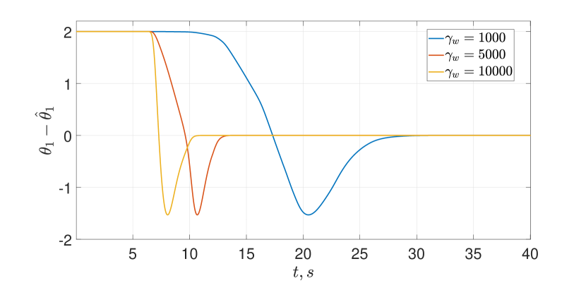
Figure 1: Transients of the error $\theta_{1}-\hat{\theta}_{1}$ for different values of the parameter $\gamma_{w}$

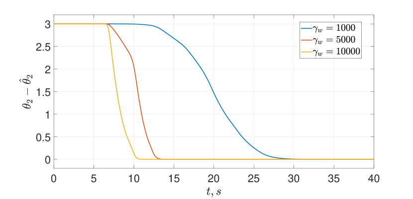
Figure 2: Transients of the error $\theta_{2}-\hat{\theta}_{2}$ for different values of the parameter $\gamma_{w}$

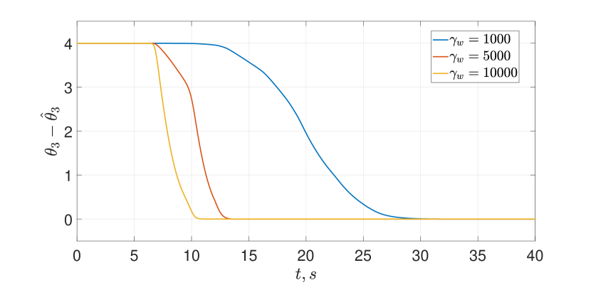
Figure 3: Transients of the error $\theta_{3}-\hat{\theta}_{3}$ for different values of the parameter $\gamma_{w}$

6.2 Second class of systems

Parameters of the human shank model were chosen as in (Yang and de Queiroz, 2018). For estimation of shank model parameters we used algorithm from proposition 1 with $\hat{{\mathcal{W}}}(0)=[0\;0\;0\;0\;0\;0\;0]$, $f_{0}=10^{-3}$, $\Gamma=\begin{bmatrix}&1&0&0&0\\ &0&1&0&0\\ &0&0&1&0\\ &0&0&0&1\end{bmatrix}$, $T_{{\mathcal{W}}}=\begin{bmatrix}&1&0&0&0&0&0&0\\ &0&1&0&0&0&0&0\\ &0&0&1&0&0&0&0\\ &0&0&0&1&0&0&0\end{bmatrix}$, $\hat{\theta}=col[0\;0\;0\;0\;0\;0\;0]$ and $\lambda=1$ in the filters.

Consider computer simulations of human shank system with dynamic robust control from (Yang and de Queiroz, 2018)

$$u(t)=(k_{1}+1)r(t)-(k_{1}+1)r(0)+$$

$$+\int\limits_{0}^{t}\left[(k_{1}+1)k_{2}r(\tau)+k_{3}sign(r(\tau))\right]d\tau$$

where $e=x-x$ and $r=\dot{e}-\mu e$. For simulation we used $\dot{x}_{1}=\begin{bmatrix}&0&1&0\\ &0&0&1\\ &-6000&-1300&-80\end{bmatrix}x_{1}+\begin{bmatrix}0\\ 0;\\ 1\end{bmatrix}w$,

$$\left\{\begin{matrix}&1000\pi/3,&0\leqslant t<20s,\\ &1000\pi,&10\leqslant t<40s,\\ &2500\pi,&t\geqslant 40s,\end{matrix}\right.$$ (2hn)

$x_{1}=[x_{d}\;\dot{x}_{d}\;\ddot{x}_{d}]^{\top}$.

For simulation we used $\mu=4$, $k_{1}=1$, $k_{2}=2$ and $k_{3}=40$ for control algorithm (simulation results for Human Shank with control are shown on Fig. 4 and Fig. 5) and $\lambda=10$, $\gamma=10^{6}$, $\Gamma=10^{5}I$, $f_{0}=0.001$.

Fig. 4 demonstrates transient of the system output $x$. Fig. 5 demonstrates transient of the error $x-x_{d}$. Fig. 6…9 demonstrate transients of estimation errors.

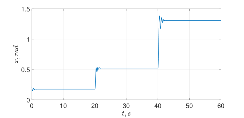
Figure 4: Transient of the output $x$

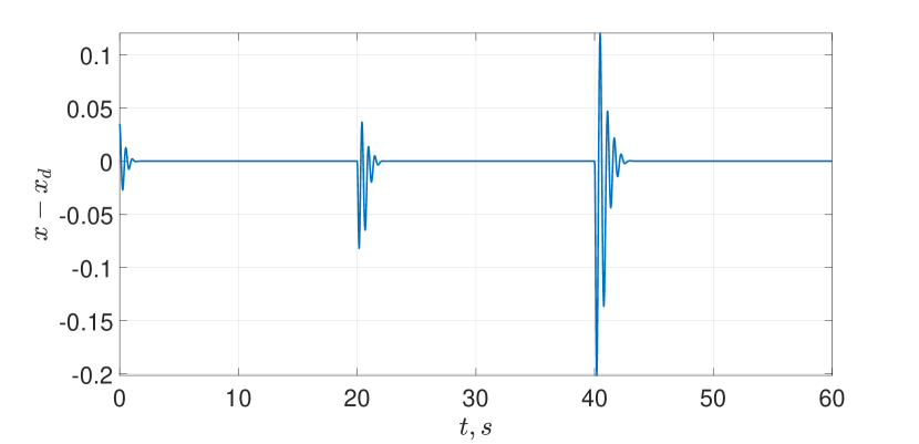
Figure 5: Transients of the error $x-x_{d}$

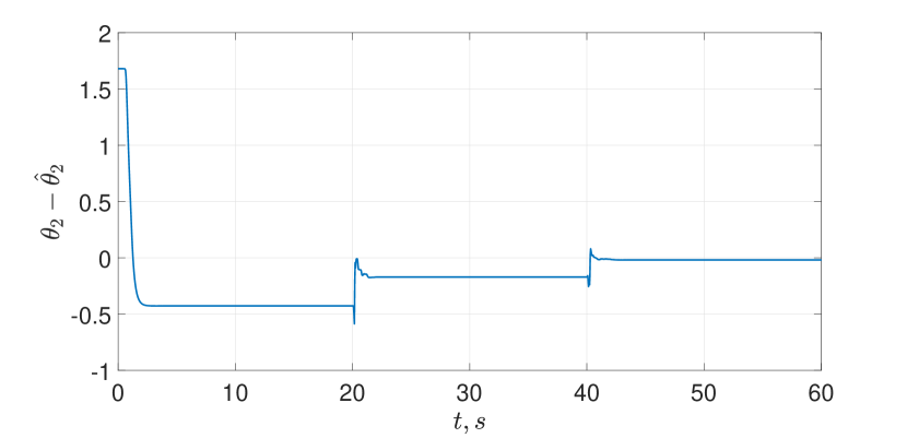
Figure 6: Transients of the error $\theta_{2}-\hat{\theta}_{2}$ ($k_{2}-\hat{k}_{2}$)

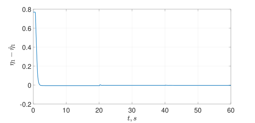
Figure 7: Transients of the error $\eta_{1}-\hat{\eta}_{1}$ ($\frac{b_{1}}{J}-\widehat{\frac{b_{1}}{J}}$)

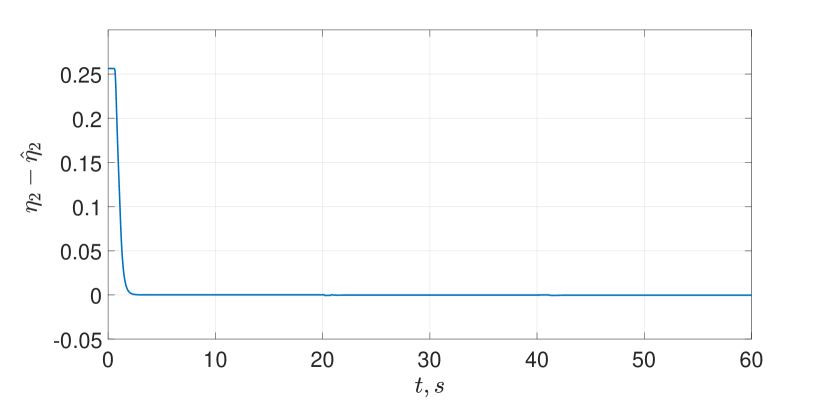
Figure 8: Transients of the error $\eta_{2}-\hat{\eta}_{2}$ ($\frac{b_{2}}{J}-\widehat{\frac{b_{2}}{J}}$)

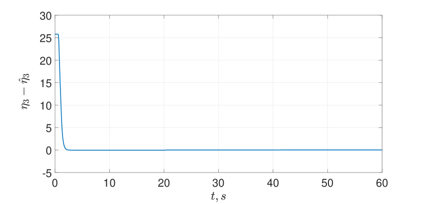
Figure 9: Transients of the error $\eta_{3}-\hat{\eta}_{3}$ ($\frac{mgl}{J}-\widehat{\frac{mgl}{J}}$)

If parameters $\theta_{2}$ and $\eta$ are known then we can estimate parameter $\theta_{1}$ using for instance standard gradietnt observer. We found paramete $\theta_{1}$ with standard gradient observer using $\theta_{2}$ and $\hat{\eta}$ instead real values with adaptation gain $10^{6}$ (see simulation result on the Fig. 10).

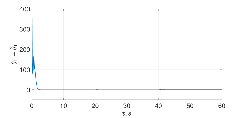
Figure 10: Transients of the error $\theta_{1}-\hat{\theta}_{1}$ ($\frac{k_{1}}{J}-\widehat{\frac{k_{1}}{J}}$)

Simulation results demonstrate convergence estimates to real values.

7 Concluding Remarks

We have presented in this paper a constructive procedure to design GEC estimators for the parameters of two classes of nonlinear, NLP systems containing nonseparable nonlinearities of the form $e^{\theta_{i}h_{i}(u,y)}$. Although this class of nonlinearities seems to be very particular, as discussed in the Introduction, it appears in many practical applications, including the two thoroughly studied in the paper, and is not amenable for the application of the existing parameter estimation techniques. The design procedure consists of the construction—from the non-separable NLP containing the exponential term—a new separable NLPRE, for which we can apply the LS+DREM estimator of (Ortega et al., 2022). It is important to underscore that, to the best of our knowledge, only this estimator is capable of dealing with this kind of NLPREs. Moreover, the excitation requirement needed to ensure GEC is the very weak condition of IE defined in Assumption A4.

We would like to bring to the readers attention that techniques similar to the ones proposed here have been recently applied by the authors to solve two currently very relevant practical applications. Indeed, in (Bobtsov et al., 2022b) we solve the problem of estimation of the parameters of the power coefficient of windmill generators in off-grid operation. The mathematical model of this system is of the form

$$\dot{y}=-y^{3}(\theta_{1}y-\theta_{2})e^{-\theta_{3}y},$$

with $\theta\in\mathbb{R}^{3}$ unknown parameters. Also, in (Bobtsov et al., 2022a) we proposed a GEC parameter estimator for photo-voltaic arrays, whose dynamic model is of the form

$${\dot{x}=-\theta_{1}x-\theta_{2}e^{bx}+\theta_{3}-\theta_{4}u,y=x-\theta_{5}u,}$$

with $\theta\in\mathbb{R}^{5}$ unknown parameters, and the state $x(t)\in\mathbb{R}$ unmeasurable. Notice that none of these applications fits into the class of systems considered in the paper.

Appendix A Proof of Lemmas

Proof of Lemma 1

We make the key observation that the function $h_{4}$ verifies

$$\dot{h}_{4}=\nabla^{\top}h_{4}[f_{1}+f_{2}{\mathcal{G}}(\eta)],$$

where we have used (2a).

To simplify the notation in the sequel we define

$$h_{5}:=\nabla^{\top}h_{4}f_{1},\;h_{6}:=f_{2}^{\top}\nabla h_{4},\;h_{7}:={y_{1}-h_{1}\over h_{3}},\;h_{8}:=-{h_{2}\over h_{3}}.$$ (2ho)

We observe that using this notation we can write

$$\dot{h}_{4}=h_{5}+h^{\top}_{6}{\mathcal{G}}(\eta).$$ (2hp)

From the definition of $y_{1}$ in (LABEL:y1) we get

$${e^{h_{4}\theta_{1}}=h_{7}+h_{8}\theta_{2}\mathrel{\overset{\makebox[0.0pt]{\mbox{\tiny${d\over dt}$}}}{\Longrightarrow}}\theta_{1}\dot{h}_{4}e^{h_{4}\theta_{1}}=\dot{h}_{7}+\dot{h}_{8}\theta_{2}}$$

$${\mathrel{\overset{\makebox[0.0pt]{\mbox{\tiny${d\over dt}$}}}{\Longrightarrow}}\theta_{1}\dot{h}_{4}e^{h_{4}\theta_{1}}=\dot{h}_{7}+\dot{h}_{8}\theta_{2}}$$

$${\Longleftrightarrow\theta_{1}\dot{h}_{4}(h_{7}+h_{8}\theta_{2})=\dot{h}_{7}+\dot{h}_{8}\theta_{2}}$$

$${\Longleftrightarrow\dot{h}_{7}=\dot{h}_{4}h_{7}\theta_{1}+\dot{h}_{4}h_{8}\theta_{1}\theta_{2}-\dot{h}_{8}\theta_{2}}$$

$${\Longrightarrow\dot{h}_{7}=[h_{5}+h^{\top}_{6}{\mathcal{G}}(\eta)]h_{7}\theta_{1}+[h_{5}+h^{\top}_{6}{\mathcal{G}}(\eta)]h_{8}\theta_{1}\theta_{2}}$$

$${-\dot{h}_{8}\theta_{2}}$$

$${\Longleftrightarrow\dot{h}_{7}=\theta_{1}h_{5}h_{7}-\theta_{2}\dot{h}_{8}+\theta_{1}\theta_{2}h_{5}h_{8}+\theta_{1}{\mathcal{G}}^{\top}(\eta)h_{7}h_{6}}$$

$${+\theta_{1}\theta_{2}{\mathcal{G}}^{\top}(\eta)h_{8}h_{6},}$$

where we used (2hp) to get the fourth implication. To obtain from the last identity a measurable NLPRE we apply the standard filtering technique (Jing and Ioannou, 1996; Tao, 2003). Toward this end, we fix a constant $\lambda>0$ and define the stable filter ${\lambda\over p+\lambda}$, where $p:={d\over dt}$. Applying this filter to the last equation above, and recalling the definitions (2ho), we get appropriate vectors $Y_{I}$ and $\phi_{I}$ for the NLPRE (2e) completing the proof.

Proof of Lemma 2

The Jacobian of ${\mathcal{W}}(\theta)$ is given as

$$\nabla{\mathcal{W}}(\theta)=\begin{bmatrix}1&0&0_{1\times n_{\eta}}\\ 0&1&0_{1\times n_{\eta}}\\ \theta_{2}&\theta_{1}&0_{1\times n_{\eta}}\\ {\mathcal{G}}(\eta)&0_{p_{\eta}\times 1}&\theta_{1}\nabla{\mathcal{G}}(\eta)\\ \theta_{2}{\mathcal{G}}(\eta)&\theta_{1}{\mathcal{G}}(\eta)&\theta_{1}\theta_{2}\nabla{\mathcal{G}}(\eta)\end{bmatrix}.$$

The symmetric part of the matrix $T_{\mathcal{W}}\nabla{\mathcal{W}}(\theta)$ takes the form

Let us introduce the notation

$${B:=\begin{bmatrix}\mbox{sign}(\theta_{1}){\mathcal{G}}^{\top}(\eta)T_{\mathcal{G}}^{\top}\\ \cdots\\ 0_{1\times n_{\eta}}\end{bmatrix},}$$

$${C:=|\theta_{1}|\{T_{\mathcal{G}}\nabla{\mathcal{G}}(\eta)+[\nabla{\mathcal{G}}(\eta)]^{\top}T_{\mathcal{G}}^{\top}\}.}$$

A simple Schur complement calculation proves that the matrix $T_{\mathcal{W}}{\nabla}{\mathcal{W}}(\theta)+[\nabla{\mathcal{W}}(\theta)]^{\top}T_{\mathcal{W}}^{\top}$ is positive definite if and only if

$$C>{1\over 2\alpha}B^{\top}B.$$ (2hq)

On the other hand, from Assumption A3 we have that $C\geq|\theta_{1}|\rho_{\mathcal{G}}I_{n_{\eta}}>0$. From which we conclude that (2hq) holds for sufficiently large $\alpha$, concluding the proof.

Proof of Lemma LABEL:lem3

To simplify the notation in the sequel we define

$$f_{3}:={f_{1}\over h_{3}},\;f_{4}:={1\over h_{3}}f_{2}.$$ (2hr)

We observe that using this notation and (2h) we get the following chain of implications

$${{1\over h_{3}}\ddot{x}=e^{h_{4}\theta_{1}}+f_{3}+f^{\top}_{4}{\mathcal{G}}(\eta)+{u\over h_{3}}}$$

$${\mathrel{\overset{\makebox[0.0pt]{\mbox{\tiny${d\over dt}$}}}{\Longrightarrow}}-{\dot{h}_{3}\over h^{2}_{3}}\ddot{x}+{1\over h_{3}}{d^{3}x\over dt^{3}}=\theta_{1}\dot{h}_{4}\Big{(}e^{h_{4}\theta_{1}}\Big{)}+\dot{f}_{3}+\dot{f}^{\top}_{4}{\mathcal{G}}(\eta)}$$

$${-{\dot{h}_{3}\over h^{2}_{3}}u+{\dot{u}\over h_{3}}}$$

$${\Longleftrightarrow-{\dot{h}_{3}\over h^{2}_{3}}\ddot{x}+{1\over h_{3}}{d^{3}x\over dt^{3}}=\theta_{1}\dot{h}_{4}\Big{(}{1\over h_{3}}\ddot{x}-f_{3}-f^{\top}_{4}{\mathcal{G}}(\eta)-{u\over h_{3}}\Big{)}}$$

$${+\dot{f}_{3}+\dot{f}^{\top}_{4}{\mathcal{G}}(\eta)-{\dot{h}_{3}\over h^{2}_{3}}u+{\dot{u}\over h_{3}}}$$

$${\mathrel{\overset{\makebox[0.0pt]{\mbox{\tiny$\times h_{3}$}}}{\Longrightarrow}}-{\dot{h}_{3}\over h_{3}}\ddot{x}+{d^{3}x\over dt^{3}}=\theta_{1}\dot{h}_{4}\Big{(}\ddot{x}-h_{3}f_{3}-h_{3}f^{\top}_{4}{\mathcal{G}}(\eta)-u\Big{)}}$$

$${&+h_{3}\dot{f}_{3}+h_{3}\dot{f}^{\top}_{4}{\mathcal{G}}(\eta)-{\dot{h}_{3}\over h_{3}}u+\dot{u}.}$$

Moving to the left hand side the term which are independent of the unknown parameters we obtain the key identity

To obtain from (LABEL:keyide) a measurable NLPRE we apply the standard filtering technique with the stable second order filter ${\lambda^{2}\over(p+\lambda)^{2}}$. We observe that, due to the measurement of $\dot{x}$, the term

$${\lambda^{2}\over(p+\lambda)^{2}}{d^{3}x\over dt^{3}}={\lambda^{2}p^{2}\over(p+\lambda)^{2}}\dot{x},$$

is computable without differentiation. The same argument can be applied to all the other terms, except ${\dot{h}_{3}\over h_{3}}\ddot{x}$, $\dot{h}_{4}\ddot{x}$ and $h_{3}\dot{f}_{4}$, which involve the unmeasurable signal $\ddot{x}$. To overcome this problem we invoke the Swapping Lemma (Sastry and Bodson, 1989, Lemma 3.6.5)

where the last right hand term can be computed without differentiation. Clearly, the same procedure can be applied to the term ${\dot{h}_{3}\over h_{3}}\ddot{x}$, leading to

where, again, the last right hand term can be computed without differentiation.

Now, regarding the term $h_{3}\dot{f}_{4}$, from (2hr), we have that

where we used Assumption A3 in the third identity and defined the function $\psi_{c}:=\int\psi_{b}(s)ds$. Applying the Swapping Lemma we can take care of the term $\psi_{a}\dot{\psi}_{c}$

which is clearly computable.

Applying the second order filter to (LABEL:keyide) and invoking the calculations above we get, after lengthy but straightforward calculations, get appropriate vectors $Y_{II}$ and $\phi_{II}$ for the NLPRE (LABEL:nlpre2) completing the proof.

References

- Adetola et al. (2014) Adetola, V., Guay, M., and Lehrer, D. (2014). Adaptive estimation for a class of nonlinearly parameterized dynamical systems. IEEE Transactions on Automatic Control, 59(10), 2818–2824. 10.1109/TAC.2014.2318080.
- Annaswamy et al. (1998) Annaswamy, A.M., Skantze, F.P., and Loh, A.P. (1998). Adaptive control of continuous time systems with convex/concave parametrization. Automatica, 34(1), 33–49. https://doi.org/10.1016/S0005-1098(97)00159-3.
- Aranovskiy et al. (2017) Aranovskiy, S., Bobtsov, A., Ortega, R., and Pyrkin, A. (2017). Performance enhancement of parameter estimators via dynamic regressor extension and mixing. IEEE Transactions on Automatic Control, 62(7), 3546–3550. 10.1109/TAC.2016.2614889.
- Armstrong-Hélouvry et al. (1994) Armstrong-Hélouvry, B., Dupont, P., and De Wit, C.C. (1994). A survey of models, analysis tools and compensation methods for the control of machines with friction. Automatica, 30(7), 1083–1138. https://doi.org/10.1016/0005-1098(94)90209-7.
- Astolfi et al. (2008) Astolfi, A., Karagiannis, D., and Ortega, R. (2008). Nonlinear and adaptive control with applications, volume 187. Springer. https://doi.org/10.1007/978-1-84800-066-7.
- Bobtsov et al. (2022a) Bobtsov, A., Mancilla-David, F., Aranovskiy, S., and Ortega, R. (2022a). On-line identification of photovoltaic arrays’ dynamic model parameters. Automatica, (submitted), arXiv preprint arXiv:2209.07246.
- Bobtsov et al. (2022b) Bobtsov, A., Ortega, R., Aranovskiy, S., and Cisneros, R. (2022b). On-line estimation of the parameters of the windmill power coefficient. Systems & Control Letters, 164, 105242.
- Dochain (2003) Dochain, D. (2003). State and parameter estimation in chemical and biochemical processes: a tutorial. Journal of Process Control, 13(8), 801–818. https://doi.org/10.1016/S0959-1524(03)00026-X.
- Fomin et al. (1981) Fomin, V., Fradkov, A., and Yakubovich, V. (1981). Adaptive control of dynamical systems. Nauka, Moskow, in Russian.
- Fradkov et al. (2001) Fradkov, A., Ortega, R., and Bastin, G. (2001). Semi-adaptive control of convexly parametrized systems with application to temperature regulation of chemical reactors. International Journal of Adaptive Control and Signal Processing, 15(4), 415–426. https://doi.org/10.1002/acs.634.
- Heier (2014) Heier, S. (2014). Grid integration of wind energy: onshore and offshore conversion systems. John Wiley & Sons.
- Jing and Ioannou (1996) Jing, S. and Ioannou, P. (1996). Robust Adaptive Control. Prentice-Hall, New Jersey.
- Kreisselmeier and Rietze-Augst (1990) Kreisselmeier, G. and Rietze-Augst, G. (1990). Richness and excitation on an interval-with application to continuous-time adaptive control. IEEE Transactions on Automatic Control, 35(2), 165–171. 10.1109/9.45172.
- Liu et al. (2010) Liu, X., Ortega, R., Su, H., and Chu, J. (2010). Immersion and invariance adaptive control of nonlinearly parameterized nonlinear systems. IEEE Transactions on Automatic Control, 55(9), 2209–2214. 10.1109/TAC.2010.2052389.
- Liu et al. (2011) Liu, X., Ortega, R., Su, H., and Chu, J. (2011). On adaptive control of nonlinearly parameterized nonlinear systems: Towards a constructive procedure. Systems & Control Letters, 60(1), 36–43. https://doi.org/10.1016/j.sysconle.2010.10.004.
- Ljung (1987) Ljung, L. (1987). System Identification: Theory for the user. Prentice Hall, New Jersey.
- Masters (2013) Masters, G.M. (2013). Renewable and efficient electric power systems. John Wiley & Sons.
- Netto et al. (2000) Netto, M.S., Annaswamy, A.M., Ortega, R., and Moya, P. (2000). Adaptive control of a class of non-linearly parametrized systems using convexification. International Journal of Control, 73(14), 1312–1321. 10.1080/002071700421709.
- Ortega (1995) Ortega, R. (1995). Some remarks on adaptive neuro-fuzzy systems. International Journal of Adaptive Control and Signal Processing, 10(1), 79–83. https://doi.org/10.1002/(SICI)1099-1115(199601)10:179::AID-ACS3813.0.CO;2-A.
- Ortega et al. (2020) Ortega, R., Gromov, V., Nuño, E., Pyrkin, A., and Romero, J.G. (2020). Parameter estimation of nonlinearly parameterized regressions: Application to system identification and adaptive control. IFAC-PapersOnLine, 53(2), 1206–1212. https://doi.org/10.1016/j.ifacol.2020.12.1439. 21st IFAC World Congress.
- Ortega et al. (2022) Ortega, R., Romero, J.G., and Aranovskiy, S. (2022). A new least squares parameter estimator for nonlinear regression equations with relaxed excitation conditions and forgetting factor. Systems Control Letters, 169, 105377. https://doi.org/10.1016/j.sysconle.2022.105377.
- Pavlov et al. (2004) Pavlov, A., Pogromsky, A., van de Wouw, N., and Nijmeijer, H. (2004). Convergent dynamics, a tribute to boris pavlovich demidovich. Systems & Control Letters, 52(3-4), 257–261.
- Pukrushpan et al. (2004) Pukrushpan, J.T., Stefanopoulou, A.G., and Peng, H. (2004). Control of fuel cell power systems: principles, modeling, analysis and feedback design. Springer Science & Business Media.
- Pyrkin et al. (2022) Pyrkin, A., Bobtsov, A., Ortega, R., and Isidori, A. (2022). An adaptive observer for uncertain linear time-varying systems with unknown additive perturbations. Automatica, (to be published), arXiv preprint arXiv:2112.05497.
- Sastry and Bodson (1989) Sastry, S. and Bodson, M. (1989). Adaptive control: stability, convergence, and robustness. Prentice-Hall, New Jersey.
- Schauer et al. (2005) Schauer, T., Negård, N.O., Previdi, F., Hunt, K., Fraser, M., Ferchland, E., and Raisch, J. (2005). Online identification and nonlinear control of the electrically stimulated quadriceps muscle. Control Engineering Practice, 13(9), 1207–1219. https://doi.org/10.1016/j.conengprac.2004.10.006. Modelling and Control of Biomedical Systems.
- Sharma et al. (2012) Sharma, N., Gregory, C.M., Johnson, M., and Dixon, W.E. (2012). Closed-loop neural network-based nmes control for human limb tracking. IEEE Transactions on Control Systems Technology, 20(3), 712–725. 10.1109/TCST.2011.2125792.
- Silberberg (2006) Silberberg, M.S. (2006). Chemistry: The Molecular Nature of Matter and Change. McGraw-Hill.
- Tao (2003) Tao, G. (2003). Adaptive control design and analysis, volume 37. John Wiley & Sons.
- Tyukin et al. (2007) Tyukin, I.Y., Prokhorov, D.V., and van Leeuwen, C. (2007). Adaptation and parameter estimation in systems with unstable target dynamics and nonlinear parametrization. IEEE Transactions on Automatic Control, 52(9), 1543–1559. 10.1109/TAC.2007.904448.
- Tyukin et al. (2003) Tyukin, I., Prokhorov, D., and Terekhov, V. (2003). Adaptive control with nonconvex parameterization. IEEE Transactions on Automatic Control, 48(4), 554–567. 10.1109/TAC.2003.809800.
- Winter (2009) Winter, D.A. (2009). Biomechanics and motor control of human movement. John Wiley & Sons.
- Xing et al. (2022) Xing, Y., Na, J., Chen, M., Costa-Castelló, R., and Roda, V. (2022). Adaptive nonlinear parameter estimation for a proton exchange membrane fuel cell. IEEE Transactions on Power Electronics, 37(8), 9012–9023. 10.1109/TPEL.2022.3155573.
- Yang and de Queiroz (2018) Yang, R. and de Queiroz, M. (2018). Robust adaptive control of the nonlinearly parameterized human shank dynamics for electrical stimulation applications. Journal of Dynamic Systems, Measurement, and Control, 140(8).