Plasmoid Instability in the Multiphase Interstellar Medium

Abstract

The processes controlling the complex clump structure, phase distribution, and magnetic field geometry that develops across a broad range of scales in the turbulent interstellar medium remains unclear. Using unprecedentedly high resolution three-dimensional magnetohydrodynamic simulations of thermally unstable turbulent systems, we show that large current sheets unstable to plasmoid-mediated reconnection form regularly throughout the volume. The plasmoids form in three distinct environments: (i) within cold clumps, (ii) at the asymmetric interface of the cold and warm phases, and (iii) within the warm, volume-filling phase. We then show that the complex magneto-thermal phase structure is characterized by a predominantly highly magnetized cold phase, but that regions of high magnetic curvature, which are the sites of reconnection, span a broad range in temperature. Furthermore, we show that thermal instabilities change the scale dependent anisotropy of the turbulent magnetic field, reducing the increase in eddy elongation at smaller scales. Finally, we show that most of the mass is contained in one contiguous cold structure surrounded by smaller clumps that follow a scale free mass distribution. These clumps tend to be highly elongated and exhibit a size versus internal velocity relation consistent with supersonic turbulence, and a relative clump distance-velocity scaling consistent with subsonic motion. We discuss the striking similarity of cold plasmoids to observed tiny scale atomic and ionized structures and Hi fibers, and consider how the prevalence of plasmoids will modify the motion of charged particles thereby impacting cosmic ray transport and thermal conduction in the ISM and other similar systems.

1 Introduction

The interstellar medium (ISM) is a dynamic and varied environment and is the nexus of numerous phenomena that combine to regulate the formation of stars, the growth of supermassive black holes, and the evolution of galaxies. The ISM is fundamentally inhomogeneous, consisting of multiple components broadly categorized as cold (with temperature $T\lesssim 10^{2}$ K), warm ($T\sim 10^{4}$ K), and hot ($T\gtrsim 10^{6}$ K) plasma that form as a result of thermal instabilities (Field et al., 1969) and supernova (SN) heating (McKee & Ostriker, 1977). Adding to the complexity is ubiquitous turbulence and the presence of dynamically important magnetic fields throughout the ISM, which play an essential role in determining the energetics, phase structure, and evolution of these systems (for reviews, see, e.g. Elmegreen & Scalo, 2004; Klessen & Glover, 2016). Despite the central importance of the ISM to many astrophysical systems a robust theory of the interplay of thermal instabilities, turbulence, and magnetic fields remains elusive.

An understanding of the turbulent magnetized ISM must build upon the extensive work on magnetohydrodynamic (MHD) turbulence (for a comprehensive review, see, Schekochihin, 2020). This is complicated by the multiphase nature of the ISM. Different phases can have very different sonic and Alfvénic Mach numbers, which can dramatically change the nature of the MHD turbulence (e.g. Burkhart et al., 2009). It is, therefore, necessary to simultaneously include the effect of strong radiative cooling and heating in this picture. This has been investigated in the purely hydrodynamic case (e.g. Vázquez-Semadeni et al., 2000; Seifried et al., 2011; Gazol & Kim, 2013) and in the presence of magnetic fields (Kritsuk et al., 2017). These avenues of study have begun to uncover many important features of the ISM phase structure, and the structure of the turbulent magnetic and velocity fields.

Adding to the complexity is the evidence that magnetic reconnection operates in the ISM and that it is essential for the operation of a galactic dynamo (Zweibel & Brandenburg, 1997). The ohmic diffusion timescales of typical interstellar magnetic fields are extremely long, which is incompatible with the observed ratio of the magnetic field strength in the small-scale random component to the large-scale ordered component that is ${\sim}3$ (e.g. Heiles, 1996). The problem stems from standard reconnection model predictions that the reconnection rate decreases with resistivity (Parker, 1957; Sweet, 1958), and the fact that ISM resistivity is extremely small. A similar need for fast reconnection arises in numerous other astrophysical systems, such as solar and black hole flares (e.g. Ripperda et al., 2022; Yan et al., 2022).

Recently, it has been shown that fast reconnection is governed by the tearing instability, which results in a reconnection rate that is independent of the resistivity for Lundquist numbers $S=L_{\rm CS}v{}_{A}/\eta$ (where $L_{\rm CS}$ is the length of the current sheet, $v{}_{A}$ is the local upstream Alfvén velocity, and $\eta$ is the ohmic resistivity) above $S_{\rm crit}{\sim}10^{4}$ (Loureiro et al., 2007). Current sheets with $S\gtrsim 10^{4}$ will break apart due to the tearing instability (Furth et al., 1963) into smaller current sheet at numerous new “X-points.” This locally reduces the Lundquist number to ${\sim}10^{4}$, and thereby prevents the reconnection rate from dropping below the asymptotic value of $v{}_{\rm r{\mskip-1.0mu}e{\mskip-1.0mu}c}/v{}_{A}=S_{\rm crit}^{-1/2}\sim 0.01$ (where $v{}_{\rm r{\mskip-1.0mu}e{\mskip-1.0mu}c}$ is the velocity at which reconnecting magnetic fields flow into the current sheet). As a result of this process, also referred to as the plasmoid instability (Bhattacharjee et al., 2009; Uzdensky et al., 2010), long strings of plasmoids (secondary islands) are formed.

Despite the clear need for fast reconnection in the ISM, the plasmoid instability has, to our knowledge, never been studied in realistic multiphase turbulent ISM conditions (see, however, Kong et al., 2021, 2022, for magnetic reconnection induced by molecular cloud collisions in idealized isothermal simulations). In this paper, we endeavor to do just that, and study the formation of tearing unstable current sheets, and their subsequent break up into plasmoids in turbulent thermally unstable multiphase ISM conditions. The Lundquist number in the ISM is expected to exceed the critical value for the onset of the tearing instability by many orders of magnitude. For example, taking $v{}_{A}=10$ km s^-1 and using Spitzer resistivity $\eta~{}\approx~{}10^{7}(T/10^{4}{\rm\,K})^{-3/2}\,{\rm cm}^{2}\,{\rm s}^{-1}$ (Spitzer & Härm, 1953) as is characteristic for the warm ionized medium, all current sheets with lengths greater than $L_{\rm CS}>1$ km will have $S>S_{\rm crit}$. We can, therefore, confidently expect plasmoid-mediated magnetic reconnection to be a common occurrence the ISM. Solving the visco-resistive MHD equations to simulate this process is, however, challenging because resolving the length scales associated with the plasmoid instability requires extreme resolutions (e.g. Dong et al., 2022).

Here, we present a high resolution three dimensional (3D) driven turbulence MHD simulation that includes ISM-like cooling and heating functions, in service of two main goals. The first goal is to demonstrate the existence and prevalence of plasmoids in the ISM. To this end, we highlight the various formation pathways demonstrating that, in addition to turbulent folding, thermal instabilities can form plasmoid unstable current sheets. The second goal is to explore the quantitative impact including these various physical processes at extremely high resolution has on the phase structure, magnetic geometry, and statistical properties. In § 2 we introduce the numerical simulations, followed by an investigation of their properties on a qualitative then quantitative level in § 3. In § 4 we summarize and discuss the implications of our findings with a particular focus on potential observables, such as extreme scattering events, and on cosmic ray transport.

Movies of these simulations can be found at https://dfielding14.github.io/movies/.

2 Numerical Methods

We use the athena++ code framework (Stone et al., 2020) to run a suite of 2.5D and 3D visco-resistive MHD simulations on a static Cartesian mesh with periodic boundary conditions using a second order spatial reconstruction, a third order time integrator, and the HLLD Riemann solver. We adopt an $\mathcal{E}=P/(\gamma-1)$ equation of state with an adiabatic $\gamma=5/3$, where $\mathcal{E}$ is the thermal energy and $P$ is the thermal pressure.

We use a turbulent driving source term in our simulations that follows an Ornstein-Uhlenbeck process with a correlation timescale equal to the largest eddy turnover time. The momentum driving field is chosen such that the Helmholtz decomposition results in a two-to-one ratio between the divergence-free and curl-free components. Turbulence is only driven on large scales, with equal power injected into wavenumbers equal to $kL/2\pi=1$ and $2$. The turbulent kinetic energy injection rate is chosen to yield a unity root-mean-square sonic Mach number, $\mathcal{M}^{2}=\langle v^{2}\rangle/\langle c_{\rm s}^{2}\rangle=1$. Note that other somewhat related studies have focused primarily on decaying turbulence (e.g., in 3D Chernoglazov et al. 2021; Dong et al. 2022, and in 2D Dong et al. 2018), as opposed to driven turbulence (see, however, Galishnikova et al. 2022).

The heating rate, $\Gamma$, and cooling curve, $\Lambda$, roughly mimic the heating and cooling in the ISM of the Milky Way (e.g. Koyama & Inutsuka, 2002). We sacrifice some degree of physical realism and adopt a simple piecewise power law cooling curve so as to isolate the relevant cooling physics while remaining as general as possible. The heating and cooling curves are designed to ensure that at the initial pressure $P_{0}$ there is an unstable equilibrium at temperature $T_{0}$, and two stable equilibria at $T_{\rm cold}=T_{0}/100$ and $T_{\rm warm}=10T_{0}$. Appendix C contains the full details of our cooling and heating source terms. In our fiducial simulation the thermal instability growth timescale is ${\sim}33$ times smaller than the turbulent eddy turnover timescale. These simulations are, therefore, firmly in the rapidly thermally unstable regime in which we expect a multiphase medium to develop and be sustained despite turbulent mixing. We also compare to simulations where the ratio of the turbulent to thermal instability timescales is reduced to 3 and 1/3.

Our simulations are all initialized with constant pressure $P=P_{0}$, and density $\rho_{0}=\mu m_{p}P_{0}/k_{b}T_{0}$ such that the temperature is equal to the unstable equilibrium temperature, $T\equiv\mu m_{p}P/k_{b}\rho=T_{0}$. The perturbations that develop from the driven turbulence quickly cause the medium to separate into a cold and warm phase near the two stable equilibria. The simulations are also initialized with a tangled magnetic field with zero net-flux ($\overline{B}=0$). As with the velocity field, the magnetic fields are initialized with only large scale perturbations, with equal power in modes with wavenumbers $kL/2\pi=1$ and $2$. The strength of initial tangled magnetic field is set so that the root-mean-square plasma beta is unity, $\beta=\langle P\rangle/\langle B^{2}/2\rangle$, as is thought to be the case in the Milky Way ISM (Falgarone et al., 2008).

In our 3D simulations we do not use any explicit resistivity, viscosity, or conduction, and instead rely on numerical dissipation. This is necessitated by the prohibitively small length scales required to resolve a small enough explicit resistivity at which the plasmoid instability is captured (relying on numerical resistivity reduces the resolution requirement by a factor of $\sim$5). For comparison, in Appendix B we include a single extremely high resolution 2.5D simulation with explicit, fully-resolved dissipative processes to demonstrate that the behavior seen in the simulations without explicit dissipation are qualitatively consistent, particularly in regards to magnetic reconnection and plasmoid formation.

Although we prioritize generality with our simulation design and therefore report all results in a dimensionless form, it is useful to relate our unit system to a physical system to guide the readers intuition for the sort of environments our results apply to. Taking the Milky Way ISM as reference in which the average pressure is $P_{0}\approx 10^{3.5}\,k_{B}\text{ K cm}^{-3}$ (Jenkins & Tripp, 2011), the unstable equilibrium temperature is $T_{0}\approx 10^{3}$ K, and $\Lambda(T_{0})\approx 8\times 10^{-27}$ (Koyama & Inutsuka, 2002), this implies that $\rho_{0}\approx 10^{-23.5}\text{g cm}^{-3}$, $n_{0}\approx 10^{0.5}\text{cm}^{-3}$, $v_{0}\approx 10^{0.5}\text{km/s}$, and $L\approx 75\text{ pc}$. This can easily be scaled to other systems by adjusting $P_{0}$, $T_{0}$, and $\Lambda(T_{0})$, and using the fact that $L\propto T_{0}^{5/2}/(P_{0}\Lambda(T_{0}))$.

Our primary focus is on our highest resolution 3D thermally unstable turbulent MHD simulation that has $\mathcal{M}=1$, $\beta=1$, and a resolution of $\Delta x=L/2048$. We also performed several additional simulations with varying parameters, for comparison. To assess convergence in Appendix A we compare to simulations with lower resolutions. In Appendix B we compare 2.5D simulations with only numerical dissipation and with resolved explicit dissipation processes, which we use to confirm the robustness of our findings by showing that plasmoid mediated reconnection is very similar in the two cases. We also compare our fiducial simulation to otherwise identical simulations with either no magnetic fields, no driven turbulence, or an isothermal equation of state. All simulations are analyzed after at least $5L/c_{\rm s,warm}\approx 5L/v_{\rm turb,warm}$, which ensures that the turbulence is fully developed and that cooling has had enough time to ensure that the phase structure has reached a steady state.

3 Numerical Results

We begin with a qualitative investigation of our fiducial, highest resolution thermally unstable magnetized turbulent box simulation, which is followed by a quantitative look at the statistical properties.

3.1 Magnetic and Thermal Structure on Small and Large Scales

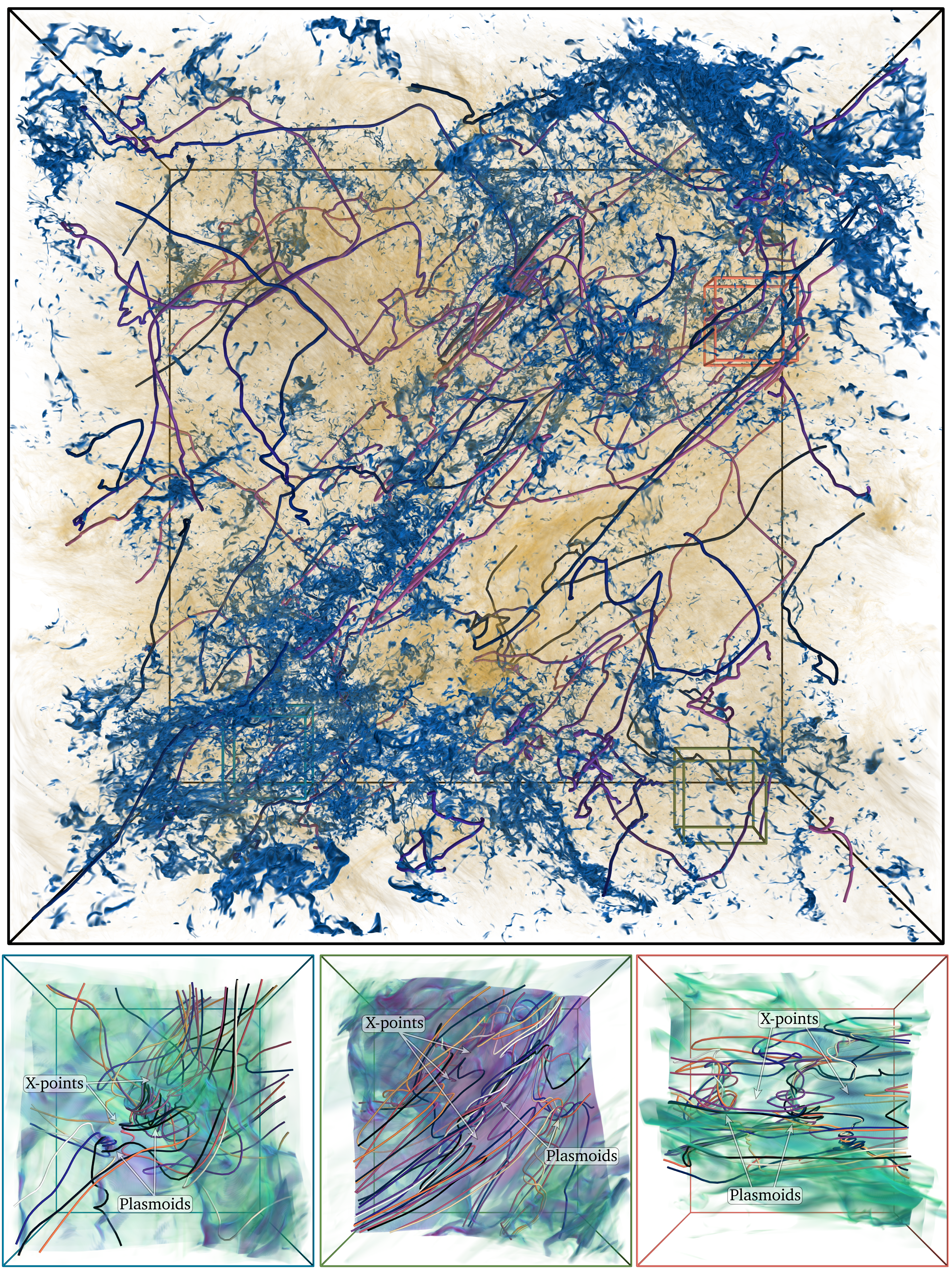
Figure 1: (Top) Volume rendering of the temperature (opaque blue corresponds to $T{\approx}T_{0}/100$, and transparent yellow corresponds to $T{\approx}10T_{0}$). Uniformly seeded magnetic field lines are shown in purple—many exhibiting helical patterns that trace plasmoids. (Bottom) Volume rendering of the electric current (increasing from transparent cyan to opaque magenta) and magnetic fields (randomly colored) in three sub-volumes containing plasmoids and “X-points” that are $L/8$ on a side. They are shown in full volume as colored cubes (left–blue, center–green, right–red) and respectively exemplify cold, asymmetric, and hot current sheets undergoing plasmoid mediated reconnection. A rotating movie of these can be found here.

In Fig. 1 and Fig. 2 we show 3D volume renderings and 2D slices of our fiducial simulation after 5 eddy turnover times of the warm gas ($5L/v_{\rm rms,warm}$). The top panels of both figures show the full volume, while the surrounding panels show zoom-ins on three regions. These regions (the same in both figures) exemplify the three distinct environments in which we find current sheets undergoing plasmoid-mediated magnetic reconnection: (i) within cold clumps, (ii) at the asymmetric interface of the cold and warm phases, and (iii) within the warm, volume-filling phase.

The volume on the whole is characterized by a bistable configuration with the vast majority of the gas residing near one of the two thermal equilibria. The cold gas morphology is clearly clumpy with structures on scales ranging from the nearly the size of the whole box ($\sim$10s pc) down to the grid scale (${\sim}10^{-2}$ pc). Many of these cold gas clumps show an elongated, filamentary structure with large aspect ratios (discussed in § 3.3).

The field lines shown in Fig. 1 give a sense for the large and small scale magnetic structure. While much of the volume is occupied by laminar fields, they also generically exhibit highly disturbed regions manifesting as small scale helical knots or “flux tubes”, which trace plasmoids and are hallmarks of tearing instability induced fast magnetic reconnection. This highlights that plasmoids form throughout the volume and can be found in the volume filling warm phase, the clumpy cold phase, and at the interface of the two. This is further supported by the 2D slice of the electric current, $\boldsymbol{j}\equiv\boldsymbol{\nabla}\times\boldsymbol{B}$, in the top left panel of Fig. 2. It is clear that there are numerous large current sheets with $L_{\rm CS}\gtrsim L/10$ throughout the volume—many of which are actively undergoing plasmoid-mediated magnetic reconnection. In Appendix A we show that similar large current sheets form in lower resolution simulations, but they are much more laminar and do not show signs of plasmoid instability.

The top panels of Fig. 1 and Fig. 2 further demonstrate that the thermodynamic and magnetic properties interact non-trivially. Regions with cold gas tend to be more magnetically dominated with $\beta<1$ (blue-green colors). This is likely due to magnetic field enhancement during cooling induced contraction. Moreover, the regions of highly disordered magnetic fields and large $\boldsymbol{j}$ tend to be associated with thermally unstable or cold gas.

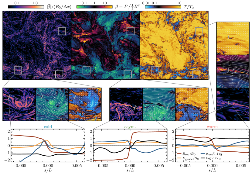
Figure 2: The top panels show 2D slices of the current density, plasma beta ($\beta$), and temperature. Zoom-ins on three regions with plasmoids are shown in the surround panels. In the zoom-in panels the in-plane magnetic fields are shown on top of the $\beta$ map, and the velocity vectors are shown on top of the temperature map. The three zoom in regions are the same as the sub-volumes shown in Fig. 1, and are in the same order. The zoom-ins are examples of the three different types of regions in which reconnection events that lead to plasmoid formation occur in our simulation: fully cold (left), interface of warm and cold (middle), fully warm (right). For each of the zoom-ins we show profiles perpendicular to the prominent current sheet of the magnetic field components perpendicular ($B_{\rm rec}$; this is the component that reconnects) and parallel ($B{}_{\rm g{\mskip-1.0mu}u{\mskip-1.0mu}i{\mskip-1.0mu}d{\mskip-1.0mu}e}$) to the local guide field, the velocity into the current sheet ($v{}_{\rm r{\mskip-1.0mu}e{\mskip-1.0mu}c}$; reconnection velocity) normalized by one tenth the local Alfvén velocity ($0.1v{}_{A}$), and the log of the temperature $\log_{10}(T/T_{0})$. The current sheets all show a change in direction of $B_{\rm rec}$, a reconnection speed of $v{}_{\rm r{\mskip-1.0mu}e{\mskip-1.0mu}c}\sim 0.01v{}_{A}$, and some compression of $B{}_{\rm g{\mskip-1.0mu}u{\mskip-1.0mu}i{\mskip-1.0mu}d{\mskip-1.0mu}e}$ in the cases that have any appreciable guide field. Animated version here.

Turning now to the zoom-in panels of Fig. 1 and Fig. 2 we get a better sense of the nature of reconnection in these environments and the morphology and properties of the plasmoids. Each region has one or more plasmoids and several clear X-points where the reconnection is actively occurring. Each of these regions exemplify the three distinct environments in which we find evidence for the plasmoid instability.

The zoom region shown on the left is an example of a current sheet that forms in the middle of a cold region. Current sheets like this arise in large part because of the compressive motions that result from the thermally unstable region rapidly contracting in on itself. The energy released during reconnection in these cold current sheets is quickly radiated away and the gas inside the plasmoid remains cold. This is demonstrated by temperature profile which remains cold along the ray passing through an X-point in the current sheet.

The zoom region shown in the middle is closely related to the first with the important distinction that the current sheet forms at the interface of the warm and cold phase. The pressure and magnetic field strength on either side of the current sheet is—in this example—nearly constant, thus the asymmetry is both in the temperature and density. Perpendicular to the current sheet the temperature changes by nearly a factor of 100 (lower middle panel of Fig. 2). These asymmetric current sheets are formed as a result of the flow of warm gas as it cools onto a cold clump with an oppositely oriented magnetic field. In the ISM, these strong cooling flows, which occur throughout the volume, can lead to the development of plasmoid unstable current sheets. Here reconnection may modify the phase balance as the heating is occurring directly in the thermally unstable phase where it can be most impactful. The plasmoids that form in these asymmetric current sheets tend to be highly elongated, often have cold interiors, and follow the surface of the larger cold clumps.

These first two cases are unique to the thermally unstable ISM-like environments we are considering and represent a new channel for magnetic reconnection. The reconnection is brought on by thermal instability induced tearing instabilities, and leads to the formations of, what we refer to as, cold plasmoids (i.e. plasmoids that form as result of radiative cooling and remain cold because of their short cooling times). As we discuss in § 4, cold plasmoids may be readily observable as Hi absorption and/or emission, and as sources for strong radio scattering. Furthermore, because of their magnetic insulation/shielding these cold plasmoids can survive for an appreciable fraction of the global dynamical time. In particular, their magnetic structure can make their lifetimes significantly longer than cold clumps of a similar size, which tend be mixed away on an eddy turnover time ($t_{\rm mix}\sim r_{\rm cl}/v_{\rm turb}(r_{\rm cl})\lesssim r_{\rm cl}/c_{\rm s,cold}\sim 0.1$ Myr for $r_{\rm cl}=0.1$ pc).

The cold and asymmetric plasmoid unstable current sheets can be contrasted to the final zoom region shown in right panels in which a current sheet forms in the volume filling warm phase as a result of the intermittency in the turbulent flow. The current sheet in this case has $\beta\gtrsim 100$, and the energy release from the reconnection has heated the immediate surrounding medium. This hot plasmoid formation, as we refer to it since it takes place in the hotter, volume-filling phase, has been seen in simulations of single phase highly magnetized turbulent environments (e.g. Chernoglazov et al., 2021; Galishnikova et al., 2022; Dong et al., 2022), and can be expected to be common throughout the volume filling region of the ISM.

Looking at the profiles along the rays that pass through the X-point of the most prominent current sheets in each of the zoom regions gives us a more detailed view into the properties of the current sheets. The temperature profiles clearly demonstrate our distinction between the cold, asymmetric, and warm current sheets. Each of the profiles exhibits a large reversal in the reconnecting component of the magnetic field ($B_{\rm rec}$) over a width of $\sim L/500$. The behavior of the component of the magnetic field aligned with the guide field ($B{}_{\rm g{\mskip-1.0mu}u{\mskip-1.0mu}i{\mskip-1.0mu}d{\mskip-1.0mu}e}$; i.e. the component aligned with the field direction in the middle of the current sheet) is noticeably different between the three profiles. Near the cold current sheet (left) $B{}_{\rm g{\mskip-1.0mu}u{\mskip-1.0mu}i{\mskip-1.0mu}d{\mskip-1.0mu}e}\sim B_{\rm rec}$, in the asymmetric current sheet $B{}_{\rm g{\mskip-1.0mu}u{\mskip-1.0mu}i{\mskip-1.0mu}d{\mskip-1.0mu}e}\lesssim B_{\rm rec}/4$ and remains coherent above and below the current sheet, and in warm current sheet $B{}_{\rm g{\mskip-1.0mu}u{\mskip-1.0mu}i{\mskip-1.0mu}d{\mskip-1.0mu}e}\sim 0$. Therefore, in addition to representing three different thermal properties these three current sheets also represent three guide field properties, namely strong, weak, and zero guide field, respectively.

Also shown in the profiles is the inflow velocity $v{}_{\rm r{\mskip-1.0mu}e{\mskip-1.0mu}c}$ (velocity toward the current sheet that is driving reconnection) normalized by one-tenth the average local Alfvén speed $0.1v{}_{A}$. In all cases $v{}_{\rm r{\mskip-1.0mu}e{\mskip-1.0mu}c}{\sim}0.01{-}0.03v{}_{A}$. This reconnection rate is comparable to the fast reconnection expected for tearing mediated reconnection (e.g. Loureiro et al., 2007; Bhattacharjee et al., 2009; Uzdensky et al., 2010).

3.2 Statistical Properties

We now shift our attention to the statistical properties of the simulation with an eye towards understanding the combined effects of turbulence, thermal instabilities, and magnetic reconnection.

3.2.1 Magneto-Thermal Phase Structure

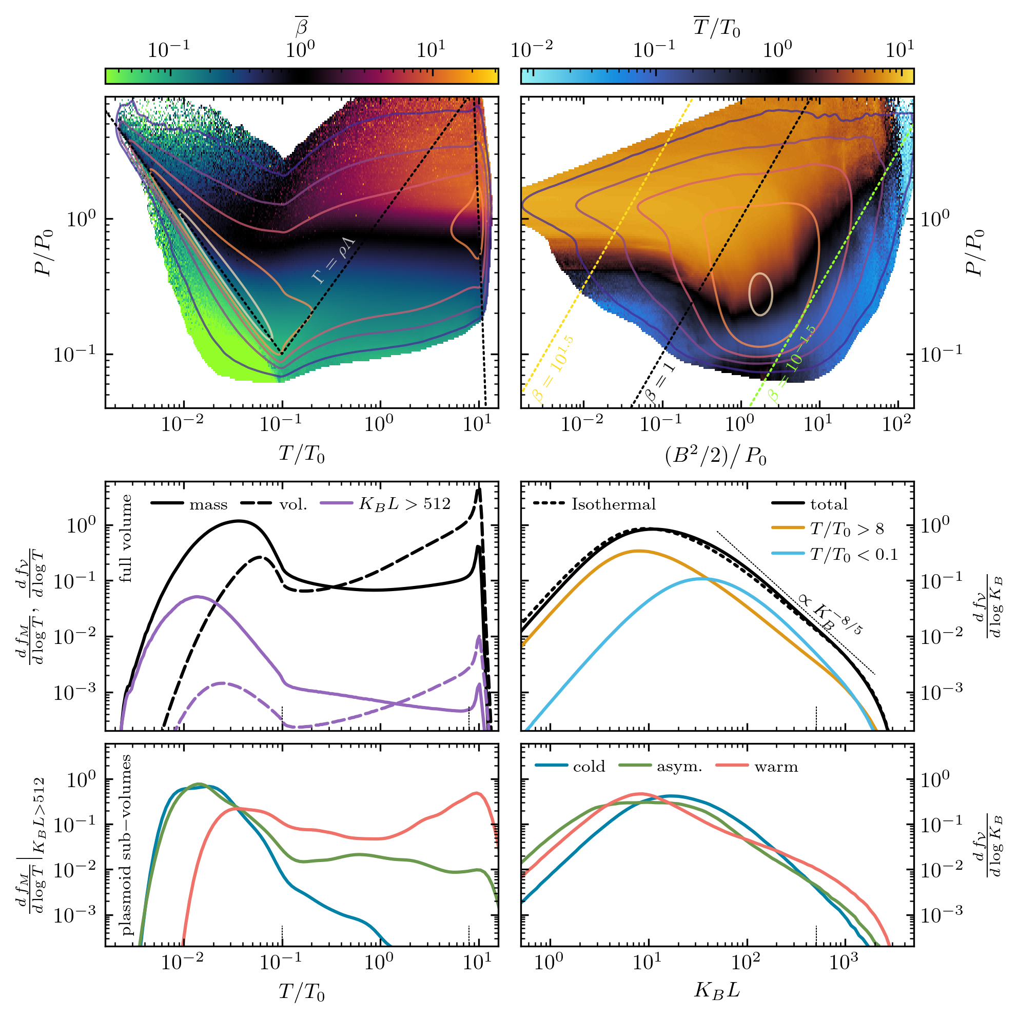
Figure 3: Summary of the magneto-thermal phase structure. The top left and right panels show the joint thermal pressure-temperature phase distribution colored by the average plasma beta ($\beta$), and thermal pressure-magnetic pressure phase distribution colored by the average temperature, respectively. The contours trace the fraction of the total mass per logarithmic bins spaced by 1 dex from $10^{-4}$ to 1 going from purple to white. The thermal equilibrium curve ($\Gamma=\rho\Lambda$) is shown in the black dotted line in the top left panel, and lines of constant $\beta$ are shown in the colored dotted lines in the top right panel. The mass ($f_{M}$; solid lines) and volume ($f_{\mathcal{V}}$; dashed lines) weighted temperature distributions are shown in the middle-left panel for the full volume (black lines) and for the high curvature regions only ($K_{B}>512/L$; purple lines). The mass weighted temperature distributions of the high curvature regions in the example plasmoid sub-volumes (same as in Fig. 1 and Fig. 2) are shown in the lower left panel. The volume distributions of magnetic curvature of the total volume (black), cold gas (blue), and warm gas (yellow) are shown in the middle-right panel. The dotted line shows the curvature distribution for the isothermal simulation. The curvature distributions in the plasmoid sub-volumes are shown in the lower right panel.

Fig. 3 provides an overview of the thermal and magnetic properties, and their correlations. We unpack these results incrementally starting with a discussion of the middle-left panel, which shows the temperature distribution of the mass (solid lines) and volume (dashed lines). The total mass of the domain is dominated by a broad distribution of cold gas with $T<T_{0}/10$. There is a peak of mass at the warm phase equilibrium near $10T_{0}$. Connecting these two peaks, and populating the thermally unstable regime, is a nearly flat distribution, that is continually depleted and repopulated by the combined effects of radiative cooling and heating, turbulent mixing, and reconnection heating. The volume, on the other hand, is dominated by the warm phase. This is a reflection of multiphase nature shown in the previous figures.

What determines the exact balance between the amount of mass in each of the two phases remains an open question. The answer depends on a non-trivial combination of the primary physical processes at play. The strength of conduction has been shown to regulate the balance in more simplified systems (e.g. Zel’Dovich & Pikel’Ner, 1969; Choi & Stone, 2012; Kim & Kim, 2013; Jennings & Li, 2021). Furthermore, we found in a simulation with a longer cooling time relative to the eddy turnover time (e.g., a smaller box), the fraction in the cold phase decreased. Likewise, increasing the strength of turbulence can significantly modify the phase distribution and in the extreme limits can erase the bimodal structure altogether (e.g. Vázquez-Semadeni et al., 2000; Gronke et al., 2022). How magnetic reconnection may impact this balance is an important future consideration given the difficulty of adequately resolving this process in ISM simulations.

To partially illuminate both the role of magnetic reconnection on the thermal structure and the role of thermal instabilities on the magnetic structure we also show with the purple lines in the middle-left panel of Fig. 3 the mass and volume temperature distributions of gas with large magnetic curvatures, $K_{B}~{}\equiv~{}(\hat{b}~{}\cdot~{}\boldsymbol{\nabla})~{}\hat{b}$, where $\hat{b}=\boldsymbol{B}/|\boldsymbol{B}|$. We adopt a threshold of $K_{B}>512/L$ which corresponds to the field changing direction in four cells or less (the center-right panel shows the full $K_{B}$ distribution and the small dashed line indicates our choice of threshold). High $K_{B}$ is good indicator of magnetic reconnection because of the large curvature inherent to plasmoids and X-points (as can be seen in the lower-right panel, which shows the curvature distribution of the plasmoid sub-volumes). The temperature distributions of the high $K_{B}$ gas are skewed toward more cold gas than the volume as a whole. This indicates that current sheet formation and reconnection is enhanced in the cold phase—likely as a result of the compression of the field due thermal instability induced contraction.

The curvature, $K_{B}$, alone is an imperfect tracer of plasmoids, so in the lower-left panel of Fig. 3 we show the temperature distribution of the high $K_{B}$ gas in the three example sub-volumes that contain clear plasmoids shown in the previous figures. All three sub-volumes exhibit a multiphase structure, however the cold current sheet has a negligible amount of warm, highly magnetically curved material. This demonstrates a key point that the heating by magnetic reconnection can be rapidly lost due to radiative cooling and is thus insufficient to drive the material to the hotter phase. How this heating impacts the global phase structure is an interesting discussion for future works.

The volume distribution of $K_{B}$ in the whole volume (black), cold gas (blue), warm gas (yellow), and in the example plasmoid sub-volumes is shown in the middle and lower right panels of Fig. 3. As expected the plasmoid sub-volumes have a large high curvature volume fraction owing to the fact that plasmoids are, by definition, comprised of highly curved field lines. At the high curvature end the total curvature distribution scales proportional to ${\propto}K_{B}^{-8/5}$. On average magnetic fields in cold gas ($T<T_{0}/10$) tend to be more curved than in the warm gas ($T>8T_{0}$), but the highest $K_{B}$ values are equally likely in either phase. The curvature distribution of all of the gas is remarkably similar to the isothermal driven turbulence simulation we ran for comparison.

To better understand the magneto-thermal phase distributions, in the the top left panel of Fig. 3, we show the joint distribution of pressure and temperature (contours trace the mass distribution and colors show the average $\beta$). As expected, the majority of the mass is found near the two stable thermal equilibria (i.e., along the negatively sloping portions of the equilibrium curve). The gas near the warm equilibrium is tightly clustered around $P\approx P_{0}$ and $T\approx 10T_{0}$, and has an average $\beta\sim 1$. The mass near the cold equilibrium is spread out along the stable equilibrium curve with $10^{-2.5}\lesssim T/T_{0}<0.1$ and $0.1\lesssim P/P_{0}<3$. The $\beta$ also varies in the cold phase, with the lower pressure cold gas having $\beta\lesssim 1/10$—indicating a strong compensation of the thermal pressure deficit by enhanced magnetic pressure ($B^{2}/2$). The enhancement of magnetic pressure in regions with lower thermal pressure means that, although the gas near the cold and warm thermal equilibria are not in thermal pressure equilibrium, they are close to being in total pressure equilibrium with $P+B^{2}/2\approx\text{constant}$. There is some mass with very low temperatures $T\lesssim T_{0}/100$ that has both high thermal pressure and low $\beta$, which is found in rapidly contracting thermally unstable regions that often host cold current sheets.

The upper right panel of Fig. 3 shows the joint mass distribution of thermal pressure and magnetic pressure and is colored by the average temperature in each bin. Most of the mass is found at a pressure of $P\approx 0.3P_{0}$ and a magnetic pressure of $B^{2}/2\approx 2P_{0}$, corresponding to $\beta\approx 10^{-0.75}$. The mass distribution has a distinct shape with a tail towards extremely low magnetic pressures. This tail follows a line of nearly constant total pressure. Gas moves both ways along lines of nearly constant total pressure. On the one hand, as warm gas cools and contracts it loses thermal pressure and gains a nearly equal proportion of magnetic pressure. On the other hand, highly magnetized gas that undergoes reconnection moves in the other direction in this phase space—the conversion of magnetic energy into thermal energy raises the thermal pressure of the gas as it loses magnetic pressure. In some cases, however, the magnetic reconnection heating is not sufficient to overcome the strong radiative cooling, so the end result is cold gas with low thermal pressure and low magnetic pressure, as can be seen by the lobe in the mass distribution of cold gas with $P\sim 0.3P_{0}$, and $B^{2}/2\lesssim 10^{-1}$. This is the case in the cold plasmoid formation channel exemplified by the cold and asymmetric current sheets shown in the previous two figures and in the bottom panels of Fig. 3. Note that in addition to heating, reconnection also accelerates gas, so some appreciable fraction of the magnetic energy is also being converted to small scale motions.

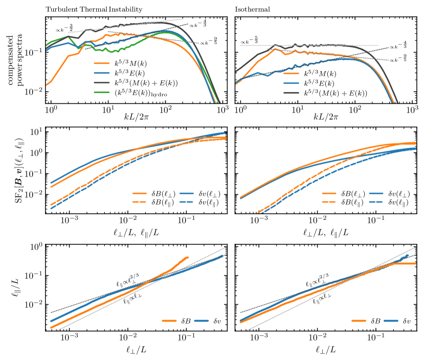
Figure 4: Statistical measures of the scale-dependent magnetic field and velocity structure. The left column shows the results from our turbulent thermal instability simulations and the right column shows the results from the isothermal turbulence simulation. The top panels show the magnetic $M(k)$ (orange) and velocity $E(k)$ (blue) power spectra, and their sum (black), compensated by $k^{5/3}$. Approximate power-law fits are shown in the thin dotted lines. Also shown in the upper left panel is the velocity spectrum from the non-magnetized simulation (green). The middle row shows the second order magnetic and velocity structure functions parallel and perpendicular to the local mean field. The bottom row shows the anisotropy of the magnetic and velocity fluctuations defined to be the scale at which the parallel and perpendicular structure function are equal.

The detailed analyses presented in Fig. 3 highlights the rich interplay between the thermodynamics, turbulence, and magnetic fields that combine to regulate the magneto-thermal phase structure of the ISM. While there is clearly still much to be understood (particularly in the computationally daunting limit of resolved explicit resistivity, conduction, and viscosity), we have shown that there are important correlated magnetic and thermal properties that when simulated at high enough resolution can lead to the formation of cold and hot plasmoids.

3.2.2 Scale Dependent Magnetic and Kinetic Structure

We now move on to an investigation of the structure of the magnetic and velocity fields as a function of scale, which is summarized in Fig. 4. The top row shows the magnetic ($M(k)\equiv\int d\Omega_{k}k^{2}\langle|\boldsymbol{B}(\boldsymbol{k})|^{2}\rangle/2$) and velocity ($E(k)\equiv\int d\Omega_{k}k^{2}\langle|\boldsymbol{v}(\boldsymbol{k})|^{2}\rangle/2$) power spectra compensated by $k^{5/3}$ for the turbulent thermal instability (left; $E(k)$ of a non-magnetized simulation shown in green) and isothermal driven turbulence simulations (right). On large scales (small $k$) in the turbulent thermal instability simulation $E(k)>M(k)$, but $M(k)$ is nearly flat while $E(k)\propto k^{-5/3}$, which leads to a reversal at intermediate scales ($4\lesssim kL/2\pi\lesssim 32$), in which $E(k)<M(k)$. Starting on intermediate scales there is a broad range of $k$ over which the $M(k)$ steepens to approximately follow $\propto k^{-9/5}$, and the $E(k)$ flattens to follow $\propto k^{-4/3}$. This transition and change in slopes occurs at $kL/2\pi\approx 12$. On small scales ($kL/2\pi\gtrsim 32$), $E(k)$ again dominates $M(k)$. Interestingly, despite the additional thermal physics included in this simulation the sum of the magnetic and velocity spectrum closely follows a scaling of $\propto k^{-3/2}$ over more than an order of magnitude in $k$, which is in line with standard MHD scaling predictions (e.g. Iroshnikov, 1964; Kraichnan, 1965). These general trends and slopes are well converged with numerical resolution down to 16 times lower resolution ($\Delta x=L/128$) than our fiducial simulation ($\Delta x=L/2048$; see Appendix A). Most of these same trends were found in the similar (albeit significantly lower resolution) turbulent thermally unstable MHD simulations presented by Kritsuk et al. (2017), with the notable exception of the dominance of $E(k)$ at large $k$, which we ascribe to slower cooling relative to turbulent mixing in their simulations.

In contrast, in the isothermal simulation the $M(k)>E(k)$ on all scales, although they do approach equipartition on the largest scales ($kL/2\pi\sim 1$) and on the smallest scales ($kL/2\pi\lesssim L/16\Delta x$). The total energy spectrum follows $\propto k^{-5/3}$ as predicted for anisotropic MHD turbulence (Goldreich & Sridhar, 1995, 1997). The velocity spectrum follows a shallower $\propto k^{-4/3}$ from $kL/2\pi\sim 1$ down to $\sim 100$, which is in agreement with other similar simulations (e.g. Grete et al., 2021). The magnetic spectrum, on the other hand, peaks around $kL/2\pi\sim 4$ and then follows a relatively steep $\propto k^{-9/5}$ slope down to the dissipative scale. These slopes, which are robust to changes in resolution, agree very well with the slopes of the thermally unstable simulations at $kL/2\pi\gtrsim 12$.

Comparing the spectra of the thermally unstable and isothermal simulations highlights the enhanced kinetic energy at small scales in the thermally unstable simulations. This cannot be due to magnetic reconnection alone since both exhibit plasmoid-mediated magnetic reconnection. Furthermore, with our resolution, $\Delta x=L/2048$, only the largest current sheets are resolved and the scales on which plasmoids are forming are somewhat impacted by numerical dissipation. We, therefore, cannot say that at yet higher resolution that plasmoid-mediated magnetic reconnection would or would not change the power spectra as is predicted for a turbulence with a strong mean field (Boldyrev & Loureiro, 2017; Dong et al., 2022). Comparing to the spectrum of a non-magnetized turbulent thermally unstable simulation, which also exhibits a similar large $k$ peak in $E(k)$ (green line in top left panel of Fig. 4), supports the notion that strong radiative cooling is driving small scale motions in the thermally unstable simulations. Further evidence supporting this picture comes from the fact that as we reduced the strength of cooling in our simulations (not shown) the magnitude of the small scale (large $k$) peak in the velocity spectra also decreased. The spectra in both the magnetized and non-magnetized turbulent thermally unstable simulations change slopes at $k\sim 10-20$, which is a reflection of the imprint of cooling on the flows.

The energy spectra are inherently isotropic and so cannot provide any information on the degree to which velocity and magnetic field perturbations are aligned with the local mean magnetic field. Thus to further understand the structure of the magnetic and turbulent velocity fields, we turn to the structure functions shown in the second row of Fig. 4. They encode the scale-dependent structure and anisotropy with respect to the local magnetic-field direction. We adopt the two-point second order structure function that is defined for the magnetic field to be ${\rm SF}_{2}[\boldsymbol{B}](\boldsymbol{\ell})\equiv\langle|\boldsymbol{B}(\boldsymbol{x})-\boldsymbol{B}(\boldsymbol{x}+\boldsymbol{\ell})|^{2}\rangle$, and equivalently for the velocity field. In a sufficiently magnetized plasma these structure functions can show a dependence on the degree of alignment between the separation vector $\ell$, and the local mean magnetic field, which we define to be $\overline{\boldsymbol{B}}_{\ell}\equiv(\boldsymbol{B}(\boldsymbol{x})+\boldsymbol{B}(\boldsymbol{x}+\boldsymbol{\ell}))/2$. We, therefore, consider the parallel and perpendicular structure functions, which are defined to be ${\rm SF}_{2}[\boldsymbol{B}](\ell_{\parallel})\equiv\langle|\boldsymbol{B}(\boldsymbol{x}){-}\boldsymbol{B}(\boldsymbol{x}{+}\boldsymbol{\ell})|^{2};0{\leq}\theta_{\ell}{<}\tfrac{\pi}{36}\rangle$, and ${\rm SF}_{2}[\boldsymbol{B}](\ell_{\perp})\equiv\langle|\boldsymbol{B}(\boldsymbol{x}){-}\boldsymbol{B}(\boldsymbol{x}{+}\boldsymbol{\ell})|^{2};\tfrac{17\pi}{36}{\leq}\theta_{\ell}{<}\tfrac{\pi}{2}\rangle$ where $\theta_{\ell}\equiv\arccos|\overline{\boldsymbol{B}}_{\ell}{\cdot}\boldsymbol{\ell}/\overline{B}_{\ell}\ell|$ is the angle between the displacement vector and the mean magnetic field direction (cf. St-Onge et al., 2020). The average difference in magnetic field and velocity at a given distance perpendicular to the local mean magnetic field is significantly larger than the difference the same distance parallel to the local mean magnetic field in both the thermally unstable and isothermal simulations. This is inline with the notion that it is easier to perturb the field and the flow along the field lines than it is perpendicular to them.

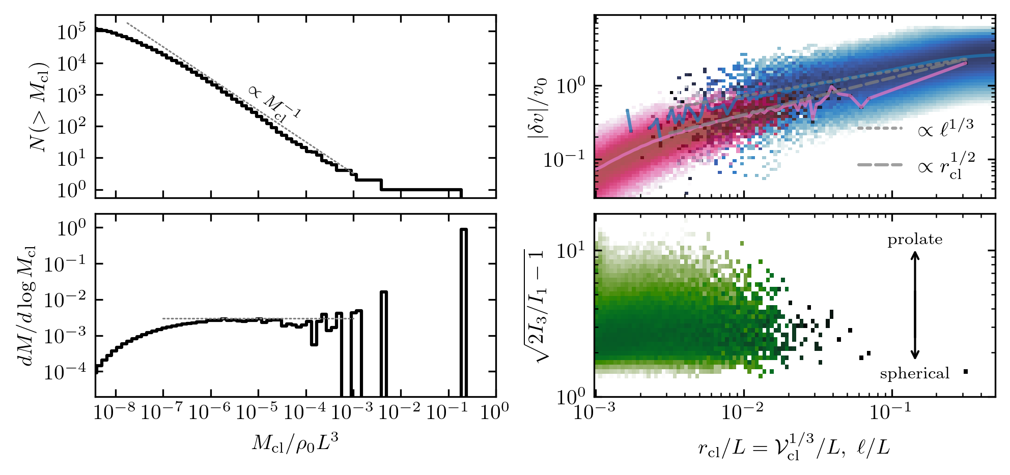
Figure 5: Distribution and properties of the cold clumps in our fiducial turbulent thermally unstable simulation. Clumps are defined to be contiguous regions of material on the cold stable thermal equilibrium. The left panels show the distribution of clump masses. The upper right panel shows the internal velocity dispersion as a function of clump size (given by the cube root of the clump volume $r_{\rm cl}=\mathcal{V}_{\rm cl}$) in pink, and the pairwise velocity difference of the clumps as a function of separation ($\ell$) in blue. The solid lines show the median values. The lower right panel shows the clump elongation versus clump size with larger values indicating highly elongated clumps, and values $\sim 1-2$ indicating nearly spherical objects.

We can take this one step farther by investigating the scale dependent anisotropy of both the magnetic field and velocity fluctuations, which are shown in the bottom row of Fig. 4. This is calculated by equating the parallel and perpendicular structure functions, which yields the parallel length scale $\ell_{\parallel}$ as a function of the perpendicular length scale $\ell_{\perp}$ (or vice versa) for both the magnetic fields ($\ell_{\parallel,\delta B}$) and the velocity ($\ell_{\parallel,\delta v}$) fluctuations (e.g. Cho & Vishniac, 2000; Maron & Goldreich, 2001). In the isothermal simulation when $\ell_{\perp}\gtrsim 8\Delta x$ the magnetic field and velocity fluctuations are increasingly elongated along the local mean magnetic field with decreasing scale following the predicted $\ell_{\parallel}\propto\ell_{\perp}^{2/3}$ (Goldreich & Sridhar, 1995). On the other hand, in the thermally unstable simulation only the velocity fluctuations follow this scaling, while the magnetic fluctuations instead have $\ell_{\parallel,\delta B}$ scaling linearly or even super-linearly with $\ell_{\perp,\delta B}$. This change in the anisotropy scaling must come about due to the cooling inducing flows that are sufficiently strong to rearrange the field.

3.3 Clump Mass Distributions

We end this section with a brief look at the properties of the cold clumps that form in our fiducial turbulent thermally unstable simulation. We identify cold clumps in the simulation using a pressure-temperature cut that selects gas that is close to the cold thermal equilibrium (see top left panel of Fig. 3). The top left panel of Fig. 5 shows clump mass, $M_{\rm cl}$, distribution, and the bottom left panel shows the amount of mass contained in cold clumps per logarithmic bin in clump mass. Over nearly 4 orders of magnitude in clump masses the distribution closely follows a Zipf’s Law like distribution with an index of -1, which has commonly been observed in other turbulent multiphase systems (see Gronke et al., 2022, for a recent investigation of the origin of this distribution). This distribution yields nearly equal mass per logarithmic bin in clump mass. In terms of total mass, however, the distribution is dominated by a single large clump that contains $>30$ percent of all the mass in the domain. The amount of mass contained in this single large cloud is dependent on the strength of cooling. In similar simulations with weaker cooling relative to turbulent mixing, the amount of mass in the largest cloud is reduced dramatically, while the slope of the main distribution is nearly unchanged.

In the top right panel of Fig. 5 we show the intra- and inter-clump velocity distributions as a function of clump size and separation, respectively. The intra-clump velocity (defined internal velocity standard deviation $v_{\rm cl,std}$) versus clump size distribution is shown in the pink along with the median relation. The distribution closely follows a Larson’s Law like scaling with $v_{\rm cl,std}\propto r_{\rm cl}^{1/2}$ (Larson, 1981). This is also consistent with the scaling for supersonic Burgers turbulence, as expected since $v_{\rm cl,std}>c_{\rm s,cl}\approx 0.1v_{0}$ for all clumps. The inter-clump velocity (difference between two clumps; the mean of which is the first order clump velocity structure function) follows a somewhat flatter relation with $\langle|\delta v_{\rm cl}(\ell)|\rangle\propto\ell^{1/3}$, which follows the prediction for Kolmogorov-like turbulence and is consistent with recent observations (Ha et al., 2022). The difference between these two scalings points to the cold clouds being entrained in a background sub/trans-sonic turbulent flow while having supersonic internal motions.

In the bottom right panel Fig. 5 we show the elongation distribution as a function of clump size. To quantify the elongation we adopt $(2I_{3}/I_{1}-1)^{1/2}$ as a metric where $I_{3}$ and $I_{1}$ are the largest and smallest moments of inertia of the clump, which for a prolate (cigar shaped) ellipsoid equals the ratio of the length of the longest axis to the shortest. For a sphere this takes a value of 1, and for an thin disk this reaches $5^{1/2}$. Although this quantity is imperfect for distinguishing between marginal cases it clearly demonstrates that the cold clumps in our simulation tend to be highly elongated structures.

4 Discussion and Conclusion

4.1 Summary

We present the highest resolution (to our knowledge) magnetohydrodynamic simulation of a thermally unstable turbulent medium to date. We show that large current sheets unstable to plasmoid-mediated reconnection form regularly throughout the volume. The current sheets that reconnect and give rise to plasmoids that develop in three distinct environments: within the coldest phase, at the asymmetric interface of the cold and warm phases, and within the volume-filling warm phase. We show the rich magneto-thermal phase structure that develops, in which that most of the mass is in the highly magnetized cold phase, and that the regions of highest magnetic curvature span a broad range in temperatures. Furthermore, we show that thermal instabilities and magnetic fields change the scale dependent magnetic and velocity structure. This is achieved by comparing our fiducial simulation to an isothermal simulation and a simulation without magnetic fields. The comparison highlights that the total energy spectrum is flatter in the thermally unstable case, and that the velocity spectrum dominates on both large and small scales with cooling likely being responsible for the increase in small scale kinetic energy. Additionally, in the isothermal simulation both the magnetic and velocity perturbations follow the predicted increase in anisotropy relative to the local mean magnetic field with decreasing scale. In the thermally unstable simulation, however, only the velocity perturbations follow this scaling whereas the magnetic perturbations are more isotropic and maintain the same small degree of anisotropy on all scales. Lastly, we show that the clumps of cold gas in the thermally unstable simulation mostly follow a scale free mass distribution with equal mass per logarithmic bin in clump mass, with the exception of the largest clump that contains most of the mass in the entire simulation. These clumps tend to be highly elongated and exhibit a size versus internal velocity relation consistent with supersonic turbulence, and a relative clump distance-velocity scaling consistent with subsonic motion.

4.2 Known Limitations

While our simulations presents a major step forward in resolving the small scale magneto-thermal properties of the ISM they are clearly, and intentionally, highly idealized, which means there are important caveats that should be taken into account. Although our piecewise power law cooling and heating source terms capture the important general trends applicable to a range of systems, they miss important subtleties essential for detailed comparison to specific systems. Likewise our simulations do not track changes the chemistry and ionization state of the system, which can have important observational and physical impacts. For our 3D simulations, we rely on numerical dissipation to break the magnetic flux freezing when in reality explicit non-ideal MHD effects, such as ohmic dissipation, should be mediating the reconnection. Resolving these effects in the plasmoid-mediated regime in 3D is extremely computationally expensive and has only been achieved once in a single phase, decaying turbulence simulation (Dong et al., 2022). We stress, however, that in Appendix B we use 2.5D simulations to test the impact of using resolved explicit dissipation and find strong indications to believe that the physical processes we see are robust. Similarly, we do not include explicit conduction and viscosity in our 3D simulations which is expected to be relevant (e.g. Cowie & McKee, 1977) and highly anisotropic (e.g. Choi & Stone, 2012), and may alter the phase structure and flows in important ways. Supernovae, which we have not included in our simulations, generate a third, hottest phase (McKee & Ostriker, 1977) and drive more compressive turbulence than what we assumed. It remains to be seen how reconnection proceeds in the hot phase, which will be much more subsonic, and in the presence of more compressive flows. And finally, our simulations do not include the impact of gravity, which may modify the dynamics particularly in the densest regions and may lead to the development of converging flows that can form current sheets. Despite these caveats our findings are relevant to many outstanding ISM observation puzzles and may provide a useful guide to better understanding the physical processes at play in the ISM.

4.3 Observational Implications

In the interstellar medium it is well known that structures exist across a vast range of scales spanning more than 10 orders of magnitude from hundreds of pc down to hundreds of km (Armstrong et al., 1995). On the few to ${\sim}10^{4}$ AU scale there is ample observational evidence for tiny scale atomic and ionized structures (TSAS and TSIS, respectively) that probe the poorly understood dissipation processes (for a useful overview, see Stanimirović & Zweibel, 2018). These structures manifest as extremely small or fast spatial or temporal variations in Hi absorption (TSAS) and as extreme scattering events and interstellar scintillation in radio observations of both quasars and pulsars (TSIS). Observational models favor either very high density spherical structures or highly elongated structures viewed lengthwise. The plasmoids in our simulation are both dense and elongated, and they are found on the smallest scales we are able to probe which is comparable to the larger end of the observed sizes ($\Delta x\sim 5\times 10^{3}$ AU). Plasmoids will only become more common at smaller scales if we were able to probe higher resolutions. The thermal instability induced cold plasmoids are thus good candidates for TSAS, and the hot plasmoids are good candidates for TSIS. A careful comparison will need to be made to show this connection more concretely, but the qualitative agreement is compelling. Furthermore, the magnetic topology of the plasmoids provides a natural confinement and insulation which will tend to extend the lifetime of these small structures. Our scale separation between the outer and dissipative scales is, however, limited, so a better understanding of how these results scale is needed.

On somewhat larger scales recent work has uncovered highly elongated thin Hi structures referred to as Hi fibers (Clark et al., 2014). These fibers are dense ($n\sim 14\,{\rm cm}^{-3}$), have lengths on the order of a few pc and widths $\lesssim 0.1$ pc (possibly $\ll 0.1$ pc since the widths are unresolved in current observations). The properties of the cold plasmoids in our simulations are highly reminiscent of the properties of the Hi fibers and may provide a physical explanation for their origin. This supports a physical picture in which TSAS and Hi fibers are cold plasmoids seen either length-wise or edge-wise. A detailed look (which we defer to a future work) at the properties of the cold clumps in our simulations, and in particular how aligned they are with the local magnetic field may help shed light on the nature of ISM turbulence (e.g. González-Casanova & Lazarian, 2017) and far ranging observations such as foregrounds in the Cosmic Microwave Background (Clark et al., 2021).

4.4 Physical Implications

Our findings have potentially major implications for the transport of cosmic rays (CRs) in the ISM. CRs play an essential role in the evolution of galaxies (Zweibel, 2017), but their impact depends strongly on their transport (Salem & Bryan, 2014; Ruszkowski et al., 2017; Hopkins et al., 2020; Quataert et al., 2022a, b). CR transport is regulated by the scattering with small-scale electromagnetic fluctuations that are either self-excited (Kulsrud & Pearce, 1969; Skilling, 1971) or preexist in the ambient turbulent medium (e.g. Chandran, 2000; Yan & Lazarian, 2004). Recent work has shown that both of these models make predictions that are in significant tension with existing observations (Kempski & Quataert, 2022; Hopkins et al., 2021). Two aspects of our simulations represent attractive solutions to the shortcomings of the model in which CRs scatter as a result of turbulence in the ambient medium. First, the magnetic fluctuations in our thermal instability simulation do not exhibit an increase in anisotropy with decreasing scale (Fig. 4). This is crucial because anisotropic eddies are very inefficient at scattering CRs (Chandran, 2000). Second, plasmoids are regions of extremely high magnetic curvature, so a CR confined to move along a field line that encounters a plasmoid may efficiently scatter if its Larmor radius is comparable to the curvature radius, thus making plasmoids an attractive means to scatter CRs as suggested by Kempski & Quataert (2022). Furthermore, the size spectrum of plasmoids may naturally lead to an energy dependent CR diffusion coefficient inline with what is needed to reproduce Milky Way observations (Amato & Blasi, 2018). We plan to investigate CR scattering in plasmoid dominated MHD turbulence in a future work.

An additional implication of our ISM plasmoid findings is that the lifetime of the smallest structures may be significantly enhanced. The highly anisotropic nature of thermal conduction in the ISM (e.g. Spitzer, 1962) means that conductive evaporation will be reduced since the interior of a plasmoid will be well insulated due to the fact that, as can be clearly seen in Fig. 1, it is almost entirely magnetically disconnected from the surrounding medium. We, therefore, expect to find clumps on scales smaller than the standard isotropic Field length (Begelman & McKee, 1990). This is supported by the findings of thermal instability simulations with anisotropic thermal conduction (Sharma et al., 2010; Choi & Stone, 2012; Jennings & Li, 2021). Furthermore, the enshrouding magnetic fields will also limit hydrodynamic mixing of the plasmoid with the surroundings (Chandrasekhar, 1961), thereby extending the lifetime and minimum size that should be expected.

4.5 Outlook

This work represents the beginning of a new line of inquiry into the nature of the magnetized multiphase ISM. There remains much to be done to strengthen and extend our initial findings, and to connect them to observations and other physical processes. We have clearly demonstrated that the plasmoid instability and the associated fast magnetic reconnection is a common occurrence in the interstellar medium and can be induced by thermal instabilities. Furthermore, given the simplicity of our approach our findings are likely to apply to a broad range of systems beyond the ISM, such as the circumgalactic medium, the intracluster medium, and stellar coronae.

Appendix A Convergence in 3D

Although on the smallest scales we do not expect our results to be converged since we do not include explicit resolved dissipation processes, on large scales our findings are quite well converged. We demonstrate this by looking at the convergence of the velocity and magnetic field power spectra in Fig. 6 in which we compare our fiducial turbulent thermally unstable MHD simulation to simulations with up to 16 times lower resolution. The velocity power spectrum, $E(k)$, and magnetic field power spectrum, $M(k)$, on the largest scales are very well converged. At intermediate scales, $4\lesssim kL/2\pi\lesssim 100$, the slope and normalization of $E(k)$ is robust to changes in resolution particularly above $L/\Delta x\geq 512$. $M(k)$ on these same intermediate scales is somewhat less well converged indicating that the increased numerical resistivity at lower resolutions may impact the resolved scales, and that we may be below/just at the critical threshold to form plasmoids in this case. The sum of the velocity and magnetic field spectra is remarkably well converged.

In the top panel of Fig. 7 we show that the bulk temperature distribution is extremely well converged with almost no appreciable difference across the full range of resolutions we explored. The bottom panel, on the other hand, shows the curvature distribution, which, not surprisingly, is less well converged with lower resolution simulations tending to have lower curvature on average and less very curved fields. The slope of the curvature distribution, however, is unchanged in simulations with differing resolutions.

Lastly, in Fig. 8 we give a qualitative picture of the importance of resolution, by showing 2D slices of current, and temperature in simulations with $\Delta x/L=1/128$ to $1/2048$. In all simulations it is clear that large exist but going from low to high resolution the current sheets become far more disturbed and much less laminar. The low resolution simulations show no signs of the plasmoid instability. This highlights the essential need for very high resolution to properly capture the onset of plasmoid formation. We find that our fiducial resolution of $\Delta x/L=1/2048$ is just barely sufficient. The temperature field structure also changes dramatically with resolution with far more small clumps in the higher resolution simulations.

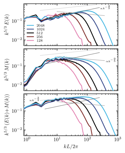
Figure 6: Comparison of the velocity, magnetic, and total energy spectra for turbulent thermally instability simulations with resolutions ranging from $L/\Delta x=2048$ to 128. The approximate power-law fits to the highest resolution simulation are repeated in each panel to ease comparison.

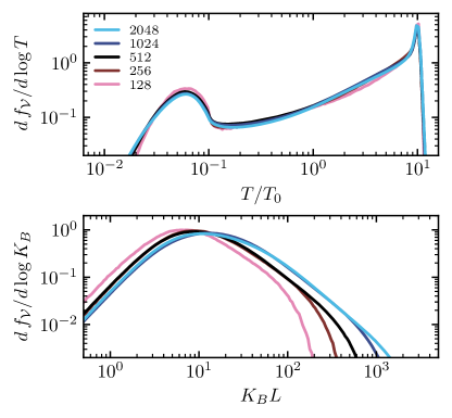
Figure 7: Comparison of the temperature and curvature distributions for turbulent thermally instability simulations with resolutions ranging from $L/\Delta x=2048$ to 128.

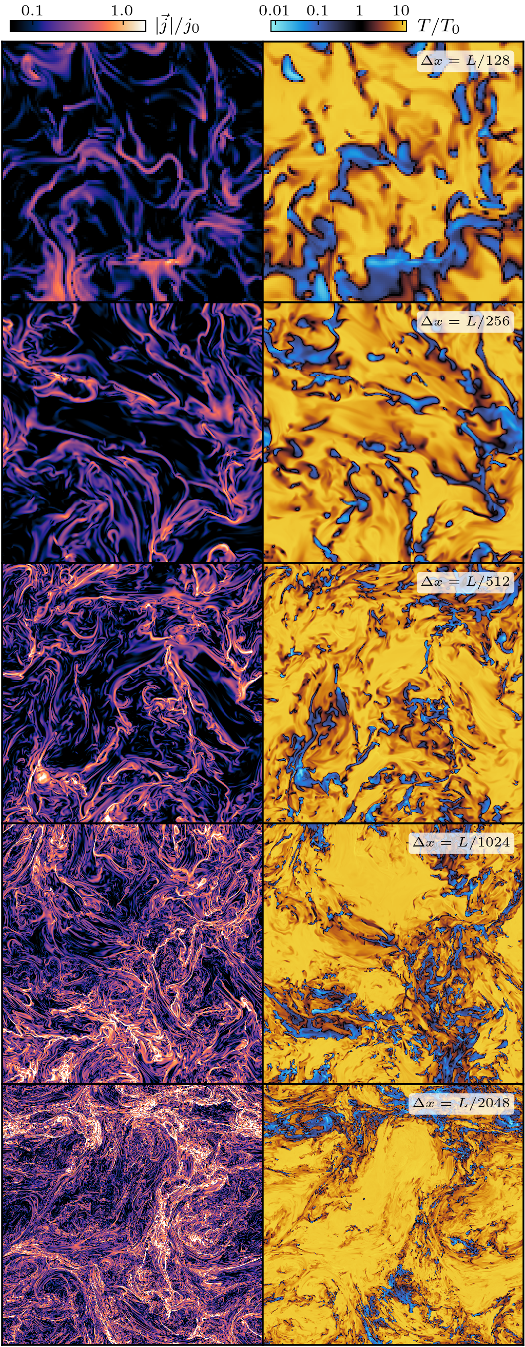
Figure 8: 2D slices of current and temperature from simulations with the same parameters as our fiducial simulation but with lower resolution ranging from $\Delta x/L=1/128$ to 1/2048. The current is normalized by $j_{0}=B_{0}/512$. A multiphase medium clearly develops, as do large current sheets, however the current sheets in simulations with worse resolution do not show as clear signs of the plasmoid instability because the large numerical dissipation.

Appendix B Fully Resolved 2.5D Simulations

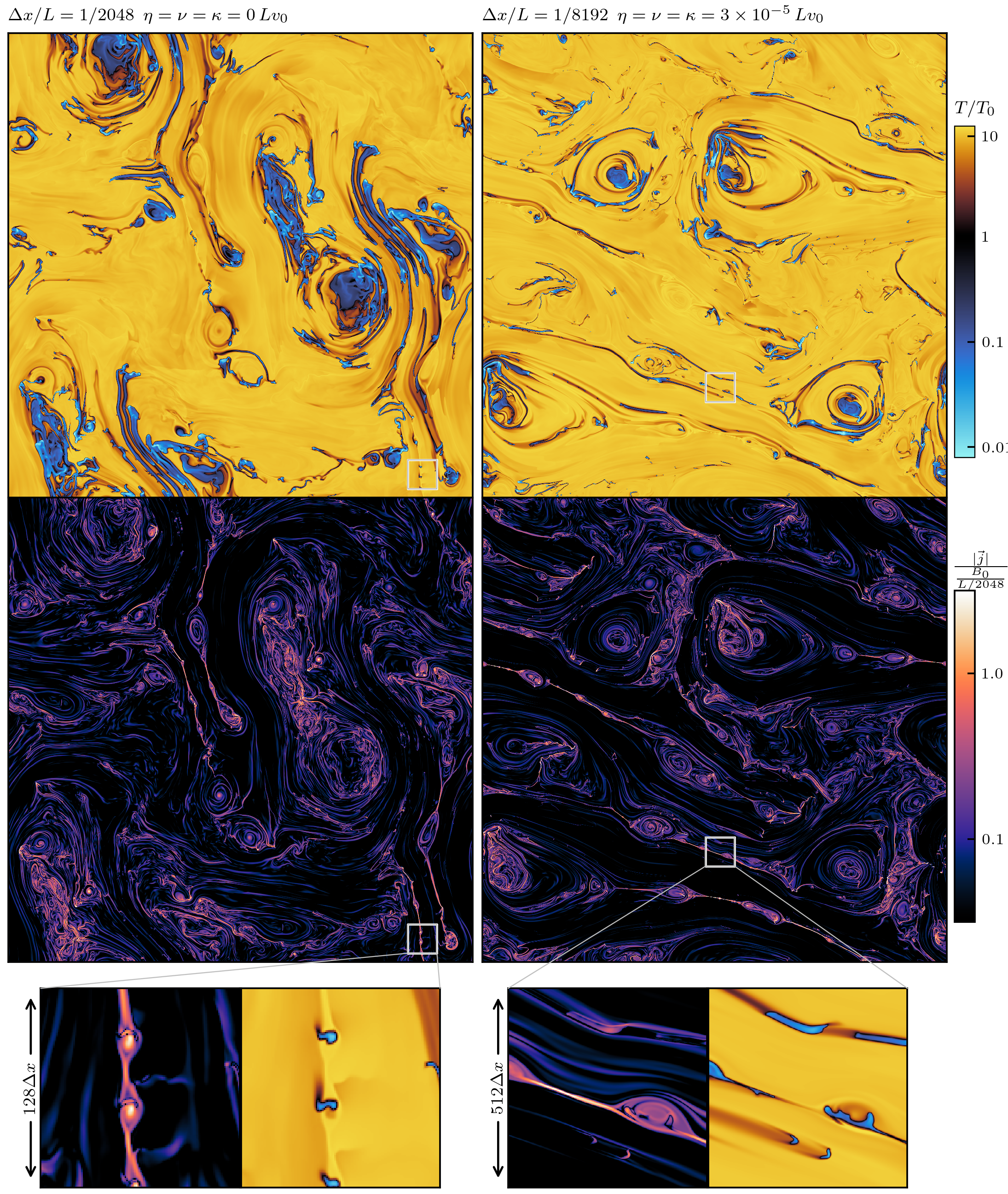
Figure 9: Comparison of the temperature (top) and current (bottom) in 2D simulations with either no explicit dissipation processes and a resolution of $\Delta x/L=1/2048$ (left), or with small but fully resolved dissipation processes and a resolution of $\Delta x/L=1/8192$ (right). Also show are zoom-ins onto regions 1/16th of the domain centered on tearing unstable current sheets forming cold plasmoids. On both large and small scales there is a marked similarity between these two simulations indicating that numerical dissipation in simulations with high enough resolution can enable plasmoid mediated reconnection in a manner qualitatively consistent with resolved simulations with explicit dissipation.

Simulations with non-zero explicit resistivity that are high enough resolution to resolve plasmoid unstable current sheets are extremely expensive in 3D. As a result, throughout this work we have relied on numerical resistivity. This implicitly assumes that the nature of numerical dissipation is sufficiently similar to explicit resistivity that the plasmoid instability is not changed in important ways. To assess the validity of this simulation we compare a pair of 2.5D simulations with the same conditions as our fiducial simulation. In one of the simulations we adopt the same spatial resolution ($\Delta x/L=1/2048$) and no explicit dissipation processes, and in the other we adopt 4 times higher resolution ($\Delta x/L=1/8192$) and explicit resistivity, conductivity, and viscosity ($\eta=\kappa=\nu=3\times 10^{-5}Lv_{0}$). This corresponds to Reynolds number of $Re=3\times 10^{4}$, a Prandtl number of $Pr=1$, and a magnetic Prandtl number of $Pr_{M}=1$. At this resolution the dissipation scales are well resolved and sufficiently small to not hinder the onset of the plasmoid instability.

In Fig. 9 we compare the temperature and current of the two 2.5D simulations. Due to the different nature of turbulence in 2.5D compared to 3D we make this comparison after one eddy turn over time, which is sufficient for the development of fluctuations on all scales and the formation of large current sheets. On a qualitative level it is clear that the thermal and magnetic properties on both large and small scales are very similar. We include zoom-ins on current sheets that are in the process of reconnecting and forming cold plasmoids. These highlight that although the X-points in the lower resolution simulation without explicit dissipation are resolved by only $\sim 4$ cells while in the higher resolution simulation with explicit dissipation they are resolved by $\gtrsim 10$ cells the overall dynamics and the resulting plasmoids are very similar.

Appendix C Cooling and Heating Source Terms

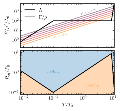
Figure 10: (Top) The black line shows the cooling function, and the colored lines show the heating function for a range of pressures. (Bottom) The equilibrium pressure for these cooling and heating functions versus temperature.

The exact functional form of the cooling curve we adopt is given by

$$\Lambda=\xi\Lambda_{0}{\times}\begin{cases}(T/T_{\rm lo})^{\alpha_{\rm lo}}&T_{\rm lo}<T\\ 1&T_{\rm lo}\leq T\leq T_{\rm hi}\\ (T/T_{\rm hi})^{\alpha_{\rm hi}}&T_{\rm hi}<T\end{cases}$$ (C1)

where $\xi$ is a dimensionless parameter that controls the strength of cooling, $T_{\rm lo}=T_{\rm cold}^{1-1/\alpha_{\rm lo}}$, and $T_{\rm hi}=T_{\rm warm}^{1-1/\alpha_{\rm hi}}$. We adopt $\alpha_{\rm lo}=2$ and $\alpha_{\rm hi}=20$ to roughly match a Milky Way ISM like cooling curve, and take $T_{\rm cold}=T_{0}/100$, and $T_{\rm warm}=10T_{0}$, which in Milky Way like conditions correspond to roughly 10 K and $10^{4}$ K, respectively.

We use a constant heating rate $\Gamma=(P_{0}/k_{B}T_{0})\xi\Lambda_{0}$, which guarantees that $T_{\rm cold}$ and $T_{\rm warm}$ are stable equilibria when $P=P_{0}$. In our primary simulations we adopt $\xi=100$, although we also performed several simulations with $\xi=1$ and 10. This parameter $\xi$ can be thought of as a proxy for the ratio of the eddy turnover timescale to the thermal instability timescale, thus our choice of $\xi\gg 1$ indicates we are in the rapidly thermally unstable regime and can expect there to be a bistable equilibrium phase structure.

The top panel of Fig. 10 shows the cooling and heating rates as a function of temperature. The bottom panel shows the equilibrium pressure as a function of temperature.

References

- Amato & Blasi (2018) Amato, E., & Blasi, P. 2018, Advances in Space Research, 62, 2731, doi: 10.1016/j.asr.2017.04.019
- Armstrong et al. (1995) Armstrong, J. W., Rickett, B. J., & Spangler, S. R. 1995, ApJ, 443, 209, doi: 10.1086/175515
- Begelman & McKee (1990) Begelman, M. C., & McKee, C. F. 1990, ApJ, 358, 375, doi: 10.1086/168994
- Bhattacharjee et al. (2009) Bhattacharjee, A., Huang, Y.-M., Yang, H., & Rogers, B. 2009, Physics of Plasmas, 16, 112102, doi: 10.1063/1.3264103
- Boldyrev & Loureiro (2017) Boldyrev, S., & Loureiro, N. F. 2017, ApJ, 844, 125, doi: 10.3847/1538-4357/aa7d02
- Burkhart et al. (2009) Burkhart, B., Falceta-Gonçalves, D., Kowal, G., & Lazarian, A. 2009, ApJ, 693, 250, doi: 10.1088/0004-637X/693/1/250
- Chandran (2000) Chandran, B. D. G. 2000, ApJ, 529, 513, doi: 10.1086/308232
- Chandrasekhar (1961) Chandrasekhar, S. 1961, Hydrodynamic and hydromagnetic stability
- Chernoglazov et al. (2021) Chernoglazov, A., Ripperda, B., & Philippov, A. 2021, ApJ, 923, L13, doi: 10.3847/2041-8213/ac3afa
- Cho & Vishniac (2000) Cho, J., & Vishniac, E. T. 2000, ApJ, 539, 273, doi: 10.1086/309213
- Choi & Stone (2012) Choi, E., & Stone, J. M. 2012, ApJ, 747, 86, doi: 10.1088/0004-637X/747/2/86
- Clark et al. (2021) Clark, S. E., Kim, C.-G., Hill, J. C., & Hensley, B. S. 2021, ApJ, 919, 53, doi: 10.3847/1538-4357/ac0e35
- Clark et al. (2014) Clark, S. E., Peek, J. E. G., & Putman, M. E. 2014, ApJ, 789, 82, doi: 10.1088/0004-637X/789/1/82
- Cowie & McKee (1977) Cowie, L. L., & McKee, C. F. 1977, ApJ, 211, 135, doi: 10.1086/154911
- Dong et al. (2018) Dong, C., Wang, L., Huang, Y.-M., Comisso, L., & Bhattacharjee, A. 2018, Phys. Rev. Lett., 121, 165101, doi: 10.1103/PhysRevLett.121.165101
- Dong et al. (2022) Dong, C., Wang, L., Huang, Y.-M., et al. 2022, arXiv e-prints, arXiv:2210.10736. https://arxiv.org/abs/2210.10736
- Elmegreen & Scalo (2004) Elmegreen, B. G., & Scalo, J. 2004, ARA&A, 42, 211, doi: 10.1146/annurev.astro.41.011802.094859
- Falgarone et al. (2008) Falgarone, E., Troland, T. H., Crutcher, R. M., & Paubert, G. 2008, A&A, 487, 247, doi: 10.1051/0004-6361:200809577
- Field et al. (1969) Field, G. B., Goldsmith, D. W., & Habing, H. J. 1969, ApJ, 155, L149, doi: 10.1086/180324
- Furth et al. (1963) Furth, H. P., Killeen, J., & Rosenbluth, M. N. 1963, Physics of Fluids, 6, 459, doi: 10.1063/1.1706761
- Galishnikova et al. (2022) Galishnikova, A. K., Kunz, M. W., & Schekochihin, A. A. 2022, arXiv e-prints, arXiv:2201.07757. https://arxiv.org/abs/2201.07757
- Gazol & Kim (2013) Gazol, A., & Kim, J. 2013, ApJ, 765, 49, doi: 10.1088/0004-637X/765/1/49
- Goldreich & Sridhar (1995) Goldreich, P., & Sridhar, S. 1995, ApJ, 438, 763, doi: 10.1086/175121
- Goldreich & Sridhar (1997) —. 1997, ApJ, 485, 680, doi: 10.1086/304442
- González-Casanova & Lazarian (2017) González-Casanova, D. F., & Lazarian, A. 2017, ApJ, 835, 41, doi: 10.3847/1538-4357/835/1/41
- Grete et al. (2021) Grete, P., O’Shea, B. W., & Beckwith, K. 2021, ApJ, 909, 148, doi: 10.3847/1538-4357/abdd22
- Gronke et al. (2022) Gronke, M., Oh, S. P., Ji, S., & Norman, C. 2022, MNRAS, 511, 859, doi: 10.1093/mnras/stab3351
- Ha et al. (2022) Ha, T., Li, Y., Kounkel, M., et al. 2022, ApJ, 934, 7, doi: 10.3847/1538-4357/ac76bf
- Harris et al. (2020) Harris, C. R., Millman, K. J., van der Walt, S. J., et al. 2020, Nature, 585, 357, doi: 10.1038/s41586-020-2649-2
- Heiles (1996) Heiles, C. 1996, in Astronomical Society of the Pacific Conference Series, Vol. 97, Polarimetry of the Interstellar Medium, ed. W. G. Roberge & D. C. B. Whittet, 457
- Hopkins et al. (2021) Hopkins, P. F., Squire, J., Butsky, I. S., & Ji, S. 2021, arXiv e-prints, arXiv:2112.02153. https://arxiv.org/abs/2112.02153
- Hopkins et al. (2020) Hopkins, P. F., Chan, T. K., Garrison-Kimmel, S., et al. 2020, MNRAS, 492, 3465, doi: 10.1093/mnras/stz3321
- Hunter (2007) Hunter, J. D. 2007, Computing in Science and Engineering, 9, 90, doi: 10.1109/MCSE.2007.55
- Iroshnikov (1964) Iroshnikov, P. S. 1964, Soviet Ast., 7, 566
- Jenkins & Tripp (2011) Jenkins, E. B., & Tripp, T. M. 2011, ApJ, 734, 65, doi: 10.1088/0004-637X/734/1/65
- Jennings & Li (2021) Jennings, R. M., & Li, Y. 2021, MNRAS, 505, 5238, doi: 10.1093/mnras/stab1607
- Kempski & Quataert (2022) Kempski, P., & Quataert, E. 2022, MNRAS, 514, 657, doi: 10.1093/mnras/stac1240
- Kim & Kim (2013) Kim, J.-G., & Kim, W.-T. 2013, ApJ, 779, 48, doi: 10.1088/0004-637X/779/1/48
- Klessen & Glover (2016) Klessen, R. S., & Glover, S. C. O. 2016, Saas-Fee Advanced Course, 43, 85, doi: 10.1007/978-3-662-47890-5_2
- Kong et al. (2022) Kong, S., Whitworth, D., Smith, R. J., & Hamden, E. T. 2022, arXiv e-prints, arXiv:2210.04934. https://arxiv.org/abs/2210.04934
- Kong et al. (2021) Kong, S., Ossenkopf-Okada, V., Arce, H. G., et al. 2021, ApJ, 906, 80, doi: 10.3847/1538-4357/abc687
- Koyama & Inutsuka (2002) Koyama, H., & Inutsuka, S.-i. 2002, ApJ, 564, L97, doi: 10.1086/338978
- Kraichnan (1965) Kraichnan, R. H. 1965, Physics of Fluids, 8, 1385, doi: 10.1063/1.1761412
- Kritsuk et al. (2017) Kritsuk, A. G., Ustyugov, S. D., & Norman, M. L. 2017, New Journal of Physics, 19, 065003, doi: 10.1088/1367-2630/aa7156
- Kulsrud & Pearce (1969) Kulsrud, R., & Pearce, W. P. 1969, ApJ, 156, 445, doi: 10.1086/149981
- Larson (1981) Larson, R. B. 1981, MNRAS, 194, 809, doi: 10.1093/mnras/194.4.809
- Loureiro et al. (2007) Loureiro, N. F., Schekochihin, A. A., & Cowley, S. C. 2007, Physics of Plasmas, 14, 100703, doi: 10.1063/1.2783986
- Maron & Goldreich (2001) Maron, J., & Goldreich, P. 2001, ApJ, 554, 1175, doi: 10.1086/321413
- Mbarek et al. (2022) Mbarek, R., Haggerty, C., Sironi, L., Shay, M., & Caprioli, D. 2022, Phys. Rev. Lett., 128, 145101, doi: 10.1103/PhysRevLett.128.145101
- McKee & Ostriker (1977) McKee, C. F., & Ostriker, J. P. 1977, ApJ, 218, 148, doi: 10.1086/155667
- Parker (1957) Parker, E. N. 1957, J. Geophys. Res., 62, 509, doi: 10.1029/JZ062i004p00509
- Perez & Granger (2007) Perez, F., & Granger, B. E. 2007, Computing in Science and Engineering, 9, 21, doi: 10.1109/MCSE.2007.53
- Quataert et al. (2022a) Quataert, E., Jiang, F., & Thompson, T. A. 2022a, MNRAS, 510, 920, doi: 10.1093/mnras/stab3274
- Quataert et al. (2022b) Quataert, E., Thompson, T. A., & Jiang, Y.-F. 2022b, MNRAS, 510, 1184, doi: 10.1093/mnras/stab3273
- Ripperda et al. (2020) Ripperda, B., Bacchini, F., & Philippov, A. A. 2020, ApJ, 900, 100, doi: 10.3847/1538-4357/ababab
- Ripperda et al. (2022) Ripperda, B., Liska, M., Chatterjee, K., et al. 2022, ApJ, 924, L32, doi: 10.3847/2041-8213/ac46a1
- Ruszkowski et al. (2017) Ruszkowski, M., Yang, H. Y. K., & Zweibel, E. 2017, ApJ, 834, 208, doi: 10.3847/1538-4357/834/2/208
- Salem & Bryan (2014) Salem, M., & Bryan, G. L. 2014, MNRAS, 437, 3312, doi: 10.1093/mnras/stt2121
- Schekochihin (2020) Schekochihin, A. A. 2020, arXiv e-prints, arXiv:2010.00699. https://arxiv.org/abs/2010.00699
- Seifried et al. (2011) Seifried, D., Schmidt, W., & Niemeyer, J. C. 2011, A&A, 526, A14, doi: 10.1051/0004-6361/201014373
- Sharma et al. (2010) Sharma, P., Parrish, I. J., & Quataert, E. 2010, ApJ, 720, 652, doi: 10.1088/0004-637X/720/1/652
- Skilling (1971) Skilling, J. 1971, ApJ, 170, 265, doi: 10.1086/151210
- Spitzer (1962) Spitzer, L. 1962, Physics of Fully Ionized Gases
- Spitzer & Härm (1953) Spitzer, L., & Härm, R. 1953, Physical Review, 89, 977, doi: 10.1103/PhysRev.89.977
- St-Onge et al. (2020) St-Onge, D. A., Kunz, M. W., Squire, J., & Schekochihin, A. A. 2020, Journal of Plasma Physics, 86, 905860503, doi: 10.1017/S0022377820000860
- Stanimirović & Zweibel (2018) Stanimirović, S., & Zweibel, E. G. 2018, ARA&A, 56, 489, doi: 10.1146/annurev-astro-081817-051810
- Stone et al. (2020) Stone, J. M., Tomida, K., White, C. J., & Felker, K. G. 2020, ApJS, 249, 4, doi: 10.3847/1538-4365/ab929b
- Sweet (1958) Sweet, P. A. 1958, in Electromagnetic Phenomena in Cosmical Physics, ed. B. Lehnert, Vol. 6, 123
- Uzdensky et al. (2010) Uzdensky, D. A., Loureiro, N. F., & Schekochihin, A. A. 2010, Phys. Rev. Lett., 105, 235002, doi: 10.1103/PhysRevLett.105.235002
- van der Velden (2020) van der Velden, E. 2020, The Journal of Open Source Software, 5, 2004, doi: 10.21105/joss.02004
- Vázquez-Semadeni et al. (2000) Vázquez-Semadeni, E., Gazol, A., & Scalo, J. 2000, ApJ, 540, 271, doi: 10.1086/309318
- Virtanen et al. (2020) Virtanen, P., Gommers, R., Oliphant, T. E., et al. 2020, Nature Methods, 17, 261, doi: 10.1038/s41592-019-0686-2
- Yan & Lazarian (2004) Yan, H., & Lazarian, A. 2004, ApJ, 614, 757, doi: 10.1086/423733
- Yan et al. (2022) Yan, X., Xue, Z., Jiang, C., et al. 2022, Nature Communications, 13, 640, doi: 10.1038/s41467-022-28269-w
- Zel’Dovich & Pikel’Ner (1969) Zel’Dovich, Y. B., & Pikel’Ner, S. B. 1969, Soviet Journal of Experimental and Theoretical Physics, 29, 170
- Zweibel (2017) Zweibel, E. G. 2017, Physics of Plasmas, 24, 055402, doi: 10.1063/1.4984017
- Zweibel & Brandenburg (1997) Zweibel, E. G., & Brandenburg, A. 1997, ApJ, 478, 563, doi: 10.1086/303824