Abstract

Kernel methods provide a flexible and theoretically grounded approach to nonlinear and nonparametric learning. While memory requirements hinder their applicability to large datasets, many approximate solvers were recently developed for scaling up kernel methods, such as random Fourier features. However, these scalable approaches are based on approximations of isotropic kernels, which are incapable of removing the influence of possibly irrelevant features. In this work, we design random Fourier features for automatic relevance determination kernels, widely used for variable selection, and propose a new method based on joint optimization of the kernel machine parameters and the kernel relevances. Additionally, we present a new optimization algorithm that efficiently tackles the resulting objective function, which is non-convex. Numerical validation on synthetic and real-world data shows that our approach achieves low prediction error and effectively identifies relevant predictors. Our solution is modular and uses the PyTorch framework.

1 Introduction

Statistical learning methods based on kernel functions have been successfully used in many fields (Hofmann et al.,, 2008; Kadri et al.,, 2010; Bouboulis et al.,, 2014; Vaz et al.,, 2019; Burrows et al.,, 2019). These methods are capable of modeling nonlinear dependencies present in real-world data, allowing accurate prediction of properties of interest. In particular, accomplished classification and regression methods such as Kernel Ridge Regression and Support Vector Machines (Cortes and Vapnik,, 1995) are based on kernels.

Because kernel methods operate on all pairs of observations, they require expensive calculations which are prohibitive for large datasets. Fortunately, approximate solvers were recently developed for scaling up kernel methods, such as random Fourier features (Rudi and Rosasco,, 2016; Rahimi and Recht,, 2008; Li et al.,, 2018). However, these scalable approaches are typically based on approximations of isotropic kernels, which are incapable of removing the influence of possibly irrelevant features. This translates into an interpretability shortage, and also leads to poor predictive performance in problems with many irrelevant variables (Lafferty and Wasserman,, 2008; Bertin and Lecué,, 2008).

Indeed, a common approach for improving kernel methods’ interpretability is to weight features in the kernel parametrization. This process generates the so-called automatic relevance determination (ARD) kernels (Rasmussen and Williams,, 2005), as the ARD gaussian kernel $k_{\lambda}(x,x^{\prime})=\exp[-\frac{1}{2}\sum_{j=1}^{p}\lambda_{j}^{2}(x_{j}-x^{\prime}_{j})^{2}]$, where $x_{i}$ is the $i$-th component of the feature vector $x$. It is expected that learning $\lambda$ will set $\lambda_{i}\to 0^{+}$ for irrelevant features.

In this work, we propose a new approach, dubbed RFFNet, for fitting kernel methods that is both scalable and interpretable. Our method relies on kernel approximations based on random Fourier features, which significantly reduces the number of parameters to be estimated and decreases the computational cost of training kernel methods. However, contrary to standard random Fourier features applications, our framework effectively handles ARD kernels. We show that ARD kernels correspond, through Bochner’s theorem, to densities that have the kernel weights as “scale” parameters. In this way, we can decouple $\lambda$ from the RFF map that approximates an ARD kernel, and therefore easily optimize $\lambda$. Concretely, given a training sample $\{(x_{i},y_{i})\}_{i=1}^{n}$ and an ARD kernel $k_{\lambda}$, the goal of RFFNet is to (approximately) find the weights $\lambda$ and the prediction function $g$ that are the solution to

$$\operatorname*{minimize}_{\lambda\in{\mathbb{R}}^{p+}g\in{\mathcal{H}}_{\lambda}}\frac{1}{n}\sum_{i=1}^{n}\ell\left(y_{i},g(x_{i})\right)+\mu\lVert g\rVert_{{\mathcal{H}}_{\lambda}}^{2},$$ (1)

where ${\mathcal{H}}_{\lambda}$ is the reproducing kernel Hilbert space (RKHS) uniquely associated to $k_{\lambda}$.

1.1 Summary of contributions

The main contributions of this work are:

• proposing a new scalable kernel method designed for classification and regression tasks;

• proposing random Fourier features for ARD kernels that are tailored for identifying relevant features and measuring variable importance;

• implementing a block stochastic gradient descent method that shows good empirical performance in solving the objective function introduced by our approach;

• proposing an adaptation of our approach suited for measuring feature importances in neural networks;

• implementing our method in a modular manner with the PyTorch framework (Paszke et al.,, 2019).

1.2 Relation to prior work

There exist many methods for dealing with irrelevant variables in kernel methods; see e.g. Oosthuizen, (2008) and references therein. One of the simplest approaches to improve kernel methods in the presence of irrelevant features is to assign a weight, or relevance, to each feature in the definition of the kernel function. However, tuning such parameters is difficult (Keerthi et al.,, 2006). For instance, these values cannot be chosen by cross-validation, as this would require a grid over a possibly high-dimensional feature space.

Other approaches, such as Guyon et al., (2002) and Louw and Steel, (2006), perform recursive backward elimination of features. Although effective in low dimensions, this tends to be slow in problems with many features.

An alternative approach that is more related to our method is to develop a loss function that includes feature-wise relevances as part of the objective function. This is done by Allen, (2013), which proposes an iterative feature extraction method. Unfortunately, this procedure does not scale with the sample size because of memory and computational processing requirements. An alternative approach is developed by Gregorová et al., (2018), which also uses random Fourier features as the basis for feature selection with ARD kernels. However, their solution is specific to the regression setting (that is, the loss function in Equation 1 is the squared error loss) and holds the number of random features fixed, which hinders its predictive performance. Similarly, Zhang, (2006) proposes an approach that is used to improve Support Vector Machines. As we will show, our framework is more general, and in practice often leads to higher predictive power.

Recently, Jordan et al., (2021) described a new sparsity-inducing mechanism for kernel methods. Although the mechanism is based on optimizing a vector of weights that enters the objective as a data scaling, similar to eq. (1), the solution is specific to Kernel Ridge Regression and Metric Learning and does not employ any kernel matrix approximation.

1.3 Organization

Section 2 reviews the basic theory of kernel methods. Section 3 introduces our approach. Section 4 displays the performance of our approach on synthetic and real-world datasets, comparing it to traditional machine learning algorithms. Section 5 concludes the paper, pointing out the strengths and limitations of the proposed method, and giving directions for future work.

2 Background

2.1 Kernel methods

We follow the standard formalization of the supervised learning setting (Shalev-Shwartz and Ben-David,, 2014). Let ${\mathcal{X}}\subset{\mathbb{R}}^{p}$ be the instance space, ${\mathcal{Y}}$ a label space, and $\rho(x,y)$ a probability measure on ${\mathcal{X}}\times{\mathcal{Y}}$. Throughout this paper, we assume that ${\mathcal{Y}}\subset\mathbb{R}$ for regression tasks and ${\mathcal{Y}}=\{0,1\}$ for binary classification tasks. Given a finite training sample $\{(x_{i},y_{i})\}_{i=1}^{n}$ sampled independently from $\rho$, the goal of supervised learning is to find a hypothesis $f:{\mathcal{X}}\to{\mathcal{Y}}$ such that $f(x)$ is a good estimate for the response $y\in{\mathcal{Y}}$ associated to a previously unseen instance $x\in{\mathcal{X}}$. In kernel methods, we restrict $f$ to a reproducing kernel Hilbert space ${\mathcal{H}}$ corresponding to a positive semi-definite (PSD) kernel $k:{\mathcal{X}}\times{\mathcal{X}}\to{\mathbb{R}}$.

We consider kernel methods that result from solving the large class of regularized loss problems on ${\mathcal{H}}$

$$f^{*}\in\operatorname*{arg\,min}_{f\in{\mathcal{H}}}\frac{1}{n}\sum_{i=1}^{n}\ell(y_{i},f(x_{i}))+\mu||f||^{2}_{{\mathcal{H}}}.$$ (2)

The representer theorem (Schölkopf and Smola,, 2002; Mohri et al.,, 2018) guarantees that the problem eq. (2) admits a solution of the form $f^{*}(\cdot)=\sum_{i=1}^{n}\alpha_{i}k(x_{i},\cdot)$ with $\alpha\in{\mathbb{R}}^{n}$, $\ell:{\mathcal{Y}}\times{\mathcal{Y}}\to{\mathbb{R}}^{+}\cup\{+\infty\}$ a loss function, and $\mu>0$ the regularization parameter. It can be readily shown that the coefficients $\alpha\in{\mathbb{R}}^{n}$ of the optimal functional form $f^{*}\in{\mathcal{H}}$ satisfy

$$\alpha^{*}\in\operatorname*{arg\,min}_{\alpha\in{\mathbb{R}}^{n}}\frac{1}{n}\sum_{i=1}^{n}\ell(y_{i},f^{*}(x_{i}))+\mu\alpha^{\intercal}{\mathbf{K}}\alpha,$$ (3)

where ${\mathbf{K}}$ is the kernel matrix, with elements ${\mathbf{K}}_{ij}=k(x_{i},x_{j})$.

If we choose $\ell(y_{i},f(x_{i}))=(y_{i}-f(x_{i}))^{2}$, the squared error loss, then problem eq. (3) is known as kernel ridge regression. In this case, the solution to eq. (3) is $\alpha^{*}=({\mathbf{K}}+n\mu{\mathbf{I}})^{-1}y$, where $y=(y_{1},\dots,y_{n})^{\intercal}$. The scalability problem is evident in this situation, as obtaining $\alpha^{*}$ has computational and space complexities of $O(n^{3})$ and $O(n^{2})$, respectively. To reduce the computational cost, it is usual to resort to kernel matrix approximations (Rahimi and Recht,, 2008; Rudi and Rosasco,, 2016; Rudi et al.,, 2015) that can effectively scale kernel methods to large datasets.

2.2 Random Fourier features

Random Fourier features (Rahimi and Recht,, 2008) is a widely used and theoretically grounded (Rudi and Rosasco,, 2016; Li et al.,, 2018) framework for scaling up kernel methods. The guiding idea of random Fourier features (RFF) is to construct a feature map that approximates kernel evaluations of a given PSD kernel.

Random Fourier features are based on Bochner’s Theorem, which guarantees that any bounded, continuous and shift-invariant kernel is the Fourier transform of a bounded non-negative measure. This measure can be further normalized into a probability measure, called the spectral measure of the kernel, which we assume admits a density function $p(\cdot)$.

With this result, the kernel function can be written as

$$k(x,y) =\int_{\mathcal{W}}e^{i\omega^{\intercal}(x-y)}p(\omega)d\omega$$

$$=\int_{\mathcal{W}}\phi(x)\phi^{*}(y)p(\omega)d\omega$$

$$={\mathbb{E}}_{\omega}[\phi(x)\phi^{*}(y)],$$ (4)

where $\phi(x)$ is defined as $\phi(x)=e^{i\omega^{\intercal}x}$ and $z^{*}$ denotes the complex conjugate of $z\in{\mathbb{C}}$. From the fact that commonly used kernels are real-valued, eq. (4) can be simplified as

$$k(x,y) ={\mathbb{E}}_{\omega}[\cos(\omega^{\intercal}(x-y)],$$

and we can restrict our search for real-valued random Fourier features. In fact, if we sample $\{\omega_{i}\}_{i=1}^{s}$ independently from the spectral measure and $\{b_{i}\}_{i=1}^{s}$ independently as $b_{i}\sim\mathsf{Uniform}(0,2\pi)$, the feature map $z:{\mathbb{R}}^{p}\to{\mathbb{R}}^{s}$ defined as

$$z(x)=\frac{1}{\sqrt{s}}\begin{bmatrix}z_{1}(x)\\ \vdots\\ z_{s}(x)\end{bmatrix},$$ (5)

where $z_{i}(x)=\sqrt{2}\cos(\omega_{i}^{\intercal}x+b_{i})$, satisfies

$${\mathbb{E}}_{\omega}[z(x)^{\intercal}z(y)]={\mathbb{E}}_{\omega}[\cos(\omega^{\intercal}(x-y)]=k(x,y).$$

That is, the Monte-Carlo estimate

$$\bar{k}(x,y)=z(x)^{\intercal}z(y)=\frac{1}{s}\sum_{i=1}^{s}z_{i}(x)z_{i}(y)$$ (6)

is an unbiased estimator of $k(x,y)$ and can be used to approximate the kernel.

The function $\bar{k}:{\mathcal{X}}\times{\mathcal{X}}\to{\mathbb{R}}$ defined in eq. (6) is itself a PSD kernel (Wainwright,, 2019) and uniquely defines a RKHS, that we denote by $\bar{{\mathcal{H}}}$. Learning with random Fourier features amounts to solving problem eq. (2) in $\bar{{\mathcal{H}}}$ (Li et al.,, 2018). In this case, by the representer theorem, the optimal solution has the form

$$\bar{f}^{*}(x)=\sum_{i=1}^{s}\beta_{i}z_{i}(x)=\beta^{\intercal}z(x),$$

with $\beta\in{\mathbb{R}}^{s}$. The optimal $\beta$, in turn, satisfy

$$\beta^{*}\in\operatorname*{arg\,min}_{\beta\in{\mathbb{R}}^{s}}\frac{1}{n}\sum_{i=1}^{n}\ell(y_{i},\beta^{\intercal}z(x_{i}))+\mu\alpha^{\intercal}\mathbf{Z}\alpha,$$ (7)

where $\mathbf{Z}\in{\mathbb{R}}^{s\times s}$ has $z(x_{i})^{\intercal}$ as its $i$-th row.

3 Proposed method

In this section, we present RFFNet. We first describe ARD kernels and how to construct random Fourier features for these kernels. Next, we describe the objective function of our method, discuss the adopted scaling regime for the number of features, and propose an optimization algorithm for the objective function.

3.1 Random features for ARD kernels

ARD kernels are frequently used for kernel-based learning methods, such as gaussian processes (Rasmussen and Williams,, 2005; Dance and Paige,, 2021) and support-vector machines (Keerthi et al.,, 2006). These kernels are constructed by associating a weight to each feature in a shift-invariant kernel. Our approach is based on ARD kernels of the form

$$k_{\lambda}(x,y)=h[\lambda\circ(x-y)],$$ (8)

where $\lambda\in{\mathbb{R}}^{p}$ is the vector of relevances, which controls the influence of a feature on the value of the kernel, and $h$ is a continuous function. We use the absolute value of $\lambda$ scaled to the interval $[0,1]$ as a measure of feature importance.

A crucial aspect of RFFNet is that, since $\lambda$ appears in the kernel as a data scaling, these kernels can be approximated by random Fourier features associated with the spectral measure of the unscaled version, that is, the one with $\lambda=\mathbf{1}_{p}$, where $\mathbf{1}_{p}$ is the $p$-dimensional vector of ones. This is based on the next two propositions. Proofs are available in the Supplementary Material.

Proposition 1.

Let $k_{\lambda}:{\mathcal{X}}\times{\mathcal{X}}\to{\mathbb{R}}$ be a bounded, continuous and shift-invariant kernel of the form eq. (8). Then the density $p_{\lambda}$ of the spectral measure of $k_{\lambda}$ satisfies

$$p_{\lambda}(\omega)=\frac{1}{|\lambda_{1}\cdots\lambda_{p}|}p\left(\omega\circ\frac{1}{\lambda}\right),$$

with $p(\cdot)$ the density of the spectral measure of the kernel with $\lambda=\mathbf{1}_{p}$. Additionally, $p(\omega)=p(-\omega)$ for all $\omega\in{\mathbb{R}}^{p}$.

Proposition 2.

Let $k_{\lambda}:{\mathcal{X}}\times{\mathcal{X}}\to{\mathbb{R}}$ be a bounded, continuous and shift-invariant kernel of the form eq. (8). Let $z:{\mathbb{R}}^{p}\to{\mathbb{R}}^{s}$ be the plain RFF for $k_{\lambda}$ with $\lambda_{i}=1$ for $i=1,\dots,p$. Then,

$$\bar{k}_{\lambda}(x,y)=z(\lambda\circ x)^{\intercal}z(\lambda\circ y),$$ (9)

is an unbiased estimator of $k_{\lambda}(x,y)$.

Note that, since $k_{\lambda}$ defined in eq. (8) depends on $\lambda$, it follows that the density of the spectral measure $p_{\lambda}$ should also depend on $\lambda$. However, Proposition 1 shows that $p_{\lambda}$ depends on $\lambda$ in a particular manner: the weights appear as scale parameters for the density $p$ associated with the unweighted version of the kernel.

As a practical consequence of this result, Proposition 2 shows that it is possible to decouple $\lambda$ from the RFF map that approximates an ARD kernel. In this sense, we can construct the RFF associated with the unweighted kernel version once and obtain an approximation for the ARD kernel with varying relevances by introducing a data scaling by $\lambda$.

Furthermore, if $p(\omega)=p(\omega_{1},\dots,\omega_{p})=p(\omega_{1})\cdots p(\omega_{p})$, then Proposition 2 implies that

$$p_{\lambda}(\omega)=\prod_{i=1}^{p}\frac{1}{|\lambda_{i}|}p\left(\frac{\omega_{i}}{\lambda_{i}}\right),$$

which indicates that each relevance parameter enters as a scale parameter of the spectral measure of the kernel $k_{\lambda}$. Most importantly, since $p_{\lambda}(\omega)$ is symmetric by exchanging any $\lambda_{i}$ with $-\lambda_{i}$, $i=1,\dots,p$, the positive or negative versions of $\lambda_{i}$ encode the same relevance parameter. Consequently, the relevance parameters can be optimized without constraints on the values.

3.2 Optimization problem of RFFNet

The optimization problem of RFFNet is a reformulation of problem eq. (1) based on

1. approximating the kernel method with random Fourier features, as done in eq. (6);

2. using random Fourier features that approximate ARD kernels, as in eq. (9);

3. regularizing the solution directly in the space of random features.

Concretely, given $\{(x_{i},y_{i})\}_{i=1}^{n}$ a training sample, RFFNet solves

$$\operatorname*{minimize}_{\beta,\lambda}\frac{1}{n}\sum_{i=1}^{n}\ell\left(y_{i},\beta^{\intercal}z(\lambda\circ x_{i})\right)+\mu\lVert\beta\rVert_{2}^{2},$$ (10)

where $z:{\mathbb{R}}^{p}\to{\mathbb{R}}^{s}$ is the random Fourier features map corresponding to an ARD kernel with weights set to unity, $\ell:{\mathcal{Y}}\times{\mathcal{Y}}\to{\mathbb{R}}^{+}\cup\{+\infty\}$ is a loss function and $\mu>0$ is the regularization parameter. Importantly, our implementation does not specify any loss.

3.3 Optimization algorithm

Let

$$H(\beta,\lambda)=\frac{1}{n}\sum_{i=1}^{n}\ell(y_{i},\beta^{\intercal}z(\lambda\circ x_{i}))$$

be the objective function of RFFNet without the regularization term. This objective function is not convex due to $\lambda$ inside the RFF map. Consequently, it is not liable to usual convex optimization procedures. Notwithstanding, depending on the loss functions, the objective has Lipschitz continuous gradients with respect to each block of coordinates. This is the case, for instance, for the squared error loss. For this reason, we implemented a block stochastic gradient descent algorithm with moment estimation, based on the proximal alternating linearized minimization algorithm (Bolte et al.,, 2014; Pock and Sabach,, 2016; Xu and Yin,, 2014) and the Adam optimizer (Kingma and Ba,, 2014) with mini-batches (batch-size set to 32 as default). Our full procedure is detailed in Algorithm 1.

Input :  data ($X\in{\mathbb{R}}^{n\times p},y\in{\mathbb{R}}^{n}$), validation fraction ($f$), learning rate ($\eta$), regularization ($\mu$), patience ($K$), max epochs ($T$), initialization ($\beta^{(0)},\lambda^{(0)}$), density of spectral measure associated to the unweighted ARD kernel ($p(\omega)$), number of random features ($s$).

Split data into training and validation (containing a fraction $f$ of samples) sets.

Generate random Fourier features map $z:{\mathbb{R}}^{p}\to{\mathbb{R}}^{s}$ (5) sampling $s$ times from $p(\omega$) and $\mathsf{Uniform}(0,2\pi)$.

for $t\in\{1,\dots,T-1\}$  do

      

      $\beta^{(t+1)}\leftarrow\operatorname{prox}_{\mu\lVert\rVert_{2}^{2},\alpha}\left(\beta^{(t)}-\eta\nabla_{\beta}H(\beta^{(t)},\lambda^{(t)})\right)$

       $\lambda^{(t+1)}\leftarrow\lambda^{(t)}-\eta\nabla_{\lambda}H(\beta^{(t+1)},\lambda^{(t)})$

      

end for

Apply early stopping policy with patience $K$ based on the validation set.

Retrieve the model $\mathcal{M}$ that best performed on the validation set.

Output : $\mathcal{M}$.

Algorithm 1 Training RFFNet

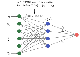
Figure 1: RFFNet as a two-layer neural network. This interpretation is central to foresee extensions of RFFNet beyond the realm of kernel methods.

3.4 Scaling regime for the number of random features

Theoretical properties of random Fourier features have been thoroughly considered recently (Rudi and Rosasco,, 2016; Li et al.,, 2018; Sutherland and Schneider,, 2015). In particular, for learning problems, the focus is on the number of random features needed to attain bounds on the excess risk. Li et al., (2018) showed that $\sqrt{n}\log n$ random features are needed to attain $O(1/\sqrt{n})$ bounds on the excess risk of learning in the squared error loss setting in a worst-case scenario for the regularization parameter. This result has motivated us to heuristically adopt $s=\lfloor\sqrt{n}\log n\rfloor$ as a default value for the number of random Fourier features used, although the user of RFFNet can flexibly set this parameter during the model initialization.

3.5 Extensions

Since RFFNet was developed in a modular fashion with PyTorch (Paszke et al.,, 2019), it seamlessly integrates with other components of this library. In fact, RFFNet can be seen as optimizing the parameters of a two-layer neural network, as depicted in Figure 1, where the connection between the RFF map and the output is done by a linear function. By replacing the link between the RFF map and the output with general neural network architectures, we expect to increase the method’s predictive performance and, most importantly, generate a feature importance metric for neural networks based on the relevances of the ARD kernel. In the same spirit, RFFNet can be used as a layer for any neural network, and thus can be used in a huge variety of tasks, including on unsupervised learning problems.

RFFNet may also be suited for variable selection by introducing a $\ell_{1}$ regularization term associated with the relevances parameter (Brouard et al.,, 2022; Allen,, 2013).

4 Experiments

In this section, we report the results of our empirical evaluation of RFFNet on both synthetic and real-world datasets. We performed hyperparameter tuning for all baseline algorithms, following suggestions of Sculley et al., (2018). Throughout these experiments, we always employ the gaussian kernel with relevances:

$$k(x,y)=e^{-\frac{1}{2}\sum_{i=1}^{p}\lambda_{i}^{2}(x_{i}-y_{i})^{2}}.$$

Baselines

For regression tasks, we compared RFFNet with three baselines: kernel ridge regression (KRR) and bayesian ARD regression (BARD), as implemented in Scikit-learn (Pedregosa et al.,, 2011), and Sparse Random Fourier Feature (SRFF), as implemented by Gregorová et al., (2018). For classification tasks, we compared RFFNet with logistic regression, implemented in Scikit-learn, and XGBoost (Chen and Guestrin,, 2016).

Implementation details

RFFNet is implemented as a PyTorch (Paszke et al.,, 2019) model with a user interface adherent to the standard API of Scikit-learn. This makes the method easily applicable and consistent with other tools available in Scikit-learn, such as hyperparameter searches based on cross-validation. Code is available at https://github.com/mpotto/pyselect.

4.1 Synthetic data

We use synthetic datasets proposed in Gregorová et al., (2018), aiming to evaluate if our approach can correctly identify the relevant features present in the regression function.

SE1

The first experiment from Gregorová et al., (2018) is a regression problem with $p=18$ features of which only $5$ are relevant for the regression function. The response is calculated as $y=\sin[(x_{1}+x_{3})^{2}]\sin(x_{6}x_{7}x_{8})+\varepsilon$ with $\varepsilon\sim\mathsf{Normal}(0,\sigma=0.1)$. We performed two experiments. First, aiming to verify the influence of the sample size on the recovery of relevant features, we trained our model with $10^{3},5\times 10^{3},10^{4}$ and $5\times 10^{4}$ instances. Figure 2 shows that increasing the sample size enhances the identification of relevant features, but even with small sample sizes it can already remove most irrelevant features. Next, to compare with other algorithms, we fix the training size as $n=5\times 10^{4}$ instances and evaluate the performance on a held-out test set with $2\times 10^{3}$ samples. The learning rate and the regularization strength were tuned on a validation set with $2\times 10^{3}$ instances. The adopted loss function was the squared error loss. As shown in Table 2, RFFNet outperformed all baseline algorithms. Importantly, kernel ridge regression could not be trained with $n=5\times 10^{4}$ samples because it exceeded the available RAM memory budget.

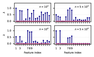
Figure 2: Scaled relevances for the synthetic experiment SE1. Increasing the sample size enhances the identification of relevant features when training RFFNet, but even with small sample sizes RFFNet already gives small weights to most irrelevant features.

SE2

The second experiment is a regression problem with $p=100$ features of which only $5$ are relevant for the regression function. The response is calculated as $y=\log[(x_{11}+x_{12}+x_{13}+x_{14}+x_{15})^{2}]+\varepsilon$ with $\varepsilon\sim\mathsf{Normal}(0,\sigma=0.1)$. The sizes of the training, test, and validation sets are the same as those used in SE1. Again, we performed two experiments, one to verify the effect of sample sizes in the identification of relevant features and the other, with fixed sample size, to compare with baseline algorithms. In both cases, the adopted loss function was the squared error loss. Table 2 shows that, in the fixed sample size scenario, RFFNet outperformed all baseline algorithms. Similarly to the previous experiment, Figure 3 depicts that increasing the sample size strengthen RFFNet ability to identify the relevant features. Moreover, it can already remove most irrelevant features even for small sample sizes.

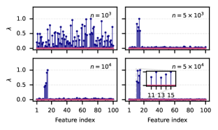
Figure 3: Scaled relevances for the synthetic experiment SE2. Increasing the sample size enhances the identification of relevant features when training RFFNet, but even with small sample sizes RFFNet already gives small weights to most irrelevant features.

4.2 Real-world data

Amazon Fine Food Reviews

This dataset consists of $568,454$ reviews of fine foods sold by Amazon, spanning from October 1999 to October 2012 (McAuley and Leskovec,, 2013). This is a classification task, and the objective is to predict whether a review is positive (has a score between 4 and 5) or negative (has a score between 1 and 3). Information about data processing is available in the Supplementary Material. We used the cross-entropy as the loss function. Table 1 shows that RFFNet performed similarly to the baselines. Additionally, Figure 4 shows that the 10 features (stemmed words) with greater relevances (according to RFFNet) are indeed associated with the quality of the product (e.g. “great”, “best”), while those with smaller relevances are not.

Table 1: Classification metrics in the test set and elapsed time for training RFFNet and baseline algorithms. RFFNet exhibit on par performance with the baselines, but has the advantage of providing feature importances. Best performances are displayed in boldface.

	Amazon					Higgs
$(n,p)$	(291 336, 1000)					(700 000, 28)
Metrics	Acc.	F1	AUC	Time		Acc.	F1	AUC	Time
Logistic	$\mathbf{0.91}$	$\mathbf{0.95}$	$\mathbf{0.94}$	$5.5$ s		$0.64$	$0.69$	$0.68$	$1.3$ s
XGBoost	$0.90$	$0.94$	$0.92$	$111$ s		$\mathbf{0.73}$	$\mathbf{0.75}$	$\mathbf{0.81}$	$52.6$ s
RFFNet	$\mathbf{0.91}$	$\mathbf{0.95}$	$0.93$	$3120$ s		$0.72$	$0.74$	$0.79$	$675$ s

Table 2: Mean squared error in the test set and elapsed time for training RFFNet and baseline algorithms. RFFNet exhibited similar performances in the real-world datasets and outperformed all baselines in the synthetic experiment. OOM indicates that training stopped because the algorithm exceeded the available RAM memory budget. Best performances are displayed in boldface.

	Ailerons			Compact			SE1			SE2
$(n,p)$	$(11\times 10^{3},40)$			$(6\times 10^{3},21)$			$(5\times 10^{4},18)$			$(5\times 10^{4},100)$
Metric	MSE	Time		MSE	Time		MSE	Time		MSE	Time
KRR	$\mathbf{2.4\,(0.3)\times 10^{-8}}$	$12$ s		$\mathbf{9}(2)$	$1.9$ s		OOM	-		OOM	-
BARD	$3.0\,(0.3)\times 10^{-8}$	$0.09$ s		$120\,(50)$	$0.2$ s		$0.088\,(0.008)$	$0.17$ s		$4.9\,(0.5)$	$1.7$ s
SRFF	$8(1)\times 10^{-5}$	$10$ s		$2.5\,(0.4)\times 10^{3}$	$2.9$ s		$0.085\,(0.007)$	$23.9$ s		$5.0\,(0.5)$	$141$ s
RFFNet	$\mathbf{2.7\,(0.3)\times 10^{-8}}$	$768$ s		$\mathbf{10(4)}$	$46$ s		$\mathbf{0.071}\,(0.007)$	$38$ s		$\mathbf{1.2}\,(0.2)$	$462$ s

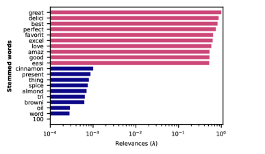
Figure 4: Scaled relevances for the 10 features with greatest (red) and lowest (blue) relevances for the Amazon Fine Food Reviews dataset. The stemmed words with the 10 greatest relevances are indeed associated with product quality, showing that the feature relevance given by RFFNet is meaningful.

Higgs

This dataset is the basis of a classification problem, which aims to distinguish between a signal process associated with the creation of Higgs bosons and a background process that generates similar decay products, but with distinctive features. In this experiment, we used the cross-entropy as the loss function. Table 1 shows that RFFNet performs similarly to baselines. In Figure 5, we compare the feature importances given by RFFNet with the feature importances reported by XGBoost, scaling both to the interval $[0,1]$. Observe that both algorithms give similar relevances to the available features.

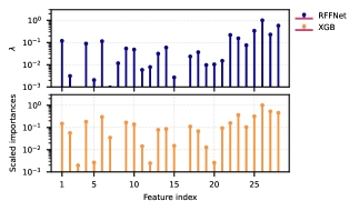
Figure 5: Scaled relevances for RFFNet and XGBoost on the Higgs dataset. Both methods give similar relevances to the available features.

Comp-Act

This dataset consists of a collection of computer systems activity measures. The problem is a regression task and the objective is to predict the portion of time that the CPUs run in user mode, as opposed to system mode (which gives privileged access to hardware). In this case, we used the squared error loss. Table 2 shows that RFFNet performed similarly to other baseline algorithms.

Ailerons

This dataset consists of a collection of sensor measurements describing the status of an F16 aircraft. The goal is to predict the control action on the ailerons of the aircraft. For this dataset, we used the squared error loss. The mean squared error reported in Table 2 shows that RFFNet performance is comparable to the baselines.

5 Conclusions

In this work, we proposed and validated a new scalable and interpretable kernel method, dubbed RFFNet, for supervised learning problems. The method is based on the framework of random Fourier features (Rahimi and Recht,, 2008) applied to ARD kernels. These kernels can be used to assemble kernel methods that are interpretable since the relevances can be used to mitigate the impact of features that do not associate with the response. Besides, the use of random Fourier features diminishes the computational burden of kernel methods (especially their large memory requirements) by reducing the number of parameters to be estimated, thus making our approach scalable.

We validated our approach in a series of numerical experiments, where RFFNet exhibited a performance that is on par with state-of-the-art predictive inference algorithms with a mild requirement on the sample size. In the synthetic datasets, both the predictive performance and identification of relevant features of RFFNet showed promising results. For the real datasets, we observed that RFFNet exhibits a performance that outperforms or is comparable to many commonly used machine learning algorithms.

In future work, we will explore RFFNet for unsupervised problems, as well as its use in the more general architectures discussed in Section 3.5.

Acknowledgments

The authors would like to thank Julio Michael Stern and Roberto Imbuzeiro Oliveira for helpful suggestions. MPO acknowledges financial support through grant 2021/02178-8, São Paulo Research Foundation (FAPESP). RI acknowledges financial support through grants 309607/2020-5 and 422705/2021-7, Brazilian National Counsel of Technological and Scientific Development (CNPq), and grant 2019/11321-9, São Paulo Research Foundation (FAPESP).

References

- Allen, (2013) Allen, G. I. (2013). Automatic feature selection via weighted kernels and regularization. Journal of Computational and Graphical Statistics, 22(2):284–299.
- Bertin and Lecué, (2008) Bertin, K. and Lecué, G. (2008). Selection of variables and dimension reduction in high-dimensional non-parametric regression. Electronic Journal of Statistics, 2(none):1224 – 1241.
- Bolte et al., (2014) Bolte, J., Sabach, S., and Teboulle, M. (2014). Proximal alternating linearized minimization for nonconvex and nonsmooth problems. Math. Program., Ser. A, 146:459–494.
- Bouboulis et al., (2014) Bouboulis, P., Papageorgiou, G., and Theodoridis, S. (2014). Robust image denoising in RKHS via orthogonal matching pursuit. In 2014 4th International Workshop on Cognitive Information Processing (CIP), pages 1–6. IEEE.
- Brouard et al., (2022) Brouard, C., Mariette, J., Flamary, R., and Vialaneix, N. (2022). Feature selection for kernel methods in systems biology. NAR Genomics and Bioinformatics, 4(1).
- Burrows et al., (2019) Burrows, L., Guo, W., Chen, K., and Torella, F. (2019). Edge enhancement for image segmentation using a RKHS method. In Annual Conference on Medical Image Understanding and Analysis, pages 198–207. Springer.
- Chen and Guestrin, (2016) Chen, T. and Guestrin, C. (2016). XGBoost: A scalable tree boosting system. In Proceedings of the 22nd ACM SIGKDD International Conference on Knowledge Discovery and Data Mining, KDD ’16, pages 785–794, New York, NY, USA. ACM.
- Cortes and Vapnik, (1995) Cortes, C. and Vapnik, V. (1995). Support-vector networks. Machine learning, 20(3):273–297.
- Dance and Paige, (2021) Dance, H. and Paige, B. (2021). Fast and scalable spike and slab variable selection in high-dimensional gaussian processes.
- Gregorová et al., (2018) Gregorová, M., Ramapuram, J., Kalousis, A., and Marchand-Maillet, S. (2018). Large-scale nonlinear variable selection via kernel random features.
- Guyon et al., (2002) Guyon, I., Weston, J., Barnhill, S., and Vapnik, V. (2002). Gene selection for cancer classification using support vector machines. Machine learning, 46(1-3):389–422.
- Hofmann et al., (2008) Hofmann, T., Schölkopf, B., and Smola, A. J. (2008). Kernel methods in machine learning. The Annals of Statistics, 36(3).
- Jordan et al., (2021) Jordan, M. I., Liu, K., and Ruan, F. (2021). On the self-penalization phenomenon in feature selection.
- Kadri et al., (2010) Kadri, H., Duflos, E., Preux, P., Canu, S., and Davy, M. (2010). Nonlinear functional regression: a functional RKHS approach. In Proceedings of the Thirteenth International Conference on Artificial Intelligence and Statistics, pages 374–380.
- Keerthi et al., (2006) Keerthi, S., Sindhwani, V., and Chapelle, O. (2006). An efficient method for gradient-based adaptation of hyperparameters in svm models. In Schölkopf, B., Platt, J., and Hoffman, T., editors, Advances in Neural Information Processing Systems, volume 19. MIT Press.
- Kingma and Ba, (2014) Kingma, D. P. and Ba, J. (2014). Adam: A method for stochastic optimization.
- Lafferty and Wasserman, (2008) Lafferty, J. and Wasserman, L. (2008). Rodeo: Sparse, greedy nonparametric regression. The Annals of Statistics, 36(1).
- Li et al., (2018) Li, Z., Ton, J.-F., Oglic, D., and Sejdinovic, D. (2018). Towards a unified analysis of random fourier features. volume 2019-June, pages 6916–6936.
- Louw and Steel, (2006) Louw, N. and Steel, S. (2006). Variable selection in kernel fisher discriminant analysis by means of recursive feature elimination. Computational Statistics & Data Analysis, 51(3):2043–2055.
- McAuley and Leskovec, (2013) McAuley, J. J. and Leskovec, J. (2013). From amateurs to connoisseurs: Modeling the evolution of user expertise through online reviews. In Proceedings of the 22nd International Conference on World Wide Web, WWW ’13, page 897–908, New York, NY, USA. Association for Computing Machinery.
- Mohri et al., (2018) Mohri, M., Rostamizadeh, A., and Talwalkar, A. (2018). Foundations of Machine Learning, second edition. Adaptive Computation and Machine Learning series. MIT Press.
- Oosthuizen, (2008) Oosthuizen, S. (2008). Variable selection for kernel methods with application to binary classification. PhD thesis, Stellenbosch: University of Stellenbosch.
- Paszke et al., (2019) Paszke, A., Gross, S., Massa, F., Lerer, A., Bradbury, J., Chanan, G., Killeen, T., Lin, Z., Gimelshein, N., Antiga, L., et al. (2019). Pytorch: An imperative style, high-performance deep learning library. In Advances in neural information processing systems, pages 8026–8037.
- Pedregosa et al., (2011) Pedregosa, F., Varoquaux, G., Gramfort, A., Michel, V., Thirion, B., Grisel, O., Blondel, M., Prettenhofer, P., Weiss, R., Dubourg, V., Vanderplas, J., Passos, A., Cournapeau, D., Brucher, M., Perrot, M., and Duchesnay, E. (2011). Scikit-learn: Machine learning in Python. Journal of Machine Learning Research, 12:2825–2830.
- Pock and Sabach, (2016) Pock, T. and Sabach, S. (2016). Inertial proximal alternating linearized minimization (iPALM) for nonconvex and nonsmooth problems. SIAM Journal on Imaging Sciences, 9(4):1756–1787.
- Rahimi and Recht, (2008) Rahimi, A. and Recht, B. (2008). Random features for large-scale kernel machines.
- Rasmussen and Williams, (2005) Rasmussen, C. E. and Williams, C. K. I. (2005). Gaussian Processes for Machine Learning (Adaptive Computation and Machine Learning). The MIT Press.
- Rudi et al., (2015) Rudi, A., Camoriano, R., and Rosasco, L. (2015). Less is more: Nyström computational regularization.
- Rudi and Rosasco, (2016) Rudi, A. and Rosasco, L. (2016). Generalization properties of learning with random features.
- Schölkopf and Smola, (2002) Schölkopf, B. and Smola, A. J. (2002). Learning with kernels: Support vector machines, regularization, optimization, and beyond. The MIT Press.
- Sculley et al., (2018) Sculley, D., Snoek, J., Wiltschko, A., and Rahimi, A. (2018). Winner’s curse? on pace, progress, and empirical rigor.
- Shalev-Shwartz and Ben-David, (2014) Shalev-Shwartz, S. and Ben-David, S. (2014). Understanding machine learning: From theory to algorithms. Cambridge University Press.
- Sutherland and Schneider, (2015) Sutherland, D. J. and Schneider, J. (2015). On the error of random fourier features. arXiv preprint arXiv:1506.02785.
- Vaz et al., (2019) Vaz, A. F., Izbicki, R., and Stern, R. B. (2019). Quantification under prior probability shift: the ratio estimator and its extensions. J. Mach. Learn. Res., 20:79–1.
- Wainwright, (2019) Wainwright, M. J. (2019). High-dimensional statistics. Cambridge University Press.
- Xu and Yin, (2014) Xu, Y. and Yin, W. (2014). Block stochastic gradient iteration for convex and nonconvex optimization.
- Zhang, (2006) Zhang, H. H. (2006). Variable selection for support vector machines via smoothing spline anova. Statistica Sinica, pages 659–674.