Gravitational Waves from Feebly Interacting Particles
in a First Order Phase Transition

Abstract

First order phase transitions are well-motivated and extensively studied sources of gravitational waves (GWs) from the early Universe. The vacuum energy released during such transitions is assumed to be transferred primarily either to the expanding walls of bubbles of true vacuum, whose collisions source GWs, or to the surrounding plasma, producing sound waves and turbulence, which act as GW sources. In this Letter, we study an alternative possibility that has so far not been considered: the released energy gets transferred primarily to feebly interacting particles that do not admit a fluid description but simply free-stream individually. We develop the formalism to study the production of GWs from such configurations, and demonstrate that such GW signals have qualitatively distinct characteristics compared to conventional sources and are potentially observable with near-future GW detectors.

I Motivation

Gravitational waves (GWs) provide a unique probe of physics in the early Universe far before Big Bang nucleosynthesis (BBN) and offer a promising window into new physics phenomena at high energy scales. One of the most attractive targets for GW searches is a first order phase transition (FOPT) in the early Universe Hogan (1983); Witten (1984); Hogan (1986); Kosowsky et al. (1992a, b); Kosowsky and Turner (1993); Kamionkowski et al. (1994), where the metastable false vacuum of the early Universe decays through the nucleation, expansion, and percolation of bubbles of true vacuum. The properties of GW signals generated by such FOPTs have been extensively studied in the literature (see e.g.Caprini et al. (2016); Caprini and Figueroa (2018); Caprini et al. (2020); Auclair et al. (2022a) for reviews). While such studies have traditionally focused on the electroweak phase transition (e.g. Grojean and Servant (2007)), FOPTs are more generic and can be realized in a broader class of beyond the Standard Model (BSM) scenarios, where the existence and breaking of additional symmetries in extended sectors (which could include dark/hidden/secluded sectors) is motivated by various shortcomings of the Standard Model (SM). GWs from such dark sector FOPTs are less constrained and can be realized across a broader range of energy scales Schwaller (2015); Jaeckel et al. (2016); Dev and Mazumdar (2016); Baldes (2017); Tsumura et al. (2017); Okada and Seto (2018); Croon et al. (2018); Baldes and Garcia-Cely (2019); Prokopec et al. (2019); Bai et al. (2019); Breitbach et al. (2019); Fairbairn et al. (2019); Helmboldt et al. (2019), offering detection prospects with various current and near future GW detectors such as LIGO-Virgo Abbott et al. (2016a, b), LISA Amaro-Seoane et al. (2017), DECi-hertz Interferometer Gravitational wave Observatory (DECIGO) Kawamura et al. (2006), Big Bang Observer (BBO) Harry et al. (2006), Einstein Telescope (ET) Punturo et al. (2010), and Cosmic Explorer (CE) Reitze et al. (2019).

In FOPTs, GWs are primarily produced in one of two ways. If the bubble walls carry most of the energy released in the phase transition, GWs are sourced by the scalar field energy densities in the bubble walls when the walls collide Kosowsky et al. (1992a, b); Kosowsky and Turner (1993); Kamionkowski et al. (1994); Huber and Konstandin (2008); Bodeker and Moore (2009); Jinno and Takimoto (2017, 2019); Konstandin (2018); Cutting et al. (2018, 2021). In the presence of significant interactions between the bubble walls and the surrounding plasma, the released energy is instead primarily transferred to the plasma, and GWs are produced by sound waves Hindmarsh et al. (2014, 2015, 2017); Cutting et al. (2020); Hindmarsh (2018); Hindmarsh and Hijazi (2019) and turbulence Kamionkowski et al. (1994); Caprini et al. (2009a); Brandenburg et al. (2017); Cutting et al. (2020); Roper Pol et al. (2020); Dahl et al. (2021); Auclair et al. (2022b). These contributions have distinct spectral features determined by the behavior of the bubble walls or sound waves during the percolation phase of the transition.

In this Letter, we study an alternative source of GWs from FOPTs that has so far not been considered in the literature: the energy released in the phase transition can be transferred primarily to feebly-interacting particles (FIPs) that free-stream without interacting over the timescale of the phase transition. Such scenarios can readily occur in dark sectors, which can contain particles with feeble interactions in many realistic scenarios Agrawal et al. (2021). In such cases, bubble walls or sound waves in the plasma carry negligible fractions of the total energy, and cannot be efficient GW sources. It is particularly crucial to explore this possibility, given that it might correspond to a nightmare scenario for GW searches where a FOPT does not lead to observable signals even with otherwise favorable parameters.

We develop the formalism to study the evolution of such FIPs during and after the phase transition. If they are produced or obtain their mass from the FOPT, we find that they form extended noninteracting particle shells that trail the expanding bubble walls; when the bubble walls collide, these particle shells pass through without interacting. We demonstrate that the resulting configurations of overlapping FIP shells produce GWs with distinct characteristics owing to the extended and noninteracting nature of the shells, distinguishing them from conventionally studied GW signals from bubble walls or sound waves. Moreover, we find that these modified GW signals are potentially observable with the next generation of space- and ground-based gravitational wave detectors.

II Framework

We first provide a broad discussion of the general framework for our study. Consider a first order phase transition involving a dark sector scalar $s$ obtaining a vacuum expectation value $\langle s\rangle$ at temperature $T$, which occurs through the nucleation of bubbles of true vacuum (broken phase), whose walls expand into the false vacuum (symmetric phase) with velocity $v_{w}$ (and Lorentz boost factor $\gamma_{w}$). Here $T$ denotes the temperature of the thermal bath with which the scalar field is in equilibrium. In general, $T\lesssim\langle s\rangle$ in most relevant models of thermally triggered phase transitions. For simplicity, we assume that the hidden sector constitutes the dominant form of radiation, and the energy in the Standard Model (SM) bath is negligible.  It is convenient to parametrize the energy density released during the phase transition, given by the difference in the potential energies of the false and true vacua, $\Delta V$, as a fraction of the energy density in the radiation bath 

$$\alpha=\frac{\Delta V}{\rho_{\rm rad}}=\frac{\Delta V}{\frac{\pi^{2}}{30}\,g_{*}^{D}T^{4}}\,,$$ (1)

where $g_{*}^{D}\!=\!g_{\rm bosons}+(7/8)g_{\rm fermions}$ represents the total number of degrees of freedom in the dark sector. We denote the (inverse) timescale for the phase transition to complete by $\beta$, such that $\beta/H$ is the inverse fraction of Hubble time over which the transition completes; for $v_{w}\approx 1$, $\beta$ also represents the average bubble size at collision.

Next, consider a particle $X$ present in the bath that is massless in the false vacuum but obtains a mass $m$ in the true vacuum by virtue of its coupling to $s$. Energy conservation dictates that a massless $X$ particle with energy $E$ in the bath can cross into the bubble wall only if $\gamma_{w}\,E\gtrsim m$. The pressure on the bubble wall  due to a full thermal distribution of particles crossing into the bubble and becoming massive  is Bodeker and Moore (2009) 

$$\mathcal{P}_{\text{max}}\approx\frac{1}{24}m^{2}T^{2}\,.$$ (2)

The free energy released in the transition, $\Delta V_{T}\,(\sim\Delta V)$, does not saturate ${\cal P}_{\rm max}$, i.e. $\Delta V<{\cal P}_{\rm max}$, for

$$m>\sqrt{g_{*}^{D}\alpha}\,T\,,$$ (3)

where we have dropped an $\mathcal{O}(1)$ prefactor for simplicity. In this case, the latent energy released in the transition is entirely absorbed by an appropriate fraction of the $X$ particle population crossing into the bubble walls and becoming massive, and the bubble wall attains a steady-state, terminal velocity.

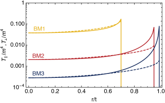
Figure 1: Energy-momentum profile of particles inside an expanding bubble. The solid (dashed) curves denote $T_{\parallel}$ ($T_{\perp}$).

For our numerical studies, we focus on three benchmark (BM) cases:

$$(m/T,v_{w})=\begin{Bmatrix}{\rm BM1}&&{\rm BM2}&&{\rm BM1}\\ (1,0.7)&&(2,0.95)&&(3,0.99)\end{Bmatrix}.$$ (4)

The GW signal we study in this paper is also realized for larger values of $m/T$, with a small fraction of the $X$ particle population entering the bubbles while the majority gets reflected; we choose $m/T\sim 1$ for our benchmark cases purely for convenience as this does not require us to keep track of the reflected population.

Due to the energy transfer from the bubble walls to the particles, the massive $X$ particles in the broken phase gain momenta in the direction of the walls, forming extended shells that trail the bubble walls and expand outwards. Fig. 1 shows the distribution of energy-momentum of particles within a bubble for the BM cases, with the subscripts $\parallel$ and $\perp$ indicating the direction with respect to the wall velocity ($T_{\parallel}=T_{xx}$ and $T_{\perp}=T_{yy}=T_{zz}$ for wall motion in the $x$ direction); see Appendix B for details of the computation, and Eq. 33 for the expression used for the plot. The profiles are found to be self-similar (depending only on $r/t$, the time-dependent bubble radius divided by the time since nucleation), with distributions that are more sharply peaked towards the wall for higher $m/T$ and $\gamma_{w}$, as these are associated with faster walls that can drag the particles along more strongly. Most of the the energy is concentrated in extended shells with thickness comparable to the bubble radius, with a loose tail that extends to the center of the bubble.

We are interested in scenarios where this population of massive particles, or their decay products – we will denote the relevant particle by $Y$ – only have feeble interactions (i.e. effectively do not interact) over the timescale of the phase transition. In the broken phase, $Y$ could interact with other particles in its neighborhood within a bubble during the expansion phase, or with particles inside other bubbles after collision. In both cases, the condition for $Y$ to be noninteracting during the phase transition is

$$n_{Y}\sigma R_{*}<1\,.$$ (5)

Here $n_{Y}$ is the average number density of $Y$ particles (we assume a full thermal distribution enters the bubbles, hence $n_{Y}\sim T^{3}$), $\sigma$ is the relevant interaction cross section, and $R_{*}$, the average bubble size at collision, represents the timescale over which the phase transition completes. If $Y=X$, there are unavoidable $X-s$ and (s-mediated) $X$ self-scattering processes arising from the mass-generating coupling; nevertheless, Eq. 5 can be satisfied with appropriate parameters. Alternatively, if $X$ decays rapidly to other dark sector particles in the broken phase, so that $Y\neq X$, such interactions are trivially avoided. We discuss such model-dependent details of the underlying particle physics model in Appendix A. It should be noted that these massive FIPs $Y$ could account for a significant fraction of the total energy in the Universe; hence we assume that $Y$ is metastable and decays into SM final states after the phase transition completes in order to avoid potential constraints from overclosure.

III Gravitational wave signals

We now discuss the gravitational wave signal generated in the FIP scenario, drawing comparisons with GWs from the more familiar sound wave source. Gravitational waves $h_{ij}$ are the transverse-traceless part of the Friedmann-Lemaître-Robertson-Walker metric $dx^{2}=-dt^{2}+a^{2}(t)(\delta_{ij}+h_{ij})dx^{i}dx^{j}$, sourced by the energy-momentum tensor $T_{\mu\nu}$ through the wave equation $\Box h_{ij}=16\pi G\Lambda_{ij,kl}T_{kl}$, where $\Box$, $G$, and $\Lambda_{ij,kl}$ are the d’Alembertian, the Newtonian constant, and the tensor that projects out the transverse-traceless components, respectively. The GW spectrum $\Omega_{\rm GW}^{*}$ (the superscript denotes that the quantity is calculated at the time of production) is calculated from the Fourier transform of $T_{\mu\nu}$

$$\Omega_{\rm GW}^{*}(k) \equiv\frac{1}{\rho_{\rm tot}}\frac{d\rho_{\rm GW}}{d\ln k}$$

$$\propto\int\frac{d\hat{k}}{4\pi}\Lambda_{ij,kl}(\hat{k})\left.T_{ij}^{*}(\omega,\vec{k})T_{kl}(\omega,\vec{k})\right|_{\omega=|\vec{k}|},$$ (6)

where $\rho_{\rm tot}$ is the total energy density of the Universe at the time of GW production.

In order to calculate the GW production in this system, we develop a novel numerical scheme to calculate the energy-momentum tensor from the superposition of FIPs from multiple bubbles; the details of our calculations and simulations are provided in Appendix B,C,D. We compute GW signals for the case where a bosonic particle $X$ is the FIP, and is thermalized in the symmetric phase. 

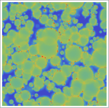
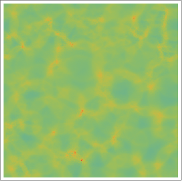
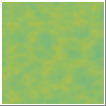
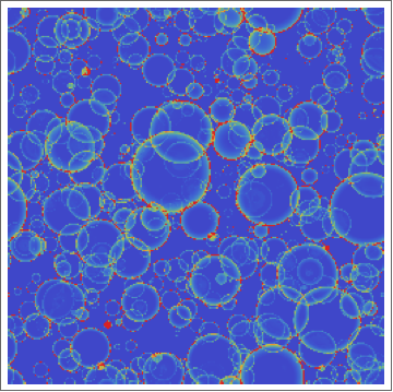
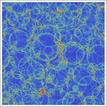
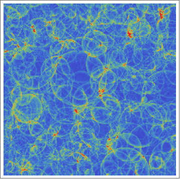
Figure 2: Snapshots of time evolution of $(T_{ij}T_{ij})^{1/4}$ in the FIP scenario (BM1) (top row), contrasted with an analogous simulation in the interacting scenario (sound waves) Jinno et al. (2021) (bottom row). We stress that these plots are meant for illustrative purposes only, to highlight the qualitative differences between the two cases. Blue$\to$green$\to$yellow$\to$red (normalized differently for the two cases) denotes increasing $(T_{ij}T_{ij})^{1/4}$; the red dots in the top row are numerical artifacts.

In Fig. 2, we show snapshots of the time evolution of $(T_{ij}T_{ij})^{1/4}$ from our simulations of FIPs (top row). For comparison, the bottom row shows an analogous simulation (with comparable phase transition parameters and nucleation history) in a setup with sound waves Jinno et al. (2021).  There are two main differences between the two cases. First, as is clearly visible in Fig. 2, the FIP shells extend to the center of the bubble, whereas the sound shells have a clear endpoint corresponding to the sound speed $c_{s}\simeq 1/\sqrt{3}$ determined by hydrodynamics Espinosa et al. (2010); Giese et al. (2020, 2021); Tenkanen and van de Vis (2022). The second concerns the behavior of $T_{ij}$ when the shells cross after bubbles collide. For the FIPs case, since the particles simply free-stream without interacting, the total energy is obtained by simply adding the individual contributions from each bubble

$$T_{ij}(t,\vec{x}) =\sum_{I:~{}{\rm bubbles}}T_{ij}^{(I)}(t,\vec{x}).$$ (7)

Here, it is worth noting that although the shells cross without interacting and superimpose trivially, the spherical symmetry of each shell is nevertheless broken: the shell continues to accumulate more particles in the directions where the expansion is into the symmetric phase (as the FIP particles that are encountered gain mass and get dragged along with the shell) but not in the directions where expansion is into the broken phase (as the particles here are already massive).

In contrast, for the interacting fluid (sound shells), the linearlized fluid equation of motion $(\partial_{t}^{2}-c_{s}^{2}\nabla^{2})v^{\rm(fluid)}_{i}=0$ (with vorticity neglected for simplicity) implies that the fluid velocity field, rather than the energy momentum, superimposes linearly

$$v^{\rm(fluid)}_{i}(t,\vec{x}) =\sum_{I:~{}{\rm bubbles}}v^{{\rm(fluid)}(I)}_{i}(t,\vec{x}).$$ (8)

Consequently, the GW source behaves nonlinearly in the superposition of the fluid shells

$$T^{\rm(fluid)}_{ij}(t,\vec{x}) \sim w(t,\vec{x})v_{i}(t,\vec{x})v_{j}(t,\vec{x})+(\delta_{ij}~{}{\rm piece}),$$ (9)

where $w$ is the fluid’s enthalpy. Due to this nonlinearity, new correlations get imprinted at the scale $k\sim{\rm(shell~{}thickness)}^{-1}$, allowing for the accumulation of GWs at the same scale long after the collisions take place, enhancing the signal by a factor $\lesssim\beta/H$ Hindmarsh et al. (2014, 2015, 2017); Cutting et al. (2020); Hindmarsh (2018); Hindmarsh and Hijazi (2019). The GW signals from FIPs do not feature such correlations, as the particle shell thickness continues to expand as the FIPs propagate; as a consequence, the signal is imprinted over a larger range of wavenumbers, resulting in a broader signal, as we will see below.

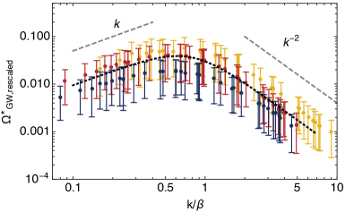
Figure 3: Gravitational wave spectrum rescaled as $\Omega^{*}_{\rm GW}/[(\bar{K}^{(\rm GW)})^{2}(\frac{1}{24}m^{2}T^{2}/\rho_{\rm tot})^{2}(H/\beta)^{2}$]. The dotted black curve shows the broken power law fit $s/(1+s^{3})$. For details of the simulation, see Appendix D (discussion below Eq. 75). The color coding of the BM cases is the same as in Fig. 1.

We simulate the GW signals from FIPs (see Appendix D for details) for the three BM cases (Eq. 4). The signal from our simulation (at production) can be parameterized as

$$\Omega_{\rm GW}^{*}(k) \!\sim\frac{3}{4\pi^{2}}\left(\frac{H}{\beta}\right)^{2}\left(\frac{\frac{1}{24}m^{2}T^{2}}{\rho_{\rm tot}}\right)^{2}\left[\left(\bar{K}^{(\rm GW)}\right)^{2}\,\frac{s}{1+s^{3}}\right],$$ (10)

with $s=0.77\times k/\beta$. Here, note that $\frac{1}{24}m^{2}T^{2}\approx\Delta V$, hence the factor $\left(\frac{\frac{1}{24}m^{2}T^{2}}{\rho_{\rm tot}}\right)^{2}$ represents the characteristic scaling $(\alpha/(1+\alpha))^{2}$ of GW signals, which is also observed for GW signals from sound wave and bubble collision sources (and is also valid in the presence of a SM bath). The part in the square parenthesis is obtained from a fit to the simulation data, and consists of two pieces. The spectral shape is approximately universal, as shown in Fig. 3: the spectra peak at $k\sim 0.77\beta$, and scale as $\sim k^{1}(k^{-2})$ in the IR (UV). In the far IR, we expect the shape to scale as $\sim k^{3}$ as correlations are lost beyond a Hubble time; we do not recover this scaling in our simulations as we ignore the expansion of the Universe.

The function $\bar{K}^{(\rm GW)}$ encodes the details of the underlying process, i.e. the dependence on the parameters $m/T$ and $v_{w}$ or $\gamma_{w}$. It quantifies the fraction of energy in the FIP distribution that is relevant for GW production.  The bar denotes an average over all propagation directions. Its derivation is presented in Appendix D (see text below Eq. 74), but for practical purposes we provide numerical values for various choices of $(m/T,\gamma_{w})$ in Fig. 4. $\bar{K}^{(\rm GW)}$ approaches universal behavior at large $\gamma_{w}$ (see caption). The above fit cannot be used for small $\gamma_{w}$ as $|\bar{K}^{(\rm GW)}|$ features a dip at a particular value of $\gamma_{w}$ for each choice of $m/T$; this originates from the fact that $\bar{K}^{(\rm GW)}$ roughly correlates with the average radial velocity of the particle distribution, and for each $m/T$ there exists a wall velocity for which the particle distribution is approximately static in the plasma frame, making GW production inefficient.

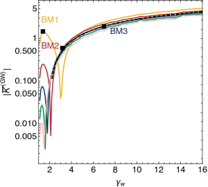
Figure 4: Absolute value of $\bar{K}^{\rm(GW)}$ as a function of $\gamma_{w}$ for $m/T=(1,2,3,4,5)$ (top to bottom). The black dashed curve is a numerical fit with formula $\bar{K}^{\rm(GW)}\sim 12-317/(\gamma_{w}+24)$. The black squares represent our BM points.

To predict the present-day GW signal, Eq. 10 needs to be rescaled by the appropriate redshift factors (see e.g.  Caprini et al. (2020)). In Fig. 5, we plot the resulting GW signals for a few scenarios corresponding to phase transitions at temperatures ranging from $5{\rm\,TeV}$ to $100{\rm\,PeV}$ against the power-law integrated sensitivities of various upcoming space- or ground-based GW detectors. The signal curves constitute of the results of our simulations (colored dots) extrapolated in the UV with a $k^{-2}$-tail, and with a $k^{1}$-tail in the IR, which breaks into a $k^{3}$-tail at the Hubble scale at the time of the transition. If the FIPs decay soon after the phase transition completes, we expect the IR component to shut off exponentially, leaving another characteristic imprint on the signal. For comparison, we also include the GW signal predicted from a sound wave source (blue curve, made with PTPlot Caprini et al. (2020)), with the same phase transition parameters as the blue FIP curve.

The position of the peak of the sound wave signal is set by the size of the sound shells Hindmarsh et al. (2017), whereas the peak of the FIP signal is set by the bubble size, which explains the order of magnitude difference in peak frequency. We see that the amplitude of the GW signal from FIPs is comparable to the sound wave signal: despite the $\beta/H$ enhancement of the latter due to the signal accumulating at the same scale, FIPs appear to be more efficient at sourcing GW signals as there is no energy loss inefficiency due to their noninteracting nature. The plot shows that various upcoming space- or ground-based gravitational wave detectors can be sensitive to FIP-GW signals produced from such phase transitions across a broad range of energy scales. Furthermore, the accumulation of the GW signal over a broader range of wavenumbers also results in the FIP signal having a broader peak that scales as $\sim k^{1}$, which is a distinguishing characteristic of this source that can be used to identify this scenario.

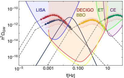
Figure 5: Gravitational wave signals from FIPs with $m/T=3$, $v_{w}=0.99$, and $g_{*}^{D}=5$ (which determine $\alpha=0.23$). The different curves correspond to $T=5~{}{\rm TeV},~{}\beta/H=100$ (blue), $T=5~{}{\rm TeV},~{}\beta/H=50$ (red), $T=1~{}{\rm PeV},~{}\beta/H=100$ (yellow), and $T=100~{}{\rm PeV},~{}\beta/H=50$ (green). For comparison, we also show a sound wave signal (solid curve), using the same phase transition parameters as the blue curve, and $\alpha=0.23$. The power-law integrated sensitivity curves for gravitational wave experiments Harry et al. (2006); Kawamura et al. (2006); Punturo et al. (2010); Amaro-Seoane et al. (2017); Reitze et al. (2019) are for 1 year observation time, with signal-to-noise ratio $=1$, obtained from Schmitz (2021).

IV Discussion

In this Letter, we have discussed a novel source of gravitational wave (GW) signal from a first order phase transition: feebly interacting particles (FIPs) carrying the dominant fraction of the latent energy of the false vacuum released in a phase transition in a dark sector. This provides an interesting and realistic alternative to conventionally studied GW signals from bubble wall collisions and sound waves and turbulence in the plasma, and we have demonstrated that the GW spectra are qualitatively different: compared to a sound wave source with similar phase transition parameters, the FIP-induced signal has comparable amplitude but is broader, and scales differently with frequency. The spectral shape is most similar to that from what is known as the bulk flow model Jinno and Takimoto (2019); Konstandin (2018), which models GW production from thin shells; the crucial difference with our setup is the extended FIP shell thickness, which can imprint distinguishable UV features in the signal. We have also shown that these novel GW signals could be observable in next-generation GW experiments for some benchmark cases. Such FIP configurations appear to be particularly efficient sources of GWs, since there are no energy loss inefficiencies due to their noninteracting nature, and the FIP generated GW signals are comparable in strength to those encountered with sound wave sources.

The qualitative features of the signal we presented here are robust, and the underlying physics well-understood. To avoid the need for numerical simulations to derive the GW signal, we have provided an easy to use analytic formula in Eq. 10 that (in conjunction Fig. 4) can be used to estimate the GW spectra from FIPs in specific BSM models and study the prospects of detection for future experiments.

Several aspects of our results merit further detailed study. We studied a simplified, idealized scenario where the entire energy released in the phase transition goes into FIPs, which act as the only source of GWs. Realistic scenarios likely involve additional features: for instance, a fraction of the particle distribution will get reflected into the false vacuum region; some fraction of the FIPs may in fact self-scatter, or decay into interacting SM states on the same timescale as or shortly after the phase transition. These effects can give rise to sound waves in the plasma, which can act as a secondary source of GWs, while suppressing the signal from FIPs. We estimate that if an $\mathcal{O}(1)$ fraction of the FIPs act in such ways, the resulting sound-wave sourced GW contribution would be of comparable magnitude. Nevertheless, even in such cases, the two contributions can likely be distinguished in an observed signal based on their distinct features (as seen in Fig. 5). Similarly, the case where FIPs produced from the decay of particles crossing into the bubble are significantly lighter than the parent particle will also change the distribution of particles, thus changing the signal; nevertheless, we expect the spectral features to remain the same.

Appendix A Particle Physics Frameworks

The GW signals from feebly interacting particles (FIPs) scenario discussed in this paper requires the dominant fraction of the energy released during a FOPT to be transferred to particles that don’t interact over the timescale of the phase transition, i.e. satisfy Eq. 5. In this appendix, we provide a broad (but not exhaustive) discussion of the particle physics frameworks that could give rise to such setups.

The scalar $s$, which undergoes the phase transition, can itself serve as the FIP if it gains a large mass by virtue of the FOPT; however, a large mass also, in general, implies a large quartic coupling $\lambda_{s}$, which leads to efficient self-scattering in the broken phase. Instead, the role of $X$ can be played by the gauge boson $Z^{\prime}$ corresponding to the broken symmetry; this requires a sufficiently large gauge coupling $g^{\prime}$, such that $m_{Z^{\prime}}=g^{\prime}\langle s\rangle$ saturates the condition in Eq. 3. This coupling $g^{\prime}m_{Z^{\prime}}sZ^{\prime}Z^{\prime}$ can also give rise to scalar-mediated s- and t-channel $Z^{\prime}$ self-scattering processes; assuming $\gamma_{t}T\approx m_{Z^{\prime}}<m_{s}\approx\langle s\rangle$, this self-scattering cross section is $\sigma\sim\frac{g^{\prime 4}}{(4\pi)^{2}}\frac{m_{Z^{\prime}}^{2}}{m_{s}^{4}}$, and the noninteracting condition (Eq. 5) is

$$\frac{(4\pi)^{2}}{g^{\prime 6}}\frac{{\langle s\rangle}^{2}}{T\,M_{Pl}}\frac{\beta}{H}>1\,,$$ (11)

where we have used $R_{*}\approx 1/\beta$, $H\approx T^{2}/M_{Pl}$. For $\beta/H\approx 100$ and $T\sim\mathcal{O}($TeV), this implies $\langle s\rangle/(g^{\prime 2}T)>10^{6}$. Recalling that Eq. 3 also requires $g^{\prime}\,{\langle s\rangle}/T>\mathcal{O}(1)$, satisfying the above condition generally requires $g^{\prime}>0.01,\,\langle s\rangle>100\,T$. In addition, the $Z^{\prime}$ can also scatter with the scalar, but for $m_{s}\approx\langle s\rangle\gg m_{Z},T$ the scalar has a suppressed population in the broken phase, making such scatterings negligible. With this mass hierarchy, inverse decays $Z^{\prime}Z^{\prime}\to s$ and resonant contributions to s-channel $Z^{\prime}$ scattering Frangipane et al. (2022) are also negligible.

Any other particle that gets massive through its coupling to the scalar $s$ will also have similar scattering cross sections mediated by this coupling, and faces similar constraints. Thermally triggered phase transitions generally occur at $T\sim\langle s\rangle$, hence the $\langle s\rangle>100\,T$ hierarchy likely requires some nontrivial setup, such as supercooled transitions Baratella et al. (2019); Delle Rose et al. (2020); Fujikura et al. (2020); Ellis et al. (2019); Brdar et al. (2019); Baldes et al. (2021, 2022), or transition via quantum tunnelling.  We do not pursue the details of such setups further, but simply emphasize the general point that any particle that gets its mass from the phase transition and satisfies Eq. 3 is likely to self-scatter over the course of the phase transition unless $\langle s\rangle\!>\!100\,T$.

Another plausible possibility is that particle $X$ (which could be $s$, $Z^{\prime}$, or some other particle in the dark sector with significant coupling to $s$) decays rapidly into FIPs in the broken phase. As a representative case, consider $Z^{\prime}$ boson decay into a pair of fermions $\psi$ (corresponding to the particle $Y$) in the broken phase, via the interaction $Z^{\prime}\to\psi\bar{\psi}$, with some effective coupling $\epsilon$. Since the massive $Z^{\prime}$ particles move in the plasma with velocities comparable to the wall velocity, the decay rate is $\Gamma_{Z^{\prime}}\approx\frac{\epsilon^{2}}{8\pi\,\gamma_{w}}m_{Z^{\prime}}$. The corresponding decay lifetime is much shorter than the timescale of the phase transition, i.e. $\Gamma_{Z^{\prime}}\gg\beta\sim 1/R_{*}$, provided

$$\epsilon^{2}\gg\frac{8\pi\gamma_{w}}{m_{Z^{\prime}}R_{*}}\approx\frac{8\pi}{\gamma_{w}}\frac{m_{Z^{\prime}}}{M_{Pl}}\frac{\beta}{H}\,,$$ (12)

where we have written $R_{*}\approx 1/\beta$, $H\approx T^{2}/M_{Pl}$, and approximated $\gamma_{w}T\sim m_{Z^{\prime}}$. Note that, in this case, a thermal population of $\psi$ is also likely present in the symmetric phase; these contribute to scattering processes but not the gravitational wave signals if $\psi$ does not gain mass from $\langle s\rangle$.

Again, $\psi$ self-scattering is mediated by $s$- and $t$-channel $Z^{\prime}$ exchange processes, with cross section $\sigma\sim\frac{\epsilon^{4}}{(4\pi)^{2}}\frac{s}{(s-m_{Z^{\prime}}^{2})^{2}+\Gamma_{Z^{\prime}}^{2}m_{Z^{\prime}}^{2}}$ (for $s$-channel) where $\sqrt{s}=E_{cm}$. The collisions typically occur with $E_{cm}\sim\gamma_{w}m_{Z}$, for which $\sigma\sim\frac{\epsilon^{4}}{(4\pi)^{2}}\frac{1}{\gamma_{w}^{2}m_{Z^{\prime}}^{2}}$ (the t-channel cross section is comparable), and the noninteracting condition is 

$$T^{3}\frac{\epsilon^{4}}{(4\pi)^{2}}\frac{1}{\gamma_{w}^{2}m_{Z^{\prime}}^{2}}R_{*}<1\,~{}~{}~{}~{}~{}\Rightarrow~{}~{}~{}~{}~{}\epsilon^{4}<(4\pi)^{2}\gamma_{w}^{3}\frac{m_{Z^{\prime}}}{M_{Pl}}\frac{\beta}{H}\,.$$ (13)

A consistent framework must therefore satisfy Eqs. 3, 12, 13. We find that this is possible in a large region of parameter space; for instance, $\alpha\sim 0.3,\,\gamma_{w}\sim 3,\,\beta/H\sim 100$, $m_{Z^{\prime}}\sim$ TeV, and $\epsilon\sim 10^{-6}-10^{-4}$.

Alternatively, one could also have scenarios where particles that are not originally in the bath get produced efficiently through the interactions of the bubble wall with the plasma through mixing effects, as recently explored in Azatov and Vanvlasselaer (2021); Azatov et al. (2021a, b). While such particles have small number densities compared to thermal abundances, they can be far more massive than the scale of the phase transition, and therefore could carry a large fraction of the energy density released in the course of the phase transition.

In summary, there exist several particle physics frameworks where the energy released in a FOPT could be primarily carried away by FIPs, leading to the production of the GW signals that we have explored in this Letter.

Appendix B Kinematics of particles entering the bubble

Here, we discuss the relations between kinematic properties of a particle before and after entering a bubble. Using unprimed and primed notation for quantities in the symmetric (false vacuum) and broken (true vacuum) phases, the plasma frame energy $E$, four-momentum $p^{\mu}$, and velocity $\vec{v}$ of a particle in the two phases are

$$E=\sqrt{|\vec{p}|^{2}} \equiv p,\qquad E^{\prime}=\sqrt{m^{2}+|\vec{p}^{\prime}|^{2}}\equiv\sqrt{m^{2}+p^{\prime 2}},\qquad\vec{v}=\vec{p}/E,\qquad\vec{v}^{\prime}=\vec{p}^{\prime}/E^{\prime},$$

$$\vec{p} =p_{\parallel}\hat{n}+\vec{p}_{\perp},\qquad\vec{p}^{\prime}=p^{\prime}_{\parallel}\hat{n}+\vec{p}^{\prime}_{\perp},\qquad\text{with}\qquad p_{\parallel}=\vec{p}\cdot\hat{n},~{}p^{\prime}_{\parallel}=\vec{p}^{\prime}\cdot\hat{n},$$ (14)

where $\hat{n}$ is a unit vector orthogonal to the bubble wall pointing outwards. In the wall frame, a particle needs to move towards the bubble, and with sufficient momentum in the $\hat{n}$-direction to enter the bubble and become massive. These conditions correspond to

$$p_{\parallel}-v_{w}E<0,\qquad\gamma_{w}^{2}(p_{\parallel}-v_{w}E)^{2}-m^{2}>0.$$ (15)

We can use energy-momentum conservation (note that momentum is not conserved in the $\hat{n}$ direction) in the wall frame, then boost to the plasma frame to obtain the following relations between the momenta and energies of a particle across the wall:

$$E^{\prime} =\gamma_{w}^{2}(E-v_{w}p_{\parallel})-\gamma_{w}v_{w}\sqrt{\gamma_{w}^{2}(-v_{w}E+p_{\parallel})^{2}-m^{2}},$$ (16)

$$E =\gamma_{w}^{2}(E^{\prime}-v_{w}p_{\parallel}^{\prime})-\gamma_{w}v_{w}\sqrt{\gamma_{w}^{2}(-v_{w}E^{\prime}+p_{\parallel}^{\prime})^{2}+m^{2}},$$ (17)

$$p^{\prime}_{\parallel} =\gamma_{w}^{2}v_{w}(E-v_{w}p_{\parallel})-\gamma_{w}\sqrt{\gamma_{w}^{2}(-v_{w}E+p_{\parallel})^{2}-m^{2}},$$ (18)

$$p_{\parallel} =\gamma_{w}^{2}v_{w}(E^{\prime}-v_{w}p_{\parallel}^{\prime})-\gamma_{w}\sqrt{\gamma_{w}^{2}(-v_{w}E^{\prime}+p_{\parallel}^{\prime})^{2}+m^{2}},$$ (19)

$$\vec{p}_{\perp}^{\prime} =\vec{p}_{\perp}.$$ (20)

Consider a coordinate system where a bubble nucleates at the origin at $t=0$. Given a particle at $(t^{\prime},\vec{x}^{\prime})$ with velocity $v^{\prime}$ inside the bubble, the time $t_{c}$ and position $\vec{x}_{c}$ at which the particle entered the bubble can be evaluated as

$$v_{w}^{2}t_{c}^{2}=|\vec{x}_{c}|^{2},\qquad\vec{x}_{c}=\vec{x}^{\prime}-\vec{v}^{\prime}(t^{\prime}-t_{c}),$$ (21)

which yields

$$t_{c} =\frac{(|\vec{v}^{\prime}|^{2}t^{\prime}-\vec{v}^{\prime}\cdot\vec{x}^{\prime})-\sqrt{(|\vec{v}^{\prime}|^{2}t^{\prime}-\vec{v}^{\prime}\cdot\vec{x}^{\prime})^{2}-(|\vec{v}^{\prime}|^{2}-v_{w}^{2})(|\vec{v}^{\prime}|^{2}t^{\prime 2}-2t^{\prime}\vec{v}^{\prime}\cdot\vec{x}^{\prime}+|\vec{x}^{\prime}|^{2})}}{|\vec{v}^{\prime}|^{2}-v_{w}^{2}}.$$ (22)

Appendix C Energy-momentum tensor of particles in a single bubble

The energy-momentum tensor $T_{ij}$ of particles inside an isolated, expanding bubble is given by

$$T_{ij}(t^{\prime},\vec{x}^{\prime})=\int\frac{d^{3}p^{\prime}}{(2\pi)^{3}}\frac{p^{\prime}_{i}p^{\prime}_{j}}{E^{\prime}}g^{\prime}(t,\vec{x}^{\prime},\vec{p}^{\prime}),$$ (23)

where $g^{\prime}$ is the particle distribution function in the broken phase, which we will determine below. We only consider particles that move towards the bubble wall with sufficient momentum to enter it, ignoring the fraction of the population that gets reflected from the wall. We can write $g^{\prime}(t,\vec{x}^{\prime},\vec{p}^{\prime})=j(\vec{p}^{\prime};\vec{x_{c}})g(t,\vec{x},\vec{p})$, where $g(t,\vec{x},\vec{p})=\frac{1}{e^{E(p^{\prime})/T}\pm 1}$ is the standard distribution (with $E$ determined using Eq. 17), and $j(\vec{p}^{\prime};\vec{x_{c}})$ accounts for any change in the distribution resulting from the particles entering the bubble.

There are, in principle, two different cases to consider:

1. Free-streaming (fs) case: the particles don’t interact in the symmetric phase.

2. Thermalized (th) case: the particles interact efficiently in the symmetric phase, retaining a thermal distribution.

In the free-streaming case, Liouville’s theorem states that the phase space distribution function remains constant along the trajectories of the system, which implies $j_{\rm fs}(\vec{p}^{\prime};\vec{x_{c}})=1$. Thus

$$T_{ij}^{\rm(fs)}(t^{\prime},\vec{x}^{\prime})=\int\frac{d^{3}p^{\prime}}{(2\pi)^{3}}\frac{p^{\prime}_{i}p^{\prime}_{j}}{E^{\prime}}\frac{1}{e^{E(p^{\prime})/T}\pm 1}.$$ (24)

The result can be confirmed by an explicit computation of $g^{\prime}(t,\vec{x}^{\prime},\vec{p}^{\prime})$ via

$$g^{\prime}(t^{\prime},\vec{x}^{\prime},\vec{p}^{\prime})\,dx^{\prime}\wedge dy^{\prime}\wedge dz^{\prime}\wedge dp^{\prime}_{x}\wedge dp^{\prime}_{y}\wedge dp^{\prime}_{z}=g(t,\vec{x},\vec{p})\,dx\wedge dy\wedge dz\wedge dp_{x}\wedge dp_{y}\wedge dp_{z},$$ (25)

where the wedge product relates differential phase-space volume before and after entering the bubble. The distribution functions are related by the determinant $g^{\prime}(t^{\prime},\vec{x},\vec{p}^{\prime})=\left|\det\left[\frac{\partial(x,y,z,p_{x},p_{y},p_{z})}{\partial(x^{\prime},y^{\prime},z^{\prime},p^{\prime}_{x},p^{\prime}_{y},p^{\prime}_{z})}\right]\right|g(t,\vec{x},\vec{p}),$ but we will not provide the details of the computation here.

In the thermalized case, individual particles cannot be tracked in the symmetric phase due to efficient interactions, and Liouville’s theorem cannot be used. We can derive the expression for $j_{\rm th}(\vec{p}^{\prime};\vec{x_{c}})$ by considering the difference between the two cases and using Eq. 25. In the thermalized case, particles undergo multiple scatterings, hence every particle is equally likely to enter the bubble. This is in contrast with the free-streaming case, where particles that move towards the wall with higher velocity enter with a greater flux than slower particles. Particles that move away from the bubble wall with a velocity faster than that of the wall cannot enter at all.

For the free-streaming case, from $\vec{x}=\vec{x}_{c}-\vec{v}(t_{c}-t)$, the differential $d\vec{x}$ at time $t$ is given by $d\vec{x}=d\vec{x}_{c}-d\vec{v}(t_{c}-t)-\vec{v}dt_{c}$. Here $d\vec{v}$ is proportional to $d\vec{p}$ and thus drops out of Eq. 25 because of the wedge product with $dp_{i}$. Using

$$v_{w}^{2}t_{c}^{2}=|\vec{x}_{c}|^{2}\quad\rightarrow\quad dt_{c}=\frac{\vec{x}_{c}\cdot d\vec{x}_{c}}{v_{w}^{2}t_{c}},$$ (26)

we obtain

$$dx\wedge dy\wedge dz\sim\left(1-\frac{\vec{v}\cdot\vec{x}_{c}}{v_{w}^{2}t_{c}}\right)dx_{c}\wedge dy_{c}\wedge dz_{c},$$ (27)

which holds as long as the wedge product with momenta is taken. It can easily be seen that

$$dx_{c}\wedge dy_{c}\wedge dz_{c}\sim\left(1-\frac{\vec{v}^{\prime}\cdot\vec{x}_{c}}{v_{w}^{2}t_{c}}\right)dx^{\prime}\wedge dy^{\prime}\wedge dz^{\prime},$$ (28)

so we arrive at

$$dx\wedge dy\wedge dz\sim\frac{1-\vec{v}\cdot\vec{x}_{c}/v_{w}^{2}t_{c}}{1-\vec{v}^{\prime}\cdot\vec{x}_{c}/v_{w}^{2}t_{c}}\,dx^{\prime}\wedge dy^{\prime}\wedge dz^{\prime}\equiv j_{{\rm fs},x}(\vec{p}^{\prime};\vec{x_{c}})\,dx^{\prime}\wedge dy^{\prime}\wedge dz^{\prime},$$ (29)

where we split $j_{{\rm fs}}$ into space- and momentum-pieces $j_{{\rm fs},x}$ and $j_{{\rm fs},p}$. Note that $j_{{\rm fs},x}$ gets exactly cancelled by $j_{{\rm fs},p}$ relating the primed and unprimed momenta, i.e.

$$j_{\rm fs}(\vec{p}^{\prime};\vec{x_{c}})\equiv j_{{\rm fs},x}(\vec{p}^{\prime};\vec{x_{c}})\times j_{{\rm fs},p}(\vec{p}^{\prime};\vec{x_{c}})=1.$$ (30)

In the thermalized case, we can directly relate $d\vec{x}=d\vec{x}_{c}$ because efficient interactions between particles in the symmetric phase ensure that there is no net flux to/from any volume element in front of the bubble. Therefore

$$dx\wedge dy\wedge dz\sim\frac{1}{1-\vec{v}^{\prime}\cdot\vec{x}_{c}/v_{w}^{2}t_{c}}\,dx^{\prime}\wedge dy^{\prime}\wedge dz^{\prime}\equiv j_{{\rm th},x}(\vec{p}^{\prime};\vec{x_{c}})\,dx^{\prime}\wedge dy^{\prime}\wedge dz^{\prime}.$$ (31)

The factor relating the momenta is unchanged compared to the free-streaming case, i.e. $j_{{\rm fs},p}=j_{{\rm th},p}$, hence

$$j_{\rm th}=j_{\rm fs}\frac{j_{{\rm th},x}}{j_{{\rm fs},x}}=\frac{1}{1-\vec{v}(\vec{p}^{\prime})\cdot\vec{x}_{c}/v_{w}^{2}t_{c}}.$$ (32)

Therefore, the expression for the thermalized case is

$$T_{ij}^{\rm(th)}(t^{\prime},\vec{x}^{\prime})=\int\frac{d^{3}p^{\prime}}{(2\pi)^{3}}\frac{1}{1-\vec{v}(\vec{p}^{\prime})\cdot\vec{x}_{c}/v_{w}^{2}t_{c}}\frac{p^{\prime}_{i}p^{\prime}_{j}}{E^{\prime}}\frac{1}{e^{E(p^{\prime})/T}\pm 1}\,\theta\left[{1-\vec{v}(\vec{p}^{\prime})\cdot\vec{x}_{c}/v_{w}^{2}t_{c}}\right],$$ (33)

where $\theta$ is the Heaviside function.

We use the thermalized case for our studies and simulations. A realistic scenario would lie somewhere in between the two cases; numerically, we find that the resulting GW spectrum is qualitatively similar in both cases.

Appendix D Computation of the gravitational wave spectrum

The result from the previous section, while helpful in determining the single-bubble profile before collision, is not useful for calculating the energy-momentum distribution and the resulting GW signal in many-bubble systems: to apply Eq. 33 to multiple bubbles, for every momentum $\vec{p}^{\prime}$ one has to know all the possible collision points $\vec{x}_{c}$ and the corresponding velocities in the symmetric phase $\vec{v}(\vec{p}^{\prime})$. While this can be done, we employ a different approach that is simpler and more elegant, which we refer to as the sprinkler picture. The main idea (see Fig. 6) is to treat every spatial coordinate as a “sprinkler” that gets turned on when a bubble wall passes through it, emitting a particle spectrum into the broken phase in the direction in which the wall passes. The energy-momentum tensor can then simply be obtained by adding the contributions from all the sprinklers.

D.1 Sprinkler picture

Note that Eq. 33 can be written as

$$T_{ij}(t^{\prime},\vec{x}^{\prime}) =\sum_{{\rm particle}~{}p}\delta^{(3)}\left(\vec{x}^{\prime}-\vec{x}^{\prime(p)}(t^{\prime})\right)\frac{p^{\prime(p)}_{i}p^{\prime(p)}_{j}}{E^{\prime(p)}},$$ (34)

where $\vec{x}^{\prime(p)}(t^{\prime})$ describes the trajectory of a single particle $p$. Since it is practically impossible to track the trajectory of each particle throughout the entire history of the system, we start tracking it just before the particle enters the broken phase. The trajectory inside the bubble is

$$\vec{x}^{\prime(p)}(t^{\prime}) =\vec{x}_{c}+\vec{v}^{\prime}(\vec{p};\vec{x}_{c})(t^{\prime}-t_{c}(\vec{x}_{c})).$$ (35)

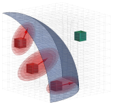
Figure 6: Illustration of the sprinkler picture. The sprinklers in the symmetric/unbroken phase (green cube) are not yet switched on, and contain a thermal distribution of interacting particles. They get switched on (red cubes) when an advancing bubble wall (blue surface) passes through them. The emission of the free-streaming particles from each sprinkler (red ellipses) is determined only by the sprinkler position $\vec{x}_{c}$, the collision time $t_{c}(\vec{x}_{c})$, and the direction $\hat{n}(\vec{x}_{c})$ (red arrow), and is otherwise universal. Since each sprinkler contributes to the energy-momentum tensor linearly, one can first calculate the GW emission from the particles from each sprinkler, then sum these contributions, taking into account the $\vec{x}_{c}$ dependence of each sprinkler.

The next task is to calculate the flux of particles entering the bubble. We approximate the particles in front of the bubble wall with the thermal distribution $1/(e^{E(p)/T}\pm 1)$, neglecting the contribution from reflected components. However, not all particles can enter: some particles are prevented from entering because of the wall potential, while (in the free-streaming case) some particles are moving away from the wall with a velocity greater than the wall velocity. We therefore replace the sum over particles with

$$\sum_{{\rm particle}~{}p} \to\int d^{3}x_{c}\int_{\rm enter}\frac{d^{3}p}{(2\pi)^{3}}\frac{w(\vec{p};\vec{x}_{c})}{e^{E/T}\pm 1},$$ (36)

where $w(\vec{p};\vec{x}_{c})$ is a “wind factor” that accounts for such effects, $\vec{x}_{c}$ is the position where particles cross the wall, and the label ‘enter’ on the integral denotes that we only include particles that have sufficient momentum to enter the bubble. The wind factor for the free-streaming case is defined as $w=j_{{\rm fs},x}/j_{{\rm th},x}$, as needed to compensate for the nontrivial dependence of the volume element and match the result of the previous subsection:

$$w(\vec{p};\vec{x}_{c}) =\left\{\begin{array}[]{cl}1&\quad:\quad{\rm thermalized},\\[14.22636pt] \displaystyle 1-\frac{\vec{v}(\vec{p})\cdot\vec{x}_{c}}{v_{w}^{2}t_{c}}=1-\frac{\vec{v}(\vec{p})\cdot\hat{n}(\vec{x}_{c})}{v_{w}}=1-\frac{\vec{p}\cdot\vec{x}_{c}}{Ev_{w}^{2}t_{c}}&\quad:\quad{\rm free-streaming},\end{array}\right.$$ (39)

where $\vec{p}$ is obtained from $\vec{p}^{\prime}$ via Eqs. 19 and 20. The energy-momentum tensor can then be written as

$$T_{ij}(t^{\prime},\vec{x}^{\prime}) =\int d^{3}x_{c}\int_{\rm enter}\frac{d^{3}p}{(2\pi)^{3}}~{}\delta^{(3)}\left[\vec{x}^{\prime}-(\vec{x}_{c}+\vec{v}^{\prime}(\vec{p};\vec{x}_{c})(t^{\prime}-t_{c}(\vec{x}_{c})))\right]\frac{p_{i}^{\prime}(\vec{p};\vec{x}_{c})p_{j}^{\prime}(\vec{p};\vec{x}_{c})}{E^{\prime}(\vec{p};\vec{x}_{c})}\frac{w(\vec{p};\vec{x}_{c})}{e^{E/T}\pm 1}.$$ (40)

Note that this definition is not restricted to a single bubble but can be applied to a collection of bubbles.

In contrast to the expression in the previous section, we now have integrals over the spatial coordinate $\vec{x}_{c}$ and the momentum $\vec{p}^{\prime}$. The sum over $\vec{x}_{c}$ denotes the sum over sprinklers. Each sprinkler sprays particles when hit by a bubble wall for the first time (see Fig. 6), and is characterized by two quantities:

• $t_{c}(\vec{x}_{c})$: Time when a spatial point $\vec{x}_{c}$ in the symmetric phase first encounters a wall (= sprinkler turned on) .

• $\hat{n}(\vec{x}_{c})$: Direction of wall motion when it passes $\vec{x}_{c}$.

These quantities encode the information about the nucleation history of the collection of bubbles. Note that the sprinklers are universal except for $t_{c}(\vec{x}_{c})$ and $\hat{n}(\vec{x}_{c})$, and, as we will see below, the universal properties of sprinklers are simple to calculate, making the sprinkler approach an efficient way to calculate the GW spectrum from these configurations.

D.2 Gravitational wave spectrum

Gravitational waves, the transverse-traceless components of the metric $ds^{2}=-dt^{2}+a(t)^{2}(\delta_{ij}+h_{ij}(t,\vec{x}))dx^{i}dx^{j}$, are produced through the linearized wave equation of motion in Fourier space

$$\ddot{h}_{ij}(t,\vec{k})+k^{2}h_{ij}(t,\vec{k}) =\frac{2}{M_{P}^{2}}\Lambda_{ij,kl}(\hat{k})T_{kl}(t,\vec{k}).$$ (41)

Here $a(t)$ is the scale factor, $\vec{k}$ is the wave vector of the GWs, the dots indicate time derivatives, $M_{P}\equiv 1/\sqrt{8\pi G}$ is the reduced Planck mass with $G$ being the Newtonian constant, $\Lambda_{ij,kl}(\hat{k})\equiv P_{ik}(\hat{k})P_{jl}(\hat{k})-P_{ij}(\hat{k})P_{kl}(\hat{k})/2$ with $P_{ij}(\hat{k})\equiv\delta_{ij}-\hat{k}_{i}\hat{k}_{j}$ is the projection tensor, and $T_{ij}$ is the energy-momentum tensor. Note that the contraction with $\Lambda_{ij,kl}(\hat{k})$ drops all components irrelevant for GW production. We neglect cosmic expansion, as the phase transition is expected to complete within a small fraction of Hubble time.

The energy density of GWs $\rho_{\rm GW}$ is well-defined once the modes are well inside the horizon, and its logarithmic decomposition can be calculated as Weinberg (1972):

$$\Omega_{\rm GW}^{*}(k) \equiv\frac{1}{\rho_{\rm tot}}\frac{d\rho_{\rm GW}}{d\ln k}=\frac{k^{3}}{4\pi^{2}\rho_{\rm tot}M_{P}^{2}V}\int\frac{d\hat{k}}{4\pi}(\Lambda_{ij,kl}(\hat{k})T_{kl}(\omega=k,\vec{k}))^{*}(\Lambda_{ij,mn}(\hat{k})T_{mn}(\omega=k,\vec{k})),$$ (42)

where integration over $d\hat{k}$ denotes integration over the angular directions and $\rho_{\rm tot}$ and $V$ are the total energy density of the Universe and the volume of the system , respectively. The formula implies that only the Fourier component with $\omega=k\,(\equiv|\vec{k}|)$ contributes to GWs.

To take advantage of the universality of the sprinklers, we will keep $\vec{x}_{c}$ unintegrated in Eq. 40. Taking the Fourier transform of Eq. 40 and omitting the label ‘enter’ for simplicity, we have

$$T_{ij}(\omega=k,\vec{k})= \int d^{3}x_{c}\int\frac{d^{3}p}{(2\pi)^{3}}\int_{t_{c}(\vec{x}_{c})}dt^{\prime}~{}e^{ikt^{\prime}}\int d^{3}x^{\prime}~{}e^{-i\vec{k}\cdot\vec{x}^{\prime}}$$

$$\delta^{(3)}\left[\vec{x}^{\prime}-(\vec{x}_{c}+\vec{v}^{\prime}(\vec{p};\vec{x}_{c})(t^{\prime}-t_{c}(\vec{x}_{c})))\right]\frac{p_{i}^{\prime}(\vec{p};\vec{x}_{c})p_{j}^{\prime}(\vec{p};\vec{x}_{c})}{E^{\prime}(\vec{p};\vec{x}_{c})}\frac{w(\vec{p};\vec{x}_{c})}{e^{E/T}\pm 1}.$$ (43)

We can easily perform the integrals over $\vec{x}^{\prime}$ and $t^{\prime}$. For the latter, we introduce a small imaginary part so that $t^{\prime}\to\infty$ does not contribute. To be more precise, after performing the integration over $\vec{x}^{\prime}$ with the $\delta$-function, we find

$$\int_{t_{c}(\vec{x}_{c})}^{\infty}dt^{\prime}~{}e^{ikt^{\prime}}e^{-i\vec{k}\cdot(\vec{x}_{c}+\vec{v}^{\prime}(\vec{p};\vec{x}_{c})(t^{\prime}-t_{c}(\vec{x}_{c})))} =\int_{0}^{\infty}d(t^{\prime}-t_{c}(\vec{x}_{c}))~{}e^{i(kt_{c}(\vec{x}_{c})-\vec{k}\cdot\vec{x}_{c})}e^{i(k-\vec{k}\cdot\vec{v}^{\prime}(\vec{p};\vec{x}_{c})+i0)(t^{\prime}-t_{c}(\vec{x}_{c}))}$$

$$=\frac{ie^{i(kt_{c}(\vec{x}_{c})-\vec{k}\cdot\vec{x}_{c})}}{k-\vec{k}\cdot\vec{v}^{\prime}(\vec{p};\vec{x}_{c})}.$$ (44)

As this does not take cosmic expansion into account, this assumption breaks down for IR modes $k\lesssim H$. To account for this, we simply change the slope of the GW spectrum at the corresponding wavenumber in our plots to $\Omega_{\rm GW}\propto k^{3}$ Caprini et al. (2009b). We still need to perform the integrals over $\vec{x}_{c}$ and $\vec{p}$. Here, the universality of the sprinklers simplifies the calculation. Using $v^{\prime}_{i}(\vec{p};\vec{x}_{c})=p^{\prime}_{i}(\vec{p};\vec{x}_{c})/E^{\prime}(\vec{p};\vec{x}_{c})$, the projected energy-momentum tensor becomes 

$$\Lambda_{ij,kl}(\hat{k})T_{kl}(\omega=k,\vec{k}) =\int d^{3}x_{c}~{}\frac{ie^{i(kt_{c}(\vec{x}_{c})-\vec{k}\cdot\vec{x}_{c})}}{k}\int\frac{d^{3}p}{(2\pi)^{3}}~{}\frac{\Lambda_{ij,kl}(\hat{k})p_{k}^{\prime}(\vec{p};\vec{x}_{c})p_{l}^{\prime}(\vec{p};\vec{x}_{c})}{E^{\prime}(\vec{p};\vec{x}_{c})-\hat{k}\cdot\vec{p}^{\prime}(\vec{p};\vec{x}_{c})}\frac{w(\vec{p};\vec{x}_{c})}{e^{E/T}\pm 1}.$$ (45)

Note that there are only two explicit parameters $\hat{k}$ and $\hat{n}(\vec{x}_{c})$ in the $\vec{p}$-integrand. The dependence of the primed quantities can be found from the relations in Eqs. 16-20. Taking the tensorial structure into account, we may write

$$\int\!\frac{d^{3}p}{(2\pi)^{3}}\,\frac{p^{\prime}_{i}(\vec{p};\vec{x}_{c})p^{\prime}_{j}(\vec{p};\vec{x}_{c})}{E^{\prime}(\vec{p};\vec{x}_{c})-\vec{p}^{\prime}(\vec{p};\vec{x}_{c})\cdot\hat{k}} \frac{w(\vec{p};\vec{x}_{c})}{e^{E(\vec{p})/T}\pm 1}=$$

$$K_{\delta}\delta_{ij}+K_{kk}\hat{k}_{i}\hat{k}_{j}+K_{kn+nk}(\hat{k}_{i}\hat{n}_{j}(\vec{x}_{c})+\hat{n}_{i}(\vec{x}_{c})\hat{k}_{j})+K_{nn}\hat{n}_{i}(\vec{x}_{c})\hat{n}_{j}(\vec{x}_{c}).$$ (46)

Here $K_{\delta}$, $K_{kk}$, $K_{kn+nk}$, $K_{nn}$ are functions of $\hat{k}\cdot\hat{n}(\vec{x}_{c})$ and model parameters, $K_{\cdots}=K_{\cdots}(\hat{k}\cdot\hat{n}(\vec{x}_{c});v_{w},m,T).$ Thus, for a given set of model parameters, we can first numerically evaluate $K_{\cdots}$ as functions of $\hat{k}\cdot\hat{n}$. Writing $\hat{k}\cdot\hat{n}(\vec{x}_{c})=c$ for simplicity, and contracting with $\delta_{ij}$, $\hat{k}_{i}\hat{k}_{j}$, $\hat{k}_{i}\hat{n}_{j}+\hat{n}_{i}\hat{k}_{j}$, $\hat{n}_{i}\hat{n}_{j}$, respectively, we get

$$\left(\begin{array}[]{c}\int\frac{d^{3}p}{(2\pi)^{3}}~{}\frac{p^{\prime 2}}{E^{\prime}-\vec{p}^{\prime}\cdot\hat{k}}\frac{w}{e^{E/T}+1}\\ \int\frac{d^{3}p}{(2\pi)^{3}}~{}\frac{(\vec{p}^{\prime}\cdot\hat{k})^{2}}{E^{\prime}-\vec{p}^{\prime}\cdot\hat{k}}\frac{w}{e^{E/T}+1}\\ \int\frac{d^{3}p}{(2\pi)^{3}}~{}\frac{2(\vec{p}^{\prime}\cdot\hat{k})(\vec{p}^{\prime}\cdot\hat{n})}{E^{\prime}-\vec{p}^{\prime}\cdot\hat{k}}\frac{w}{e^{E/T}+1}\\ \int\frac{d^{3}p}{(2\pi)^{3}}~{}\frac{(\vec{p}^{\prime}\cdot\hat{n})^{2}}{E^{\prime}-\vec{p}^{\prime}\cdot\hat{k}}\frac{w}{e^{E/T}+1}\end{array}\right) =\left(\begin{array}[]{c c c c}3&1&2c&1\\ 1&1&2c&c^{2}\\ 2c&2c&2(1+c^{2})&2c\\ 1&c^{2}&2c&1\end{array}\right)\left(\begin{array}[]{c}K_{\delta}\\ K_{kk}\\ K_{kn+nk}\\ K_{nn}\end{array}\right).$$ (59)

Inverting this gives

$$\left(\begin{array}[]{c}K_{\delta}\\ K_{kk}\\ K_{kn+nk}\\ K_{nn}\end{array}\right) =\frac{1}{(1-c^{2})^{2}}\left(\begin{array}[]{c c c c}(1-c^{2})^{2}&-(1-c^{2})&c(1-c^{2})&-(1-c^{2})\\ -(1-c^{2})&2&-2c&1+c^{2}\\ c(1-c^{2})&-2c&(1+3c^{2})/2&-2c\\ -(1-c^{2})&1+c^{2}&-2c&2\end{array}\right)\left(\begin{array}[]{c}\int\frac{d^{3}p}{(2\pi)^{3}}~{}\frac{p^{\prime 2}}{E^{\prime}-\vec{p}^{\prime}\cdot\hat{k}}\frac{w}{e^{E/T}\pm 1}\\ \int\frac{d^{3}p}{(2\pi)^{3}}~{}\frac{(\vec{p}^{\prime}\cdot\hat{k})^{2}}{E^{\prime}-\vec{p}^{\prime}\cdot\hat{k}}\frac{w}{e^{E/T}\pm 1}\\ \int\frac{d^{3}p}{(2\pi)^{3}}~{}\frac{2(\vec{p}^{\prime}\cdot\hat{k})(\vec{p}^{\prime}\cdot\hat{n})}{E^{\prime}-\vec{p}^{\prime}\cdot\hat{k}}\frac{w}{e^{E/T}\pm 1}\\ \int\frac{d^{3}p}{(2\pi)^{3}}~{}\frac{(\vec{p}^{\prime}\cdot\hat{n})^{2}}{E^{\prime}-\vec{p}^{\prime}\cdot\hat{k}}\frac{w}{e^{E/T}\pm 1}\end{array}\right).$$ (72)

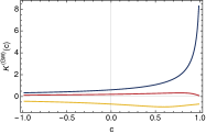
Figure 7: $K^{\rm(GW)}$ as a function of $c=\hat{k}\cdot\hat{n}(\vec{x}_{c})$ for the benchmark scenarios BM1-BM3 (yellow, red, blue).

Of these, only the $K_{nn}$ term survives the projection with $\Lambda_{ij,kl}(\hat{k})$ and is relevant for GW signals, and we accordingly relabel it as $K^{\rm(GW)}$:

$$\Lambda_{ij,kl}(\hat{k})T_{kl}(\omega=k,\vec{k})=\frac{1}{24}m^{2}T^{2}\int d^{3}x_{c}~{}\frac{ie^{i(kt_{c}(\vec{x}_{c})-\vec{k}\cdot\vec{x}_{c})}}{k}\Lambda_{ij,kl}(\hat{k})\hat{n}_{k}(\vec{x}_{c})\hat{n}_{l}(\vec{x}_{c})K^{\rm(GW)}\left(\hat{k}\cdot\hat{n}(\vec{x}_{c})\right),$$ (73)

where

$$K^{\rm(GW)}(c) =\frac{24}{m^{2}T^{2}}\int\frac{d^{3}p~{}}{(2\pi)^{3}}\frac{2(\vec{p}^{\prime}(\vec{p};\vec{x}_{c})\cdot\hat{n}(\vec{x}_{c})-c\hat{k}\cdot\vec{p}^{\prime}(\vec{p};\vec{x}_{c}))^{2}-(1-c^{2})(p^{\prime 2}(\vec{p};\vec{x}_{c})-(\hat{k}\cdot\vec{p}^{\prime}(\vec{p};\vec{x}_{c}))^{2})}{(1-c^{2})^{2}(E^{\prime}(\vec{p};\vec{x}_{c})-\hat{k}\cdot\vec{p}^{\prime}(\vec{p};\vec{x}_{c}))}\frac{w(\vec{p};\vec{x}_{c})}{e^{E/T}\pm 1}.$$ (74)

Note that we have chosen to normalize quantities in terms of $\frac{1}{24}m^{2}T^{2}$, which is the vacuum energy density released during the phase transition, to make a clearer connection to the physical energy scale of the setup. The fact that $K^{\rm(GW)}(c)$ depends on $\vec{x}_{c}$ only through $\hat{n}(\vec{x}_{c})$ is the manifestation of the universality of the sprinklers. $K^{\rm(GW)}(c)$ can thus be determined irrespective of the nucleation history. The $\bar{K}^{\rm(GW)}$ in the fit formula for the GW spectrum in Eq. 10 is precisely this quantity, averaged over its argument $c$.

In Fig. 7, we plot $K^{\rm(GW)}(c)$ for our benchmark scenarios (for the thermalized case). We see that $K^{\rm(GW)}$ is negative for all values of $c$ for BM1 ($(m/T,v_{w})=(1,0.7)$), and (mostly) positive for the other two benchmarks. We find that the value of $K^{\rm(GW)}$ roughly correlates with the average $p^{\prime}_{\parallel}$ of the particles inside the bubble. Note that the gravitational wave spectrum does not depend on the sign of $K^{\rm(GW)}$.

D.3 Procedure to obtain the gravitational wave spectrum

In order to obtain the gravitational wave spectrum, we generate a bubble nucleation history in a box of $V=L^{3}$ with $L=40/\beta$ with the bubble nucleation rate  $\Gamma(t)=\beta^{4}e^{\beta t}$. After nucleation, the bubbles expand with wall velocity $v_{w}$. For each point $x_{c}$ in the box, we determine the time $t_{c}$ at which the first bubble wall passes. In Fig. 8 we show the distribution of the first collision time $t_{c}$ and collision direction $\hat{n}$ (projected onto the 2D plane) in a fixed $z$-slice for a sample simulation.

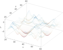
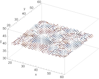
Figure 8: Sample collision data. The left panel is the collision time $t_{c}(\vec{x}_{c})$ between the grid point and the first bubble, while the right panel is the direction of the collision $\hat{n}(\vec{x}_{c})$ (with red and blue indicating upward and downward collisions, respectively). We have plotted data for only a subset of $x$ and $y$ coordinates along a fixed-$z$ slice.

For given $\vec{k}$, we can now calculate the projected tensor $\Lambda_{ij,kl}(\hat{k})T_{kl}(\omega=k,\vec{k})$ from Eq. 73, combining the numerically computed $K^{\rm(GW)}(c)$ (independent of simulations) together with the values of $t_{c}(\vec{x}_{c})$ and $\hat{n}(\vec{x}_{c})$ at each $x_{c}$ obtained from simulations. The gravitational wave spectrum can then be evaluated as

$$\Omega_{\rm GW}^{*}(k)=\frac{3}{4\pi^{2}}\left(\frac{H}{\beta}\right)^{2}\left(\frac{m^{4}}{\rho_{\rm tot}}\right)^{2}\left[\left(\frac{k}{\beta}\right)^{3}\frac{1}{\beta^{3}V}\int\frac{d\hat{k}}{4\pi}\frac{\beta^{4}}{m^{4}}(\Lambda_{ij,kl}(\hat{k})T_{kl}(\omega=k,\vec{k}))^{*}\frac{\beta^{4}}{m^{4}}(\Lambda_{ij,mn}(\hat{k})T_{mn}(\omega=k,\vec{k}))\right],$$ (75)

where the factor in brackets is derived from the simulation. By multiplying the result of the simulation by $(m/T)^{4}$, the relation to Eq. (10) becomes clear.

The GW spectra plotted in Fig. 3 in the main text are obtained from an average of over 50 nucleation history simulations within a box of size $V=L^{3}$ with $L=80v_{w}/\beta$ and periodic boundary conditions. The number of bubbles nucleated is $\sim 20,000$, and we take $N^{3}=256^{3}$ grid points to sample the collision data $t_{c}(\vec{x}_{c})$ and $\hat{n}(\vec{x}_{c})$.

References

- Hogan (1983) C. J. Hogan, Phys. Lett. B 133, 172 (1983).
- Witten (1984) E. Witten, Phys. Rev. D 30, 272 (1984).
- Hogan (1986) C. J. Hogan, Mon. Not. Roy. Astron. Soc. 218, 629 (1986).
- Kosowsky et al. (1992a) A. Kosowsky, M. S. Turner, and R. Watkins, Phys. Rev. D 45, 4514 (1992a).
- Kosowsky et al. (1992b) A. Kosowsky, M. S. Turner, and R. Watkins, Phys. Rev. Lett. 69, 2026 (1992b).
- Kosowsky and Turner (1993) A. Kosowsky and M. S. Turner, Phys. Rev. D 47, 4372 (1993), eprint astro-ph/9211004.
- Kamionkowski et al. (1994) M. Kamionkowski, A. Kosowsky, and M. S. Turner, Phys. Rev. D 49, 2837 (1994), eprint astro-ph/9310044.
- Caprini et al. (2016) C. Caprini et al., JCAP 04, 001 (2016), eprint 1512.06239.
- Caprini and Figueroa (2018) C. Caprini and D. G. Figueroa, Class. Quant. Grav. 35, 163001 (2018), eprint 1801.04268.
- Caprini et al. (2020) C. Caprini et al., JCAP 03, 024 (2020), eprint 1910.13125.
- Auclair et al. (2022a) P. Auclair et al. (LISA Cosmology Working Group) (2022a), eprint 2204.05434.
- Grojean and Servant (2007) C. Grojean and G. Servant, Phys. Rev. D 75, 043507 (2007), eprint hep-ph/0607107.
- Schwaller (2015) P. Schwaller, Phys. Rev. Lett. 115, 181101 (2015), eprint 1504.07263.
- Jaeckel et al. (2016) J. Jaeckel, V. V. Khoze, and M. Spannowsky, Phys. Rev. D 94, 103519 (2016), eprint 1602.03901.
- Dev and Mazumdar (2016) P. S. B. Dev and A. Mazumdar, Phys. Rev. D 93, 104001 (2016), eprint 1602.04203.
- Baldes (2017) I. Baldes, JCAP 05, 028 (2017), eprint 1702.02117.
- Tsumura et al. (2017) K. Tsumura, M. Yamada, and Y. Yamaguchi, JCAP 07, 044 (2017), eprint 1704.00219.
- Okada and Seto (2018) N. Okada and O. Seto, Phys. Rev. D 98, 063532 (2018), eprint 1807.00336.
- Croon et al. (2018) D. Croon, V. Sanz, and G. White, JHEP 08, 203 (2018), eprint 1806.02332.
- Baldes and Garcia-Cely (2019) I. Baldes and C. Garcia-Cely, JHEP 05, 190 (2019), eprint 1809.01198.
- Prokopec et al. (2019) T. Prokopec, J. Rezacek, and B. Świeżewska, JCAP 02, 009 (2019), eprint 1809.11129.
- Bai et al. (2019) Y. Bai, A. J. Long, and S. Lu, Phys. Rev. D 99, 055047 (2019), eprint 1810.04360.
- Breitbach et al. (2019) M. Breitbach, J. Kopp, E. Madge, T. Opferkuch, and P. Schwaller, JCAP 07, 007 (2019), eprint 1811.11175.
- Fairbairn et al. (2019) M. Fairbairn, E. Hardy, and A. Wickens, JHEP 07, 044 (2019), eprint 1901.11038.
- Helmboldt et al. (2019) A. J. Helmboldt, J. Kubo, and S. van der Woude, Phys. Rev. D 100, 055025 (2019), eprint 1904.07891.
- Abbott et al. (2016a) B. P. Abbott et al. (LIGO Scientific, Virgo), Phys. Rev. Lett. 116, 061102 (2016a), eprint 1602.03837.
- Abbott et al. (2016b) B. P. Abbott et al. (LIGO Scientific, Virgo), Phys. Rev. Lett. 116, 241103 (2016b), eprint 1606.04855.
- Amaro-Seoane et al. (2017) P. Amaro-Seoane, H. Audley, S. Babak, J. Baker, E. Barausse, P. Bender, E. Berti, P. Binetruy, M. Born, D. Bortoluzzi, et al., arXiv e-prints arXiv:1702.00786 (2017), eprint 1702.00786.
- Kawamura et al. (2006) S. Kawamura et al., Class. Quant. Grav. 23, S125 (2006).
- Harry et al. (2006) G. M. Harry, P. Fritschel, D. A. Shaddock, W. Folkner, and E. S. Phinney, Class. Quant. Grav. 23, 4887 (2006), [Erratum: Class.Quant.Grav. 23, 7361 (2006)].
- Punturo et al. (2010) M. Punturo et al., Class. Quant. Grav. 27, 194002 (2010).
- Reitze et al. (2019) D. Reitze et al., Bull. Am. Astron. Soc. 51, 035 (2019), eprint 1907.04833.
- Huber and Konstandin (2008) S. J. Huber and T. Konstandin, JCAP 09, 022 (2008), eprint 0806.1828.
- Bodeker and Moore (2009) D. Bodeker and G. D. Moore, JCAP 05, 009 (2009), eprint 0903.4099.
- Jinno and Takimoto (2017) R. Jinno and M. Takimoto, Phys. Rev. D 95, 024009 (2017), eprint 1605.01403.
- Jinno and Takimoto (2019) R. Jinno and M. Takimoto, JCAP 01, 060 (2019), eprint 1707.03111.
- Konstandin (2018) T. Konstandin, JCAP 03, 047 (2018), eprint 1712.06869.
- Cutting et al. (2018) D. Cutting, M. Hindmarsh, and D. J. Weir, Phys. Rev. D 97, 123513 (2018), eprint 1802.05712.
- Cutting et al. (2021) D. Cutting, E. G. Escartin, M. Hindmarsh, and D. J. Weir, Phys. Rev. D 103, 023531 (2021), eprint 2005.13537.
- Hindmarsh et al. (2014) M. Hindmarsh, S. J. Huber, K. Rummukainen, and D. J. Weir, Phys. Rev. Lett. 112, 041301 (2014), eprint 1304.2433.
- Hindmarsh et al. (2015) M. Hindmarsh, S. J. Huber, K. Rummukainen, and D. J. Weir, Phys. Rev. D 92, 123009 (2015), eprint 1504.03291.
- Hindmarsh et al. (2017) M. Hindmarsh, S. J. Huber, K. Rummukainen, and D. J. Weir, Phys. Rev. D 96, 103520 (2017), [Erratum: Phys.Rev.D 101, 089902 (2020)], eprint 1704.05871.
- Cutting et al. (2020) D. Cutting, M. Hindmarsh, and D. J. Weir, Phys. Rev. Lett. 125, 021302 (2020), eprint 1906.00480.
- Hindmarsh (2018) M. Hindmarsh, Phys. Rev. Lett. 120, 071301 (2018), eprint 1608.04735.
- Hindmarsh and Hijazi (2019) M. Hindmarsh and M. Hijazi, JCAP 12, 062 (2019), eprint 1909.10040.
- Caprini et al. (2009a) C. Caprini, R. Durrer, and G. Servant, JCAP 12, 024 (2009a), eprint 0909.0622.
- Brandenburg et al. (2017) A. Brandenburg, T. Kahniashvili, S. Mandal, A. Roper Pol, A. G. Tevzadze, and T. Vachaspati, Phys. Rev. D 96, 123528 (2017), eprint 1711.03804.
- Roper Pol et al. (2020) A. Roper Pol, S. Mandal, A. Brandenburg, T. Kahniashvili, and A. Kosowsky, Phys. Rev. D 102, 083512 (2020), eprint 1903.08585.
- Dahl et al. (2021) J. Dahl, M. Hindmarsh, K. Rummukainen, and D. Weir (2021), eprint 2112.12013.
- Auclair et al. (2022b) P. Auclair, C. Caprini, D. Cutting, M. Hindmarsh, K. Rummukainen, D. A. Steer, and D. J. Weir, JCAP 09, 029 (2022b), eprint 2205.02588.
- Agrawal et al. (2021) P. Agrawal et al., Eur. Phys. J. C 81, 1015 (2021), eprint 2102.12143.
- Giese et al. (2020) F. Giese, T. Konstandin, and J. van de Vis, JCAP 07, 057 (2020), eprint 2004.06995.
- Giese et al. (2021) F. Giese, T. Konstandin, K. Schmitz, and J. van de Vis, JCAP 01, 072 (2021), eprint 2010.09744.
- Bodeker and Moore (2017) D. Bodeker and G. D. Moore, JCAP 05, 025 (2017), eprint 1703.08215.
- Höche et al. (2021) S. Höche, J. Kozaczuk, A. J. Long, J. Turner, and Y. Wang, JCAP 03, 009 (2021), eprint 2007.10343.
- Azatov and Vanvlasselaer (2021) A. Azatov and M. Vanvlasselaer, JCAP 01, 058 (2021), eprint 2010.02590.
- Gouttenoire et al. (2021) Y. Gouttenoire, R. Jinno, and F. Sala (2021), eprint 2112.07686.
- Jinno et al. (2021) R. Jinno, T. Konstandin, and H. Rubira, JCAP 04, 014 (2021), eprint 2010.00971.
- Jinno et al. (2022) R. Jinno, T. Konstandin, H. Rubira, and I. Stomberg (2022), eprint 2209.04369.
- Espinosa et al. (2010) J. R. Espinosa, T. Konstandin, J. M. No, and G. Servant, JCAP 06, 028 (2010), eprint 1004.4187.
- Tenkanen and van de Vis (2022) T. V. I. Tenkanen and J. van de Vis, JHEP 08, 302 (2022), eprint 2206.01130.
- Schmitz (2021) K. Schmitz, JHEP 01, 097 (2021), eprint 2002.04615.
- Frangipane et al. (2022) E. Frangipane, S. Gori, and B. Shakya, JHEP 09, 083 (2022), eprint 2110.10711.
- Baratella et al. (2019) P. Baratella, A. Pomarol, and F. Rompineve, JHEP 03, 100 (2019), eprint 1812.06996.
- Delle Rose et al. (2020) L. Delle Rose, G. Panico, M. Redi, and A. Tesi, JHEP 04, 025 (2020), eprint 1912.06139.
- Fujikura et al. (2020) K. Fujikura, Y. Nakai, and M. Yamada, JHEP 02, 111 (2020), eprint 1910.07546.
- Ellis et al. (2019) J. Ellis, M. Lewicki, J. M. No, and V. Vaskonen, JCAP 06, 024 (2019), eprint 1903.09642.
- Brdar et al. (2019) V. Brdar, A. J. Helmboldt, and M. Lindner, JHEP 12, 158 (2019), eprint 1910.13460.
- Baldes et al. (2021) I. Baldes, Y. Gouttenoire, and F. Sala, JHEP 04, 278 (2021), eprint 2007.08440.
- Baldes et al. (2022) I. Baldes, Y. Gouttenoire, F. Sala, and G. Servant, JHEP 07, 084 (2022), eprint 2110.13926.
- Chu et al. (2014) X. Chu, Y. Mambrini, J. Quevillon, and B. Zaldivar, JCAP 01, 034 (2014), eprint 1306.4677.
- Giudice et al. (2004) G. F. Giudice, A. Notari, M. Raidal, A. Riotto, and A. Strumia, Nucl. Phys. B 685, 89 (2004), eprint hep-ph/0310123.
- Bélanger et al. (2018) G. Bélanger, F. Boudjema, A. Goudelis, A. Pukhov, and B. Zaldivar, Comput. Phys. Commun. 231, 173 (2018), eprint 1801.03509.
- Azatov et al. (2021a) A. Azatov, M. Vanvlasselaer, and W. Yin, JHEP 03, 288 (2021a), eprint 2101.05721.
- Azatov et al. (2021b) A. Azatov, M. Vanvlasselaer, and W. Yin, JHEP 10, 043 (2021b), eprint 2106.14913.
- Weinberg (1972) S. Weinberg, Gravitation and Cosmology: Principles and Applications of the General Theory of Relativity (John Wiley and Sons, New York, 1972), ISBN 978-0-471-92567-5, 978-0-471-92567-5.
- Caprini et al. (2009b) C. Caprini, R. Durrer, T. Konstandin, and G. Servant, Phys. Rev. D 79, 083519 (2009b), eprint 0901.1661.