Neuromorphic Few-Shot Learning: Generalization in Multilayer Physical Neural Networks

Abstract

Neuromorphic computing leverages the complex dynamics of physical systems for computation. The field has recently undergone an explosion in the range and sophistication of implementations, with rapidly improving performance. Neuromorphic schemes typically employ a single physical system, limiting the dimensionality and range of available dynamics - restricting strong performance to a few specific tasks. This is a critical roadblock facing the field, inhibiting the power and versatility of neuromorphic schemes.

Here, we present a solution. We engineer a diverse suite of nanomagnetic arrays and show how tuning microstate space and geometry enables a broad range of dynamics and computing performance. We interconnect arrays in parallel, series and multilayered neural network architectures, where each network node is a distinct physical system. This networked approach grants extremely high dimensionality and enriched dynamics enabling meta-learning to be implemented on small training sets and exhibiting strong performance across a broad taskset. We showcase network performance via few-shot learning, rapidly adapting on-the-fly to previously unseen tasks.

Modern AI and machine-learning provide striking performance, where typically larger models with more dimensions and parameters yield better results. This trend has found empirical support in the study of ‘over-parameterised’ regimes[1, 2], where the number of network parameters greatly surpasses the size of the training dataset. In this regime, models avoid overfitting, generalise well and learn fast with few training data points.

Physical neuromorphic computing, which aims to offload processing for AI problems to the complex dynamics of physical systems[3, 4, 5, 6, 7, 8, 9, 10, 11, 12, 13, 14, 15], stands to benefit considerably from the advantages of operating in an over-parameterised regime. A primary use case of neuromorphic systems is in ‘edge-computing’ where a remotely situated computing and sensing rig locally performs AI-like tasks in a field environment. Here, acquiring large datasets and transmitting them to distant cloud-servers is extremely unattractive, for instance an exoplanet rover vehicle performing object classification[7], making the ability to compute well and adapt to new tasks with small training sets immensely attractive.

However, existing neuromorphic systems tend to have very limited output dimensionality, preventing access to over-parameterised regimes. Neuromorphic systems tend to employ one or $<10$ physical output channels, often current/voltage leads or photodiodes. As these must be physically fabricated, they are challenging to scale, leading to the commonly seen low output dimensional implementations - far from the many thousands of outputs required to access over-parameterisation. In an attempt to remedy this, so-called ‘virtual nodes’ are often implemented[16], repeatedly passing data through a single physical device to artificially enhance dimensionality. This does boost performance but is ultimately limited by the fundamental constraint that network dimensions must be non-degenerate to be computationally useful. As neuromorphic schemes have so far considered single physical systems with a narrow set of defined dynamics, this limit on artificial virtual node dimensionality is highly restrictive.

Neuromorphic computing has been implemented across many physical systems including memristor[17, 18, 19, 20, 21, 22, 23], optical[24] and nanomagnetic systems[25, 26, 27, 28, 29, 30, 5, 31, 32, 33, 14, 34, 35, 36] demonstrating the general performance and scalability of a physical hardware approach[37, 38]. Nanomagnetic systems are attractive, offering solutions to memory volatility and physical degradation issues facing many neuromorphic systems. The magnetic configuration (microstate) provides passive long-term memory. Nanomagnets interact wirelessly through dipolar coupling, allowing spin-wave information transfer with no electron movement and waste heat[39, 40, 41, 42, 12, 11, 43, 44]. Long-range coupling provides passive collective parallel processing[5, 45]. Nanomagnets switch at ns timescales and spin-waves (magnons) offer GHz processing[42, 43, 46, 47, 48, 12, 49, 50, 51, 39, 52, 53]. Crucially, spin-wave spectra offer a route to high-dimensional data output[5, 45] with ferromagnetic resonance spectra providing 100-1000 frequency multiplexed data channels.

However, the reliance on a single set of internal system dynamics results in a lack of versatility and overly-specialised computation in both physical and software-based networks. This arises due to a fundamental compromise between mutually exclusive performance metrics, memory-capacity and nonlinearity[54, 55, 14, 56, 57]. As such, neuromorphic computing schemes relying on single physical systems are constrained to performing well at only a narrow range of tasks. This is a critical barrier facing the field, and until solutions are found neuromorphic computing will remain limited far below its full potential.

In contrast, the brain possesses a rich set of internal dynamics, incorporating multiple memory timescales to efficiently process temporal data[58]. To mimic this, research on software-based reservoirs has shown that combining multiple reservoirs with differing internal dynamics in parallel and series network architectures significantly improves performance[59, 60, 61, 62, 63, 64, 65, 57]. Parallel networks have been physically implemented[66, 67, 8], however they lack inter-node connectivity for transferring information between physical systems - limiting performance. Translating series-connected networks (often termed ‘hierarchical’ or ‘deep’) to physical systems is nontrivial and so-far unrealised due to the large number of possible inter-layer configurations and interconnect complexity.

Here, we present solutions to key outstanding problems in the physical neuromorphic computing field:

• We fabricate three distinct nanomagnetic arrays with different properties and dynamics to explore how physical system design defines computation. (Designing artificial spin reservoirs, Figure 2)

• We develop a methodology to interconnect high-dimensional dynamical systems into networks where nanomagnetic arrays act as complex nodes[68]. Networks show enhanced memory, nonlinearity and task performance beyond any single system. (Multilayer physical neural network, Figure 3)

• We explore network architectures with varying dimensionality. We exploit various learning methodologies for different dimensional regimes. We use feature selection to avoid overfitting in the under-parameterised regime and demonstrate the first realisation of an over-parameterised regime in a physical neuromorphic system, which we showcase via a challenging few-shot learning task using model-agnostic meta-learning[69, 70, 71]. (Multilayer physical neural network, Learning in the over-parameterised regime, Figures 3, 4)

By achieving these milestones, we present a powerful physical computing network which exhibits strong performance across diverse tasks, demonstrating rapid few-shot adaptability to previously unseen tasks. The scheme described here lifts the limitations of low-dimensionality and single physical systems from neuromorphic computing, moving towards a next-generation of powerful, versatile computational networks that harness the synergistic strengths of multiple physical systems.

Network overview

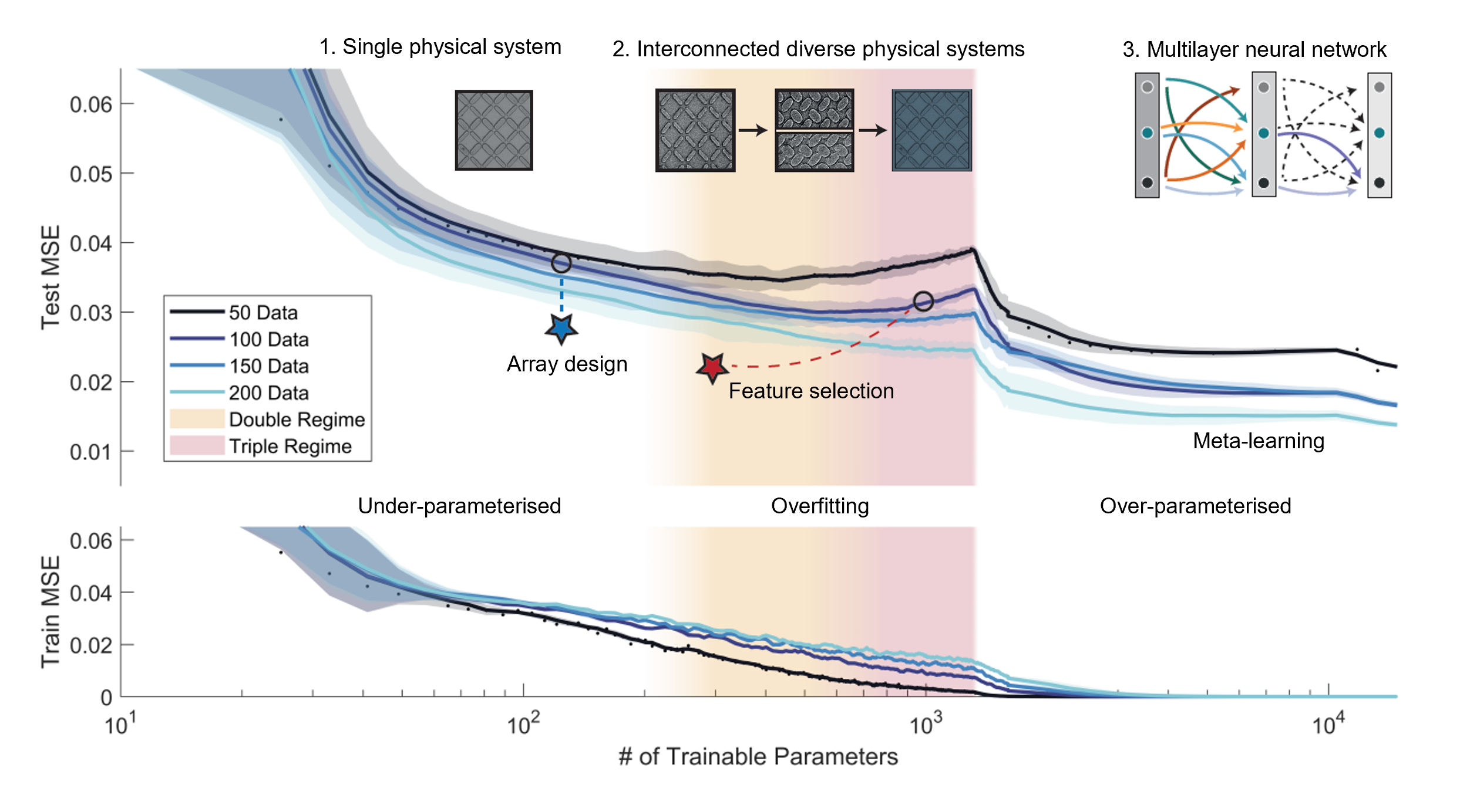
Figure 1: Physical networks explored in this work. Various networks of high-dimensional nanomagnetic arrays are created with increasing number of trainable parameters i.e. system outputs. Dotted lines and stars represent methods of improving computation explored in this work. Curves represent the train and test MSE when predicting the Mackey-Glass time-series while varying the number of network weights and the size of the training data set (colour coded) with shaded regions representing the variation over 10 trials. The curves exhibit the double descent phenomena where MSE follows a ‘U-trend’ in an under-parameterised regime (points 1 and 2). In this regime, we demonstrate how system intelligent array design can be used to enhance spectral richness and improve performance (blue dotted line). Interconnected networks are created to overcome limitations of single arrays (point 2). Orange and purple coloured regions represent networks with two (double) and three (triple) arrays. In this regime MSE increases with increasing parameters due to overfitting. We show how feature selection can be used to reduce the number of outputs whilst improving performance across a broad task set (red dotted line). We then create a physical neural network with complex nodes. In this regime, the system is over-parameterised, enabling significantly enhanced performance and rapid task adaptability through few-shots learning.

We begin by comparing the various physical networks explored in this work. Figure 1 shows schematics of the networks. Points represent the physical network architure. Also shown is the train and test mean-squared-error (MSE) for a chaotic time-series prediction task (Mackey-Glass[72]) across multiple future timescales (discussed later and in the methods section Task selection), when varying the number of trainable parameters (i.e. network output dimensions, x-axis). Dotted lines and star symbols represent methods employed to reduce computational error.

We can broadly classify the observed behaviour into three qualitative regimes, each with a corresponding learning strategy: An initial under-parameterised regime with 10-300 parameters where $N_{trainingdata}>N_{parameters}$, here increasing the number of network parameters monotonically improves performance (left side of Figure 1, point 1. Best performance is obtained designing the most suitable physical array.

When interconnecting physical systems and increasing the number of parameters from 300-1000, the test error of the system follows an expected ‘U-trend’ in an overfitting regime as $N_{trainingdata}\approx N_{parameters}$[73] (middle of Figure 1, point 2). Here, performance deteriorates with increasing network size. The large number of trainable parameters in relation to the size of the training dataset means that there are multiple solutions during training. The network finds one solution resulting in a low train MSE. However, the network has simply memorised the training data and when presented with unseen test data, it fails to accurately predict. This phenomenon gets worse as $N_{parameters}$ increases, up to an extreme where a network can memorise white noise[74] from any training dataset. Good performance may be recovered by employing feature selection strategies to reduce $N_{parameters}$, discussed below.

At 1100 parameters we observed a peak in the test MSE. Surprisingly, as the number of parameters increases ($N_{trainingdata}\ll N_{parameters}$), the test performance substantially improves. Here, we enter an over-parameterised regime and overcome overfitting[75, 73, 1, 2] (right side of Figure 1, point 3). In this regime, instead of simply memorising the training data, the network is able to generalise and learn the underlying behaviour of the task, resulting in strong test performance. Here, multilayered physical neural network architectures are employed where each complex node is a distinct physical system to provide the required high-dimensionality. In this over-parameterised regime very low train and test MSEs are observed. We introduce model-agnostic meta learning (MAML) [71] where the network exhibits the crucial ability to learn with fewer data points. This phenomenon is known in software deep learning (sometimes referred to as a double-descent phenomena[75, 73]), but has not been so-far observed in neuromorphic systems due to their typical low dimensionality.

It should be noted that the transition between regimes depends on both the task, the type of network and the diversity of the trainable system outputs. Furthermore, MSE curves shown in Figure 1 do not represent the absolute best achievable performance, especially in the overfitting region where we later employ feature selection to mitigate overfitting even on smaller network sizes. The curves here are used to illustrate the effect of increasing the number of network parameters without introducing additional learning strategies. Details are given in the methods section Learning algorithms.

Designing artificial spin reservoirs

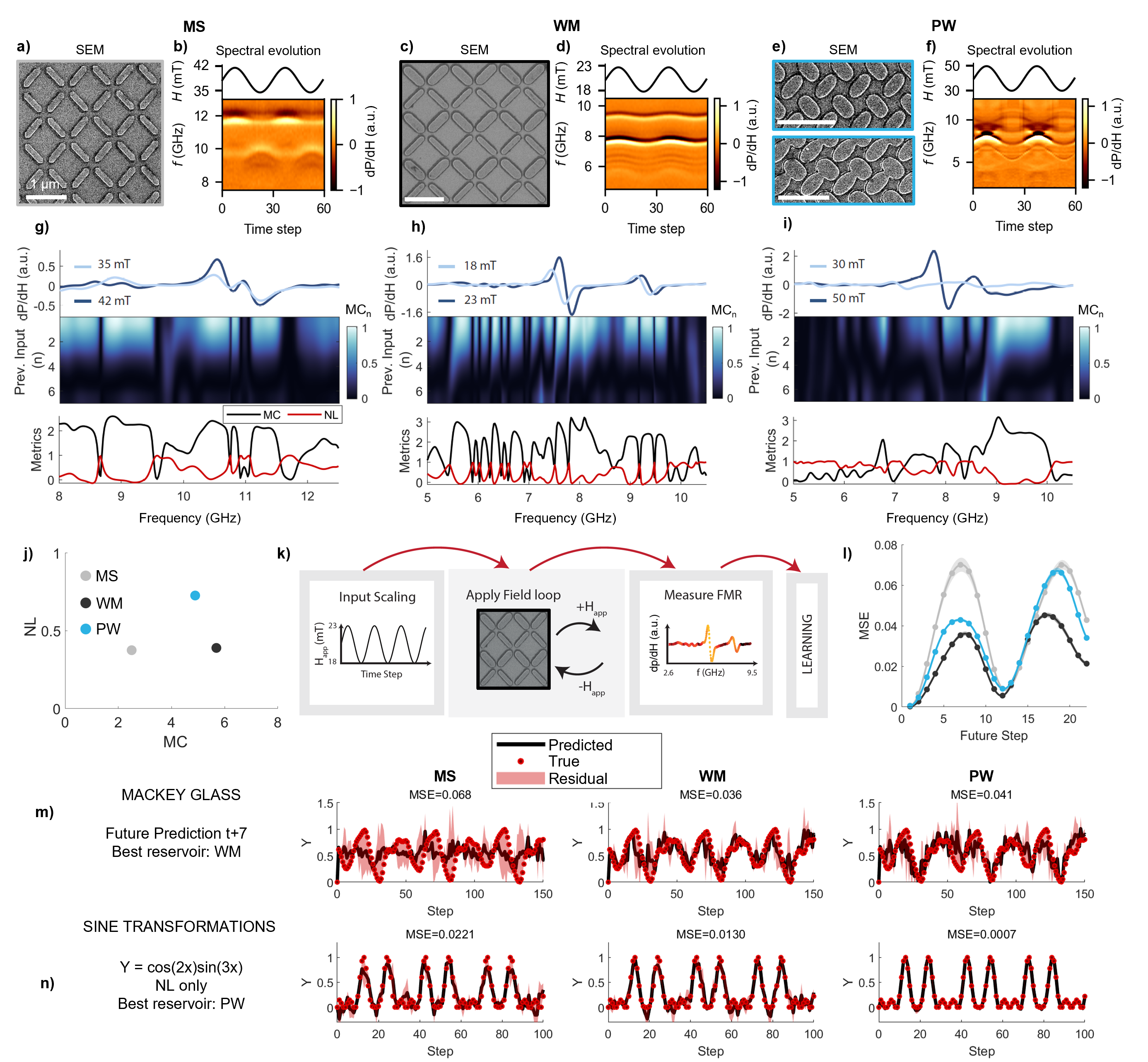
Figure 2: Artificial spin reservoirs. a,b) Square artificial spin ice with macrospin states (MS). c,d) Width-modified square artificial spin-vortex ice (WM). Wide-bars host macrospins and vortices, thin bars just macrospins. e-f) Pinwheel artificial spin-vortex ice (PW). Bars vary from fully disconnected to partially connected and host macrospins and vortices. a,c,e) Scanning electron micrographs. All scale bars correspond to 1 $\mu$m. b,d,f) FMR spectral evolution from a sinusoidal field-series input. MS (g), WM (h) and PW (i) FMR amplitudes at maximum (dark blue) and minimum (light blue) input fields. Frequency-channel signal memory (MC_n) for previous time-steps (n) ranging from 0-7. Memory-capacity (black) and nonlinearity (red) across all output frequencies is shown. MC is a sum of MC_n from n = 0 to 7. j) Memory-capacity (sMC) and nonlinearity (sNL) of the reservoirs. Vortices produce high memory-capacity (WM, PW). Richer FMR spectra produces high nonlinearity (PW). k) Single-reservoir computation schematic. Data is applied via field loops (+H_app then -H_app). FMR output spectra measured at -H_app is used as computational output. l) MSE when predicting future values of the Mackey-Glass time-series. High memory-capacity and low nonlinearity (WM) gives best performance. l) is periodic due to the nature of the Mackey-Glass equation. m,n) Predictions for each reservoir. For challenging prediction tasks (n) no single reservoir performs well.

The relationship between the physical and computational properties of physical systems is central to neuromorphic computing. Here, we examine it by comparing three distinct nanomagnetic ‘artificial spin system’ arrays in a reservoir computing architecture, and develop design rules to enhance and tune computational performance. Previous studies suggest nanomagnetic array geometry and computational capabilities are linked [29] and that the ability to support multiple magnetic textures may play a role in good performance[5], yet the design space remains largely unexplored. Here, we design three distinct arrays to explore a range of magnetic and structural complexity, producing diverse spectral responses and computational capabilities.

The nanomagnetic arrays in this work are based on square and pinwheel artificial spin ice[76]. Figure 2 shows scanning electron micrographs (a,c,e) and spectral evolution of each sample when subject to a sinusoidal field-input (b,d,f). Three arrays were fabricated: MS is a square artificial spin ice (Figure 2 a,b). Bars are high aspect-ratio (530 nm $\times$ 120 nm) and only support macrospin states[5]. WM is a width-modified artificial spin-vortex ice with a subset of wider, lower-coercivity bars (Figure 2 c,d). Bars are 600 nm $\times$ 200 nm (wide-bar)/125 nm (thin-bar). Wide bars host both macrospin and vortex states[5] whereas thin bars host just macrospins. PW is a pinwheel-lattice artificial spin-vortex ice (Figure 2 e,f)[77, 78] with higher density and inter-island coupling. A gradient of bar dimensions are patterned across the sample, ranging from fully-disconnected (e, top) to partially-connected islands (e, bottom) giving a complex range of spectral-responses (Figure 2 f). Bar dimensions are constant across 100 $\times$ 100 $\mu$m² (length 450 nm, width 240 nm / 265 nm (lower / upper panel) in Figure 2 e). Islands support macrospins and vortices. Additional structural and magnetic sample characterisation is shown in supplementary notes 1 $\&$ 2. Fabrication and measurement details are given in the methods section Experimental methods

We assess reservoir performance via two metrics: memory-capacity and nonlinearity. Memory-capacity measures the ability of the current state to recall previous inputs[55], which arises from history-dependent state evolution (i.e. macrospin and vortex conversion). Nonlinearity measures how well past inputs can be linearly mapped to current outputs[55], and can arise from a number of physical system dynamics. In this work, these dynamics include magnon mode-frequency shifts with microstate and input field and the shape of FMR peaks. Metric calculations are further described in the methods section Task selection, and supplementary note 3. Reservoir metrics allow mapping between physical and computational properties, enabling comparison of different systems and revealing how underlying system dynamics define computational properties.

We assess these metrics on a per-output channel basis, highlighting that memory and nonlinearity are provided by distinct spectral channels. Figures 2 g-i) (top) show FMR spectra at max (dark blue) and min (light blue) input field-amplitude, memory-capacity for 0-7 previous time-steps (n) where MC_n is the memory of the nth previous input, total memory-capacity and nonlinearity of each output frequency-channel (bottom). For MS, high MC_n is limited to n $<$ 3. In contrast, WM and PW have some outputs which remember 0-3 prior time-steps and others remembering 4-7 steps (e.g. WM, 7.2 - 7.5 GHz). The presence of multiple memory timescales is provided by vortex dynamics and is key to the strong prediction performance observed later. In PW, the main FMR mode has high nonlinearity due to complex disordered microstate dynamics. The gradient of physical structures in the array provide more non-degenerate nonlinear responses and hence the highest nonlinearity score. Combining the per-channel responses, we can rank each array by a single nonlinearity and memory-capacity metric (Figure 2 j), showing well-separated performances for the three arrays.

We now evaluate the computational performance of each array. Throughout this work, two input datasets are used: a sine-wave and the chaotic Mackey-Glass time-series[72] (described in the methods section Task selection). Figure 2 k) shows a schematic of the single-reservoir computing scheme[5]. Input data is scaled to a suitable field-range to maximise microstate variation. Data is input by applying a minor field-loop, with data value encoded as field-amplitude H_app (i.e. apply field at +H_app then -H_app). Reservoir outputs are obtained by recording FMR spectra at -H_app[5]. We employ short training datasets (250 data points) to reflect real-world applications with strict limitations on data collection time and energy. For single arrays, we operate in the under-paramaterised regime (Figure 1). We employ a feature-selection algorithm selecting the best performing output channels (computational ‘features’ of the network) and discarding unhelpful ones[60, 79] (see methods section Learning algorithms). Performance is evaluated via the MSE between the target and reservoir prediction.

Figure 2 l) shows the performance of each array when predicting various future values (x-axis) of the chaotic time-series. These tasks require high memory-capacity and low nonlinearity, with WM outperforming other arrays. However, all arrays exhibit performance breakdown at harder tasks, evidenced by the periodic MSE profiles in Figure 2 l). This is clear for the prediction of the Mackey-Glass 7 timesteps ahead taken from the high-MSE region (Figure 2 m), here predictions quality is poor with substantial errors. This is a known symptom of single physical systems and software reservoirs which often lack the diverse dynamic timescales necessary to overcome the periodicity of the chaotic dataset and provide a true prediction where performance gradually decreases when predicting further into the future[60, 80, 57]. Performance for a complex history-dependent nonlinear transform task (the NARMA ‘nonlinear autoregressive moving average’ transform[81]) is shown in supplementary note 4 which displays similar behaviour. Figure 2 n) shows signal transformation where a pure sine input signal must be nonlinearly transformed to a complex harmonically-rich signal, here, cos(2x)sin(3x) (further transformations shown in supplementary note 4). PW outperforms MS with 31.6 $\times$ lower MSE, demonstrating the importance of array design optimisation and highlighting the benefit of precisely mapping physical system characteristics to given tasks.

Multilayer physical neural network

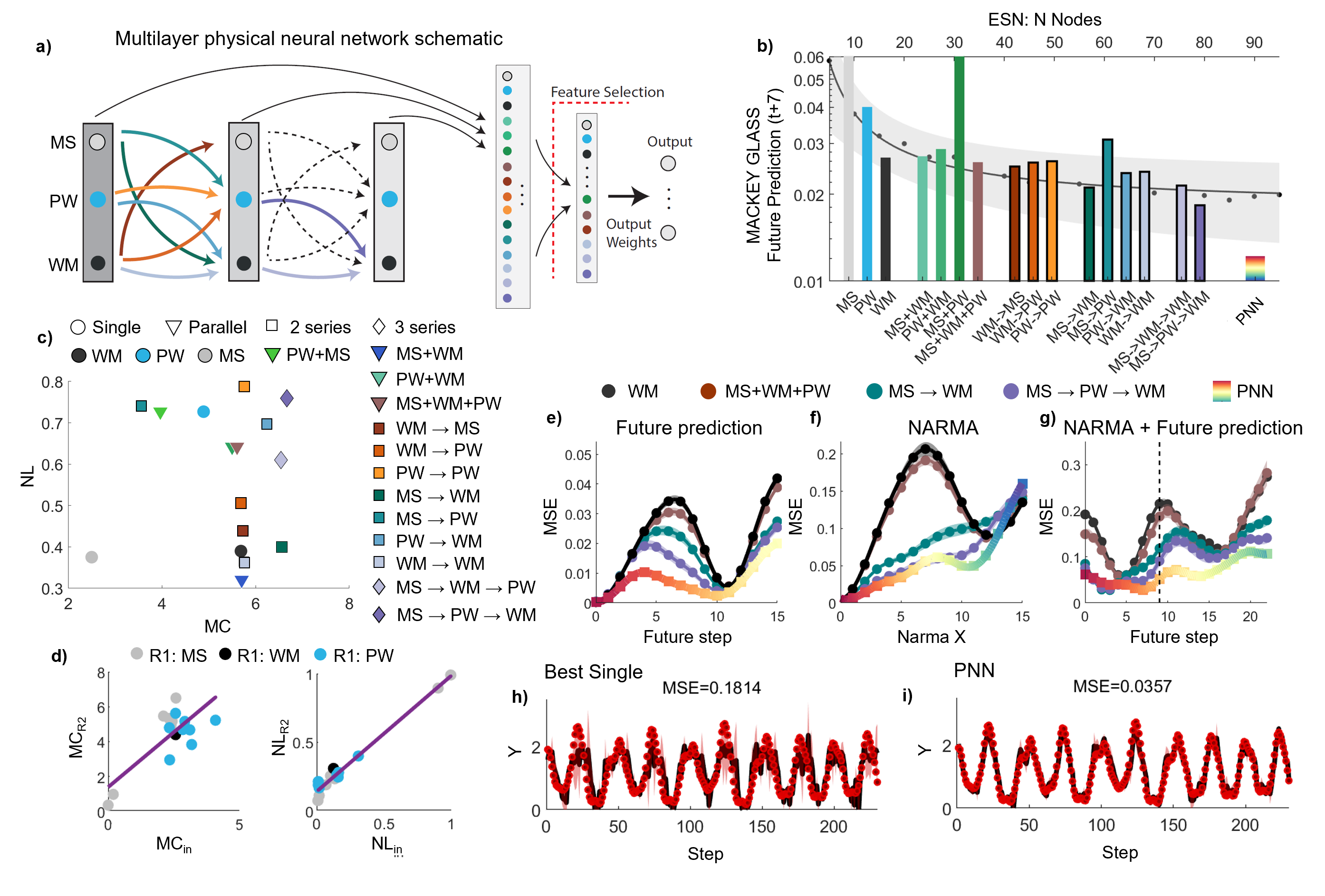
Figure 3: Multilayer physical neural network with reservoir neurons. a) Schematic of the physical neural network system. Multiple series networks, represented by coloured arrows, are combined in parallel. A feature selection algorithm selects outputs across the network to optimise performance. b) MSE when predicting t+7 of the Mackey-Glass equation for single, parallel, series and physical neural network. The neural network shows a significant error reduction. Shaded region and black curve shows the spread and average of MSE’s when using single layer software ESN’s with varying number of network nodes. The neural network achieves significantly better performance whereas single, parallel and deep can be matched by a single ESN. c) Memory-capacity and nonlinearity of single (circles), parallel (triangles) and series networks (squares for series length 2, diamonds for series length 3). A broad range of enhanced memory-capacity and nonlinearities are achieved. PNN’s can take any metric combination. d) Relationship between first reservoir neuron output metrics used for interconnections and measured second reservoir metrics when R2 is WM. Lines represent linear fits. Higher metric scores are correlated with higher-scoring reservoir output channels. MSE profiles for e) Mackey-Glass future prediction, f) NARMA transformation and g) future prediction of NARMA-7 processed Mackey-Glass for the best single, parallel, deep and neural networks. MSE profiles are significantly flattened for the neural network with up to 5.1 $\times$ improvement. h,i) Example predictions for t+9 of the NARMA7 processed Mackey-Glass signal.

The distinct arrays introduced above can each be considered as a complex node or neuron with high memory, nonlinearity and high-dimensionality. We now embed these nodes into a larger physical neural network (PNN). Figure 3 a) shows a schematic of the PNN. The PNN comprises multiple sub-networks where nodes have been connected in series and parallel, represented by coloured arrows. For each sub-network, we map a specific output frequency channel of one node to a field input time-series for the next node and experimentally measure its response (discussed later). For a given combination of nodes, our high output dimensionality enables vast numbers of network architectures to be constructed e.g. MS can be connected to WM by $\sim$ 300 different frequency channels. The PNN explored here comprises 50 two-series and 2 three-series sub-networks. Interconnections between nodes are analogous to programmable network weights, allowing powerful fine-tuning of network performance. Full details of the sub-networks can be found in the methods section Experimental methods and supplementary note 5. The PNN has vast dimensionality with $\sim$16000 features placing it in a over-parameterised regime (Figure 1), previously unexplored in physical neuromorphic systems. We begin by implementing a feature selection scheme [60, 79] to reduce the number of network outputs by discarding less useful channels, avoiding overfitting and providing robust, accurate performance. Here, we use 250 total data points for training and testing. A full description is provided in the methods section Learning algorithms.

To demonstrate the computing power of the physical neural network, we evaluate task-performance across a range of architectures. Figure 3 b) compares from left-to-right on the x-axis: single arrays (MS,PW,WM), parallel networks ($+$ symbol), series networks ($\rightarrow$ symbol) and PNN MSEs for the Mackey-Glass $t$+7 prediction task. The PNN substantially outperforms all other networks considered due to the broad range of memory timescales and nonlinear dynamics present across its constituent complex nodes. As further comparison, the black points and curve show the performance of single layer software echo-state networks (ESNs, see methods section Learning algorithms) with increasing numbers of network nodes (N = 5-100, top x-axis). The grey error margin represents the MSE spread across 100 separate ESN trials with internal ESN network structure randomly initialised each trial. The performance of single, parallel and deep networks can be matched by sufficiently-sized software ESNs. However, the PNN substantially outperforms all single-layer software ESNs considered.

Figure 3 c) shows the memory-capacity and nonlinearity of single, parallel and series sub-networks. Symbols are colour-coded depending on the ordering of complex nodes within the network, consistent with labels in a,b). Parallel network nonlinearity and memory-capacity (triangular markers) scores typically lie between the nonlinearity and memory-capacity from the constituent reservoirs. Memory-capacity does not increase in parallel as no information is directly transferred between network nodes. Series networks (square and diamond symbols for series network depth of 2 and 3 respectively) score highly in nonlinearity and allow memory improvements above any single reservoir. The MS$\rightarrow$PW$\rightarrow$WM network (purple diamond) scores exceptionally well in memory and nonlinearity with correspondingly low MSE. PNN’s can be devised to possess any metric combination. The ordering of arrays in series networks is important, with metric enhancement and lower MSE only observed when networks are sequenced from low (first) to high (last) memory, a phenomenon also seen in software reservoirs[60] and human brains[58].

The significant optimisation time required to evaluate all series architecture interconnections is not practically feasible. For $n$ layers, $N$ complex nodes and $i$ output channels $N^{n\times i}$ configurations are available (here 10²⁸⁶). Instead, we can explore how the output-channel metrics from one reservoir affect the metrics of the next reservoir in a series network. Figure 3 d) shows this relationship when connecting an output from one node (R1) to a second node (R2). Here, the second node is WM (other architectures shown in supplementary note 6). MC_in and NL_in refer to the memory-capacity and nonlinearity of the selected R1 output-channel (i.e. memory-capacity and nonlinearity from Figure 2 panels g-i). MC_R2 and NL_R2 are the memory-capacity and nonlinearity of the second node. Points are colour-coded depending on which array acts as the first node (consistent with previous figures). Both MC_R2 and NL_R2 follow an approximately linear relationship. A linear relationship is also observed when comparing specific previous inputs (supplementary note 6). As such, one may tailor the overall network metrics, and therefore performance, by selecting output-channels with the desired metrics, further demonstrating the efficacy of the per-channel analysis previously presented. We also find that both WM and PW are able to amplify weak amounts of long-term memory in the input signal to give large long-term memory enhancements for the network (supplementary note 6). This interconnection control goes beyond conventional reservoir computing where interconnections are made at random[60], allowing controlled design of network properties.

The PNN outperforms other architectures across all future time step prediction tasks (Figure 3 e) with significant MSE vs $t$ flattening demonstrating higher-quality prediction. This is particularly evident when reconstructing the Mackey-Glass attractor (supplementary note 7). For NARMA transform (Figure 3 f), both the PNN and three-series network show a linear MSE vs $t$ profile, indicative of reaching optimum performance. Reservoir ordering is crucial for series networks with best performance observed when going from low memory to high memory nodes (supplementary note 8). To further test PNN performance, we introduce an additional task - combined nonlinear-transformation and future-prediction using a NARMA-processed Mackey-Glass signal (Figure 3 g). Here, the network is shown the raw Mackey-Glass signal and must predict the future behaviour once it has undergone the complex NARMA nonlinear moving-average transformation. This task requires both high memory and high nonlinearity, with the PNN outperforming all other architectures. Example performance curves when predicting t+9 of the NARMA-processed Mackey-Glass signal is shown for the best single and PNN architectures in Figure 3 h) and i) respectively with the PNN exhibiting far higher performance and better quality signal reconstruction. Additionally, the PNN performs well across a host of nonlinear signal-transformation tasks (Supplementary note 5), outperforming other network architectures at 9/20 tasks. The necessity to match network complexity to task difficulty is well presented here: PNN MSE’s are far closer to those of simpler networks when predicting smaller future step values of Mackey-Glass tasks as well as NARMA processing. A key result of our study here is not only the power of the full 16000 parameter PNN, but the ability to match network size to the task at hand.

Learning in the over-parameterised regime

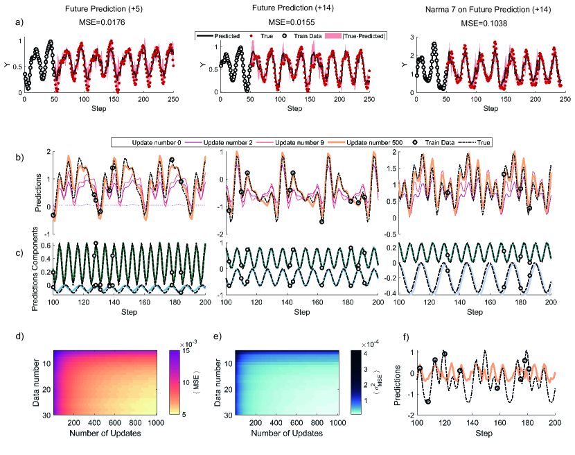
Figure 4: Few-shot learning. a) System predictions (black lines) in the over-parameterised regime when trained on the first 50 data-points (grey circles) of the series. The PNN is able to rapidly learn the task and shows strong performance on the test data set (target points in red). b) Examples of results achieved in the few-shot learning task through meta-learning. The system is asked to learn five different frequency components of a time-varying function (dashed black line). Here, the PNN is shown just 15 training data points (grey circles). As the system is updated, the PNN prediction steadily improves. c) Two example frequency components of the targets in b) which the PNN learns. d) and e) Average error and variance of the error computed over 500 tasks as the number of training data and updates vary. The system shows good generalisation across all tasks as shown by the low error variance. f) Example of prediction from a single reservoir, which fails at the few-shot learning task.

So far, we have explored the performance of different network architectures when trained using a feature-selection algorithm. However, this does not fully showcase the computational advantages of neural networks operating in the over-parameterised regime. The high-dimensionality of the network permits rapid learning with a limited number of data-points[75, 73, 1, 2, 71]. This characteristic is a particularly desirable feature for any neuromorphic computing system as it allows rapid adaptation to changing tasks/environments in remote in-the-field applications where collecting long training datasets carries a high cost. To demonstrate this, we show a challenging fast few-shot learning adaptation for previously unseen tasks using a model-agnostic meta learning approach[69, 71].

Figure 4 a) shows the system prediction when predicting (left-to-right) the $t+5$, $t+14$ and NARMA-processed $t+14$ Mackey-Glass signals. The PNN is trained on just the first 50 data points of the signal, highlighted by black circles. The PNN accomplishes this extremely well with near zero training loss, demonstrating the power and adaptability of the over-parameterised regime. We note that the MSE’s achieved are are comparable to those in Figure 3 e,g) when using feature selection with the PNN. As such, this meta-learning can achieve strong results with a 75$\%$ reduction in training set size (50 training data points here vs 200 previously used).

To further showcase the computational capabilities of the PNN, we now demonstrate few-shot learning where the ‘seen’ training data are sparsely distributed throughout the target dataset, representing for instance a very low sampling rate of a physical input sensor in an edge-computing use-case. In Figure 4 b), the system is driven by a sinusoidal input and asked to predict a target of the form $\tilde{y}(t)=\sum_{n}^{N_{\omega}}a_{n}\sin(nt+\theta_{n})$ i.e. simultaneously predict amplitude, frequency and phase changes - a task that requires a range of temporal dynamics in the network, often used as a meta-learning benchmark task[71]. The values $a_{n}$ and $\theta_{n}$ are sampled randomly at the beginning of each task from continuous uniform distributions (details in the methods section Task selection). The goal is to train the system to generalise to a set of $a_{n}$ and $\theta_{n}$ values, and then rapidly adapt to a new task with only $K$ training points.

In all previous tasks, the network is trained to produce a single output. Here, we simultaneously adapt to five distinct functions and sum the predictions to produce the final waveform. This significantly increases the task difficulty as the network must be generalised to all possible amplitude, frequency and phase shifts, and any errors will be amplified in the final output. To achieve this, we use a variation of the MAML meta-learning algorithm[71] applied to the frequency-channel outputs of the network, leaving all history-dependent and non-linear computation to the intrinsic dynamics of the physical network.

Figure 4 b) and c) show predictions of three example tasks for the overall target and two example sub-components from each task respectively. The network sees just 15 data points (highlighted by grey circles in panel b) throughout the entire process. Figure 4 b) shows the target (dashed black line) and predicted values after updating the generalised matrix a number of times. At update 0, the predicted response does not match the target waveform as expected. As the network updates, the error between the prediction and target reduce. Further example tasks are provided in supplementary note 9.

Despite the limited information and the high variability of tasks, the network can robustly adapt to different targets with the partial information available. As such, the system has learned the underlying sinusoidal components and can rapidly adapt the amplitude, frequency and shift changes for each task. To support this claim of generalisation, Figure 4 d) and e) show the average error and the average variance of the error respectively, calculated over 500 different tasks for various values of $K$ (data number) and number of updates. The error decreases as the number of updates and available data points is increased as expected, with strong performance observed for as little as 10 training data points. Crucially, the variance of the error across all tasks is low, demonstrating strong generalisation. Finally, Figure 4 f) reports an example of prediction obtained when meta-learning is applied on a single reservoir, which fails completely at the task.

The meta-learning approach showcases the richness of the high-dimensional output space of the PNN architecture. The network is able to learn the general behaviour and dynamics of the input and a set of tasks enabling rapid adaptability. This removes the requirement for complete retraining, making essential progress toward on-the-fly system reconfiguration.

Conclusion

We have engineered multiple artificial spin systems with varying microstate dynamics and spin-wave responses, evaluating their metrics and performance across a broad benchmark taskset. Our results highlight the computational performance gained from enriched state spaces, applicable across a broad range of neuromorphic systems. We show the computational benefits of enhanced spatial disorder/parameter gradients and enhanced inter-element coupling in the disordered pinwheel artificial spin reservoir. The PW outperforms MS by up to 31.6$\times$. Our work demonstrates clearly that careful design of system geometry and dynamics is critical, with huge computational benefits available ‘for free’ via physical system design optimisation.

We have overcome the intrinsic performance compromises facing single reservoir systems by engineering network architectures from distinct physical systems. By constructing a physical neural network from a suite of distinct, synergistic physical systems we overcome the fundamental limitation of the memory/nonlinearity tradeoff that currently acts as a roadblock to neuromorphic progress. Additionally, the extremely high dimensionality enabled by the physical neural network architecture allows us to demonstrate the vast benefits of neuromorphic computing in an over-parameterised regime and accomplish demanding and highly-useful few-shot learning tasks with just a handful of distinct physical systems.

The modular, highly-reconfigurable physical neural network architecture pushes neuromorphic computing beyond the limits of simple reservoir computing, enabling strong performance at broader and more challenging tasks and allowing the implementation of modern machine learning approaches such as meta-learning.

Crucially, our efficient method of interconnecting network layers via assessing output-channel/feature metrics allows tailoring of the network metrics, bypassing costly iterative approaches. The approach is broadly-applicable across physical neuromorphic schemes. If the required memory-capacity and nonlinearity for a given task are known, metric programming allows rapid configuration of an appropriate network. If the required memory-capacity and nonlinearity are not known or the task depends on more than these metrics, metric programming can be used to search the memory-capacity, nonlinearity phase space for pockets of high performance. The introduction of a trainable inter-layer parameter opens vast possibilities in implementing hardware neural networks with reservoirs serving as nodes and inter-layer connections serving as weights.

Author contributions

KDS and JCG conceived the work and directed the project throughout.
KDS drafted the manuscript with contributions from all authors in editing and revision stages.
KDS and LM implemented the computation schemes.
LM developed the cross-validation training approach for reducing overfitting on shorter training datasets.
LM developed the feature selection methodology for selecting optimal features from many reservoirs in the multilayer physical neural network architecture.
LM designed and implemented the meta-learning scheme.
KDS designed and implemented the method of interconnecting networks.
CC and TC aided in analysis of reservoir metrics.
KDS, JCG and AV performed FMR measurements.
JCG and HH performed MFM measurements.
JCG and KDS fabricated the samples. JCG and AV performed CAD design of the structures.
JCG performed scanning electron microscopy measurements.
JL contributed task-agnostic metric analysis code.
FC helped with conceiving the work, analysing computing results and providing critical feedback.
EV provided oversight on computational architecture design.
KES and EV provided critical feedback.
WRB oversaw the project and provided critical feedback.

Acknowledgements

This work was supported by the Leverhulme Trust (RPG-2017-257) to WRB and the Engineering and Physical Sciences Research Council (Grant No. EP/W524335/1) to KDS
JCG was supported by the Royal Academy of Engineering under the Research Fellowship programme. AV was supported by the EPSRC Centre for Doctoral Training in Advanced Characterisation of Materials (Grant No. EP/L015277/1).
K.E.S. acknowledges funding from the German Research Foundation (Project No. 320163632) and from the Emergent AI Center funded by the Carl-Zeiss-Stiftung.
The authors would like to thank Hidekazu Kurebayashi for enlightening discussion and feedback and David Mack for excellent laboratory management.

Competing interests

Authors patent applicant. Inventors (in no specific order): Kilian D. Stenning, Jack C. Gartside, Alex Vanstone, Holly H. Holder, Will R. Branford. Application number: PCT/GB2022/052501. Application filed. Patent covers the method of programming deep networks.

Methods

Some description of our methodologies are reproduced from earlier work of several of the authors[45, 5], as similar methods are employed here. The methods section is organised as follows: Experimental Methods includes the fabrication of samples, measurement of FMR response and the details of implementing reservoir computing and interconnecting arrays. Following this we discuss the tasks chosen and how they are evaluated in Task selection. Learning algorithms then provides a detailed description of the learning algorithms used in this work.

Experimental methods

Nanofabrication

Artificial spin reservoirs were fabricated via electron-beam lithography liftoff method on a Raith eLine system with PMMA resist. 25 nm Ni₈₁Fe₁₉ (permalloy) was thermally evaporated and capped with 5 nm Al₂O₃. For WM, a ‘staircase’ subset of bars was increased in width to reduce its coercive field relative to the thin subset, allowing independent subset reversal via global field. For PW, a variation in widths were fabricated across the sample by varying the electron beam lithography dose. Within a 100 $\mu$m $\times$ 100 $\mu$m write-field, the bar dimensions remain constant. The flip-chip FMR measurements require mm-scale nanostructure arrays. Each sample has dimensions of roughly $\sim$ 3x2 mm. As such, the distribution of nanofabrication imperfections termed ‘quenched disorder’ is of greater magnitude here than typically observed in studies on smaller artificial spin systems, typically employing 10-100 micron-scale arrays. The chief consequence of this is that the Gaussian spread of coercive fields is over a few mT for each bar subset. Smaller artificial spin reservoir arrays have narrower coercive field distributions, with the only consequence being that optimal applied field ranges for reservoir computation input will be scaled across a corresponding narrower field range, not an issue for typical 0.1 mT or better field resolution of modern magnet systems.

MFM measurement

Magnetic force micrographs were produced on a Dimension 3100 using commercially available normal-moment MFM tips.

FMR measurement

Ferromagnetic resonance spectra were measured using a NanOsc Instruments cryoFMR in a Quantum Design Physical Properties Measurement System. Broadband FMR measurements were carried out on large area samples $(\sim 3\times 2\leavevmode\nobreak\ \text{ mm}^{2})$ mounted flip-chip style on a coplanar waveguide. The waveguide was connected to a microwave generator, coupling RF magnetic fields to the sample. The output from waveguide was rectified using an RF-diode detector. Measurements were done in fixed in-plane field while the RF frequency was swept in 20 MHz steps. The DC field was then modulated at 490 Hz with a 0.48 mT RMS field and the diode voltage response measured via lock-in. The experimental spectra show the derivative output of the microwave signal as a function of field and frequency. The normalised differential spectra are displayed as false-colour images with symmetric log colour scale[45].

Data input and readout

Reservoir computing schemes consist of three layers: an input layer, a ‘hidden’ reservoir layer, and an output layer corresponding to globally-applied fields, the artificial spin reservoir and the FMR response respectively. For all tasks, the inputs were linearly mapped to a field range spanning 35 - 42 mT for MS, 18 - 23.5 mT for WM and 30-50 mT for PW, with the mapped field value corresponding to the maximum field of a minor loop applied to the system. In other words, for a single data point, we apply a field at +$H_{app}$ then -$H_{app}$. After each minor loop, the FMR response is measured at the applied field -$\mathbf{H}_{\rm app}$ between 8 - 12.5 GHz, 5 - 10.5 GHz and 5 - 10.5 GHz in 20 MHz steps for MS, WM and PW respectively. The FMR output is smoothed in frequency by applying a low-pass filter to reduce noise. Eliminating noise improves computational performance[5]. For each input data-point of the external signal $s(t)$, we measure $\approx 300$ distinct frequency bins and take each bin as an output. This process is repeated for the entire dataset with training and prediction performed offline.

Interconnecting arrays

When interconnecting arrays, we first input the original Mackey-Glass or sinusoidal input into the first array via the input and readout method previously described. We then analyse the memory and non-linearity of each individual frequency output channel (described later). A particular frequency channel of interest is converted to an appropriate field range. The resulting field sequence then applied to the next array via the computing scheme previously described. This process is then repeated for the next array in the network. The outputs from every network layer are concatenated for learning.

Task selection

In the following, we focused on temporally-driven regression tasks that require memory and non-linearity. Considering a sequence of T inputs $\big{[}\mathbf{s}(1),\mathbf{s}(2),...,\mathbf{s}(\rm{T})\big{]}$, the physical system response is a series of observations $\big{[}\mathbf{o}(1),\mathbf{o}(2),...,\mathbf{o}(\rm{T})\big{]}$ across time. These observations can be gathered from a single reservoir configuration as in Figure 2, or can be a collection of activities from multiple reservoirs, in parallel or inter-connected as in Figure 3. In other words, the response of the system $\mathbf{o}(t)$ at time t is the concatenation of the outputs of the different reservoirs used in the architecture considered. The FMR readout characterises the state of each reservoir into approximately 300 features. The tasks faced can be divided into five categories:

• Sine Transformation tasks. The system is driven by a sinusoidal periodic input $s(t)=\sin(t)$ and asked to predict different transformations, such as $\tilde{\mathbf{y}}(t)=\Big{(}|\sin(x/2)|,\sin(2x),\sin(3x),\sin^{2}(x),\sin^{3}(x),\cos(x),\cos(2x),\cos(3x),\rm{saw}(x),\rm{saw}(2x),...\Big{)}$. The inputs $[s(t),s(t+\delta t),...]$ are chosen to have 30 data points per period of the sine, thus with $\delta t=2\pi/30$. The total dataset size is 250 data points. If the target is symmetric with respect to the input, the task only requires nonlinearity. If the target is asymmetric, then both nonlinearity and memory are required.

• Mackey-Glass forecasting. The Mackey-Glass time-delay differential equation takes the form $\dfrac{ds}{dt}=\beta\dfrac{s_{\tau}}{1+s_{\tau}^{n}}-\lambda s$ and is evaluated numerically with $\beta$ = 0.2, n = 10 and $\tau$ = 17. Given $s(t)$ as external varying input, the desired outputs are $\tilde{\mathbf{y}}(t)=\Big{(}s(t+\delta t),s(t+2\delta t),...,s(t+\rm{M}\delta t)\Big{)}$, corresponding to the future of the driving signal at different times. We used 22 data points per period of the external signal for a total of 250 data points. This task predominantly requires memory as constructing future steps requires knowledge of the previous behaviour of the input signal.

• NARMA tasks. Non-linear auto-regressive moving average (NARMA) is a typical benchmark used by the reservoir computing community. The definition of the x-th desired output is $\tilde{y}_{x}(t)=\rm{NARMA}\Big{\{}s(t^{\prime})|x\Big{\}}=As(t^{\prime}-1)+Bs(t^{\prime}-1)\sum_{n=1}^{x}s(t^{\prime}-n)+Cs(t^{\prime}-1)s(t^{\prime}-x)+D$, where the constants were set to the commonly adopted values A = 0.3, B = 0.01, C = 2, D = 0.1. The input signal $s(t^{\prime})$ used is the Mackey-Glass signal, where the variable $t^{\prime}$ is introduced to account for a possible temporal shift of the input. For $t^{\prime}=t$, $\tilde{y}_{x}(t)$ is the application of NARMA on the Mackey-Glass signal at the current time t, while for $t^{\prime}=t+10\delta t$, $\tilde{y}_{x}(t)$ is the result of NARMA on the input signal delayed by ten time steps in the future. The index $x$ can instead vary between one, defining a task with a single temporal dependency, and fifteen, for a problem that requires memory of fifteen inputs. Varying $x$ and $t^{\prime}$, we can define a rich variety of tasks with different levels of difficulty.

• Evaluations of memory-capacity (MC) and non-linearity (NL). Memory capacity and non-linearity are metrics frequently used for the characterization of the properties of a physical device. While these metrics do not constitute tasks in the common terminology, we include them in this section for simplicity of explanation. Indeed, we used the same training methodology to measure MC and NL as in the other tasks faced. We evaluate these metrics with the Mackey-Glass time-delay differential equation as input. This gives results that are correlated to conventional memory-capacity and nonlinearity scores, with some small convolution of the input signal - negligible for our purposes of relatively assessing artificial spin reservoirs and designing network interconnections.
  For memory-capacity the desired outputs are $\tilde{\mathbf{y}}(t)=\Big{(}s(t-\delta t),s(t-2\delta t),...,s(t-\rm{k}\delta t)\Big{)}$, corresponding to the previous inputs of the driving signal at different times. To avoid effects from the periodicity of the input signal, we set k=8. The R² value of the predicted and target values is evaluated for each value of $\delta t$ where a high R² value means a good linear fit and high memory and a low R² value means a poor fit a low memory. The final memory-capacity value is the sum of R² from $k$ = 0 to $k$ = 8.
  For nonlinearity, $\mathbf{x}(t)$ is the input signal from t = 0 to t = -7 and $\tilde{\mathbf{y}}(t)$ is a certain reservoir output. For each output, the R² value of the predicted and target values is evaluated. Nonlinearity for a single output is given by 1 - R² i.e. a good linear fit gives a high R² and low nonlinearity and a bad linear fit gives low R² and high nonlinearity. Nonlinearity is averaged over all selected features.
  Memory capacity and non-linearity can be calculated using a single or multiple frequency channels.

• Frequency decomposition, a few-shot learning task. The network is driven by a sinusoidal input $s(t)$ and needs to reconstruct a decomposition of a temporal varying signal in the form of $\sum_{n}^{N_{\omega}}a_{n}\sin(nt+\theta_{n})$, where $N_{\omega}=5$. The values of $a_{n}$ and $\theta_{n}$ are randomly sampled at the beginning of each task from uniform distributions. In particular, $a_{n}\in[-1.2\ \ 1.2]$ and $\theta_{n}\in[0\ \ \pi/n]$. The output layer is composed of $N_{\omega}$ nodes, and the system is asked to predict a target $\tilde{\mathbf{y}}(t)=\Big{(}a_{1}sin(t+\theta_{1}),a_{2}sin(2t+\theta_{2}),...,a_{5}sin(5t+\theta_{5})\Big{)}$ after observing the values of $\tilde{\mathbf{y}}(t)$ over K data points, that is different time steps. The value of K adopted for the examples of Figure 4 b) and c) is fifteen, but the network reports good performance even with $\rm{K}=10$ (Figure 4 d) and e). To face this challenging task, we used the network in the over-parameterised regime and a meta-learning algorithm to quickly adapt the read-out connectivity. Details of the meta-learning approach are given below in the Meta-learning section of the Methods.

Learning algorithms

For comparisons between different systems, training is accomplished through a features selection algorithm (discussed below) and optimisation of the read-out weights $\mathbf{W}_{o}$. We call $\mathbf{x}(t)$ the representation at which the read-out weights operate after the application of feature-selection, and we define the output of the system as $\mathbf{y}(t)=\mathbf{W}_{o}\mathbf{x}(t)$. Of course, $\mathbf{x}(t)$ simply contains a subset of features of $\mathbf{o}(t)$. In this setting, optimisation of $\mathbf{W}_{o}$ is achieved with ridge regression, which minimises the error function $\rm{E}=\sum_{t}||\tilde{y}(t)-\mathbf{W}_{o}\mathbf{x}(t)||^{2}+\lambda||\mathbf{W}_{o}||^{2}$.
For the simulations where we show the adaptability of the system with a limited amount of data (results of Figure 1 and of Section Learning in the over-parameterised regime), we used gradient-descent optimisation techniques, and particularly Adam [82], to minimise the mean-square error function.

Feature selection

The dimensionality of an observation $\mathbf{o}(t)$ can vary depending on the number of reservoirs in the architecture considered, spanning from $\approx 250$ dimensions when using a single reservoir to $\approx 14000$ for the complex hierarchical and parallel ensemble of Figure 3. On the one hand, the high dimensionality of the system can constitute an advantage in terms of the separability of input data. On the other, high-dimensional spaces constitute a challenge due to overfitting issues. In this sense, learning over a high-dimensional features’ space with few data points constitutes a novel challenge and opportunity for physically defined reservoirs. For this reason, we designed a feature-selection methodology to avoid overfitting and to exploit and compare the computational abilities of architectures with varying complexity (Figure 5). The methodology adopted can be at first described as a $10$ cross-validation (inner validation loop) of a $10$ cross-validation approach (outer validation loop), where the outer cross-validation is used to accurately evaluate the performance and the inner loop is used to perform feature-selection (Figure 6). For each split, feature selection is accomplished by discarding highly correlated features and through an evolutionary algorithm. The independent parts of this methodology are known, but the overall procedure is unique and can give accurate performance measurements for our situation, where we have a suite of systems with varying dimensionality to compare over limited data.

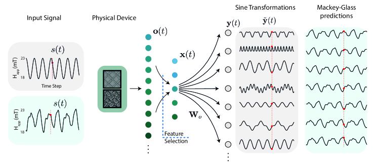
Figure 5: Schematic of offline learning. Input data is applied to the physical system producing a set of $\mathbf{o}(t)$ features. Feature selection reduces the size of $\mathbf{o}(t)$ to a new set of $\mathbf{x}(t)$ features. We then apply ridge regression to obtain a set of weights $\mathbf{W}_{o}$ to obtain the transformation / prediction $\mathbf{y}(t)$ = $\mathbf{W}_{o}$$\mathbf{x}(t)$

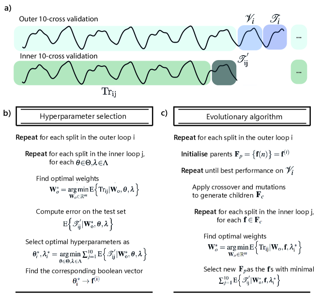
Figure 6: Scheme of the data splits for the inner and outer validation loops (a) and pseudo-codes for hyperparameter selection (b) and the evolutionary algorithm (c). The evolutionary algorithm is always applied after the hyperparameter selection (see the text for more details).

We now describe the feature selection methodology in detail. Considering the response of a system across time $\mathbf{o}(t)$, the feature selection algorithm aims to select a subset of features $\mathbf{x}(t)$ that will be used for training and evaluation. We can consider feature selection as a boolean operation over the $\mathbf{o}(t)$ feature space, where a value of one (zero) corresponds to the considered feature being used (neglected). If $m$ is the dimensionality of $\mathbf{o}(t)$, the number of possible ways to define $\mathbf{x}(t)$ is $2^{m}-1$. As a consequence, the feature selection algorithm can lead also to overfitting, therefore we must implement an appropriate methodology to define $\mathbf{x}(t)$ and to accurately measure the performance of the models.

Considering a specific split of the outer validation loop (Figure 6 a), where we select a validation set $\mathcal{V}_{i}$ and a test set $\mathcal{T}_{i}$ (comprising of the $10\%$ of the data each, i.e. 25 data points), we performed $10$ cross-validations on the remaining data to optimise hyperparameter values through grid-search. In this inner validation loop, each split corresponds to a test set $\mathcal{T}^{{}^{\prime}}_{ij}$ (comprising again of the $10\%$ of the remaining data, without $\mathcal{V}_{i}$ and $\mathcal{T}_{i}$), where changing $j$ means to select a different test-split in the inner loop based on the $i$-th original split of the outer validation (Figure 6 a). The remaining data, highlighted in green in Figure 6 a), are used for training to optimise the read-out weights and minimise the error function $\rm{E}$ through ridge-regression previously described.

At this stage, we performed a grid-search methodology on hyperparameters $\theta$ and $\lambda$ which control directly and indirectly the number of features being adopted for training (Figure 6 b). The hyperparameter $\theta$ acts as a threshold on the correlation matrix of the features. Simply, if the correlation among two features exceeds the specific value of $\theta$ considered, one of these two features is removed for training (and testing). The idea behind this method is to discard features that are highly correlated, since they would contribute in a similar way during training. This emphasises diversity in the reservoir response. The hyperparameter $\lambda$ is the penalty term in ridge-regression. Higher values of $\lambda$ lead to a stronger penalisation on the magnitude of the read-out weights. As such, $\lambda$ can help prevent overfitting and controls indirectly the number of features being adopted. We should use a high value of $\lambda$ if the model is more prone to overfitting the training dataset, a case that occurs when the number of features adopted is high. Calling $\rm{E}\Big{\{}\mathcal{T}^{{}^{\prime}}_{ij}|\mathbf{W}^{*}_{o},\theta,\lambda\Big{\}}$ the error computed on the test set $\mathcal{T}^{{}^{\prime}}_{ij}$ with weights $\mathbf{W}^{*}_{o}$ optimised on the corresponding training data ($\mathbf{W}^{*}_{o}=\operatorname*{arg\,min}\limits_{\mathbf{W}_{o}\in\mathbb{R}^{m}}\rm{E}\Big{\{}\rm{Tr}_{ij}|\mathbf{W}_{o},\theta,\lambda\Big{\}}$ in the algorithm of Figure 6 b) and with hyperparameter values $\theta$ and $\lambda$ respectively, we select the values of the hyperparameters that correspond to the minimum average error over the test sets in the inner validation loop. Otherwise stated, we select the optimal $\theta^{*}_{i}$ and $\lambda^{*}_{i}$ for the $i$-th split in the outer loop from the test average error in the inner $10$ cross-validation as $\theta^{*}_{i},\lambda^{*}_{i}=\operatorname*{arg\,min}\limits_{\theta\in\Theta,\lambda\in\Lambda}\sum_{j=1}^{10}\rm{E}\Big{\{}\mathcal{T}^{{}^{\prime}}_{ij}|\mathbf{W}^{*}_{o},\theta,\lambda\Big{\}}$. This methodology permits to find $\theta^{*}_{i}$ and $\lambda^{*}_{i}$ that are not strongly dependent on the split considered, while maintaining the parts of the dataset $\mathcal{V}_{i}$ and $\mathcal{T}_{i}$ unused during training and hyperparameter selection. The sets $\Theta$ and $\Lambda$ correspond to the values explored in the grid-search. In our case, $\Theta=\{1,0.999,0.99,0.98,0.97,...\}$ and $\Lambda=\{1e-4,1e-3,1e-2,5e-2,1e-1\}$. Repeating this procedure for each split of the outer loop, we found the optimal $\theta^{*}_{i}$ and $\lambda^{*}_{i}$, for $i=1,...,10$. This concludes the algorithm (Hyperparameter Selection) described in Figure 6 b). Selection of the hyperparameters $\theta^{*}_{i}$ permit to find subsets of features based on correlation measures. However, promoting diversity of reservoir measures does not necessarily correspond to the highest performance achievable. Thus, we adopted an evolutionary algorithm to better explore the space of possible combination of measurements (algorithm of Figure 6 c).

It is necessary now to notice how a value of $\theta^{*}_{i}$ corresponds to a $m$-dimensional boolean vector $\mathbf{f}^{(i)}$, whose $j$-th dimension is zero if its $j$-th feature $f^{(i)}_{j}$ is correlated more than $\theta^{*}_{i}$ with at least one other output. For each split $i$ in the outer loop, we adopted an evolutionary algorithm that operates over the $m$-dimensional boolean space of feature-selection, where each individual corresponds to a specific vector $\mathbf{f}$. At each evolutionary step, we performed operations of crossover and mutation over a set of $N_{p}$ parents $\mathcal{\mathbf{F}}_{p}=\big{\{}\mathbf{f}(n)\big{\}}_{n=1,...,\rm{N}_{p}}$. For each split $i$ of the outer loop and at the first evolutionary step, we initialised the parents of the algorithm to $\mathbf{f}^{(i)}$. We defined a crossover operation among two individuals $\mathbf{f}(i)$ and $\mathbf{f}(j)$ as $\mathbf{f}=\rm{CrossOver}\big{(}\mathbf{f}(i),\mathbf{f}(j)\big{)}$ where the $k$-th dimension of the new vector $\mathbf{f}$ is randomly equal to $f(i)_{k}$ or $f(j)_{k}$ with the same probability. A mutation operation of a specific $\mathbf{f}(i)$ is defined as $\mathbf{f}=\rm{Mutation}\big{(}\mathbf{f}(i)\big{)}$ by simply applying the operator $not$ to each dimension of $\mathbf{f}(i)$ with a predefined probability $p_{m}$. The application of crossovers and mutations permits the definition of a set of $\rm{N}_{c}$ children $\mathbf{F}_{c}=\big{\{}\mathbf{f}(n)\big{\}}_{n=1,...,\rm{N}_{c}}$ from which we select the $\rm{N}_{p}$ models with the highest performance over the test sets of the inner loop as parents for the next iteration. Otherwise stated, we selected the $\mathbf{F}_{p}$ vectors corresponding to the lowest values of the average error as $\mathbf{F}_{p}=\operatorname*{arg\,min^{N_{p}}}\limits_{\mathbf{f}\in\mathbf{F}_{c}}\sum_{j=1}^{10}\rm{E}\Big{\{}\mathcal{T}^{{}^{\prime}}_{ij}|\mathbf{W}^{*}_{o},\mathbf{f},\lambda^{*}_{i}\Big{\}}$ where $\operatorname*{arg\,min^{N_{p}}}$ selects the $\rm{N}_{p}$ arguments of the corresponding function with minimal values. We notice how a step of the evolutionary approach aims to minimise an error estimated in the same fashion as in the algorithm of Figure 6 b, but this time searching for the best performing set $\mathbf{F}_{p}$, rather then the best performing couple of hyperparameter values $\lambda^{*}_{i}$ and $\theta^{*}_{i}$.

Finally, we stopped the evolutionary algorithm at the iteration instance where the average performance of $\mathbf{F}_{p}$ over $\mathcal{V}_{i}$ is at minimum and selected the model $\mathbf{f}^{*}_{i}$ with the lowest error on $\mathcal{V}_{i}$. The utilisation of a separate set $\mathcal{V}_{i}$ for the stop-learning condition was necessary to avoid overfitting of the training data. Indeed, it was possible to notice how the performance on $\mathcal{V}_{i}$ would improve for the first iterations of the evolutionary algorithm and then become worse. This concludes the evolutionary algorithm depicted in Figure 6 c. At last, the overall performance of the model is computed as the sum of the mean-squared errors over the outer validation loop as $\mathcal{E}=\sum_{i=1}^{10}\rm{E}\Big{\{}\mathcal{T}_{i}|\mathbf{W}^{*}_{o},\mathbf{f}^{*}_{i},\lambda^{*}_{i}\Big{\}}$. Summarising, we can think the overall methodology as an optimisation of relevant hyperparameters followed by a fine-tuning of the set of features used through an evolutionary algorithm. The final performance and its measure of variation reported in the paper are computed as average and standard deviation over ten repetitions of the evolutionary algorithm respectively.

Meta-learning

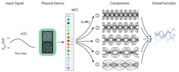
Figure 7: Schematic of the few-shot learning task. The input signal is applied to the multilayer neural network and the observations recorded. The system is then trained to learn a subset of frequency decomposition’s with minimal training data.

The goal of meta-learning is optimise an initial state for the network such that when a new task with limited data points is presented, the network can be quickly updated to give strong performance.

Let us consider a family of M tasks $\mathcal{T}=\{\mathcal{T}_{1},\mathcal{T}_{2},...,\mathcal{T}_{\rm{M}}\}$. Each task is composed by a dataset $\mathcal{D}_{i}=\Big{\{}(\mathbf{o}_{1},\tilde{\mathbf{y}}_{1}),(\mathbf{o}_{2},\tilde{\mathbf{y}}_{2}),...,(\mathbf{o}_{\rm{N}},\tilde{\mathbf{y}}_{\rm{N}})\Big{\}}$, where $\mathbf{o}$ and $\mathbf{\tilde{y}}$ correspond to observations and targets respectively (i.e. the frequency decomposition task previously described), and a cost function $\rm{E}_{\mathcal{T}_{i}}$. A meta-learning algorithm is trained on a subset of $\mathcal{T}$ and asked to quickly adapt and generalise on a new test subset of $\mathcal{T}$. Otherwise stated, the aim of meta-learning is to find an initial set of weights $\mathbf{W}(0)$ that can learn a task $\mathcal{T}_{i}$ after observing a small number of data points from $\mathcal{T}_{i}$. To achieve this, we used a variation of the MAML algorithm, which is now quickly summarised. For a given task $\mathcal{T}_{i}$, the initial set of trainable parameters $\mathbf{W}(0)$ are updated via gradient descent

$$\mathbf{W}_{i}(n)=\mathbf{W}_{i}(n-1)-\eta\nabla_{\mathbf{W}_{i}(n-1)}\rm{E}_{\mathcal{T}_{i}}$$ (1)

where $\eta$ is the learning rate. Eq.1 is repeated iteratively for $n=0,...,\tilde{n}$, where $\tilde{n}$ are the number of updates performed in each task. We notice how the subscripts $i$ on the parameters $\mathbf{W}$ are introduced because the latter become task-specific after updating, while they all start from the same values $\mathbf{W}(0)$ at the beginning of a task. MAML optimizes the parameters $\mathbf{W}(0)$ (i.e. the parameters used at the start of a task, before any gradient descent) through the minimisation of cost functions sampled from $\mathcal{T}$ and computed over the updated parameters $\mathbf{W}(n)$ i.e. the performance of a set of $\mathbf{W}(0)$ is evaluated based on the resulting $\mathbf{W}(n)$ after gradient descent. Mathematically, the aim is to find the optimal $\mathbf{W}(0)$ that minimises the meta-learning objective $\mathcal{E}$

$$\mathcal{E}=\sum_{\mathcal{T}}\rm{E}_{\mathcal{T}_{i}}(\mathcal{D}_{i}|\mathbf{W}_{i}(n))$$ (2)

Gradients of $\mathcal{E}$ need to be computed with respect to $\mathbf{W}(0)$, and this results in the optimisation of the recursive Eq. 1 and the computation of higher-order derivatives. In our case, we used the first-order approximation of the algorithm[71]. After the meta-learning process, the system is asked to learn an unseen task $\mathcal{T}_{j}$ updating $\mathbf{W}(0)$ through the iteration of Eq.1 computed on a small subset of data of $\mathcal{D}_{j}$. Strong performance is a result of quick adaptation and small MSE between the prediction and target.

In contrast to previous works, we adopted this learning framework on the response of a physical system. The optimisation occurs exclusively at the read-out level, leaving the computation of non-linear transformations and temporal dependencies to the physical network. The outcome of our application of meta-learning, depends on the richness of the dynamics of the nanomagnetic arrays. In this case, the read-out connectivity matrix is not task-specific as in previous sections, we use the same $\mathbf{W}(0)$ for different tasks.

We decompose $\mathbf{W}$ into two factors to permit rapid adaptation through one connectivity matrix. Considering the i-th output node $y_{i}$, its activity is given by $y_{i}(t)=\alpha_{i}\mathbf{w}_{i}\mathbf{o}(t)$, where $\mathbf{w}_{i}$ is the i-th row of the matrix $\mathbf{W}$ and $\alpha_{i}$ is an additional parameter. We notice how the inclusion of parameters $\alpha$s that capture the ‘magnitude’ of the weights has also been used, in a different context, for weight normalisation [83]. In the approach adopted we train the parameters $\alpha$s and $\mathbf{w}$s with different timescales of the learning process, disentangling their contribution in the inner (task-specific updates, Eq. 1) and outer loops (computation of the meta-learning objective of Eq. 2) of the MAML algorithm. Specifically, the $\alpha$s parameters are updated for each task following

$$\alpha_{i}(n)=\alpha_{i}(n-1)+\eta_{\alpha}\dfrac{\partial\rm{E}_{\mathcal{T}_{i}}}{\partial\alpha_{i}(n-1)}\ \ \rm{for}\ n=1,...,\tilde{n}$$ (3)

while the parameters $\mathbf{w}$s optimised through the meta-learning objective via

$$\mathbf{w}_{i}\leftarrow\mathbf{w}_{i}+\eta_{\mathbf{w}}\sum_{\mathcal{T}}\rm{E}_{\mathcal{T}_{j}}(\mathcal{D}_{j}|\alpha_{i}(n))$$ (4)

which is evaluated on the task-specific parameters $\alpha$s. In this way, training of the parameters $\mathbf{w}$s is accomplished after appropriate, task-dependent scaling of the output activities.

ESN Comparison

The Echo-state network of Fig. 3 b is a software model defined through

$$\mathbf{x}(t+\delta t)=(1-\alpha)\mathbf{x}(t)+\alpha f(\mathbf{W}_{in}\mathbf{s}(t)+\mathbf{W}_{esn}\mathbf{x}(t))$$ (5)

where $\mathbf{W}_{esn}$ and $\mathbf{W}_{in}$ are fixed and random connectivity matrices defined following standard methodologies [84]. In particular, the eigenvalues of the associated, linearised dynamical system are rescaled to be inside the unit circle of the imaginary plane. Training occurs on the read-out level of the system. Echo-state networks and their spiking analogous liquid-state machines [85] are the theoretical prototypes of the reservoir computing paradigm. Their performance can thus constitute an informative reference for the physically defined networks. We highlight two differences when making this comparison: first, the ESN is defined in simulations and it is consequently not affected by noise; second, the physically defined network has a feedforward topology, where the memory of the system lies in the intrinsic dynamics of each complex node and the connectivity is not random but tuned thanks to the designed methodology.
For the results of Fig.3, we varied the number of nodes of the ESN and computed the performance of the model on the task considered. For each value of the dimensionality explored, we repeated the optimization process ten times resampling the random $\mathbf{W}_{in}$ and $\mathbf{W}_{esn}$. The black dots in Fig.3 report the average performance across these repetitions as the number of nodes varies. The black line reflects a polynomial fit of such results for illustrative purposes, while the grey area reflects the dispersion of the distributions of the results.

Double gradient-descent

The section is dedicated to the details of the simulations of Fig. 1. Optimisation is accomplished through gradient-descent, in particular with the Adam optimiser[82]. We varied the dimensionality of the system to change the number of trainable parameters (x-axis). To accomplish this, a system of dimensionality n in Figure 1 is defined by selecting a subset of n features from the complete physical neural network (PNN). In this case, we selected the features following the order in which the complex nodes are introduced in the network, i.e. starting from the first layer up to the final layer of the PNN. To establish that the results are not a consequence of artefacts in the order of this selection, we reshuffled the features belonging to each layer. Every time that we increase the dimensionality of the system, new features are added to the ones previously adopted. This procedure has been performed ten times for each value of the dimensionality explored, reshuffling the data differently every time. The coloured, continuous curves reported in Figure 1 report the average performance $\langle MSE(n)\rangle$ as the dimensionality n varies, while the shadowed areas reflect the performance regions $\langle MSE(n)\rangle\pm 2\sigma_{MSE(n)}$.

Data availability statement

The datasets generated during and/or analysed during the current study are available from the corresponding author on reasonable request.

Code availability statement

The code used in this study is available from the corresponding author on reasonable request.

References

- [1] Zou, D., Cao, Y., Zhou, D. & Gu, Q. Gradient descent optimizes over-parameterized deep relu networks. \JournalTitleMachine learning 109, 467–492 (2020).
- [2] Zou, D. & Gu, Q. An improved analysis of training over-parameterized deep neural networks. \JournalTitleAdvances in neural information processing systems 32 (2019).
- [3] Marković, D., Mizrahi, A., Querlioz, D. & Grollier, J. Physics for neuromorphic computing. \JournalTitleNature Reviews Physics 2, 499–510 (2020).
- [4] Mizrahi, A. et al. Neural-like computing with populations of superparamagnetic basis functions. \JournalTitleNature communications 9, 1–11 (2018).
- [5] Gartside, J. C. et al. Reconfigurable training and reservoir computing in an artificial spin-vortex ice via spin-wave fingerprinting. \JournalTitleNature Nanotechnology 17, 460–469 (2022).
- [6] Allwood, D. A. et al. A perspective on physical reservoir computing with nanomagnetic devices. \JournalTitleApplied Physics Letters 122, 040501 (2023).
- [7] Schuman, C. D. et al. Opportunities for neuromorphic computing algorithms and applications. \JournalTitleNature Computational Science 2, 10–19 (2022).
- [8] Tanaka, G. et al. Recent advances in physical reservoir computing: A review. \JournalTitleNeural Networks 115, 100–123 (2019).
- [9] Nakajima, K. Physical reservoir computing—an introductory perspective. \JournalTitleJapanese Journal of Applied Physics 59, 060501 (2020).
- [10] Milano, G. et al. In materia reservoir computing with a fully memristive architecture based on self-organizing nanowire networks. \JournalTitleNature Materials 1–8 (2021).
- [11] Chumak, A. et al. Roadmap on spin-wave computing concepts. \JournalTitleIEEE Transactions on Quantum Engineering (2021).
- [12] Papp, Á., Porod, W. & Csaba, G. Nanoscale neural network using non-linear spin-wave interference. \JournalTitleNature communications 12, 1–8 (2021).
- [13] Cucchi, M., Abreu, S., Ciccone, G., Brunner, D. & Kleemann, H. Hands-on reservoir computing: a tutorial for practical implementation. \JournalTitleNeuromorphic Computing and Engineering (2022).
- [14] Vidamour, I. et al. Reservoir computing with emergent dynamics in a magnetic metamaterial. \JournalTitlearXiv preprint arXiv:2206.04446 (2022).
- [15] Wright, L. G. et al. Deep physical neural networks trained with backpropagation. \JournalTitleNature 601, 549–555 (2022).
- [16] Appeltant, L. et al. Information processing using a single dynamical node as complex system. \JournalTitleNature communications 2, 1–6 (2011).
- [17] Thomas, A. Memristor-based neural networks. \JournalTitleJournal of Physics D: Applied Physics 46, 093001 (2013).
- [18] Caravelli, F. & Carbajal, J. P. Memristors for the curious outsiders. \JournalTitleTechnologies 6, DOI: 10.3390/technologies6040118 (2018).
- [19] Milano, G. et al. In materia reservoir computing with a fully memristive architecture based on self-organizing nanowire networks. \JournalTitleNature Materials 21, 195–202 (2022).
- [20] Moon, J. et al. Temporal data classification and forecasting using a memristor-based reservoir computing system. \JournalTitleNature Electronics 2, 480–487 (2019).
- [21] Du, C. et al. Reservoir computing using dynamic memristors for temporal information processing. \JournalTitleNature communications 8, 1–10 (2017).
- [22] Yao, P. et al. Fully hardware-implemented memristor convolutional neural network. \JournalTitleNature 577, 641–646 (2020).
- [23] Li, C. et al. Efficient and self-adaptive in-situ learning in multilayer memristor neural networks. \JournalTitleNature communications 9, 1–8 (2018).
- [24] Sui, X., Wu, Q., Liu, J., Chen, Q. & Gu, G. A review of optical neural networks. \JournalTitleIEEE Access 8, 70773–70783 (2020).
- [25] Grollier, J. et al. Neuromorphic spintronics. \JournalTitleNature Electronics 1–11 (2020).
- [26] Torrejon, J. et al. Neuromorphic computing with nanoscale spintronic oscillators. \JournalTitleNature 547, 428–431 (2017).
- [27] Romera, M. et al. Vowel recognition with four coupled spin-torque nano-oscillators. \JournalTitleNature 563, 230–234 (2018).
- [28] Jensen, J. H., Folven, E. & Tufte, G. Computation in artificial spin ice. In Artificial Life Conference Proceedings, 15–22 (MIT Press, 2018).
- [29] Jensen, J. H. & Tufte, G. Reservoir computing in artificial spin ice. In Artificial Life Conference Proceedings, 376–383 (MIT Press, 2020).
- [30] Hon, K. et al. Numerical simulation of artificial spin ice for reservoir computing. \JournalTitleApplied Physics Express 14, 033001 (2021).
- [31] Heyderman, L. J. Spin ice devices from nanomagnets. \JournalTitleNature Nanotechnology 17, 435–436, DOI: 10.1038/s41565-022-01088-2 (2022).
- [32] Saccone, M. & et al. Direct observation of a dynamical glass transition in a nanomagnetic artificial hopfield network. \JournalTitleNature Physics 18, 517–521, DOI: 10.1038/s41567-022-01538-7 (2022).
- [33] Lee, O. et al. Task-adaptive physical reservoir computing. \JournalTitlearXiv preprint arXiv:2209.06962 (2022).
- [34] Arava, H. et al. Computational logic with square rings of nanomagnets. \JournalTitleNanotechnology 29, 265205 (2018).
- [35] Luo, Z. et al. Current-driven magnetic domain-wall logic. \JournalTitleNature 579, 214–218 (2020).
- [36] Hu, W. et al. Distinguishing artificial spin ice states using magnetoresistance effect for neuromorphic computing. \JournalTitleNature Communications 14, 2562 (2023).
- [37] Zhong, Y. et al. A memristor-based analogue reservoir computing system for real-time and power-efficient signal processing. \JournalTitleNature Electronics 5, 672–681 (2022).
- [38] Sheldon, F., Kolchinsky, A. & Caravelli, F. Computational capacity of lrc, memristive and hybrid electronic reservoirs. \JournalTitlePhys. Rev. E 106 (2022).
- [39] Stenning, K. D. et al. Magnonic bending, phase shifting and interferometry in a 2d reconfigurable nanodisk crystal. \JournalTitleACS nano (2020).
- [40] Haldar, A., Kumar, D. & Adeyeye, A. O. A reconfigurable waveguide for energy-efficient transmission and local manipulation of information in a nanomagnetic device. \JournalTitleNature nanotechnology 11, 437 (2016).
- [41] Gartside, J. C. et al. Current-controlled nanomagnetic writing for reconfigurable magnonic crystals. \JournalTitleCommunications Physics 3, 1–8 (2020).
- [42] Grundler, D. Reconfigurable magnonics heats up. \JournalTitleNature Physics 11, 438 (2015).
- [43] Chumak, A., Serga, A. & Hillebrands, B. Magnonic crystals for data processing. \JournalTitleJournal of Physics D: Applied Physics 50, 244001 (2017).
- [44] Wang, Q., Chumak, A. V. & Pirro, P. Inverse-design magnonic devices. \JournalTitleNature communications 12, 1–9 (2021).
- [45] Gartside, J. C. et al. Reconfigurable magnonic mode-hybridisation and spectral control in a bicomponent artificial spin ice. \JournalTitleNature Communications 12, 1–9 (2021).
- [46] Barman, A., Mondal, S., Sahoo, S. & De, A. Magnetization dynamics of nanoscale magnetic materials: A perspective. \JournalTitleJournal of Applied Physics 128, 170901 (2020).
- [47] Kaffash, M. T., Lendinez, S. & Jungfleisch, M. B. Nanomagnonics with artificial spin ice. \JournalTitlePhysics Letters A 402, 127364 (2021).
- [48] Barman, A. et al. The 2021 magnonics roadmap. \JournalTitleJournal of Physics: Condensed Matter (2021).
- [49] Dion, T. et al. Observation and control of collective spin-wave mode-hybridisation in chevron arrays and square, staircase and brickwork artificial spin ices. \JournalTitlearXiv preprint arXiv:2112.05354 (2021).
- [50] Arroo, D. M., Gartside, J. C. & Branford, W. R. Sculpting the spin-wave response of artificial spin ice via microstate selection. \JournalTitlePhysical Review B 100, 214425 (2019).
- [51] Dion, T. et al. Tunable magnetization dynamics in artificial spin ice via shape anisotropy modification. \JournalTitlePhysical Review B 100, 054433 (2019).
- [52] Vanstone, A. et al. Spectral-fingerprinting: Microstate readout via remanence ferromagnetic resonance in artificial spin systems. \JournalTitlearXiv preprint arXiv:2106.04406 (2021).
- [53] Chaurasiya, A. K. et al. Comparison of spin-wave modes in connected and disconnected artificial spin ice nanostructures using brillouin light scattering spectroscopy. \JournalTitleACS nano (2021).
- [54] Dambre, J., Verstraeten, D., Schrauwen, B. & Massar, S. Information processing capacity of dynamical systems. \JournalTitleScientific reports 2, 1–7 (2012).
- [55] Love, J., Mulkers, J., Bourianoff, G., Leliaert, J. & Everschor-Sitte, K. Task agnostic metrics for reservoir computing. \JournalTitlearXiv preprint arXiv:2108.01512 (2021).
- [56] Inubushi, M. & Yoshimura, K. Reservoir computing beyond memory-nonlinearity trade-off. \JournalTitleScientific reports 7, 1–10 (2017).
- [57] Goldmann, M., Köster, F., Lüdge, K. & Yanchuk, S. Deep time-delay reservoir computing: Dynamics and memory capacity. \JournalTitleChaos: An Interdisciplinary Journal of Nonlinear Science 30, 093124 (2020).
- [58] Hasson, U., Chen, J. & Honey, C. J. Hierarchical process memory: memory as an integral component of information processing. \JournalTitleTrends in cognitive sciences 19, 304–313 (2015).
- [59] Jaeger, H. Discovering multiscale dynamical features with hierarchical echo state networks. \JournalTitleDeutsche Nationalbibliothek (2007).
- [60] Manneschi, L. et al. Exploiting multiple timescales in hierarchical echo state networks. \JournalTitleFrontiers in Applied Mathematics and Statistics 6, 76 (2021).
- [61] Moon, J., Wu, Y. & Lu, W. D. Hierarchical architectures in reservoir computing systems. \JournalTitleNeuromorphic Computing and Engineering 1, 014006 (2021).
- [62] Gallicchio, C., Micheli, A. & Pedrelli, L. Deep reservoir computing: A critical experimental analysis. \JournalTitleNeurocomputing 268, 87–99 (2017).
- [63] Gallicchio, C. & Micheli, A. Echo state property of deep reservoir computing networks. \JournalTitleCognitive Computation 9, 337–350 (2017).
- [64] Gallicchio, C., Micheli, A. & Pedrelli, L. Design of deep echo state networks. \JournalTitleNeural Networks 108, 33–47 (2018).
- [65] Ma, Q., Shen, L. & Cottrell, G. W. Deepr-esn: A deep projection-encoding echo-state network. \JournalTitleInformation Sciences 511, 152–171 (2020).
- [66] Van der Sande, G., Brunner, D. & Soriano, M. C. Advances in photonic reservoir computing. \JournalTitleNanophotonics 6, 561–576 (2017).
- [67] Liang, X. et al. Rotating neurons for all-analog implementation of cyclic reservoir computing. \JournalTitleNature communications 13, 1–11 (2022).
- [68] D’Souza, R. M., di Bernardo, M. & Liu, Y.-Y. Controlling complex networks with complex nodes. \JournalTitleNature Reviews Physics 1–13 (2023).
- [69] Wang, Y., Yao, Q., Kwok, J. T. & Ni, L. M. Generalizing from a few examples: A survey on few-shot learning. \JournalTitleACM computing surveys (csur) 53, 1–34 (2020).
- [70] Vanschoren, J. Meta-learning: A survey. \JournalTitlearXiv preprint arXiv:1810.03548 (2018).
- [71] Finn, C., Abbeel, P. & Levine, S. Model-agnostic meta-learning for fast adaptation of deep networks. In International conference on machine learning, 1126–1135 (PMLR, 2017).
- [72] Mackey, M. C. & Glass, L. Oscillation and chaos in physiological control systems. \JournalTitleScience 197, 287–289 (1977).
- [73] Nakkiran, P. et al. Deep double descent: Where bigger models and more data hurt. \JournalTitleJournal of Statistical Mechanics: Theory and Experiment 2021, 124003 (2021).
- [74] Arpit, D. et al. A closer look at memorization in deep networks. In International conference on machine learning, 233–242 (PMLR, 2017).
- [75] Belkin, M., Hsu, D., Ma, S. & Mandal, S. Reconciling modern machine-learning practice and the classical bias–variance trade-off. \JournalTitleProceedings of the National Academy of Sciences 116, 15849–15854 (2019).
- [76] Skjærvø, S. H., Marrows, C. H., Stamps, R. L. & Heyderman, L. J. Advances in artificial spin ice. \JournalTitleNature Reviews Physics 2, 13–28 (2020).
- [77] Macêdo, R., Macauley, G., Nascimento, F. & Stamps, R. Apparent ferromagnetism in the pinwheel artificial spin ice. \JournalTitlePhysical Review B 98, 014437 (2018).
- [78] Li, Y. et al. Superferromagnetism and domain-wall topologies in artificial “pinwheel” spin ice. \JournalTitleACS nano 13, 2213–2222 (2018).
- [79] Manneschi, L., Lin, A. C. & Vasilaki, E. Sparce: Improved learning of reservoir computing systems through sparse representations. \JournalTitleIEEE Transactions on Neural Networks and Learning Systems (2021).
- [80] Gallicchio, C. & Micheli, A. Why layering in recurrent neural networks? a deepesn survey. In 2018 International Joint Conference on Neural Networks (IJCNN), 1–8 (IEEE, 2018).
- [81] Jaeger, H. Adaptive nonlinear system identification with echo state networks. \JournalTitleAdvances in neural information processing systems 15 (2002).
- [82] Kingma, D. P. & Ba, J. Adam: A method for stochastic optimization. \JournalTitlearXiv preprint arXiv:1412.6980 (2014).
- [83] Salimans, T. & Kingma, D. P. Weight normalization: A simple reparameterization to accelerate training of deep neural networks. \JournalTitleAdvances in neural information processing systems 29 (2016).
- [84] Lukoševičius, M. A practical guide to applying echo state networks. \JournalTitleNeural Networks: Tricks of the Trade: Second Edition 659–686 (2012).
- [85] Maass, W. Liquid state machines: motivation, theory, and applications. \JournalTitleComputability in context: computation and logic in the real world 275–296 (2011).