Zooming in on Multiquark Hadrons
within QCD Sum-Rule Approaches

Abstract

Aiming at self-consistent descriptions of multiquark hadrons (such as tetraquarks, pentaquarks, hexaquarks) by means of QCD sum rules, we note that the totality of contributions to two-point or three-point correlation functions that involve, respectively, either two or just a single operator capable of interpolating the particular multiquark under study can be straightforwardly disentangled into two disjoint classes defined by unambiguously identifiable members. The first is formed by so-called multiquark-phile contributions which indeed might support multiquarks. In the case of flavour-exotic tetraquarks, by definition composed of four (anti-) quarks of mutually different flavours, a tetraquark-phile contribution has to exhibit two or more gluon exchanges of appropriate topology. The second consists of contributions evidently not bearing any relation to multiquarks; these must be discarded when studying multiquarks by QCD sum rules. The first class only should enter the “multiquark-adequate” QCD sum rules for exotic hadrons.

1 Multiquark Hadrons, Subset of Unconventional QCD Bound States

The relativistic quantum field theory that provides the fundamental-level description of strong interactions in terms of quarks and gluons acting as fundamental degrees of freedom, quantum chromodynamics (QCD), in principle permits, as bound states of these degrees of freedom, all combinations that form a singlet under its non-Abelian gauge group SU(3). Therefore, among its bound states there have been observed not only the two categories of conventional hadrons, quark–antiquark mesons and three-quark baryons, but even (candidates for) representatives of various, likewise QCD-compatible categories of so-called nonconventional or exotic hadrons. To these belong multiquark hadrons (tetraquarks, pentaquarks, hexaquarks, heptaquarks, …), quark–gluon bound states, called hybrid, and pure-gluon bound states, (nick)named glueballs.

Within the framework of quantum field theory, the concept of QCD sum rules QSR provides a nonperturbative analytic (that is, not merely numerical) approach to bound states. QCD sum rules represent a means to comparatively easily trace back observable properties of hadrons to all the degrees of freedom and parameters entering the underlying quantum field theory, QCD. Quite generally, their derivation proceeds along a sequence of manipulations the main steps of which may be outlined by the following recipe: Identify or, if necessary, construct an operator that interpolates the hadron in your focus of interest, by having a nonvanishing matrix element if sandwiched between the vacuum and the particular hadron state, from the pool of quark and gluon field operators offered by QCD. Consider an apparently convenient correlation function of hadron interpolating operators. Evaluate the correlation function at both phenomenological hadron and fundamental QCD level. To this end: Apply the operator product expansion KGW , in order to separate perturbative from nonperturbative contributions. Allow the hadron spectrum to enter the game by inserting a complete set of hadron states. Emphasize lowest-mass hadron states by utilizing fitting Borel transformations. Assume that, above (ideally optimized ET1 ; ET2 ; ET3 ) effective thresholds, perturbative-QCD and hardly known higher-hadron contributions cancel.

Our present intention is to lift the standard QCD sum-rule formalism encoded in the above prescription – in particular, the theoretical starting point, viz., the QCD input to the correlation function – to a level better matching the group-theoretically induced peculiarities of the exotic multiquark hadrons that strikingly distinguish them from the class of ordinary hadrons ESRp ; ESRr ; TMA1 ; TMA2 ; LMS10 ; TMA3 . Specifically, for well-defined categories of tetraquarks LMS4 , we are led to suspect that this goal necessitates a QCD contribution to involve two or more gluon exchanges of suitable topology.

Below, we recall in brief some of our earlier considerations ESRp ; ESRr ; LMS10 on how to adequately optimize the QCD sum-rule approach to multiquark states. In this context, the main challenge is to identify and subsequently single out precisely those contributions to correlation functions that have the potential to influence QCD sum-rule predictions of multiquark features (Sect. 2). Upon following the route materializing thereby, anyone’s quest for increased precision should be rewarded by eventually arriving at so-called multiquark-adequate QCD sum rules (Sect. 4), as illustrated, for clarity, for the tetraquarks with “flavour-exotic” quark composition (Sect. 3). Ignoring all for the subsequent line of argument irrelevant issues (like parity or spin degrees of freedom, by notationally suppressing Dirac matrices) will enable us to focus on the essentials.

2 Tetraquark Mesons, Conceptually Simplest Form of Exotic Hadron

At present, the – at least from the experimental perspective PDG – presumably best established category of exotic multiquark hadrons seems to be formed by the totality of tetraquark mesons

$$T=[\overline{q}_{a}\,q_{b}\,\overline{q}_{c}\,q_{d}]\ ,$$ (1)

bound states of two quarks $q_{b},q_{d}$ and two antiquarks $\overline{q}_{a},\overline{q}_{c}$ carrying flavour quantum numbers

$$a,b,c,d\in\{u,d,s,c,b\}$$ (2)

and having masses $m_{a},m_{b},m_{c},m_{d}$ that (like the strong coupling) are basic parameters of QCD and will assume a prominent rôle in the tetraquark-adequate QCD sum rules drafted in Sect. 4.

Following, for the intended construction of the appropriate tetraquark-adequate QCD sum rules, the prescription recapitulated above, we first have to specify the tetraquark interpolating operators we would like to employ. Our task is significantly facilitated by the observation RLJ that, by application of suitable Fierz transformations MF , any chosen tetraquark interpolating operator may be demonstrated to be equivalent to a linear combination of merely two products

$$\theta_{\overline{a}b\overline{c}d}(x)\equiv j_{\overline{a}b}(x)\,j_{\overline{c}d}(x)\ ,\qquad\theta_{\overline{a}d\overline{c}b}(x)\equiv j_{\overline{a}d}(x)\,j_{\overline{c}b}(x)$$ (3)

of SU(3)-singlet quark–antiquark bilinear operators $j_{\overline{a}b}(x)$ interpolating conventional mesons,

$$j_{\overline{a}b}(x)\equiv\overline{q}_{a}(x)\,q_{b}(x)\ .$$ (4)

(Useful operator identities are provided by Ref. LMS111 , Eqs. (32), (36), or Ref. ESRr , Eqs. (1), (2).)

Since having in mind to unveil the deepest secrets of the tetraquark mesons by scrutinizing their effects upon contributing, by way of intermediate-state poles, to amplitudes encoding the scattering of two conventional mesons into two conventional mesons, a smart idea is to trust in correlation functions of a time-ordered product of four quark–antiquark bilinear operators (4),

$$\left\langle{\rm T}\!\left(j(y)\,j(y^{\prime})\,j^{\dagger}(x)\,j^{\dagger}(x^{\prime})\right)\right\rangle.$$ (5)

Configuration-space contractions of both pairs of quark–antiquark bilinear operators (4) yield correlation functions of two tetraquark interpolating operators (3) (cf. Subsect. 3.1.1 or 3.2.1):

$$\left\langle{\rm T}\!\left(\theta(y)\,\theta^{\dagger}(x)\right)\right\rangle=\lim_{\underset{\scriptstyle y^{\prime}\to y}{\scriptstyle x^{\prime}\to x}}\left\langle{\rm T}\!\left(j(y)\,j(y^{\prime})\,j^{\dagger}(x)\,j^{\dagger}(x^{\prime})\right)\right\rangle.$$ (6)

Configuration-space contractions of one pair of quark-bilinear operators (4) create correlation functions involving only one tetraquark interpolating operator (3) (cf. Subsect. 3.1.2 or 3.2.2):

$$\left\langle{\rm T}\!\left(j(y)\,j(y^{\prime})\,\theta^{\dagger}(x)\right)\right\rangle=\lim_{x^{\prime}\to x}\left\langle{\rm T}\!\left(j(y)\,j(y^{\prime})\,j^{\dagger}(x)\,j^{\dagger}(x^{\prime})\right)\right\rangle.$$ (7)

Now, from our point of view, at least, the decisive move towards the envisaged multiquark adequacy TMA2 of QCD sum rules is the unambiguous sorting out of all QCD-level contributions that promise to bear potential relevance for multiquarks from those that, beyond doubt, do not. Accordingly, in order to sharpen our blades, we formulated, for the case of tetraquark mesons, a simple and, in fact, rather self-evident criterion TQC1 ; TQC2 that enables us to separate the wheat from the chaff by identifying those contributions, henceforth named tetraquark-phile TQP1 ; TQP2 , that may contribute to the expected formation of some tetraquark pole: Let $p_{1},p_{2}$ and $q_{1},q_{2}$ be the four external momenta related to a generic correlation function (5). Recall the definition of the Mandelstam variable $s$ in terms of initial and final momenta $p_{1},p_{2}$ and $q_{1},q_{2}$, respectively,

$$s\equiv(p_{1}+p_{2})^{2}=(q_{1}+q_{2})^{2}\ .$$ (8)

We deem a QCD-level contribution, considered as function of $s$, tetraquark-phile if it exhibits a nonpolynomial dependence on $s$ and if it develops a branch cut that starts at the branch point

$$\hat{s}\equiv(m_{a}+m_{b}+m_{c}+m_{d})^{2}\ .$$ (9)

Whether or not the requirement of the existence of an appropriate branch point is fulfilled may easily be decided by inspection of the correlation function in question by means of the Landau equations LDL . (An illustration of their application may be found in the Appendix of Ref. ESRr .)

3 Tetraquark Mesons: Genuinely Flavour-Exotic Quark Composition

In order to keep all following applications of our notion of multiquark adequacy as transparent as possible, let us focus to the flavour-exotic tetraquarks: bound states of four (anti-) quarks of mutually different quark flavours, specified by further restriction of the characterization (2) by

$$T=[\overline{q}_{a}\,q_{b}\,\overline{q}_{c}\,q_{d}]\ ,\qquad a,b,c,d\in\{u,d,s,c,b\}\ ,\qquad a\neq b\neq c\neq d\ .$$ (10)

Resorting to our criterion of Sect. 2, we identify QCD-level contributions to the four-point correlation functions (5) maybe decisive for tetraquarks (10) by sorting out any irrelevant one. For these, the configuration-space contractions (6) and (7) provide the sought tetraquark-phile two-point and three-point correlation functions; pairing any such correlation function with the appropriate hadron-level counterpart then yields the corresponding QCD sum rule, cf. Sect. 4.

For (at least) flavour-exotic tetraquarks, the correlation functions (5) may be discriminated according to whether quark-flavour distributions of incoming and outgoing states are identical (Subsect. 3.1) or different (Subsect. 3.2); we tag the latter possibilities “flavour-preserving” or “flavour-retaining” and “flavour-rearranging” or “flavour-reordering” or the like, respectively.

3.1 Flavour-Preserving Four-Point Correlation Functions of Interpolating Currents

With respect to the complexity of the analysis, this task is definitely easier if the distribution of the quark flavours is identical in initial and final state of the four-point correlation function (5),

$$\left\langle{\rm T}\!\left(j_{\overline{a}b}(y)\,j_{\overline{c}d}(y^{\prime})\,j^{\dagger}_{\overline{a}b}(x)\,j^{\dagger}_{\overline{c}d}(x^{\prime})\right)\right\rangle,\qquad\left\langle{\rm T}\!\left(j_{\overline{a}d}(y)\,j_{\overline{c}b}(y^{\prime})\,j^{\dagger}_{\overline{a}d}(x)\,j^{\dagger}_{\overline{c}b}(x^{\prime})\right)\right\rangle.$$ (11)

3.1.1 Two-Point Correlation Functions: Two Identical Tetraquark Interpolating Operators

The analysis of the flavour-preserving case is comparatively easy ESRp : Figure 1 exemplifies the lower-order perturbative QCD-level contributions to the four-point correlation functions (11). It poses no problem to convince oneself that any tetraquark-phile among these features at least two gluon exchanges exhibiting appropriate topology, like the one depicted in Fig. 1(c). Then, as indicated by Fig. 2, the contraction (6) of a correlation function (11) decomposes into a pair of ordinary-meson QCD sum rules (Fig. 3), and a tetraquark-friendlier QCD sum rule (Fig. 4).

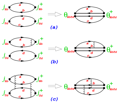
Figure 1: Flavour-preserving correlation function ESRp ; TMA2 : representative examples of contributions of the three (a,b,c) lowest perturbative orders and their contractions to two tetraquark-interpolating operators $\theta$.

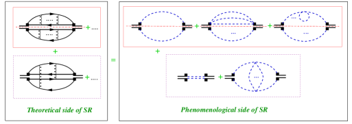
Figure 2: Flavour-preserving two-tetraquark correlation function ESRp ; TMA2 , disintegrable into (top row) two ordinary-meson QCD sum rules and (bottom row) a QCD sum rule possibly supporting tetraquark poles.

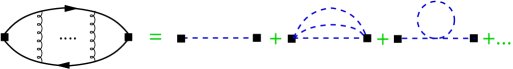
Figure 3: Conventional QCD sum rule QSR preferably applicable to ordinary mesons (blue dashed lines).

Figure 4: Refined QCD sum rule ESRp likely improving analyses of tetraquarks (blue dashed double line).

Phrased with a little bit sense of humour, the outcomes of the aforegoing discussion for the flavour-preserving partition can be subsumed by the kind of “graphical-mathematics” relation

$$\mbox{Fig.\leavevmode\nobreak\ \ref{Fsg}}=2\times(\mbox{Fig.\leavevmode\nobreak\ \ref{Fso}})+\mbox{Fig.\leavevmode\nobreak\ \ref{Fst}}\ .$$ (12)

3.1.2 Three-Point Correlation Function – One Tetraquark and Two Conventional Mesons

Given the insights established generally for the four-point correlation functions (11), identical conclusions about nature of tetraquark-phile contributions (Fig. 5), decomposition of deduced quark–hadron relations and tetraquark-fitting QCD sum rules will hold for the contraction (7).

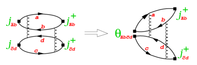
Figure 5: Flavour-retaining correlation function ESRp : typical lowest-order tetraquark-phile contribution, subject to a single contraction to a tetraquark-interpolating operator, leaving two quark-bilinear currents.

3.2 Flavour-Regrouping Four-Point Correlation Function of Interpolating Currents

Easy to guess, we now turn to the only other option for quark-flavour distribution in four-point correlation functions (5), viz., that with different flavour arrangement in initial and final states:

$$\left\langle{\rm T}\!\left(j_{\overline{a}b}(y)\,j_{\overline{c}d}(y^{\prime})\,j^{\dagger}_{\overline{a}d}(x)\,j^{\dagger}_{\overline{c}b}(x^{\prime})\right)\right\rangle.$$ (13)

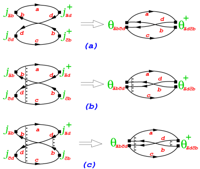
Figure 6: Flavour-redistributing correlation function ESRp ; ESRr : illustrative examples of contributions of the three (a,b,c) lowest perturbative orders and their contractions to two tetraquark-interpolating operators $\theta$.

3.2.1 Two-Point Correlation Functions: Two Different Tetraquark Interpolating Operators

In the flavour-reordering case ESRp ; ESRr , things get slightly more complicated by the fact that none of the QCD-level contributions (Fig. 6) proves to be configuration-space separable. In order to figure out which of these are tetraquark-phile, we indeed have to exploit the Landau equations LDL . These again point to the necessity of two or more gluon exchanges of adequate topology, thus opening the path for a systematics of contributions relevant or not for tetraquarks (Fig. 7).

3.2.2 Three-Point Correlation Function – One Tetraquark and Two Conventional Mesons

Due to their common origin in the four-point correlation function (5) already noted, the results gained for the two-point contraction evidently hold for the three-point contraction (Fig. 8) too.

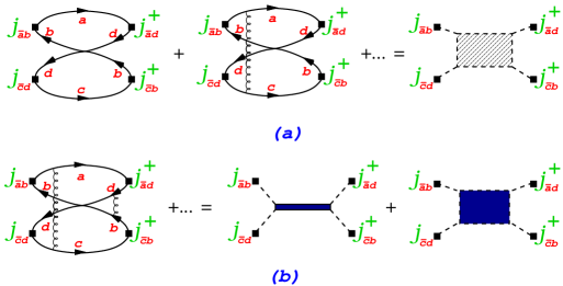
Figure 7: Flavour-reordering correlation function of four quark-bilinear operators ESRr , disintegrable into (a) an equation with no two-meson $s$-channel cut (hatched rectangle) and (b) a tetraquark-adequate QCD sum rule with two-meson $s$-channel cut (filled rectangle) and even tetraquark poles (blue horizontal bar).

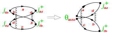
Figure 8: Flavour-rearranging correlation function ESRr : lowest-order tetraquark-phile contribution only once contracted to one tetraquark-interpolating operator, leaving two quark-bilinear currents untouched.

4 Tetraquark-Adequate QCD Sum Rules: Flavour-Exotic Tetraquarks

Application of the prescription, indicated in Sect. 1, for the extraction of a QCD sum rule from correlation functions of hadron interpolating operators entails a kind of “canonical” structure:

Evaluation of the correlation function at QCD level necessitates two sorts of contributions.

• On the one hand, there exist perturbative contributions, discriminated by the involvement of the strong coupling and usually cast in the form of a dispersion integral of a spectral density. In this integration, the assumed cancellation of higher QCD vs. higher hadron contributions is taken into account by an effective threshold $s_{\rm eff}$ which by more in-depth analysis has been revealed to depend (in a well-defined manner) on the Borel parameter $\tau$: $s_{\rm eff}=s_{\rm eff}(\tau)$ ET1 ; ET2 ; ET3 .

• On the other hand, there are nonperturbative contributions, favourably subsumed in vacuum condensates – vacuum expectation values of products of the quark and gluon field operators of QCD – which may be understood as a kind of effective parameters of QCD. Upon a Borel transformation, that is, in their Borel-transformed (or “Borelized”, for short) form, these get multiplied by powers of its Borel parameter, whence they are also called power corrections.

For the set of flavour-exotic tetraquarks, the lower-order perturbative QCD-level contributions have been analyzed in Sect. 3; an analogous – albeit somewhat more involved – discussion can be carried out, with similar results, for the nonperturbative QCD-level contributions ESRp ; ESRr ; LMS10 .

Evaluation of this correlation function at the level of the spectrum of hadron states leads to expressions that involve – in addition to the Borel parameter $\tau$ – (some of) the hadron-relevant quantities of desire. In the case of any flavour-exotic tetraquark state $|T\rangle$ specified by Eq. (10), these observables include its mass $M$, its decay constants $f$, and its vacuum–tetraquark matrix elements of a pair of quark–antiquark bilinear operators (4) in momentum space, as defined by

$$f_{\overline{a}b\overline{c}d}\equiv\langle 0|\theta_{\overline{a}b\overline{c}d}|T\rangle\ ,\qquad f_{\overline{a}d\overline{c}b}\equiv\langle 0|\theta_{\overline{a}d\overline{c}b}|T\rangle\ ,$$ (14)

$$\begin{array}[]{l}\langle 0|{\rm T}[j_{\overline{a}b}(y)\,j_{\overline{c}d}(y^{\prime})]|T\rangle\xrightarrow[\text{transformation}]{\text{Fourier}}A(T\to j_{\overline{a}b}\,j_{\overline{c}d})\ ,\\[8.61108pt] \langle 0|{\rm T}[j_{\overline{a}d}(y)\,j_{\overline{c}b}(y^{\prime})]|T\rangle\xrightarrow[\text{transformation}]{\text{Fourier}}A(T\to j_{\overline{a}d}\,j_{\overline{c}b})\ .\end{array}$$ (15)

By equating the outcomes of the above two levels of evaluation, we eventually arrive at the generic shape of multiquark-adequate QCD sum rules. It reads, for flavour-exotic tetraquarks,

$$(f_{\overline{a}b\overline{c}d})^{2}\exp(-M^{2}\,\tau) =\int_{\hat{s}}^{s_{\rm eff}(\tau)}{\rm d}s\exp(-s\,\tau)\,\rho_{\rm p}(s)+\mbox{Borelized power corrections}\ ,$$

$$f_{\overline{a}b\overline{c}d}\,A(T\to j_{\overline{a}b}\,j_{\overline{c}d})\exp(-M^{2}\,\tau) =\int_{\hat{s}}^{s_{\rm eff}(\tau)}{\rm d}s\exp(-s\,\tau)\,\Delta_{\rm p}(s)+\mbox{Borelized power corrections}\ ,$$

$$f_{\overline{a}b\overline{c}d}\,f_{\overline{a}d\overline{c}b}\exp(-M^{2}\,\tau) =\int_{\hat{s}}^{s_{\rm eff}(\tau)}{\rm d}s\exp(-s\,\tau)\,\rho_{\rm r}(s)+\mbox{Borelized power corrections}\ ,$$

$$f_{\overline{a}d\overline{c}b}\,A(T\to j_{\overline{a}b}\,j_{\overline{c}d})\exp(-M^{2}\,\tau) =\int_{\hat{s}}^{s_{\rm eff}(\tau)}{\rm d}s\exp(-s\,\tau)\,\Delta_{\rm r}(s)+\mbox{Borelized power corrections}\ ,$$

wherein the $s$-dependent functions $\rho_{\rm p,r}$ and $\Delta_{\rm p,r}$ denote, respectively, the flavour-preserving (p) and flavour-rearranging (r) spectral densities in their tetraquark-phile refinement explicated in Sect. 2, all originating in the two-point ($\rho$) and three-point ($\Delta$) correlation functions of Sect. 3.

Acknowledgements.   Both D. M. and H. S. would like to thank for support by joint CNRS/RFBR Grant PRC Russia/19-52-15022, D. M. for support by Austrian Science Fund (FWF) Project P29028-N27, and H. S. for support by EU research and innovation program Horizon 2020 under Grant Agreement 824093.

References

- (1) M.A. Shifman, A.I. Vainshtein, V.I. Zakharov, Nucl. Phys. B 147, 385 (1979)
- (2) K.G. Wilson, Phys. Rev. 179, 1499 (1969)
- (3) W. Lucha, D. Melikhov, S. Simula, Phys. Rev. D 79, 096011 (2009)
- (4) W. Lucha, D. Melikhov, S. Simula, J. Phys. G 37, 035003 (2010)
- (5) W. Lucha, D. Melikhov, S. Simula, Phys. Lett. B 687, 48 (2010)
- (6) W. Lucha, D. Melikhov, H. Sazdjian, Phys. Rev. D 100, 014010 (2019)
- (7) W. Lucha, D. Melikhov, H. Sazdjian, Phys. Rev. D 100, 074029 (2019)
- (8) W. Lucha, D. Melikhov, H. Sazdjian, PoS (EPS-HEP2019), 536 (2020)
- (9) W. Lucha, D. Melikhov, H. Sazdjian, EPJ Web Conf. 222, 03016 (2019)
- (10) W. Lucha, D. Melikhov, H. Sazdjian, Phys. Rev. D 103, 014012 (2021)
- (11) W. Lucha, D. Melikhov, H. Sazdjian, Supl. Rev. Mex. Fís. 3, 0308035 (2022)
- (12) W. Lucha, D. Melikhov, H. Sazdjian, EPJ Web Conf. 192, 00044 (2018)
- (13) R.L. Workman et al. (Particle Data Group), PTEP 2022, 083C01 (2022)
- (14) R.L. Jaffe, Nucl. Phys. A 804, 25 (2008)
- (15) M. Fierz, Z. Phys. 104, 553 (1937)
- (16) W. Lucha, D. Melikhov, H. Sazdjian, Prog. Part. Nucl. Phys. 120, 103867 (2021)
- (17) W. Lucha, D. Melikhov, H. Sazdjian, Phys. Rev. D 96, 014022 (2017)
- (18) W. Lucha, D. Melikhov, H. Sazdjian, Eur. Phys. J. C 77, 866 (2017)
- (19) W. Lucha, D. Melikhov, H. Sazdjian, PoS (EPS-HEP 2017), 390 (2018)
- (20) W. Lucha, D. Melikhov, H. Sazdjian, Phys. Rev. D 98, 094011 (2018)
- (21) L.D. Landau, Nucl. Phys. 13, 181 (1959)