Radiation-reaction and angular momentum loss at the second Post-Minkowskian order

Abstract

We compute the variation of the Fokker-Wheeler-Feynman total linear and angular momentum of a gravitationally interacting binary system under the second post-Minkowskian retarded dynamics. The resulting $O(G^{2})$ equations-of-motion-based, total change in the system’s angular momentum is found to agree with existing computations that assumed balance with angular momentum fluxes in the radiation zone.

I Introduction

The issue of angular momentum loss during the scattering of two gravitationally interacting particles has recently attracted a lot of attention Damour:2020tta ; DiVecchia:2021ndb ; Herrmann:2021lqe ; Jakobsen:2021smu ; Mougiakakos:2021ckm ; Compere:2021inq ; DiVecchia:2021bdo ; Herrmann:2021tct ; Jakobsen:2021lvp ; Bini:2021gat ; Saketh:2021sri ; Gralla:2021qaf ; Veneziano:2022zwh ; Manohar:2022dea ; Alessio:2022kwv ; DiVecchia:2022nna ; Riva:2022fru ; Kalin:2022hph ; Chen:2022fbu ; DiVecchia:2022piu ; Heissenberg:2022tsn ; Damour:2022ybd ; Porrati2022 . The existing post-Minkowskian(PM)-accurate computations of angular momentum loss have relied on an assumed balance between the angular momentum of the system of two point masses and the radiative fluxes of angular momentum at future null infinity. However, several authors have emphasized that the super-translation dependence of the definition of angular momentum at infinity raises concerns about using such balance laws for deriving effects related to the change of mechanical state of the two particles during scattering Veneziano:2022zwh ; Porrati2022 . Another puzzling feature of having an angular momentum loss at $O(G^{2})$ Damour:2020tta , while the energy-momentum loss starts at $O(G^{3})$ Herrmann:2021lqe ; Westpfahl:1987hwd , is the resulting apparent clash with the idea that, in a quantum computation, all radiative losses at infinity are a priori expected to involve the emission of real gravitons Veneziano:2022zwh .

The aim of the present work is to show that it is possible to by-pass any ambiguity concerning radiative losses of angular momentum by using an approach entirely based on the retarded equations of motion of the binary system. The possibility to do so had been first demonstrated many years ago, at the lowest Post-Newtonian (PN) order, 2.5PN, in Ref. Damour:1981bh . In the latter reference the 2PM retarded equations of motion (in harmonic coordinates) of a binary system derived in Ref. Bel:1981be were PN-expanded up to the $(v/c)^{5}$-accuracy. It was then shown that the 2PN ($(v/c)^{4}$) truncation of the equations of motion described a Poincaré-invariant conservative dynamics admitting ten Noetherian conserved quantities, namely total linear momentum and total angular momentum [23]81 .

The total variation, under the retarded dynamics, of the Noetherian linear momentum and angular momentum during scattering were then computed. This led, in particular, to a variation during scattering of the Noetherian angular momentum of the system of order $G^{2}/c^{5}$.

In the present work we extend this logic to the PM framework, without ever making use of PN expansions. More precisely, we compute the variation of the Fokker-Wheeler-Feynman Fokker:1929 ; Wheeler:1949hn total linear and angular momentum of the binary system Dettman:1954zz ; Friedman:2005rx under the exact (harmonic-coordinates) 2PM retarded dynamics Bel:1981be ; Westpfahl:1979gu . On the one hand, we find (confirming previous results Westpfahl:1987hwd ) that the variation of the total linear momentum vanishes at order $G^{2}$. On the other hand, our retarded-equations-of-motion-based computation of the total change in the Noetherian angular momentum of the system (using Lagrange’s method of variation of constants) leads to a nonzero $O(G^{2})$ result which agrees with existing computations (starting with Ref. Damour:2020tta ) that relied on computing fluxes of angular momentum at future null infinity.

We view our present study as the first step in an approach which can in principle be extended to higher PM levels. This might bring additional light on the present puzzles that affect the understanding of the 5PN dynamics Blumlein:2021txe ; Bini:2021gat ; Almeida:2022jrv . See Dlapa:2022lmu ; Bini:2022enm for a recent clarification of radiation-reaction effects at the $O(G^{4})$ level.

II Retarded force at $O(G^{2})$

We consider two gravitationally interacting point masses, $m_{1}$ and $m_{2}$, with world lines ${\mathcal{L}}_{1}$ and ${\mathcal{L}}_{2}$ having proper time parametric equations $z_{1}^{\mu}(\tau_{1})$ and $z_{2}^{\mu}(\tau_{2})$. The Poincaré-invariant retarded equations of motion of the world lines have been explicitly derived (in harmonic coordinates) at the order $G^{2}$ (second Post-Minkowskian approximation, 2PM) in Refs. Westpfahl:1979gu ; Bel:1981be . They read ($a,b=1,2$, with $a\not=b$)

$$m_{a}\frac{d^{2}z_{a}^{\mu}(\tau_{a})}{d\tau_{a}^{2}}=F_{a\rm R}^{\mu}[z_{a}(\tau_{a}),u_{a}(\tau_{a});z_{b\rm R}(\tau_{a}),u_{b\rm R}(\tau_{a})]\,,$$ (1)

where

$$F_{a\rm R}^{\mu}[z_{a},u_{a};z_{b\rm R},u_{b\rm R}]=F_{a\rm R\,,1PM}^{\mu}+F_{a\rm R\,,2PM}^{\mu}+O(G^{3})\,.$$ (2)

Here the label “R” stands for retarded, $z_{b\rm R}^{\mu}(\tau_{a})=z_{b}^{\mu}[\tau_{bR}(\tau_{a})]$ is the retarded “pre-image” of $z_{a}^{\mu}(\tau_{a})$ on ${\mathcal{L}}_{b}$,

$$(z_{a}(\tau_{a})-z_{b}[\tau_{bR}(\tau_{a})])^{2}=0\,\qquad z_{a}^{0}-z_{b\rm R}^{0}>0\,,$$ (3)

and $u_{a}^{\mu}(\tau_{a})=\frac{dz_{a}^{\mu}(\tau_{a})}{d\tau_{a}}\equiv\dot{z}_{a}$ ($a=1,2$), $u_{b\rm R}^{\mu}(\tau_{a})=u_{b}^{\mu}(\tau_{b})\big{|}_{\tau_{b}=\tau_{bR}(\tau_{a})}$.

The explicit expressions of the accelerative forces $\Gamma_{a\rm R,1PM}^{\mu}\equiv\frac{1}{m_{a}}F_{a\rm R,1PM}^{\mu}$ and $\Gamma_{a\rm R,2PM}^{\mu}\equiv\frac{1}{m_{a}}F_{a\rm R,2PM}^{\mu}$ are, for particle $m_{1}$ (see Eqs. (118)-(133) in Ref. Bel:1981be )

$$\Gamma_{1\rm R\,,1PM}^{\alpha} = \frac{Gm_{2}}{\rho_{R}^{2}}[(1-2\omega_{R}^{2})A_{R}^{\alpha}$$

$$- (1+2\omega_{R}^{2}+4A_{R}\omega_{R})v_{R}^{\alpha}]\,,$$

$$\Gamma_{1\rm R\,,2PM}^{\alpha} = \frac{G^{2}}{\rho_{R}^{3}}[m_{2}^{2}(a_{0}A_{R}^{\alpha}+c_{0}v_{R}^{\alpha})+m_{1}m_{2}(aA_{R}^{\alpha}+cv_{R}^{\alpha})]$$ (4)

$$- 4m_{1}\frac{d}{ds}[\Gamma_{1\,R}^{\alpha}\ln A_{R}]\,,$$

with

$$a_{0} = 2[2\omega_{R}^{2}+(\omega_{R}+A_{R})^{2}]\,,$$

$$c_{0} = -2[2\omega_{R}^{2}+A_{R}(\omega_{R}+A_{R})]\,,$$

$$a = -\frac{2}{A_{R}^{5}}-\frac{5\omega_{R}}{A_{R}^{4}}+\frac{5(1-2\omega_{R}^{2})}{A_{R}^{3}}+\frac{2\omega_{R}(3-4\omega_{R}^{2})}{A_{R}^{2}}$$

$$+ \frac{4(2\omega_{R}^{4}+2\omega_{R}^{2}-1)}{A_{R}}+20\omega_{R}(2\omega_{R}^{2}-1)$$

$$+ 12(2\omega_{R}^{2}-1)A_{R}\,,$$

$$c = -\frac{47}{3A_{R}^{3}}-\frac{32\omega_{R}}{A_{R}^{2}}+\frac{3+16\omega_{R}^{2}-4\omega_{R}^{4}}{A_{R}}$$

$$+ 20\omega_{R}(2\omega_{R}^{2}+3)+4(3+26\omega_{R}^{2})A_{R}+48\omega_{R}A_{R}^{2}\,.$$

Here, the various retarded scalar quantities $\rho_{R}$, $\omega_{R}$, $A_{R}$ as well as the retarded vectors $A_{R}^{\alpha}$, $v_{R}^{\alpha}$ are defined in Appendix A (in the mostly plus signature), together with their advanced counterparts . In the expression of $\Gamma_{1\rm R\,,1PM}^{\alpha}$ one has considered that the world lines were curved, and satisfied their equations of motion, at least at the required accuracy. In our present 2PM-accurate setting this means that the retarded quantities $z_{2}^{\mu}[\tau_{2R}(\tau_{1})]$ and $u_{2\rm R}^{\mu}(\tau_{1})=u_{2}^{\mu}(\tau_{2})\big{|}_{\tau_{2}=\tau_{2R}(\tau_{1})}$ entering $\Gamma_{1\rm R\,,1PM}^{\alpha}(\tau_{1})$ must be computed along world lines satisfying the 1PM equations of motion. By contrast, the evaluation of $\Gamma_{1\rm R\,,2PM}^{\alpha}$ can be done in the leading-order (LO) approximation where the curvature of the world lines is neglected.

In the (past-asymptotic) flat spacetime a basis of vectors (denoted by a bar) is naturally associated with the asymptotic incoming four-velocities of the two bodies, $\bar{u}_{1}$ and $\bar{u}_{2}$, together with two additional “initial” positions, $z_{1}^{\mu}(0),z_{2}^{\mu}(0)$, taken at $\tau_{a}=0$. The corresponding world lines have parametric equations of the form

$$z_{1}^{\mu}(\tau_{1}) = z_{1}^{\mu}(0)+\tau_{1}\bar{u}_{1}^{\mu}+\delta^{G}z_{1}^{\mu}(\tau_{1})+O(G^{2})\,,$$

$$z_{2}^{\mu}(\tau_{2}) = z_{2}^{\mu}(0)+\tau_{2}\bar{u}_{2}^{\mu}+\delta^{G}z_{2}^{\mu}(\tau_{1})+O(G^{2})\,.$$ (6)

Here $z_{a}^{\mu}(0)$ (corresponding to $\tau_{a}=0$) denotes the “midpoint” on each world line around which the magnitude of the 1PM acceleration is time-symmetric.  The $O(G)$ correction $\delta^{G}z_{a}^{\mu}(\tau_{a})$ (written below) is normalized so as to vanish at $\tau_{a}=0$. [One cannot impose the boundary condition that $\delta^{G}z_{a}^{\mu}(\tau_{a})$ vanishes at $\tau_{a}\to-\infty$ because of the logarithmic divergence of the world lines away from straight world lines in the incoming (and outgoing) states.]

The explicit expressions of the (retarded) 1PM-level terms $\delta^{G}z_{a}^{\mu}(\tau_{a})$ and $\delta^{G}u_{a}^{\mu}(\tau_{a})=\frac{d}{d\tau_{a}}\delta^{G}z_{a}^{\mu}(\tau_{a})$ read, for $a=1$ (see Eqs. (4.4) and (4.5) of Ref. Bini:2018ywr ),

$$\delta^{G}z_{1}^{\mu}(\tau_{1}) = +Gm_{2}(1-2\gamma^{2})\frac{(S(\tau_{1})-1)}{(\gamma^{2}-1)}\,\frac{b_{12}^{\mu}}{b_{0}}+Gm_{2}\frac{\gamma(2\gamma^{2}-3)}{(\gamma^{2}-1)^{3/2}}\ln\left(S(\tau_{1})\right)\,(\bar{u}_{2}^{\mu}-\gamma\bar{u}_{1}^{\mu})\,,\qquad$$

$$\delta^{G}u_{1}^{\alpha}(\tau_{1}) = +Gm_{2}\frac{(1-2\gamma^{2})S(\tau_{1})}{\sqrt{\gamma^{2}-1}D(\tau_{1})}\,\frac{b_{12}^{\mu}}{b_{0}}+Gm_{2}\frac{\gamma(2\gamma^{2}-3)}{(\gamma^{2}-1)D(\tau_{1})}(\bar{u}_{2}^{\mu}-\gamma\bar{u}_{1}^{\mu})\,,$$ (7)

with analog expressions for $a=2$ obtained by exchanging $1\leftrightarrow 2$. Here, $\gamma\equiv-\bar{u}_{1}\cdot\bar{u}_{2}$ is the Lorentz factor between the two incoming world lines and $b_{12}^{\mu}$ is a 1PM-accurate vectorial (spatial) impact parameter. More precisely, it connects the midpoints of the two world lines and its magnitude, $b_{0}$, measures the closest approach distance,

$$b_{12}^{\mu}=z_{1}^{\mu}(0)-z_{2}^{\mu}(0)\,\,;\,\,b_{0}=|b_{12}^{\mu}|=|z_{1}^{\mu}(0)-z_{2}^{\mu}(0)|\,.$$ (8)

The vectorial impact parameter $b_{12}^{\mu}$ has been chosen to be orthogonal to the two incoming four velocities $\bar{u}_{1}$ and $\bar{u}_{2}$. The auxiliary functions $S(\tau)$ and $D(\tau)$ entering Eq. (II) are defined as follows

$$D(\tau) = \sqrt{b_{0}^{2}+\tau^{2}(\gamma^{2}-1)}\,,$$

$$S(\tau) = \frac{1}{b_{0}}\left(\tau\sqrt{\gamma^{2}-1}+D(\tau)\right)\,,$$ (9)

so that $D(0)=b_{0}$ and $S(0)=1$, thereby ensuring that $\delta^{G}z_{a}^{\mu}(\tau_{a}=0)=0$. [By contrast, $\delta^{G}u_{a}^{\alpha}(\tau_{1})$ does not vanish at $\tau_{a}=0$ but vanishes at $\tau_{a}\to-\infty$ because of our chosen boundary conditions.] In addition, we have the identity $S(\tau)S(-\tau)=1$.

When working in the (incoming) rest frame of particle 1, $e_{0}^{\mu}=\bar{u}_{1}^{\mu}$, as we shall often do below, it is convenient to introduce two spatial unit vectors

$$e_{x}^{\mu} = \hat{b}_{12}^{\mu}=\frac{b_{12}^{\mu}}{b_{0}}\,,$$

$$e_{y}^{\mu} = -\frac{\bar{u}_{2}^{\mu}-\gamma\bar{u}_{1}^{\mu}}{\sqrt{\gamma^{2}-1}}\,.$$ (10)

Note that $e_{y}$ is linked to the projection of $\bar{u}_{2}$ orthogonally to $u_{1}$ in the following way

$$v = P(\bar{u}_{1})\bar{u}_{2}\equiv\bar{u}_{2\perp 1}=\bar{u}_{2}-\gamma\bar{u}_{1}$$ (11)

$$= -\sqrt{\gamma^{2}-1}e_{y}\,,$$

with the projector $P(u)$ orthogonal to the timelike direction $u$ ($u\cdot u=-1$) defined as

$$P(u)^{\mu}{}_{\nu}=\delta^{\mu}{}_{\nu}+u^{\mu}u_{\nu}\,.$$ (12)

The third spatial vector ${\bf e}_{z}={\bf e}_{x}\times{\bf e}_{y}$ does not enter the parametrization of the two world lines because the motion takes place in the $x$-$y$ plane. The minus sign in the definition of $e_{y}^{\mu}$ has been chosen so that the center-of-mass (c.m.) angular momentum is aligned with the $z$-axis: $J^{xy}_{\rm c.m.}=J^{z}_{\rm c.m.}>0$. At the 1PM approximation the magnitude of the c.m. angular momentum is (see Appendix D of Ref. Bini:2018ywr )

$$J_{\rm c.m.}=b\,P_{\rm c.m.}\,,$$ (13)

where $P_{\rm c.m.}$ is the common magnitude of the two incoming spatial linear momenta in the c.m. frame, and where the (incoming) impact parameter $b_{\rm in}$ is given by

$$b_{\rm in}=b_{0}+G(m_{1}+m_{2})\frac{(2\gamma^{2}-1)}{\gamma^{2}-1}+O(G^{2})\,.$$ (14)

Note that $b_{\rm in}$ differs from the minimal approaching distance $b_{0}=|b_{12}^{\mu}|=|z_{1}^{\mu}(0)-z_{2}^{\mu}(0)|$ by terms of order $G$.

In the incoming rest frame of particle 1 defined above the explicit expressions of the incoming four velocities read

$$\bar{u}_{1}^{\mu} = \delta_{0}^{\mu}\,,\qquad\bar{u}_{2}^{\mu}=\gamma\delta_{0}^{\mu}-\sqrt{\gamma^{2}-1}\delta_{y}^{\mu}\,,$$ (15)

while the explicit expressions of the two world lines read (if one takes $z_{1}^{\mu}(0)$ and $z_{2}^{\mu}(0)$ in the form $z_{a}^{\mu}(0)=b_{a}e_{x}^{\mu}$)

$$z_{1}^{\alpha}(\tau_{1}) = b_{1}e^{\alpha}_{x}+\bar{u}_{1}^{\alpha}\tau_{1}+Gm_{2}(1-2\gamma^{2})\frac{(S(\tau_{1})-1)}{(\gamma^{2}-1)}\,e^{\alpha}_{x}-Gm_{2}\frac{\gamma(2\gamma^{2}-3)}{\gamma^{2}-1}\ln\left(S(\tau_{1})\right)\,e^{\alpha}_{y}\,,$$

$$u_{1}^{\alpha}(\tau_{1}) = \bar{u}_{1}^{\alpha}+Gm_{2}\frac{(1-2\gamma^{2})S(\tau_{1})}{\sqrt{\gamma^{2}-1}D(\tau_{1})}\,e^{\alpha}_{x}-Gm_{2}\frac{\gamma(2\gamma^{2}-3)}{\sqrt{\gamma^{2}-1}D(\tau_{1})}e^{\alpha}_{y}\,,$$

$$z_{2}^{\alpha}(\tau_{2}) = b_{2}e^{\alpha}_{x}+\bar{u}_{2}^{\alpha}\tau_{2}-Gm_{1}(1-2\gamma^{2})\frac{(S(\tau_{2})-1)}{(\gamma^{2}-1)}\,e^{\alpha}_{x}+Gm_{1}\frac{\gamma(2\gamma^{2}-3)}{(\gamma^{2}-1)^{3/2}}\ln\left(S(\tau_{2})\right)\,v^{\prime}{}^{\alpha}$$

$$u_{2}^{\alpha}(\tau_{2}) = \bar{u}_{2}^{\alpha}-Gm_{1}\frac{(1-2\gamma^{2})S(\tau_{2})}{\sqrt{\gamma^{2}-1}D(\tau_{2})}\,e^{\alpha}_{x}+Gm_{1}\frac{\gamma(2\gamma^{2}-3)}{(\gamma^{2}-1)D(\tau_{2})}v^{\prime}{}^{\alpha}\,.$$ (16)

When performing explicit calculations it is useful to choose $b_{1}=b_{0}>0$ and $b_{2}=0$. Here, we have used the notation (see Ref. Bini:2021gat , Eq. (3.46) there)

$$v^{\prime} = P(\bar{u}_{2})\bar{u}_{1}\equiv\bar{u}_{1\perp 2}=\bar{u}_{1}-\gamma\bar{u}_{2}$$ (17)

$$= -(\gamma^{2}-1)e_{0}+\gamma\sqrt{\gamma^{2}-1}e_{y}\,.$$

Inserting in $\Gamma_{a\rm R\,,1PM}^{\alpha}$ the explicit expressions of the 1PM-accurate world lines (as functions of $\tau_{a}$) re-defines $F_{a\rm R}^{\mu}$ as a function of $\tau_{a}$ (rather than as a functional of the world lines) that we will denote as ${\mathcal{F}}_{a\rm R}^{\mu}(\tau_{a})$ to distinguish it from the original world line-dependent force, Eq. (2). Expanding ${\mathcal{F}}_{a\rm R}^{\mu}(\tau_{a})$ in powers of $G$ then yields

$${\mathcal{F}}_{a\rm R}^{\mu}(\tau_{a})={\mathcal{F}}_{a\rm R}^{G\,\mu}(\tau_{a})+{\mathcal{F}}_{a\rm R}^{G^{2}\,\mu}(\tau_{a})+O(G^{3})\,.$$ (18)

The 1PM expression of the force, ${\mathcal{F}}_{a\rm R}^{G\,\mu}(\tau_{a})$, is obtained by inserting the LO straight line world lines, namely

$$\bar{z}_{a}(\tau_{a})=z_{a}(0)+\bar{u}_{a}\tau_{a}\,,$$ (19)

in $F_{a\rm R\,,1PM}^{\mu}$ and explicitly reads

$${\mathcal{F}}_{a\rm R}^{G\,\mu}(\tau_{a}) = \frac{Gm_{a}m_{b}}{|\bar{z}_{a}(\tau_{a})-\bar{z}_{b\perp}(\tau_{a})|^{3}}\left[4(\gamma^{2}-1)b_{ab}^{\mu}\right.$$

$$\left.-(2\gamma^{2}-3)(\delta^{\mu}_{\nu}+\bar{u}_{a}^{\mu}\bar{u}_{a\nu})(\bar{z}_{a}^{\nu}(\tau_{a})-\bar{z}_{b\perp}^{\nu}(\tau_{a}))\right]\,,$$

where $a=1,2$, $b\not=a$, $b_{ab}^{\mu}=z_{a}^{\mu}(0)-z_{b}^{\mu}(0)$, and $\bar{z}_{b\perp}^{\nu}(\tau_{a})$ is the foot of the perpendicular of the point $\bar{z}_{a}^{\nu}(\tau_{a})$ on the (straight) line ${\mathcal{L}}_{b}$, so that

$$\bar{z}_{a}^{\nu}(\tau_{a})-\bar{z}_{b\perp}^{\nu}(\tau_{a}) = \bar{z}_{a}^{\nu}(\tau_{a})-z_{b}^{\nu}(0)$$ (21)

$$+ [\bar{u}_{b}\cdot(\bar{z}_{a}(\tau_{a})-z_{b}(0)]\bar{u}_{b}^{\nu}\,.\qquad$$

Explicitly, for $a=1$, we have $|\bar{z}_{1}(\tau_{1})-\bar{z}_{2\perp}(\tau_{1})|=D(\tau_{1})$ and

$${\mathcal{F}}_{1\rm R}^{G\,\mu}(\tau_{1}) = \frac{Gm_{1}m_{2}}{D(\tau_{1})^{3}}\left[(1-2\gamma^{2})b_{12}^{\mu}\right.$$ (22)

$$\left.+\tau_{1}(2\gamma^{2}-3)\gamma(\gamma\bar{u}_{1}^{\mu}-\bar{u}_{2}^{\mu})\right]\,.$$

By contrast, ${\mathcal{F}}_{a\rm R}^{G^{2}\,\mu}(\tau_{a})$ is obtained as the sum of two contributions, one coming from inserting in $F_{a\rm R\,,1PM}^{\mu}$ the $O(G)$-corrected world lines, Eq. (II), and the other one coming directly from $F_{a\rm R\,,2PM}^{\mu}$. We will not need here the (complicated) explicit expression of the retarded second-order force ${\mathcal{F}}_{a\rm R}^{G^{2}\,\mu}$, but only of its time-odd part, see below.

III Retarded vs advanced force at $O(G^{2})$

In the previous section we considered the physical, retarded equations of motions of two gravitationally interacting point masses. In order to decompose this retarded dynamics in a conservative part and a dissipative part it is useful, in our present PM framework, to consider the advanced counterpart of the equations of motion.

Introducing an indicator $\epsilon$, with $\epsilon=1$ in the retarded case and $\epsilon=-1$ in the advanced one, the generalized equations of motion are obtained as follows.

The generalized form (valid for $\epsilon=\pm 1$) of the world-line-functional version of the equations of motion reads

$$m_{a}\frac{d^{2}z_{a}^{\mu}(\tau_{a})}{d\tau_{a}^{2}}=F_{a\epsilon}^{\mu}[z_{a}(\tau_{a}),u_{a}(\tau_{a});z_{b\epsilon}(\tau_{a}),u_{b\epsilon}(\tau_{a})]\,.$$ (23)

This then yields the corresponding $\tau_{a}$-dependent generalized forces

$${\mathcal{F}}_{a\epsilon}^{\mu}(\tau_{a})={\mathcal{F}}_{a\epsilon}^{G\,\mu}(\tau_{a})+{\mathcal{F}}_{a\epsilon}^{G^{2}\,\mu}(\tau_{a})+O(G^{3})\,.$$ (24)

As is evident from Eqs. (II)-(22), the $O(G)$ force in this equation, ${\mathcal{F}}_{a\epsilon}^{G\,\mu}(\tau_{a})$, is time-symmetric, and does not depend on $\epsilon$ (we henceforth denote it with a label “$0$” in place of $\epsilon$),

$${\mathcal{F}}_{a\epsilon}^{G\,\mu}(\tau_{a})={\mathcal{F}}_{a0}^{G\,\mu}(\tau_{a})\,.$$ (25)

The time-asymmetry in the $\tau_{a}$-dependent version of the equations of motion only enters at order $G^{2}$, as is discussed in detail below.

The $\epsilon$-dependent world line equations of motion read

$$\frac{du_{a\epsilon}^{\alpha}}{d\tau_{a}}=\Gamma_{a\,\epsilon,\rm 1PM}^{\alpha}(\tau_{a})+\Gamma_{a\,\epsilon,\rm 2PM}^{\alpha}(\tau_{a})+O(G^{3})\,.$$ (26)

For $a=1$, one has

$$\Gamma_{1\,\epsilon,\rm 1PM}^{\alpha} = \frac{Gm_{2}}{\rho_{\epsilon}^{2}}[(1-2\omega_{\epsilon}^{2})A_{\epsilon}^{\alpha}$$

$$- \epsilon(1+2\omega_{\epsilon}^{2}+4A_{\epsilon}\omega_{\epsilon})v_{\epsilon}^{\alpha}]\,,$$

$$\Gamma_{1\,\epsilon,\rm 2PM}^{\alpha} = \frac{G^{2}}{\rho_{\epsilon}^{3}}[m_{2}^{2}(a_{0}A_{\epsilon}^{\alpha}+\epsilon c_{0}v_{\epsilon}^{\alpha})$$ (27)

$$+ m_{1}m_{2}(aA_{\epsilon}^{\alpha}+c\epsilon v_{\epsilon}^{\alpha})]$$

$$- 4m_{1}\epsilon\frac{d}{d\tau_{1}}[\Gamma_{1\,\epsilon 1PM}^{\alpha}\ln A_{\epsilon}]\,.$$

The explicit expressions of the $\epsilon$-dependent quantities entering these equations are defined in Appendix A. [The formal expression of the coefficients $a_{0},c_{0}$ and $a,c$ are obtained from those listed above in Eqs. (II) by replacing $R$ by $\epsilon$.] Let us also display the following intermediate results (where $\delta\equiv\delta^{G}$ and $O(G^{2})$ error terms are implicit)

$$\tau_{2\epsilon}(\tau_{1}) = \gamma\tau_{1}-\epsilon D(\tau_{1})+\delta\tau_{2\epsilon}(\tau_{1})\,,$$

$$\rho_{\epsilon}(\tau_{1}) = D(\tau_{1})+\delta\rho_{\epsilon}(\tau_{1})\,,$$

$$\omega_{\epsilon}(\tau_{1}) = -\gamma+\delta\omega_{\epsilon}(\tau_{1})\,,$$

$$A_{\epsilon}(\tau_{1}) = \gamma-\epsilon\frac{\gamma^{2}-1}{D(\tau_{1})}\tau_{1}+\delta A_{\epsilon}(\tau_{1})\,,$$

$$A^{\mu}_{\epsilon}(\tau_{1}) = \frac{1}{D(\tau_{1})}\left[b_{0}e_{x}^{\mu}+\sqrt{\gamma^{2}-1}(\gamma\tau_{1}-\epsilon D(\tau_{1}))e_{y}^{\mu}\right]$$

$$+ \delta A^{\mu}_{\epsilon}(\tau_{1})\,,$$

$$v^{\mu}_{\epsilon}(\tau_{1}) = -\sqrt{\gamma^{2}-1}e_{y}^{\mu}+\delta v^{\mu}_{\epsilon}(\tau_{1})\,,$$ (28)

with $O(G)$-corrections given by

$$\delta\tau_{2\epsilon}(\tau_{1}) = \frac{1}{D}\left[\frac{\sqrt{\gamma^{2}-1}}{\gamma}\epsilon\tau_{1}\delta z_{2}^{y}(\tau_{2\epsilon}(\tau_{1}))\right.$$

$$- \epsilon\sqrt{\gamma^{2}-1}(\gamma\tau_{1}-\epsilon D(\tau_{1}))\delta z_{1}^{y}(\tau_{1})$$

$$+ \left.\epsilon b_{0}\delta z_{2}^{x}(\tau_{2\epsilon}(\tau_{1}))-\epsilon b_{0}\delta z_{1}^{x}(\tau_{1})\right]\,,$$

$$\delta\omega_{\epsilon}(\tau_{1}) = \frac{\sqrt{\gamma^{2}-1}}{\gamma}\delta u_{2}^{y}(\tau_{2\epsilon}(\tau_{1}))-\delta u_{1}^{y}(\tau_{1})\sqrt{\gamma^{2}-1}\,,$$

$$\delta\rho_{\epsilon}(\tau_{1}) = -\epsilon b_{0}\delta u_{2}^{x}(\tau_{2\epsilon}(\tau_{1}))-\epsilon\frac{\sqrt{\gamma^{2}-1}}{\gamma}\tau_{1}\delta u_{2}^{y}(\tau_{2\epsilon}(\tau_{1}))$$

$$- \frac{b_{0}}{D(\tau_{1})}\delta z_{2}^{x}(\tau_{2\epsilon}(\tau_{1}))+\frac{b_{0}}{D(\tau_{1})}\delta z_{1}^{x}(\tau_{1})$$

$$- \tau_{1}\frac{\sqrt{\gamma^{2}-1}}{\gamma D(\tau_{1})}\delta z_{2}^{y}(\tau_{2\epsilon}(\tau_{1}))$$

$$+ \frac{\gamma}{D(\tau_{1})}\sqrt{\gamma^{2}-1}\tau_{1}\delta z_{1}^{y}(\tau_{1})\,,$$

$$\delta v^{\mu}_{\epsilon}(\tau_{1}) = -\delta u_{1}^{y}(\tau_{1})\sqrt{\gamma^{2}-1}e_{0}^{\mu}$$ (29)

$$+ \left(\delta u_{2}^{x}(\tau_{2\epsilon}(\tau_{1}))-\delta u_{1}^{x}(\tau_{1})\gamma\right)e_{x}^{\mu}$$

$$+ \left(\delta u_{2}^{y}(\tau_{2\epsilon}(\tau_{1}))-\delta u_{1}^{y}(\tau_{1})\gamma\right)e_{y}^{\mu}\,,$$

and similarly for $\delta A^{\mu}_{\epsilon}(\tau_{1})$ and $\delta A_{\epsilon}(\tau_{1}$), not shown here because involving longer expressions. All quantities here are supposed to be functions of $\tau_{1}$. In view of Eq. (25), the 1PM-accurate solutions of the $\epsilon$-dependent equations of motion, Eqs. (III), coincide with the retarded solution displayed [as functional of $\bar{u}_{a}$ and $z_{a}(0)$] in Eq.(II) above,

$$z_{a\epsilon}^{\alpha}(\tau_{a}) = z_{aR}^{\alpha}(\tau_{a})+O(G^{2})\,,$$

$$u_{a\epsilon}^{\alpha}(\tau_{a}) = u_{aR}^{\alpha}(\tau_{a})+O(G^{2})\,.$$ (30)

IV Time-symmetric dynamics at $O(G^{2})$

Our aim here is to decompose the retarded two-body dynamics in conservative and dissipative parts. To do this in a PM framework, one can first define a time-symmetric version of the 2PM dynamics by solving Einstein’s equations from the start with a time-symmetric Green’s function in 4 dimensions,

$$G_{\mu\nu\alpha\beta}^{\rm S}(x,y)=P_{\mu\nu\alpha\beta}\delta((x-y)^{2})\,,$$ (31)

where $P_{\mu\nu\alpha\beta}=\eta_{\mu\alpha}\eta_{\nu\beta}-\frac{1}{2}\eta_{\mu\nu}\eta_{\alpha\beta}$. It can be easily checked that, at order $G^{2}$ included, the use of such a time-symmetric propagator leads to equations of motion involving the following time-symmetric forces

$$F_{aS}^{\mu}[z_{a},u_{a},z_{bR},u_{bR},z_{bA},u_{bA}] = \frac{1}{2}(F_{aR}^{\mu}+F_{aA}^{\mu})$$ (32)

$$+ O(G^{3})\,,$$

with corresponding $\tau_{a}$-dependent forces

$${\mathcal{F}}_{aS}^{\mu}(\tau_{a}) = {\mathcal{F}}_{a0}^{G\,\mu}(\tau_{a})+\frac{1}{2}({\mathcal{F}}_{a\rm R}^{G^{2}\,\mu}(\tau_{a})+{\mathcal{F}}_{a\rm A}^{G^{2}\,\mu}(\tau_{a}))$$ (33)

$$+ O(G^{3})\,.$$

When using the time-symmetric Green’s function, the dynamics can be derived from a Fokker(-Wheeler-Feynman) action Fokker:1929 ; Wheeler:1949hn ; Friedman:2005rx of the general form

$$I = -\sum_{a}m_{a}\int d\tau_{a}(-\dot{z}_{a\mu}\dot{z}_{a}^{\mu})^{1/2}$$ (34)

$$+ \sum_{a<b}\iint d\tau_{a}d\tau_{b}\Lambda_{ab}+\sum_{a<b<c}\iiint d\tau_{a}d\tau_{b}d\tau_{c}\Lambda_{abc}$$

$$+ O(G^{3})\,,$$

where the one-graviton exchange ($O(G)$) contribution explicitly reads (see Eq. (22) of Ref. Friedman:2005rx )

$$\Lambda_{ab}(z_{a}-z_{b},\dot{z}_{a},\dot{z}_{b})=2Gm_{a}m_{b}\delta[(z_{a}-z_{b})^{2}]\times\qquad\qquad$$

$$\qquad\frac{(\dot{z}_{a}\cdot\dot{z}_{b})^{2}-\frac{1}{2}(\dot{z}_{a}\cdot\dot{z}_{a})(\dot{z}_{b}\cdot\dot{z}_{b})}{(-\dot{z}_{a}\cdot\dot{z}_{a})^{1/2}(-\dot{z}_{b}\cdot\dot{z}_{b})^{1/2}}\,,\qquad$$

$$\qquad=2Gm_{a}m_{b}\delta[(z_{a}-z_{b})^{2}]P_{\mu\nu\alpha\beta}u_{a}^{\mu}u_{a}^{\nu}u_{b}^{\alpha}u_{b}^{\beta}\,,$$ (35)

and where $\Lambda_{abc}$ refers to the one-loop, order $G^{2}$, interaction, etc.

The existence of such a Poincaré-invariant Fokker action guarantees that the corresponding time-symmetric dynamics has all the Noetherian conserved quantities associated with the Poincaré symmetries, namely total linear momentum and total angular momentum of the system Wheeler:1949hn ; Dettman:1954zz ; Friedman:2005rx

$$P_{\mu}^{\rm sys}(\tau_{1},\tau_{2}) = P_{\mu}^{\rm kin}(\tau_{1},\tau_{2})+P_{\mu}^{\rm int}(\tau_{1},\tau_{2})\,,$$

$$J_{\mu\nu}^{\rm sys}(\tau_{1},\tau_{2}) = J_{\mu\nu}^{\rm kin}(\tau_{1},\tau_{2})+J_{\mu\nu}^{\rm int}(\tau_{1},\tau_{2})\,.$$ (36)

The conserved quantities of the system are obtained as the sum of kinematical contributions ($P_{\mu}^{\rm kin}(\tau_{1},\tau_{2})$, $J_{\mu\nu}^{\rm kin}(\tau_{1},\tau_{2})$) and (field-mediated) interaction ones ($P_{\mu}^{\rm int}(\tau_{1},\tau_{2})$, $J_{\mu\nu}^{\rm int}(\tau_{1},\tau_{2})$). The kinematical contributions read

$$P_{\mu}^{\rm kin}(\tau_{1},\tau_{2}) = \sum_{a}m_{a}u_{a\mu}(\tau_{a})\,,$$

$$J_{\mu\nu}^{\rm kin}(\tau_{1},\tau_{2}) = \sum_{a}m_{a}(z_{a}(\tau_{a})\wedge u_{a}(\tau_{a}))_{\mu\nu}\,,$$ (37)

where the wedge product symbol is defined as

$$(A\wedge B)^{\mu\nu}\equiv A^{\mu}B^{\nu}-A^{\nu}B^{\mu}\equiv A^{\mu}\wedge B^{\nu}\,.$$ (38)

The “interaction” or “Fokker” parts of the linear momentum and of the angular momentum read, at the one-graviton exchange level,

$$P^{\rm int}_{\alpha}(\tau_{1},\tau_{2}) = \int_{-\infty}^{\infty}d\bar{\tau}\frac{\partial\Lambda}{\partial\dot{z}_{1}^{\alpha}}(\tau_{1},\bar{\tau})+\int_{-\infty}^{\infty}d\tau\frac{\partial\Lambda}{\partial\dot{z}_{2}^{\alpha}}(\tau,\tau_{2})$$

$$+ 2\left(\int_{\tau_{1}}^{\infty}\int_{-\infty}^{\tau_{2}}-\int_{-\infty}^{\tau_{1}}\int_{\tau_{2}}^{\infty}\right)d\tau d\bar{\tau}\times$$

$$(z_{1}(\tau)-z_{2}(\bar{\tau}))_{\alpha}\frac{\partial\Lambda}{\partial w}\,,$$

$$J_{\mu\nu}^{\rm int}(\tau_{1},\tau_{2}) = \int_{-\infty}^{\infty}d\bar{\tau}[(z_{1}\wedge{\mathcal{P}}_{1})(\tau_{1},\bar{\tau})]_{\mu\nu}$$ (39)

$$+ \int_{-\infty}^{\infty}d\tau[(z_{2}\wedge{\mathcal{P}}_{2})(\tau,\tau_{2})]_{\mu\nu}$$

$$+ \left(\int_{\tau_{1}}^{\infty}\int_{-\infty}^{\tau_{2}}-\int_{-\infty}^{\tau_{1}}\int_{\tau_{2}}^{\infty}\right)\left[(z_{1}\wedge{\mathcal{Q}})(\tau,\bar{\tau})\right.$$

$$+ \left.(\dot{z}_{1}\wedge{\mathcal{P}}_{1})(\tau,\bar{\tau})\right]_{\mu\nu}d\tau d\bar{\tau}\,.$$

Considering $\Lambda=\Lambda_{12}$ (see Eq. (IV) above) as a function of

$$w\equiv R_{\beta}R^{\beta}=(z_{1}-z_{2})^{2}\,,\quad R_{\beta}=(z_{1}-z_{2})_{\beta}\,,$$ (40)

as well as of $\dot{z}_{1}^{\mu}$, $\dot{z}_{2}^{\mu}$, $\Lambda=\Lambda(w,\dot{z}_{1}^{\mu},\dot{z}_{2}^{\mu})$, the values of the quantities entering the interaction terms are

$${\mathcal{P}}_{1\beta} = \frac{\partial\Lambda}{\partial\dot{z}_{1}^{\beta}}\,,$$

$${\mathcal{P}}_{2\beta} = \frac{\partial\Lambda}{\partial\dot{z_{2}}{}^{\beta}}\,,$$

$${\mathcal{Q}}_{\beta} = \frac{\partial\Lambda}{\partial R^{\beta}}=2(z_{1}-z_{2})_{\beta}\frac{\partial\Lambda}{\partial w}\,.$$ (41)

At order $G$ the interaction terms only depend on two finite segments on the world lines. This fact means, in particular, that there are no logarithmic divergences (and related logarithmic ambiguities) in the definition of $J^{\mu\nu}_{\rm sys}$.

The conservation of the system Noetherian quantities means their independence on $\tau_{1}$ and $\tau_{2}$. In the present work we will not need the explicit expressions of the total Noetherian quantities at order $G^{2}$. What is important for us is only the fact that they exist for the time-symmetric dynamics. We will, however, present an explicit computation of the Noetherian quantities at the 1PM accuracy in order to see the importance of the presence of interaction terms to ensure the conservation of manifestly Poincaré-invariant total linear momentum and angular momentum.

We will explicitly compute below at order $G$ the Noetherian quantities $P_{\mu}^{\rm sys}$ and $J_{\mu\nu}^{\rm sys}$ and show their conservation. The existence of interaction contributions (starting at the $O(G)$ level) to both linear momentum and angular moment is well-known in the PN context. For instance, at the 1PN level (see Ref. [23]81 for the 2PN case), the Poincaré-invariance of the (harmonic coordinates) Lorentz-Droste-Einstein-Infeld-Hoffmann Lagrangian yields both a conserved 1PN-accurate linear momentum $P^{\mu}=((m_{1}+m_{2})c^{2}+E,P^{i})$ and a 1PN-accurate angular momentum $J^{\mu\nu}$. Explicitly (with $v_{a}^{i}=dz_{a}^{i}/dt$)

$$E = \frac{1}{2}m_{1}v_{1}^{2}-\frac{Gm_{1}m_{2}}{2r_{12}}+\frac{1}{c^{2}}\left[\frac{3}{8}m_{1}v_{1}^{4}\right.$$ (42)

$$+ \frac{Gm_{1}m_{2}}{r_{12}}\left(-\frac{1}{4}(n_{12}v_{1})(n_{12}v_{2})+\frac{3}{2}v_{1}^{2}-\frac{7}{4}(v_{1}v_{2})\right)$$

$$+ \left.\frac{G^{2}m_{1}^{2}m_{2}}{2r_{12}^{2}}\right]+1\leftrightarrow 2\,,$$

and

$$P^{i}=p_{1}^{i}+p_{2}^{i}\,,$$ (43)

where

$${\mathbf{p}}_{1} = m_{1}{\mathbf{v}}_{1}+\frac{1}{c^{2}}\left[\frac{1}{2}m_{1}v_{1}^{2}{\mathbf{v}}_{1}\right.$$

$$+ \left.\frac{Gm_{1}m_{2}}{r_{12}}\left(-\frac{1}{2}(n_{12}v_{2}){\mathbf{n}}_{12}+3{\mathbf{v}}_{1}-\frac{7}{2}{\mathbf{v}}_{2}\right)\right]$$

with ${\mathbf{p}}_{2}$ obtained by exchanging $1\leftrightarrow 2$.

The spatial components of the angular momentum $J_{ij}=\epsilon_{ijk}J_{k}$ are

$${\mathbf{J}} = {\mathbf{z}}_{1}\times{\mathbf{p}}_{1}+{\mathbf{z}}_{2}\times{\mathbf{p}}_{2}$$ (45)

$$= M_{1}{\mathbf{z}}_{1}\times{\mathbf{v}}_{1}+M_{2}{\mathbf{z}}_{2}\times{\mathbf{v}}_{2}$$

$$+ \frac{1}{c^{2}}\frac{Gm_{1}m_{2}}{r_{12}}((n_{12}v_{1})+(n_{12}v_{2})){\mathbf{z}}_{1}\times{\mathbf{z}}_{2}\,,\qquad$$

where

$$M_{a}=m_{a}+\frac{1}{c^{2}}\left(\frac{1}{2}m_{a}v_{a}^{2}-\frac{1}{2}\frac{Gm_{a}m_{b}}{r_{12}}\right)\,,$$ (46)

while the conserved boost generator reads

$$K^{i}=J^{i0}=M_{1}z_{1}^{i}+M_{2}z_{2}^{i}-t(p_{1}^{i}+p_{2}^{i})\,.$$ (47)

V Radiation reaction at $O(G^{2})$

Coming back to the physical, retarded dynamics, the results, Eqs. (32), (33), show that one can decompose the $\tau_{a}$-dependent force entering the retarded dynamics in conservative (time-symmetric) and radiation-reaction (time-antisymmetric) parts as follows

$${\mathcal{F}}_{aR}^{\mu}(\tau_{a})={\mathcal{F}}_{aS}^{\mu}(\tau_{a})+{\mathcal{F}}_{a\,\rm rr}^{\mu}(\tau_{a})\,,$$ (48)

where the radiation-reaction part of the force reads

$${\mathcal{F}}_{a\,\rm rr}^{\mu}(\tau_{a})=\frac{1}{2}({\mathcal{F}}_{aR}^{\mu}(\tau_{a})-{\mathcal{F}}_{aA}^{\mu}(\tau_{a}))+O(G^{3})\,.$$ (49)

V.1 Explicit expressions of the $G^{2}$-accurate radiation-reaction force

We explicitly computed the $O(G^{2})$ expressions of the radiation-reaction force ${\mathcal{F}}_{a\,\rm rr}^{\mu}(\tau_{a})$. In the rest frame of particle 1 it has only two nonzero components, ${\mathcal{F}}_{1\,\rm rr}^{x}(\tau_{1})$ and ${\mathcal{F}}_{1\,\rm rr}^{y}(\tau_{1})$:

$${\mathcal{F}}_{1\,\rm rr}^{\mu}(\tau_{1}) = {\mathcal{F}}_{1\,\rm rr}^{x}(\tau_{1})e_{x}^{\mu}+{\mathcal{F}}_{1\,\rm rr}^{y}(\tau_{1})e_{y}^{\mu}$$ (50)

$$= {\mathcal{F}}_{1\,\rm rr}^{x}(\tau_{1})\hat{b}_{12}^{\mu}-\frac{{\mathcal{F}}_{1\,\rm rr}^{y}(\tau_{1})}{\sqrt{\gamma^{2}-1}}(\bar{u}_{2}^{\mu}-\gamma\bar{u}_{1}^{\mu})\,.\qquad$$

In order to write the explicit expressions of the $x$ and $y$ components of ${\mathcal{F}}_{1\,\rm rr}^{\mu}(\tau_{1})$ is convenient to rescale ${\mathcal{F}}_{1\,\rm rr}^{\mu}(\tau_{1})$, namely

$${\mathcal{F}}_{1\,\rm rr}^{\mu}(\tau_{1}) = \frac{G^{2}m_{1}^{2}m_{2}}{D^{5}(\tau_{1})}\,\tilde{F}^{\mu}(\tau_{1})\,,$$ (51)

where

$$\tilde{F}^{\mu}(\tau_{1})=\tilde{F}^{\mu}_{\rm log}(\tau_{1})+\tilde{F}^{\mu}_{\rm no-log}(\tau_{1})\,.$$ (52)

Moreover, $D(\tau_{1})$ and ${\mathcal{D}}(\tau_{1})$ (which enters Eq.(V.1) below) are the positive roots of

$$D^{2}(\tau_{1}) = b_{0}^{2}+p_{\infty}^{2}\tau_{1}^{2}\,,$$

$${\mathcal{D}}^{2}(\tau_{1}) = D^{2}(\tau_{1})+p_{\infty}^{2}b_{0}^{2}=\gamma^{2}\left(b_{0}^{2}+v^{2}\tau_{1}^{2}\right)\,,$$ (53)

where

$$v\equiv\sqrt{1-\frac{1}{\gamma^{2}}}=\frac{p_{\infty}}{\sqrt{1+p_{\infty}^{2}}}\,,$$ (54)

denotes the relative velocity between the incoming particles.

The log-part of $\tilde{F}^{\mu}(\tau_{1})$, Eq. (52), can be written as

$$\tilde{F}^{\mu}_{\rm log}(\tau_{1})=B_{1}^{\mu}\ln\left(\frac{{\mathcal{D}}^{2}}{D^{2}}\right)+B_{2}^{\mu}{\mathcal{A}}(p_{\infty})$$ (55)

for both components, with

$${\mathcal{A}}(p_{\infty})=\frac{1}{2}\ln\left(\frac{\sqrt{1+p_{\infty}^{2}}+p_{\infty}}{\sqrt{1+p_{\infty}^{2}}-p_{\infty}}\right)\,,$$ (56)

and

$$B_{1}^{x} = -6p_{\infty}^{2}(2p_{\infty}^{2}+1)b_{0}\tau_{1}\,,$$

$$B_{2}^{x} = -\frac{3}{p_{\infty}}(4p_{\infty}^{4}-1)\sqrt{1+p_{\infty}^{2}}b_{0}\tau_{1}\,,$$

$$B_{1}^{y} = -2p_{\infty}\sqrt{1+p_{\infty}^{2}}(2p_{\infty}^{2}-1)(b^{2}-2p_{\infty}^{2}\tau_{1}^{2})\,,$$

$$B_{2}^{y} = -\frac{(1+p_{\infty}^{2})(2p_{\infty}^{2}-1)^{2}}{p_{\infty}^{2}}(b^{2}-2p_{\infty}^{2}\tau_{1}^{2})\,.$$ (57)

The no-log-part instead is given by

$$\tilde{F}^{x}_{\rm no-log}(\tau_{1}) = b_{0}\tau_{1}\left[\frac{C^{x}_{-5}}{{\mathcal{D}}^{10}}+\frac{C^{x}_{-4}}{{\mathcal{D}}^{8}}+\frac{C^{x}_{-3}}{{\mathcal{D}}^{6}}+\frac{C^{x}_{-2}}{{\mathcal{D}}^{4}}\right.$$

$$+ \left.\frac{C^{x}_{-1}}{{\mathcal{D}}^{2}}+C^{x}_{0}\right]\,,$$

$$\tilde{F}^{y}_{\rm no-log}(\tau_{1}) = \sqrt{1+p_{\infty}^{2}}\left[\frac{C^{y}_{-5}}{{\mathcal{D}}^{10}}+\frac{C^{y}_{-4}}{{\mathcal{D}}^{8}}+\frac{C^{y}_{-3}}{{\mathcal{D}}^{6}}+\frac{C^{y}_{-2}}{{\mathcal{D}}^{4}}\right.$$ (58)

$$+ \left.\frac{C^{y}_{-1}}{{\mathcal{D}}^{2}}+C^{y}_{0}+C^{y}_{1}{\mathcal{D}}^{2}\right]\,,$$

where the coefficients $C_{n}^{x}$ and $C_{n}^{y}$ are listed in Table 1.

Table 1: List of the coefficients entering the explicit expressions of the $x$ and $y$ components of the radiation-reaction force.

$C^{x}_{-5}$	$32p_{\infty}^{12}b_{0}^{10}(1+p_{\infty}^{2})^{2}$
$C^{x}_{-4}$	$-24p_{\infty}^{10}b_{0}^{8}(5p_{\infty}^{2}+4)(1+p_{\infty}^{2})$
$C^{x}_{-3}$	$2p_{\infty}^{8}b_{0}^{6}(100p_{\infty}^{4}+152p_{\infty}^{2}+53)$
$C^{x}_{-2}$	$-p_{\infty}^{6}b_{0}^{4}(184p_{\infty}^{4}+226p_{\infty}^{2}+53)$
$C^{x}_{-1}$	$2p_{\infty}^{4}b_{0}^{2}(4p_{\infty}^{4}+32p_{\infty}^{2}+3)$
$C^{x}_{0}$	$-(4p_{\infty}^{2}+3)(2p_{\infty}^{2}-1)(1+p_{\infty}^{2})$
$C^{y}_{-5}$	$-32b_{0}^{12}p_{\infty}^{11}(1+p_{\infty}^{2})^{2}$
$C^{y}_{-4}$	$8b_{0}^{10}p_{\infty}^{9}(1+p_{\infty}^{2})(17p_{\infty}^{2}+12)$
$C^{y}_{-3}$	$-\frac{2}{3}b_{0}^{8}p_{\infty}^{7}(296p_{\infty}^{4}+440p_{\infty}^{2}+159)$
$C^{y}_{-2}$	$\frac{1}{3}b_{0}^{6}p_{\infty}^{5}(292p_{\infty}^{4}+448p_{\infty}^{2}+159)$
$C^{y}_{-1}$	$2b_{0}^{4}p_{\infty}^{3}(2p_{\infty}^{4}-19p_{\infty}^{2}-3)$
$C^{y}_{0}$	$-\frac{(2p_{\infty}^{2}-1)b_{0}^{2}(22p_{\infty}^{4}+9p_{\infty}^{2}-9)}{3p_{\infty}}$
$C^{y}_{1}$	$-\frac{2(2p_{\infty}^{2}-1)(3-5p_{\infty}^{2})}{3p_{\infty}}$

As a partial check on the coefficients listed in Table 1 we compared the 2PM radiation-reaction force ${\mathcal{F}}_{1\,\rm rr}^{\mu}(\tau_{1})$ with known results on the PN-expanded radiation-reaction force (in harmonic coordinates), and notably the 3.5PN accurate results of Refs. Nissanke:2004er ; Blanchet:2018yqa . Working in the rest frame of particle 1 (at the lowest-order approximation where both particles move on straight lines) the check was done by inserting in the 3.5PN radiation-reaction acceleration, $A^{\leq\rm 3.5PN}_{\rm rr}({\mathbf{z}}_{1}(t)-{\mathbf{z}}_{2}(t),{\mathbf{v}}_{1}(t),{\mathbf{v}}_{2}(t))$, the explicit motions of both particles:

$${\mathbf{z}}_{1}(t)-{\mathbf{z}}_{2}(t)=b_{0}{\mathbf{e}}_{x}-{\mathbf{v}}_{2}t\,,$$

$${\mathbf{v}}_{1}=0\,,\qquad{\mathbf{v}}_{2}=-\frac{\sqrt{\gamma^{2}-1}}{\gamma}\,{\mathbf{e}}_{y}\equiv-v\,{\mathbf{e}}_{y}\,.$$ (59)

This (successful) check involved the $O(G^{2})$ part of $A_{\rm rr}^{\leq\rm 3.5PN}$. Our 2PM accurate result for ${\mathcal{F}}_{a\,\rm rr}^{\mu}(\tau_{1})$ provides benchmarks fro checking future higher-PN-order computations of the radiation-reaction force in harmonic coordinates.

The two force components have simple properties under time-reversal, $\tau_{1}\to-\tau_{1}$. Namely ${\mathcal{F}}_{1\,\rm rr}^{x}(\tau_{1})$ is time-odd while ${\mathcal{F}}_{1\,\rm rr}^{y}(\tau_{1})$ is time-even. The two functions ${\mathcal{F}}_{1\,\rm rr}^{x}(\tau_{1})$ and ${\mathcal{F}}_{1\,\rm rr}^{y}(\tau_{1})$ are displayed in Fig. 1.

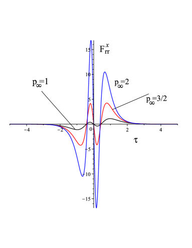
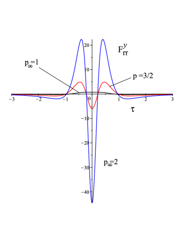
Figure 1: The $x$ and $y$ components of the radiation-reaction force acting on particle 1 (rescaled by $G^{2}m_{1}^{2}m_{2}$, and for $b_{0}=1$), in its incoming rest-frame, plotted as functions of $\tau\equiv\tau_{1}$ for different values of $p_{\infty}$=[1 (black online), 3/2 (red online), 2 (blue online]. ${\mathcal{F}}_{1\,\rm rr}^{x}$ is $\tau$-odd whereas ${\mathcal{F}}_{1\,\rm rr}^{y}$ is $\tau$-even. The asymptotic behaviors of the $x$ and $y$ components of the radiation-reaction forces are ${\mathcal{F}}_{1\,\rm rr}^{x}\sim\frac{\tau}{\tau^{5}}$ and ${\mathcal{F}}_{1\,\rm rr}^{y}\sim\frac{1}{|\tau|^{3}}$.

The midpoint (at $\tau_{1}=0$) values of the force components are

$${\mathcal{F}}_{1\,\rm rr}^{x}(0) = 0\,,$$

$${\mathcal{F}}_{1\,\rm rr}^{y}(0) = \frac{G^{2}m_{1}^{2}m_{2}}{b_{0}^{3}}\left[\frac{(p_{\infty}^{2}+1)(2p_{\infty}^{2}-1)^{2}}{p_{\infty}^{2}}{\mathcal{A}}(p_{\infty})\right.$$ (60)

$$- 2p_{\infty}(2p_{\infty}^{2}-1)\sqrt{p_{\infty}^{2}+1}\ln(p_{\infty}^{2}+1)$$

$$- \left.\frac{12p_{\infty}^{10}-21p_{\infty}^{6}-8p_{\infty}^{4}-2p_{\infty}^{2}+3}{3p_{\infty}(p_{\infty}^{2}+1)^{5/2}}\right]\,.$$

In the limit $\tau_{1}\to\pm\infty$ we find that ${\mathcal{F}}_{1\,\rm rr}^{x}$ vanishes as $\tau_{1}/|\tau_{1}|^{5}$ while ${\mathcal{F}}_{1\,\rm rr}^{y}$ vanishes as $1/|\tau_{1}|^{3}$ with coefficients depending on $p_{\infty}$, namely

$${\mathcal{F}}_{1\,\rm rr}^{x}(\tau_{1}\to\pm\infty) \approx -\frac{G^{2}m_{1}^{2}m_{2}b_{0}\tau_{1}}{|\tau_{1}|^{5}p_{\infty}^{3}}\left[12(2p_{\infty}^{2}+1){\mathcal{A}}(p_{\infty})\right.$$

$$\left.+\frac{(4p_{\infty}^{2}+3)(2p_{\infty}^{2}-1)(p_{\infty}^{2}+1)}{p_{\infty}^{2}}\right]$$

$${\mathcal{F}}_{1\,\rm rr}^{y}(\tau_{1}\to\pm\infty) \approx \frac{2G^{2}m_{1}^{2}m_{2}(2p_{\infty}^{2}-1)\sqrt{1+p_{\infty}^{2}}}{p_{\infty}^{2}|\tau_{1}|^{3}}\times$$ (61)

$$\left[4{\mathcal{A}}(p_{\infty})+\frac{(5p_{\infty}^{2}-3)}{3p_{\infty}^{2}}\right]\,.$$

As shown in Fig. 1 the proper time evolution of the force components is rather complex, and involves (at least) two different time scales which behave differently in the $\gamma\to\infty$ limit. More precisely, while $D^{2}(\tau)=b_{0}^{2}+p_{\infty}^{2}\tau^{2}$ involves the time scale $\tau_{p}=\frac{b_{0}}{p_{\infty}}$, the factor ${\mathcal{D}}^{2}(\tau)/\gamma^{2}=b_{0}^{2}+v^{2}\tau^{2}$, where $v$ was defined in Eq. (V.1), involves the time scale $\tau_{v}=\frac{b_{0}}{v}$. In the low-velocity limit $p_{\infty}\to 0$ the two time scales coincide and measure the usual characteristic Newtonian encounter time. In the high-energy limit $p_{\infty}\to\infty$ we have $\tau_{p}\ll\tau_{v}$, due to relativistic blue-shift effects in retarded interactions. In both limits we can write the two components of the force in terms of the rescaled time variable

$$\hat{\tau}=\frac{\tau}{\tau_{p}}\,.$$ (62)

In the low-velocity limit ($p_{\infty}\to 0$, $v\to 0$) we have

$$\frac{{\mathcal{F}}_{1\,\rm rr}^{x}}{G^{2}m_{1}^{2}m_{2}} = \frac{12}{5}p_{\infty}^{3}\frac{\hat{\tau}}{(1+\hat{\tau}^{2})^{5/2}}\,,$$

$$\frac{{\mathcal{F}}_{1\,\rm rr}^{y}}{G^{2}m_{1}^{2}m_{2}} = \frac{4}{5}p_{\infty}^{3}\frac{2\hat{\tau}^{2}-1}{(1+\hat{\tau}^{2})^{5/2}}\,,$$ (63)

while, in the high-energy limit ($p_{\infty}\to+\infty$, $v\to 1$), we have

$$\frac{{\mathcal{F}}_{1\,\rm rr}^{x}}{G^{2}m_{1}^{2}m_{2}} = -12p_{\infty}^{3}\ln(p_{\infty})\frac{\hat{\tau}}{(1+\hat{\tau}^{2})^{5/2}}\,,$$

$$\frac{{\mathcal{F}}_{1\,\rm rr}^{y}}{G^{2}m_{1}^{2}m_{2}} = 4p_{\infty}^{4}\ln(p_{\infty})\frac{2\hat{\tau}^{2}-1}{(1+\hat{\tau}^{2})^{5/2}}\,.$$ (64)

Note that, apart from different prefactors (including varying signs), each component involves the same function of $\hat{\tau}$ in both limits.

V.2 Moments of the $O(G^{2})$ radiation-reaction force

The integrated value of the force vanishes,

$$\int d\tau_{1}{\mathcal{F}}^{\mu}_{1\rm rr}(\tau_{1})=0\,,$$ (65)

as expected from the conservation of total linear momentum up to the $G^{3}$ level. See also further discussion below.

Let us consider the integrated moments of the radiation-reaction force, i.e., the integrals

$$I_{a}^{(n)\alpha}\equiv\int_{-\infty}^{\infty}d\tau\,\tau^{n}\,{\mathcal{F}}_{a\rm rr}^{\alpha}(\tau)\,.$$ (66)

For $n=0$ we have $I_{1}^{(0)\alpha}=0+O(G^{3})$, in view of Eq. (65). As we shall see below of particular importance is the first moment $n=1$ which is found to be

$$I_{1}^{(1)t} = 0\,,$$

$$I_{1}^{(1)x} = \frac{G^{2}m_{1}^{2}m_{2}}{b_{0}}\,c_{I}(v)\,{\mathcal{I}}(v)\,,$$

$$I_{1}^{(1)y} = 0\,.$$ (67)

Here, we defined (remembering the definition of $v$, Eq. (V.1)),

$$c_{I}(v)\equiv\frac{1+v^{2}}{v\sqrt{1-v^{2}}}=\frac{2\gamma^{2}-1}{\sqrt{\gamma^{2}-1}}\,,$$ (68)

and, consistently with Eqs. (4.7) and (4.8) of Ref. Damour:2020tta ,

$${\mathcal{I}}(v) \equiv -\frac{16}{3}+\frac{2}{v^{2}}+\frac{2(3v^{2}-1)}{v^{3}}{\mathcal{A}}(v)\,,$$

$${\mathcal{A}}(v) \equiv {\rm arctanh}v=\frac{1}{2}\ln\frac{1+v}{1-v}$$ (69)

$$= 2{\rm arcsinh}\left(\sqrt{\frac{\gamma-1}{2}}\right)\,.$$

Note that ${\mathcal{A}}(v)$ is numerically equal to the ${\mathcal{A}}(p_{\infty})$ defined in Eq. (56) above.

In terms of $p_{\infty}$ our results read

$$I_{1}^{(1)x} = \frac{2G^{2}m_{1}^{2}m_{2}(2p_{\infty}^{2}+1)}{bp_{\infty}^{3}}\left[\frac{(2p_{\infty}^{2}-1)\sqrt{1+p_{\infty}^{2}}}{p_{\infty}}\times\right.$$ (70)

$$\left.\times{\mathcal{A}}(p_{\infty})-\frac{5p_{\infty}^{2}-3}{3}\right]\,.$$

Recalling that $e_{x}^{\mu}=\hat{b}_{12}^{\mu}$ we can rewrite the above relation in a covariant form

$$I_{1}^{(1)\mu}=\frac{G^{2}m_{1}^{2}m_{2}}{b_{12}^{2}}b_{12}^{\mu}c_{I}(v)\,{\mathcal{I}}(v)\,.$$ (71)

V.3 Schott term in the radiation-reaction force

We have seen above that ${\mathcal{F}}^{\mu}_{1\rm rr}(\tau_{1})$ starts at $O(G^{2})$ but that

$$\int d\tau_{1}{\mathcal{F}}^{\mu}_{1\rm rr}(\tau_{1})=O(G^{3})\,.$$ (72)

This situation is similar to the well-known structure of the Abraham-Lorentz-Dirac radiation reaction force for a test-charge particle in an external field, namely (with $\cdot\equiv\frac{d}{d\tau}$)

$$m_{1}\frac{du^{\mu}}{d\tau}=\frac{2}{3}e_{1}^{2}(\ddot{u}^{\mu}-\dot{u}^{2}u^{\mu})+F^{\mu}_{\rm ext}\equiv{\mathcal{F}}^{\mu}_{\rm rr}+F^{\mu}_{\rm ext}\,.$$ (73)

Only the second term, $-\frac{2}{3}e_{1}^{2}\dot{u}^{2}u^{\mu}$, in ${\mathcal{F}}^{\mu}_{\rm rr}$ is linked to the emission of radiation. Indeed,

$$P^{\mu}_{\rm rad}(\tau)=+\frac{2}{3}e_{1}^{2}\int_{-\infty}^{\tau}d\tau\dot{u}^{2}u^{\mu}\,,$$ (74)

or

$$\frac{dP^{\mu}_{\rm rad}}{d\tau}=+\frac{2}{3}e_{1}^{2}\dot{u}^{2}u^{\mu}\,.$$ (75)

The first term $\frac{2}{3}e_{1}^{2}\ddot{u}^{\mu}$ in ${\mathcal{F}}^{\mu}_{\rm rr}$ is a total time derivative. It was interpreted by Schott Schott_book as part of the interaction energy between the charge and the field. Defining

$$P^{\mu}_{\rm kin}=m_{1}u^{\mu}\,,$$ (76)

and

$$P^{\mu}_{\rm Schott}=-\frac{2}{3}e_{1}^{2}\dot{u}^{\mu}$$ (77)

Eq. (73) reads

$$\frac{dP^{\mu}_{\rm tot}}{d\tau}=F^{\mu}_{\rm ext}\,,$$ (78)

where

$$P^{\mu}_{\rm tot}=P^{\mu}_{\rm kin}+P^{\mu}_{\rm Schott}+P^{\mu}_{\rm rad}\,.$$ (79)

Eqs. (78) and (79) exhibit the role of the Schott momentum as a necessary additional contribution in the energy-momentum balance between external force, particle and radiation. If the external force is due to the electromagnetic interaction between the test charge $e_{1}$ and another (heavy) charge $e_{2}$ (with $e_{2}\sim e_{1}$), the Schott momentum and the radiated momentum scale differently with the coupling constant $\alpha\equiv e_{1}e_{2}\sim e_{1}^{2}$. While $P^{\mu}_{\rm rad}=O(\alpha^{3})$, the Schott momentum scales with a lower power of $\alpha$: $P^{\mu}_{\rm Schott}=O(\alpha^{2})$. Correspondingly, in the radiation-reaction force, the Schott term is $O(\alpha^{2})$, while the “proper” radiation-reaction term, $-\frac{2}{3}e_{1}^{2}\dot{u}^{2}u^{\mu}$, is proportional to $\alpha^{3}$.

The latter situation is analogous to the structure of the radiation-reaction force in gravity, with the analogy $\alpha\leftrightarrow G$. The $O(G^{2})$ radiation-reaction force discussed in the present paper is analogous to the Schott force $\frac{2}{3}e_{1}^{2}\ddot{u}$. It would be natural to decompose the gravitational radiation-reaction force as

$${\mathcal{F}}^{\mu}_{\rm rr}=-\frac{dP^{\mu}_{\rm Schott}}{d\tau}+{\mathcal{F}}^{\mu}_{\rm rr\,proper}\,,$$ (80)

with $P^{\mu}_{\rm Schott}=O(G^{2})$ and ${\mathcal{F}}^{\mu}_{\rm rr\,proper}=O(G^{3})$. In this relation only be ${\mathcal{F}}^{\mu}_{\rm rr\,proper}$ would be responsible for the radiative loss of linear momentum of each particle. Our present treatment is limited to $O(G^{2})$ accuracy, and therefore only gives access to $P^{\mu}_{\rm Schott}$ to this order. Integrating

$${\mathcal{F}}^{\mu}_{1\,\rm rr}(\tau_{1})=-\frac{d}{d\tau_{1}}P^{\mu}_{1\,\rm Schott}+O(G^{3})\,,$$ (81)

we find that the two components of $P^{\mu}_{1\,\rm Schott}(\tau_{1})$,

$$P^{\mu}_{1\,\rm Schott}(\tau_{1})=P^{x}_{1\,\rm Schott}(\tau_{1})e_{x}^{\mu}+P^{y}_{1\,\rm Schott}(\tau_{1})e_{y}^{\mu}\,,$$ (82)

are given, at order $G^{2}$, by the following expressions

$$\frac{P_{1\,\rm Schott}^{x\,G^{2}}}{G^{2}m_{1}^{2}m_{2}} = -2\frac{b_{0}}{D^{3}}(1+2p_{\infty}^{2})\ln\left(\frac{{\mathcal{D}}^{2}}{D^{2}}\right)-\frac{3}{4b_{0}^{2}p_{\infty}}(4+5p_{\infty}^{2}){\rm arctan}\left(\frac{p_{\infty}b_{0}}{D}\right)$$

$$+ \frac{b_{0}(4p_{\infty}^{4}-1)}{p_{\infty}^{3}D^{3}}\left[\sqrt{1+p_{\infty}^{2}}{\rm arcsinh}(p_{\infty})-p_{\infty}\right]$$

$$+ \frac{1}{Db_{0}p_{\infty}}\left[2(1+6p_{\infty}^{2}+4p_{\infty}^{4})-\frac{1}{4}(28+84p_{\infty}^{2}+47p_{\infty}^{4})\frac{D^{2}}{{\mathcal{D}}^{2}}\right.$$

$$+ \left.\frac{1}{6}(74+136p_{\infty}^{2}+65p_{\infty}^{4})\frac{D^{4}}{{\mathcal{D}}^{4}}-\frac{2}{3}(1+p_{\infty}^{2})(17+11p_{\infty}^{2})\frac{D^{6}}{{\mathcal{D}}^{6}}+4(1+p_{\infty}^{2})^{2}\frac{D^{8}}{{\mathcal{D}}^{8}}\right]\,,$$

$$\frac{P_{1\,\rm Schott}^{y\,G^{2}}}{G^{2}m_{1}^{2}m_{2}\tau} = \frac{2p_{\infty}(2p_{\infty}^{2}-1)\sqrt{1+p_{\infty}^{2}}}{D^{3}}\ln\left(\frac{{\mathcal{D}}^{2}}{D^{2}}\right)+\frac{\sqrt{1+p_{\infty}^{2}}(2p_{\infty}^{2}-1)^{2}}{p_{\infty}^{2}D^{3}}[-\sqrt{1+p_{\infty}^{2}}{\rm arcsinh}(p_{\infty})+p_{\infty}]$$

$$+ \frac{\sqrt{1+p_{\infty}^{2}}}{D^{3}}\left[-2p_{\infty}(4p_{\infty}^{2}-1)\frac{D^{2}}{{\mathcal{D}}^{2}}+p_{\infty}(6p_{\infty}^{2}-5)\frac{D^{4}}{{\mathcal{D}}^{4}}+\frac{2}{3}p_{\infty}(11+8p_{\infty}^{2})\frac{D^{6}}{{\mathcal{D}}^{6}}-4p_{\infty}(1+p_{\infty}^{2})\frac{D^{8}}{{\mathcal{D}}^{8}}\right]\,.$$

Remembering the definitions of $D(\tau_{1})$ (see the first of Eqs. (V.1)) and ${\mathcal{D}}(\tau_{1})$ (see the second of Eqs. (V.1)), one sees that $P_{\rm Schott}^{x\,G^{2}}$ is an even function of $\tau$ while $P_{\rm Schott}^{y\,G^{2}}$ is an odd function of $\tau$. In addition, when $\tau\to\pm\infty$, both components of $P_{1\,\rm Schott}^{y\,G^{2}}$ tend to zero. More precisely:

$$P_{1\,\rm Schott}^{x\,G^{2}}\sim\frac{1}{|\tau|^{3}}\,,\qquad P_{1\,\rm Schott}^{y\,G^{2}}\sim\frac{\tau}{|\tau|^{3}}\,.$$ (84)

In the following we will study the role of the radiation-reaction force ${\mathcal{F}}_{1\,\rm rr}^{\mu}$ on the conservation (respectively, dissipation) of the linear momentum (respectively, angular momentum) of the system.

VI Evolution of Noetherian quantities at $O(G^{2})$

As discussed in Section IV the time-symmetric dynamics of two masses admits conserved Noetherian quantities associated with the Poincaré symmetry of its Fokker action. As explicitly shown, at the 1PM level, in Eqs. (IV) the Noetherian conserved quantities $P_{\rm sys}^{\mu}$ and $J_{\rm sys}^{\mu\nu}$ are the sum of kinematical quantities and interaction contributions. The existence of these conserved quantities for the time-symmetric dynamics, and the decomposition of the retarded force given in Eq. (48), show that when considering the retarded dynamics the non-conservation of $P_{\rm sys}^{\mu}$ and $J_{\rm sys}^{\mu\nu}$ will only come from the additional term ${\mathcal{F}}_{a\,\rm rr}^{\mu}$ in the equations of motion. A way to make this explicit would be (following Lagrange’s method of variation of constants) to express $P_{\rm sys}^{\mu}$ and $J_{\rm sys}^{\mu\nu}$ as functions of four quantities $z_{1}^{\mu}$, $u_{1}^{\mu}$, $z_{2}^{\mu}$ and $u_{2}^{\mu}$, which can serve as “initial” conditions determining a solution of the time-symmetric equations of motion. Then, starting from the functions $P_{\rm sys}^{\mu}(z_{1},u_{1},z_{2},u_{2})$ and $J_{\rm sys}^{\mu\nu}(z_{1},u_{1},z_{2},u_{2})$ we get evolution equations for these quantities under the retarded dynamics of the form

$$dP_{\mu}^{\rm sys} = \sum_{a}\frac{\partial P_{\mu}^{\rm sys}}{\partial u_{a}^{\lambda}}\frac{{\mathcal{F}}^{\lambda}_{a\,\rm rr}(\tau_{a})}{m_{a}}\frac{d\tau_{a}}{d\sigma}d\sigma\,,$$

$$dJ_{\mu\nu}^{\rm sys} = \sum_{a}\frac{\partial J_{\mu\nu}^{\rm sys}}{\partial u_{a}^{\lambda}}\frac{{\mathcal{F}}^{\lambda}_{a\,\rm rr}(\tau_{a})}{m_{a}}\frac{d\tau_{a}}{d\sigma}d\sigma\,.$$ (85)

Here, $\sigma$ parametrizes a way to correlate the common sliding of the data $z_{a},u_{a}$ along the two world lines. For instance, one could use (as is done when dealing with the PN-expanded dynamics) a coordinate time $t$ is some Lorentz frame.

When working in a PM-expanded way, the facts that the Noetherian quantities differ from kinematical quantities by $O(G)$ interaction contributions and that the radiation-reaction force starts at order $O(G^{2})$ allows us to write the following $G^{2}$-accurate evolution equations

$$dP_{\mu}^{\rm sys} = \sum_{a}\frac{\partial P_{\mu}^{\rm kin}}{\partial u_{a}^{\lambda}}\frac{{\mathcal{F}}^{\lambda}_{a\,\rm rr}(\tau_{a})}{m_{a}}\frac{d\tau_{a}}{d\sigma}d\sigma+O(G^{3})\,,$$

$$dJ_{\mu\nu}^{\rm sys} = \sum_{a}\frac{\partial J_{\mu\nu}^{\rm kin}}{\partial u_{a}^{\lambda}}\frac{{\mathcal{F}}^{\lambda}_{a\,\rm rr}(\tau_{a})}{m_{a}}\frac{d\tau_{a}}{d\sigma}d\sigma+O(G^{3})\,,$$ (86)

i.e., explicitly

$$dP^{\mu}_{\rm sys} = \sum_{a}{\mathcal{F}}^{\mu}_{a\,\rm rr}(\tau_{a})\frac{d\tau_{a}}{d\sigma}d\sigma+O(G^{3})\,,$$

$$dJ^{\mu\nu}_{\rm sys} = \sum_{a}(z_{a}^{\mu}{\mathcal{F}}^{\nu}_{a\,\rm rr}(\tau_{a})-z_{a}^{\nu}{\mathcal{F}}^{\mu}_{a\,\rm rr}(\tau_{a}))\frac{d\tau_{a}}{d\sigma}d\sigma$$ (87)

$$+ O(G^{3})\,.$$

VI.1 Linear momentum

In Appendix C we evaluate at 1PM accuracy the interaction contribution to the total linear momentum of a binary system. Our computation explicitly shows that the interaction contribution to $P_{\mu}^{\rm sys}$ vanishes both in the asymptotic incoming and outgoing states. In addition, it also gives an explicit check of the conservation of $P_{\mu}^{\rm sys}$ under the 1PM dynamics (which is time-symmetric by itself at this order, as discussed above).

When working at the 2PM accuracy with the retarded dynamics, the first equation in Eqs. (VI) says that the total change during scattering of the Noetherian conserved momentum of the system is given by

$$[P_{\rm sys}^{\mu}]_{-\infty}^{+\infty}=\sum_{a}\int d\tau_{a}{\mathcal{F}}^{\mu}_{a\,\rm rr}(\tau_{a})+O(G^{3})\,,$$ (88)

where we adopted the notation $[Q]_{-\infty}^{+\infty}\equiv Q(+\infty)--Q(-\infty)$.

Using Eq. (72) this yields

$$[P^{\rm sys}]_{-\infty}^{+\infty}=O(G^{3})\,.$$ (89)

In addition, using the fact that the interaction contribution to $P^{\rm sys}$ vanishes in the asymptotic states, Eq. (89), we get

$$[m_{1}u_{1}+m_{2}u_{2}]_{-\infty}^{+\infty}=O(G^{3})\,.$$ (90)

VI.2 Angular momentum

In Appendix D we evaluate at 1PM accuracy the interaction contribution to the total angular momentum of a system to explicitly check its conservation under the 1PM dynamics (which is time-symmetric by itself at this order, as discussed above). Contrary to the case of the linear momentum, the interaction contribution to the angular momentum does not vanish in the asymptotic limits $t\to\pm\infty$. However, it exactly compensates opposite contributions (linked to the asymptotic logarithmic behaviors of the world lines) present in the kinematical part of the angular momentum.

The non-conserved, and asymptotically non-vanishing, contributions to $J_{\mu\nu}^{\rm kin}$ were called “scoot terms” in Refs. Gralla:2021eoi ; Gralla:2021qaf . The scoot contributions to $J_{\mu\nu}^{\rm kin}$ are not Lorentz-invariant (see Eqs. (150), (151) and (152) in Appendix D). Our computations in Appendix D explicitly show that these non Lorentz-invariant and non-conserved scoot kinematical contributions cancel against corresponding (Fokker) interaction contributions to the total angular momentum.

The final (manifestly Poincaré-invariant, and conserved) result for $J_{\mu\nu}^{\rm sys}(\tau_{1},\tau_{2})=J_{\mu\nu}^{\rm kin}(\tau_{1},\tau_{2})+J_{\mu\nu}^{\rm int}(\tau_{1},\tau_{2})$ is

$$J_{\mu\nu}^{\rm sys}(\tau_{1},\tau_{2}) = \left((z_{1}(0)+\delta^{G}z_{1})\wedge p_{1}^{-}\right)_{\mu\nu}$$ (91)

$$+ \left((z_{2}(0)+\delta^{G}z_{2})\wedge p_{2}^{-}\right)_{\mu\nu}$$

$$+ O(G^{2})\,,$$

where

$$\delta^{G}z_{1}^{\mu} = +Gm_{2}\frac{2\gamma^{2}-1}{(\gamma^{2}-1)}\hat{b}_{12}^{\mu}\,,$$

$$\delta^{G}z_{2}^{\mu} = -Gm_{1}\frac{2\gamma^{2}-1}{(\gamma^{2}-1)}\hat{b}_{12}^{\mu}\,.$$ (92)

In other words, defining $b^{\mu}_{a\,\rm in}\equiv z_{a}^{\mu}(0)+\delta^{G}z_{a}^{\mu}$, we can write $J_{\mu\nu}^{\rm sys}(\tau_{1},\tau_{2})$ as

$$J_{\mu\nu}^{\rm sys}(\tau_{1},\tau_{2}) = (b_{1\,\rm in}\wedge p_{1}^{-})_{\mu\nu}$$ (93)

$$+ (b_{2\,\rm in}\wedge p_{2}^{-})_{\mu\nu}$$

$$+ O(G^{2})\,,$$

The modulus of the difference $b^{\mu}_{1\,\rm in}-b^{\mu}_{2\,\rm in}$ is equal to the incoming impact parameter $b_{\rm in}$ defined in Eq. (14).

When working at the 2PM accuracy with the retarded dynamics, the second equation in Eqs. (VI) says that the total change during scattering of the Noetherian conserved angular momentum of the system is given by

$$[J_{\rm sys}^{\mu\nu}]_{-\infty}^{+\infty}=\sum_{a}\int d\tau_{a}(z_{a}(\tau_{a})\wedge{\mathcal{F}}_{a\,\rm rr}(\tau_{a}))^{\mu\nu}+O(G^{3})\,.$$ (94)

At order $G^{2}$ it is enough to insert the straight line approximation for $z_{a}^{\mu}(\tau_{a})$ in Eq. (94),

$$[J_{\rm sys}^{\mu\nu}]_{-\infty}^{+\infty}=\sum_{a}\int d\tau_{a}[(z_{a}(0)+\bar{u}_{a}\tau_{a})\wedge{\mathcal{F}}_{a\,\rm rr}(\tau_{a})]^{\mu\nu}+O(G^{3})\,.$$ (95)

The contribution proportional to $z_{a}(0)$ vanishes because of Eq. (65). By contrast, the contribution proportional to $\bar{u}_{a}\tau_{a}$ yields a term proportional to the first moment of the radiation-reaction force:

$$I_{a}^{(1)\mu}=\int d\tau_{a}\tau_{a}{\mathcal{F}}_{a\,\rm rr}^{\mu}(\tau_{a})\,,$$ (96)

leading to

$$[J_{\rm sys}^{\mu\nu}]_{-\infty}^{+\infty}=\sum_{a}[\bar{u}_{a}\wedge I_{a}^{(1)}]^{\mu\nu}+O(G^{3})\,.$$ (97)

We have evaluated the moment $I_{a}^{(1)\mu}$ in Eq. (66) above. This yields the central result of the present paper :

$$[J_{\rm sys}^{\mu\nu}]_{-\infty}^{+\infty}=\Delta J_{1}^{\mu\nu}+\Delta J_{2}^{\mu\nu}+O(G^{3})\,,$$ (98)

where

$$\Delta J_{1}^{\mu\nu} = \bar{u}_{1}^{\mu}\wedge\int d\tau_{1}\tau_{1}{\mathcal{F}}_{1\,\rm rr}^{\nu}(\tau_{1})$$ (99)

$$= \frac{G^{2}m_{1}m_{2}}{b_{12}^{2}}\,c_{I}(v)\,{\mathcal{I}}(v)\,[p_{1}\wedge b_{12}]^{\mu\nu}\,,$$

and

$$\Delta J_{2}^{\mu\nu} = \bar{u}_{2}^{\mu}\wedge\int d\tau_{2}\tau_{2}{\mathcal{F}}_{1\,\rm rr}^{\nu}(\tau_{2})$$ (100)

$$= \frac{G^{2}m_{1}m_{2}}{b_{12}^{2}}\,c_{I}(v)\,{\mathcal{I}}(v)\,[p_{2}\wedge b_{21}]^{\mu\nu}\,,$$

leading to

$$[J_{\rm sys}^{\mu\nu}]_{-\infty}^{+\infty}=\frac{G^{2}m_{1}m_{2}}{b_{12}^{2}}\,c_{I}(v)\,{\mathcal{I}}(v)\,[(p_{1}-p_{2})\wedge b_{12}]^{\mu\nu}+O(G^{3})\,.$$ (101)

This total variation in the Noetherian angular momentum of the binary system coincides with the opposite of the $O(G^{2})$ integrated radiative flux of angular momentum computed in Refs. Damour:2020tta ; Manohar:2022dea . It was obtained here by a direct equations-of-motion-based approach (similar to the lowest PN order of Ref. Damour:1981bh ) without ever appealing to a balance with fluxes of angular momentum in the radiation zone. See Concluding Remarks for further discussion.

VI.3 Radiation-reaction-induced shifts in the world lines of the two bodies

In view of the conservative-plus-dissipative decomposition of the equations of motion

$$m_{a}\frac{d^{2}}{d\tau_{a}^{2}}z_{a}^{\mu}(\tau_{a})={\mathcal{F}}_{aR}^{\mu}(\tau_{a})={\mathcal{F}}_{aS}^{\mu}(\tau_{a})+{\mathcal{F}}_{a\,\rm rr}^{\mu}(\tau_{a})\,,$$ (102)

one can, at order $G^{2}$, accordingly decompose the solution world lines for the retarded dynamics in conservative and radiation-reaction parts:

$$z_{a}^{\mu}(\tau_{a})=z_{aS}^{\mu}(\tau_{a})+z_{a\,\rm rr}^{\mu}(\tau_{a})+O(G^{3})\,.$$ (103)

Here, $z_{aS}^{\mu}(\tau_{a})$ is the solution of the conservative dynamics while the radiation-reaction shift $z_{a\,\rm rr}^{\mu}(\tau_{a})$ is the solution of

$$m_{a}\frac{d^{2}}{d\tau_{a}^{2}}z_{a\,\rm rr}^{\mu}(\tau_{1})={\mathcal{F}}_{a\,\rm rr}^{\mu}(\tau_{1})\,.$$ (104)

Here and below we suppress the $O(G^{3})$ error terms. Taking into account Eq. (81) we can integrate Eq. (104) once obtaining

$$m_{a}\frac{d}{d\tau_{a}}z_{a\,\rm rr}^{\mu}(\tau_{a})=-P_{a\,\rm Schott}^{\mu}(\tau_{a})\,,$$ (105)

where we imposed the boundary condition that $\frac{dz_{a\,\rm rr}^{\mu}(\tau_{a})}{d\tau_{a}}$ vanishes in the incoming state. As we have shown above that $P_{a\,\rm Schott}^{\mu}(\tau_{a})$ vanishes in both asymptotic limits, $\tau_{a}\to\pm\infty$, we see that $\frac{dz_{a\,\rm rr}(\tau_{a})}{d\tau_{a}}^{\mu}$ vanishes also in the outgoing state.

Integrating now Eq. (105) we find that the radiation-reaction-induced shift of each world line is equal to

$$z_{a\,\rm rr}^{\mu}(\tau_{a})=-\frac{1}{m_{a}}\int_{-\infty}^{\tau_{a}}d\bar{\tau}_{a}P_{a\,\rm Schott}^{\mu}(\bar{\tau}_{a})\,,$$ (106)

where we imposed the condition that $z_{a\,\rm rr}^{\mu}(\tau_{a})$ vanishes in the incoming state.

Taking the limit $\tau_{a}\to+\infty$ and using Eqs. (V.2) we find that the radiation-reaction shifts in the outgoing world lines are given by

$$[z_{1\,\rm rr}^{\mu}]^{+\infty} = -\alpha\,\hat{b}_{12}^{\mu}\,,$$

$${}[z_{2\,\rm rr}^{\mu}]^{+\infty} = -\alpha\,\hat{b}_{21}^{\mu}=+\alpha\,\hat{b}_{12}^{\mu}\,,$$ (107)

where

$$\alpha\equiv\frac{G^{2}m_{1}m_{2}}{b_{12}}c_{I}(v)\,{\mathcal{I}}(v)\,.$$ (108)

Note that $\alpha$ is positive so that each world line is shifted towards the other world line.

These shifts can be interpreted in terms of an outgoing impact parameter $b^{\rm out}$ that differs (because of radiation-reaction effects) from the incoming one $b^{\rm in}$ (such that $J_{\rm c.m.}^{\rm in}=b^{\rm in}P_{\rm c.m.}^{\rm in}$, see Eq.(13)), by

$$b^{\rm out}=b^{\rm in}-2\alpha\,.$$ (109)

Such a shift implies a c.m. angular momentum decrease

$$J_{\rm c.m.}^{\rm out}=J_{\rm c.m.}^{\rm in}-2\alpha(v)P_{\rm c.m.}\,,$$ (110)

which agrees with the result of Ref. Damour:2020tta , and is easily seen to be compatible with the Poincaré-covariant result, Eq. (101). We leave to future investigations a discussion of the relation of the individual radiation-reaction worldline shifts, Eqs. (VI.3), to the recent corresponding results of Ref. DiVecchia:2022piu .

VII Concluding remarks

We computed the effect of radiation-reaction at the second post-Minkowskian order $O(G^{2})$. The radiation-reaction force was defined by comparing the 2PM-accurate retarded dynamics, Eqs. (1) and (18), to its time-symmetric counterparts, Eqs. (32) and (33). This led to the definition (49) of the radiation-reaction force ${\mathcal{F}}_{a\,\rm rr}^{\mu}(\tau_{a})$. The explicit value of ${\mathcal{F}}_{1\,\rm rr}^{\mu}(\tau_{1})$ is given in subsection V.1.

Capitalizing on the existence of Noetherian conserved quantities, under the Fokker-Wheeler-Feynman-type time-symmetric dynamics for the binary system, $P_{\rm sys}^{\mu}(z_{1},u_{1},z_{2},u_{2})$ and $J_{\rm sys}^{\mu\nu}(z_{1},u_{1},z_{2},u_{2})$, we used the method of variation of constants to compute the evolution of $P_{\rm sys}^{\mu}(z_{1},u_{1},z_{2},u_{2})$ and $J_{\rm sys}^{\mu\nu}(z_{1},u_{1},z_{2},u_{2})$ under the retarded dynamics, see Eqs. (VI) and (VI).

Consistently with current knowledge we found that the total linear momentum of the system is conserved at the 2PM order. By contrast, we found that the total variation of the angular momentum of the system under the retarded dynamics was given by Eq. (101), namely

$$J_{\rm sys,out}^{\mu\nu}-J_{\rm sys,in}^{\mu\nu} = \frac{G^{2}m_{1}m_{2}}{b_{12}^{2}}\,c_{I}(v){\mathcal{I}}(v)[(p_{1}-p_{2})\wedge b_{12}]^{\mu\nu}$$ (111)

$$+ O(G^{3})\,,$$

where $c_{I}(v)$ and ${\mathcal{I}}(v)$ are respectively defined in Eqs. (68) and (V.2).

The crucial point in our derivation of the result (111) is that it was obtained here directly from the (near-zone, retarded) mechanical equations of motion of the two world lines, without ever evaluating fluxes of angular momentum in the radiation zone. This allows us to by-pass the subtleties linked to the definition of angular momentum at future null infinity with its attendant Bondi-Metzner-Sachs-related super-translation ambiguities Veneziano:2022zwh ; Porrati2022 .

Our derivation is a generalization to all powers of $v/c$ of the lowest order result of Ref. Damour:1981bh which was also directly based on the $G^{2}$-accurate retarded equations of motion of the binary system.

We expect that our direct equations-of-motion-based approach can be extended to the $G^{3}$ level, where the Fokker action should be well defined. By contrast, several arguments (presence of tails Bini:2021gat ; Dlapa:2022lmu ; Bini:2022enm , effects proportional the square of ${\mathcal{F}}_{a\,\rm rr}^{\mu}$) suggest that the $G^{4}$ level will introduce new subtleties.

Appendix A Definition of retarded/advanced quantities

Advanced and retarded definitions can be treated together with an indicator $\epsilon$, where $\epsilon=1$ in the retarded case and $\epsilon=-1$ in the advanced one. Using the notation of Ref. Bel:1981be , which deals both with a generic field point $x$ and several world line points ($z_{1}$, $\hat{z}_{2\epsilon}$, etc.), we have 

$$w_{\epsilon} = u_{1}\cdot u_{2\epsilon}\,,\qquad\qquad\qquad\omega_{\epsilon}=u_{1}\cdot\hat{u}_{2\epsilon}$$

$$r_{\epsilon} = -\epsilon u_{1}\cdot(x-z_{1})\,,\qquad\,\,\,\,\rho_{\epsilon}=-\epsilon(z_{1}-\hat{z}_{1\epsilon})\cdot\hat{u}_{2\epsilon}$$

$$n_{\epsilon} = \frac{1}{r_{\epsilon}}P(u_{1})(x-z_{1})\,,\qquad\nu_{\epsilon}=\frac{1}{\rho_{\epsilon}}P(\hat{u}_{2\epsilon})(z_{1}-\hat{z}_{2\epsilon})\,,$$

to which one has to add

$$A_{\epsilon}^{\alpha} = \frac{1}{\rho_{\epsilon}}[P(u_{1})(z_{1}-\hat{z}_{2\epsilon})]^{\alpha}\,,\qquad A_{\epsilon}\equiv|A_{\epsilon}^{\alpha}|\,,$$

$$v_{\epsilon}^{\alpha} = (P(u_{1})u_{2\epsilon})^{\alpha}\,.$$ (113)

Here, $P(u)^{\alpha}{}_{\beta}=\delta^{\alpha}_{\beta}+u^{\alpha}u_{\beta}$ is the projector orthogonal to the unit timelike vector $u$, $u\cdot u=-1$. Since $z_{1}^{\alpha}-\hat{z}_{2\epsilon}^{\alpha}$ is a null vector

$$z^{\alpha}-\hat{z}_{2\epsilon}^{\alpha}=(P(u_{1})(z_{1}-\hat{z}_{2\epsilon}))^{\alpha}+u_{1}^{\alpha}\,[u_{1}\cdot(z_{1}-\hat{z}_{2\epsilon})]\,,$$ (114)

with

$$|(P(u_{1})(z_{1}-\hat{z}_{2\epsilon}))^{\alpha}|=|u_{1}\cdot(z_{1}-\hat{z}_{2\epsilon})|\,,$$ (115)

that is

$$\epsilon\rho_{\epsilon}A_{\epsilon}=u_{1}\cdot(z_{1}-\hat{z}_{2\epsilon})\,,$$ (116)

where one has taken into account that for the retarded point the component of $(z_{1}-\hat{z}_{2\epsilon})$ along $u_{1}$ is positive whereas for the advanced point the latter is negative. Finally, note that the decomposition of the null vector $z_{1}^{\mu}-\hat{z}_{2\epsilon}^{\mu}$ with respect to the $u_{1}^{\mu}$ time axis can be written in the following two ways

$$z_{1}^{\mu}-\hat{z}_{2\epsilon}^{\mu} = \rho_{\epsilon}(A^{\mu}_{\epsilon}+\epsilon u_{1}^{\mu}A_{\epsilon})\,,$$ (117)

$$= \rho_{\epsilon}A_{\epsilon}(N_{\epsilon}^{\mu}+\epsilon u_{1}^{\mu})=B_{\epsilon}(N_{\epsilon}^{\mu}+\epsilon u_{1}^{\mu})\,,$$

where we introduced the unit spatial vector

$$N_{\epsilon}^{\mu}\equiv\frac{A_{\epsilon}^{\mu}}{A_{\epsilon}}\,,$$ (118)

and the modulus

$$B_{\epsilon}\equiv\rho_{\epsilon}A_{\epsilon}\,.$$ (119)

Appendix B Notation, definitions and a list of useful relations

Let us consider the definition (II) of $D(\tau)$ and $S(\tau)$. A number of useful relations can be found, e.g. $S(\tau)S(-\tau)=1$, as well as

$$I_{n}=\int_{-\infty}^{\infty}\frac{d\tau}{D^{n}(\tau)}=\frac{b_{0}^{1-n}}{\sqrt{\gamma^{2}-1}}\frac{\Gamma(\frac{n-1}{2})}{\Gamma(\frac{n}{2})}\,.$$ (120)

Of special interest are then the values of the functions $D(\tau^{\prime}_{\epsilon}(\tau))$ and $S(\tau^{\prime}_{\epsilon}(\tau))$ where

$$\tau^{\prime}_{\epsilon}(\tau)=\gamma\tau-\epsilon D(\tau)\,.$$ (121)

We find

$$D(\tau^{\prime}_{\epsilon}(\tau)) = \gamma D(\tau)-\epsilon(\gamma^{2}-1)\tau=A_{\epsilon}\rho_{\epsilon}=B_{\epsilon}$$

$$S(\tau^{\prime}_{\epsilon}(\tau)) = \frac{\sqrt{\gamma^{2}-1}}{b_{0}}[\gamma\tau-\epsilon D(\tau)]+\frac{A_{\epsilon}\rho_{\epsilon}}{b_{0}}\,,$$ (122)

where all quantities in these expressions ($\tau^{\prime}_{\epsilon}$, $A_{\epsilon}$, $\rho_{\epsilon}$, etc.) are meant to be the corresponding zeroth-PM-order values. Similarly, the following (less evident) relations hold

$$S(\gamma\tau+D(\tau))S(\gamma\tau-D(\tau)) = S(\tau)^{2}\,,$$

$$D(\gamma\tau+D(\tau))D(\gamma\tau-D(\tau)) = \gamma^{2}D^{2}(\tau/\gamma)\,,$$

$$D(\gamma\tau+D(\tau))+D(\gamma\tau-D(\tau)) = 2\gamma D(\tau)\,,$$

$$D(\gamma\tau+D(\tau))-D(\gamma\tau-D(\tau)) = 2\tau(\gamma^{2}-1)\,,$$ (123)

also implying

$$D(\gamma\tau+D(\tau)) = \gamma D(\tau)+\tau(\gamma^{2}-1)\,,$$

$$D(\gamma\tau-D(\tau)) = \gamma D(\tau)-\tau(\gamma^{2}-1)\,,$$ (124)

and

$$(\gamma\tau+D(\tau))D(\gamma\tau-D(\tau))$$

$$+(\gamma\tau-D(\tau))D(\gamma\tau+D(\tau))=2\tau D(\tau)\,.$$ (125)

Appendix C Linear momentum at $O(G)$: computational details

In Eq. (IV) (and related Eqs. (IV) and (IV)) we distinguished a kinematical and an interaction part in the total linear momentum. A direct evaluation at order $O(G)$ of the kinematical part leads to

$$P_{\rm kin}^{\mu}(\tau_{1},\tau_{2})=Ap_{1}^{\mu}+Bp_{2}^{\mu}+Ce_{x}^{\mu}\,,$$ (126)

with

$$A = 1+Gm_{2}\frac{\gamma(2\gamma^{2}-3)}{\gamma^{2}-1}\left(-\frac{\gamma}{D(\tau_{1})}+\frac{1}{D(\tau_{2})}\right)\,,$$

$$B = 1-Gm_{1}\frac{\gamma(2\gamma^{2}-3)}{\gamma^{2}-1}\left(\frac{\gamma}{D(\tau_{2})}-\frac{1}{D(\tau_{1})}\right)\,,$$

$$C = -\frac{Gm_{1}m_{2}}{b_{0}}(2\gamma^{2}-1)\left(\frac{\tau_{1}}{D(\tau_{1})}-\frac{\tau_{2}}{D(\tau_{2})}\right)\,.$$ (127)

The interaction part instead reduces to

$$P_{\rm int}^{\mu}(\tau_{1},\tau_{2}) = Gm_{2}p_{1}^{\mu}\frac{\gamma(2\gamma^{2}-3)}{(\gamma^{2}-1)}\left(\frac{\gamma}{D(\tau_{1})}-\frac{1}{D(\tau_{2})}\right)$$

$$+ Gm_{1}p_{2}^{\mu}\frac{\gamma(2\gamma^{2}-3)}{(\gamma^{2}-1)}\left(\frac{\gamma}{D(\tau_{2})}-\frac{1}{D(\tau_{1})}\right)$$

$$+ 2Gm_{1}m_{2}(2\gamma^{2}-1)(b_{1}^{\mu}-b_{2}^{\mu})\tilde{I}_{1}(\tau_{1},\tau_{2})\,,$$

where $b_{1}^{\mu}-b_{2}^{\mu}=b_{0}e_{x}^{\mu}$ and

$$\tilde{I}_{1}(\tau_{1},\tau_{2})=\left(\int_{\tau_{1}}^{\infty}\int_{-\infty}^{\tau_{2}}-\int_{-\infty}^{\tau_{1}}\int_{\tau_{2}}^{\infty}\right)d\tau d\bar{\tau}\delta^{\prime}(w)\,.$$ (129)

Evaluating $\tilde{I}_{1}$ is straightforward and gives

$$\tilde{I}_{1}(\tau_{1},\tau_{2})=\frac{1}{2b_{0}^{2}}\left(\frac{\tau_{1}}{D(\tau_{1})}-\frac{\tau_{2}}{D(\tau_{2})}\right)\,.$$ (130)

Summing the two contributions, kinematical and interaction, one finds that all time dependent terms at $O(G^{1})$ cancel and the total mechanical momentum of the system $P^{\rm sys}(\tau_{1},\tau_{2})=P^{\rm kin}(\tau_{1},\tau_{2})+P^{\rm int}(\tau_{1},\tau_{2})$ turns out to be

$$P^{\rm sys}(\tau_{1},\tau_{2})=p_{1}+p_{2}+O(G^{2})\,,$$ (131)

namely is conserved and equal to the initial value. Note, in fact, that the interaction part $P_{\rm int}^{\mu}(\tau_{1},\tau_{2})$ vanishes both in the incoming state, and in the outgoing state. By contrast, this property does not hold for the interaction angular momentum, as discussed next.

Appendix D Angular momentum at $O(G)$: computational details

In Eqs. (IV), (IV) and (IV) we distinguished a kinematical and an interaction part for the total Noetherian angular momentum of the system. A direct evaluation at order $O(G)$ of the kinematical part

$$J^{\mu\nu}_{\rm kin}=\left[z_{1}\wedge m_{1}\dot{z}_{1}+z_{2}\wedge m_{2}\dot{z}_{2}\right]^{\mu\nu}\,,$$ (132)

yields

$$J^{\mu\nu}_{\rm kin} = b_{1}E_{1}^{\mu\nu}+b_{2}E_{2}^{\mu\nu}$$ (133)

$$+ G[Am_{2}E_{1}+Bm_{1}E_{2}+CE_{3}]^{\mu\nu}+O(G^{2})\,,$$

where we define the bivectors

$$E_{1}^{\mu\nu} \equiv (e_{x}\wedge p_{1})^{\mu\nu}=(\hat{b}_{12}\wedge p_{1})^{\mu\nu}\,,$$

$$E_{2}^{\mu\nu} \equiv (e_{x}\wedge p_{2})^{\mu\nu}=(\hat{b}_{12}\wedge p_{2})^{\mu\nu}\,,$$

$$E_{3}^{\mu\nu} \equiv (p_{1}\wedge p_{2})^{\mu\nu}\,,$$ (134)

and where the coefficients read

$$A = -\frac{2\gamma^{2}+1}{D(\tau_{1})}b_{1}+\left(\frac{\gamma(2\gamma^{2}-3)}{D(\tau_{2})}+\frac{2\gamma^{2}-1}{D(\tau_{1})}\right)\frac{b_{2}}{(\gamma^{2}-1)}$$

$$+ \frac{2\gamma^{2}-1}{\gamma^{2}-1}\,,$$

$$B = \left(\frac{\gamma(2\gamma^{2}-3)}{D(\tau_{1})}+\frac{2\gamma^{2}-1}{D(\tau_{2})}\right)\frac{b_{1}}{(\gamma^{2}-1)}-\frac{2\gamma^{2}+1}{D(\tau_{2})}b_{2}$$

$$- \frac{2\gamma^{2}-1}{\gamma^{2}-1}\,,$$

$$C = \frac{\gamma(2\gamma^{2}-3)}{\gamma^{2}-1}\left(\frac{\tau_{1}}{D(\tau_{1})}-\frac{\tau_{2}}{D(\tau_{2})}\right.$$ (135)

$$- \left.\frac{1}{\sqrt{\gamma^{2}-1}}\ln\left(\frac{S(\tau_{1})}{S(\tau_{2})}\right)\right)\,.$$

One sees that the kinematical part of the angular momentum tensor is not constant by itself, as it contains contributions depending on $\tau_{1}$ and $\tau_{2}$. Furthermore, the latter $\tau_{a}$-dependent contributions vanish neither in the incoming state, nor in the outgoing one. These are the “scoot” terms mentioned in the text. We next show that they are cancelled by corresponding (opposite) contributions contained in the interaction part of the angular momentum.

We have summarized in Eqs. (IV) above, following Ref. Friedman:2005rx , the “int” or “Fokker” part of the angular momentum In these relations, after differentiation with respect to $\dot{z}_{1}$, we use the proper time parametrization (so that $\dot{z}_{a}\to u_{a}$) and the $G^{0}$ “straight lines” solution

$$z_{1}(\tau_{1})=b_{1}e_{x}+\bar{u}_{1}\tau_{1}\,,\qquad z_{2}(\tau_{2})=b_{2}e_{x}+\bar{u}_{2}\tau_{2}\,,$$ (136)

obtaining

$${\mathcal{P}}_{1\beta}|_{\rm prop\,time} = m_{1}m_{2}\delta(w)\left[-4\gamma\bar{u}_{2\beta}+(2\gamma^{2}+1)\bar{u}_{1\beta}\right]\,,$$

$$\Lambda|_{\rm prop\,time} = m_{1}m_{2}\delta(w)(2\gamma^{2}-1)\,.$$ (137)

Therefore

$$(z_{1}\wedge{\mathcal{P}}_{1})(\tau_{1},\bar{\tau}) = \delta(w)[(2\gamma^{2}+1)m_{2}b_{1}E_{1}$$

$$- 4\gamma m_{1}b_{1}E_{2}-4\gamma\tau_{1}E_{3}]\,,$$

$$(z_{2}\wedge{\mathcal{P}}_{2})(\tau,\tau_{2}) = \delta(w)[-4\gamma m_{2}b_{2}E_{1}$$ (138)

$$+ (2\gamma^{2}+1)m_{1}b_{2}E_{2}+4\gamma\tau_{2}E_{3}]\,,$$

and

$$(u_{1}\wedge{\mathcal{P}}_{1})(\tau,\bar{\tau}) = -4\gamma\delta(w)E_{3}\,,$$

$$(z_{1}\wedge{\mathcal{Q}})(\tau,\bar{\tau}) = -2\frac{\partial\Lambda}{\partial w}(z_{1}\wedge z_{2})$$ (139)

$$= -2(2\gamma^{2}-1)\delta^{\prime}(w)m_{1}m_{2}(z_{1}\wedge z_{2})$$

$$= -2(2\gamma^{2}-1)\delta^{\prime}(w)[-m_{2}b_{2}\tau E_{1}$$

$$+m_{1}b_{1}\bar{\tau}E_{2}+\tau\bar{\tau}E_{3}]\,,$$

where we used

$$m_{1}m_{2}z_{1}\wedge z_{2}=-m_{2}b_{2}\tau_{1}E_{1}+m_{1}b_{1}\tau_{2}E_{2}+\tau_{1}\tau_{2}E_{3}\,.$$ (140)

Let us introduce the notation

$$\left(\int_{\tau_{1}}^{\infty}\int_{-\infty}^{\tau_{2}}-\int_{-\infty}^{\tau_{1}}\int_{\tau_{2}}^{\infty}\right)d\tau d\bar{\tau}\,\delta(w) = I_{1}(\tau_{1},\tau_{2})\,,$$

$$\left(\int_{\tau_{1}}^{\infty}\int_{-\infty}^{\tau_{2}}-\int_{-\infty}^{\tau_{1}}\int_{\tau_{2}}^{\infty}\right)d\tau d\bar{\tau}\,\tau\delta^{\prime}(w) = I_{2}(\tau_{1},\tau_{2})\,,$$

$$\left(\int_{\tau_{1}}^{\infty}\int_{-\infty}^{\tau_{2}}-\int_{-\infty}^{\tau_{1}}\int_{\tau_{2}}^{\infty}\right)d\tau d\bar{\tau}\,\bar{\tau}\delta^{\prime}(w) = I_{3}(\tau_{1},\tau_{2})\,,$$

$$\left(\int_{\tau_{1}}^{\infty}\int_{-\infty}^{\tau_{2}}-\int_{-\infty}^{\tau_{1}}\int_{\tau_{2}}^{\infty}\right)d\tau d\bar{\tau}\,\tau\bar{\tau}\delta^{\prime}(w) = I_{4}(\tau_{1},\tau_{2})\,.$$

Changing the names of the integration variables $\tau\leftrightarrow\bar{\tau}$ , and exchanging $\tau_{1}$ with $\tau_{2}$ one immediately has

$$I_{3}(\tau_{1},\tau_{2})=-I_{2}(\tau_{2},\tau_{1})\,,$$ (142)

while, using the formula (D12) of Ref. Friedman:2005rx , one has

$$I_{1}(\tau_{1},\tau_{2})=-\frac{1}{\sqrt{\gamma^{2}-1}}\ln\left(\frac{S(\tau_{1})}{S(\tau_{2})}\right)\,.$$ (143)

Furthermore we can summarize the integrals $I_{n}=[I_{2},I_{3},I_{4}]$ as

$$I_{n}(\tau_{1},\tau_{2})=\left(\int_{\tau_{1}}^{\infty}\int_{-\infty}^{\tau_{2}}-\int_{-\infty}^{\tau_{1}}\int_{\tau_{2}}^{\infty}\right)d\tau d\bar{\tau}\,f_{n}(\tau,\bar{\tau})\delta^{\prime}(w)\,,$$ (144)

with $n=[2,3,4]$ and correspondingly

$$f_{n}(\tau,\bar{\tau})=[\tau,\bar{\tau},\tau\bar{\tau}]\,.$$ (145)

The final result for the interaction part of the angular momentum reads

$$J^{\mu\nu}_{\rm int}(\tau_{1},\tau_{2}) = m_{2}\left[(2\gamma^{2}+1)\frac{b_{1}}{D(\tau_{1})}-4\gamma\frac{b_{2}}{D(\tau_{2})}+2b_{2}(2\gamma^{2}-1)I_{2}(\tau_{1},\tau_{2})\right]E_{1}^{\mu\nu}$$ (146)

$$+ m_{1}\left[(2\gamma^{2}+1)\frac{b_{2}}{D(\tau_{2})}-4\gamma\frac{b_{1}}{D(\tau_{1})}-2b_{1}(2\gamma^{2}-1)I_{3}(\tau_{1},\tau_{2})\right]E_{2}^{\mu\nu}$$

$$+ \left[-4\gamma\frac{\tau_{1}}{D(\tau_{1})}+4\gamma\frac{\tau_{2}}{D(\tau_{2})}-4\gamma I_{1}(\tau_{1},\tau_{2})-2(2\gamma^{2}-1)I_{4}(\tau_{1},\tau_{2})\right]E_{3}^{\mu\nu}\,.$$

A direct evaluation of these integrals gives

$$2(\gamma^{2}-1)I_{2}(\tau_{1},\tau_{2}) = -\frac{1}{D(\tau_{1})}+\frac{\gamma}{D(\tau_{2})}\,,$$

$$2(\gamma^{2}-1)I_{3}(\tau_{1},\tau_{2}) = \frac{1}{D(\tau_{2})}-\frac{\gamma}{D(\tau_{1})}\,,$$

$$2\frac{(\gamma^{2}-1)}{\gamma}I_{4} = -\frac{\tau_{1}}{D(\tau_{1})}+\frac{\tau_{2}}{D(\tau_{2})}$$

$$+ \frac{1}{\sqrt{\gamma^{2}-1}}\ln\left(\frac{S(\tau_{1})}{S(\tau_{2})}\right)$$

$$= -\frac{\tau_{1}}{D(\tau_{1})}+\frac{\tau_{2}}{D(\tau_{2})}-I_{1}(\tau_{1},\tau_{2})\,,$$

that is

$$I_{3}(\tau_{1},\tau_{2})=-I_{2}(\tau_{2},\tau_{1})\,,$$ (148)

and one must recall the result (143) for $I_{1}(\tau_{1},\tau_{2})$, namely

$$I_{1}(\tau_{1},\tau_{2})=-\frac{1}{\sqrt{\gamma^{2}-1}}\ln\left(\frac{S(\tau_{1})}{S(\tau_{2})}\right)\,.$$ (149)

When considering the (incoming or outgoing) asymptotic values of $J^{\mu\nu}_{\rm int}$, i.e., taking the limits $\tau_{1}\sim\tau_{2}$ going to $-\infty$ or $\tau_{1}\sim\tau_{2}$ going to $\infty$ we find that $J^{\mu\nu}_{\rm int}$ does not tend to zero in the asymptotic region. Defining

$$j^{\mu\nu}=G^{2}m_{1}m_{2}\frac{\gamma(2\gamma^{2}-3)}{(\gamma^{2}-1)^{3/2}}\,(u_{1}\wedge u_{2})^{\mu\nu}\,,$$ (150)

we find

$$(J^{\mu\nu}_{\rm int})^{+\infty} = j^{\mu\nu}\ln\frac{|\tau_{1}^{+}|}{|\tau_{2}^{+}|}=j^{\mu\nu}\ln\frac{\sqrt{1-({\mathbf{v}}_{1}^{+})^{2}}}{\sqrt{1-({\mathbf{v}}_{2}^{+})^{2}}}$$ (151)

$$= j^{\mu\nu}\ln\frac{E_{2}^{+}}{E_{1}^{+}}\,,$$

while

$$(J^{\mu\nu}_{\rm int})^{-\infty} = -j^{\mu\nu}\ln\frac{|\tau_{1}^{-}|}{|\tau_{2}^{-}|}=-j^{\mu\nu}\ln\frac{\sqrt{1-({\mathbf{v}}_{1}^{-})^{2}}}{\sqrt{1-({\mathbf{v}}_{2}^{-})^{2}}}$$ (152)

$$= -j^{\mu\nu}\ln\frac{E_{2}^{-}}{E_{1}^{-}}\,.$$

Here we consider the asymptotic limit in some Lorentz frame, i.e., $\tau_{a}^{\pm}\approx\pm\sqrt{1-({\mathbf{v}}_{a}^{\pm})^{2}}|t|$, and $E_{a}^{\pm}=\frac{m_{a}}{\sqrt{1-({\mathbf{v}}_{a}^{\pm})^{2}}}$ where $({\mathbf{v}}_{a}^{\pm})$ denotes the asymptotic velocities of particle $a$.

The asymptotic contributions $\propto j^{\mu\nu}$ in $J^{\mu\nu}_{\rm int}$ precisely cancell the corresponding scoot contributions in $J^{\mu\nu}_{\rm kin}$. Summing the $O(G^{1})$ kinematical and interaction parts we find the result given in Eq. (91).

References

- (1) T. Damour, “Radiative contribution to classical gravitational scattering at the third order in ,” Phys. Rev. D 102, no.12, 124008 (2020) [arXiv:2010.01641 [gr-qc]].
- (2) P. Di Vecchia, C. Heissenberg, R. Russo and G. Veneziano, “Radiation Reaction from Soft Theorems,” Phys. Lett. B 818, 136379 (2021) [arXiv:2101.05772 [hep-th]].
- (3) E. Herrmann, J. Parra-Martinez, M. S. Ruf and M. Zeng, “Gravitational Bremsstrahlung from Reverse Unitarity,” Phys. Rev. Lett. 126, no.20, 201602 (2021) [arXiv:2101.07255 [hep-th]].
- (4) G. U. Jakobsen, G. Mogull, J. Plefka and J. Steinhoff, “Classical Gravitational Bremsstrahlung from a Worldline Quantum Field Theory,” Phys. Rev. Lett. 126, no.20, 201103 (2021) [arXiv:2101.12688 [gr-qc]].
- (5) S. Mougiakakos, M. M. Riva and F. Vernizzi, “Gravitational Bremsstrahlung in the post-Minkowskian effective field theory,” Phys. Rev. D 104, no.2, 024041 (2021) [arXiv:2102.08339 [gr-qc]].
- (6) G. Compère and D. A. Nichols, “Classical and Quantized General-Relativistic Angular Momentum,” [arXiv:2103.17103 [gr-qc]].
- (7) P. Di Vecchia, C. Heissenberg, R. Russo and G. Veneziano, “The eikonal approach to gravitational scattering and radiation at (G3),” JHEP 07, 169 (2021) [arXiv:2104.03256 [hep-th]].
- (8) E. Herrmann, J. Parra-Martinez, M. S. Ruf and M. Zeng, “Radiative classical gravitational observables at (G3) from scattering amplitudes,” JHEP 10, 148 (2021) [arXiv:2104.03957 [hep-th]].
- (9) G. U. Jakobsen, G. Mogull, J. Plefka and J. Steinhoff, “Gravitational Bremsstrahlung and Hidden Supersymmetry of Spinning Bodies,” Phys. Rev. Lett. 128, no.1, 011101 (2022) [arXiv:2106.10256 [hep-th]].
- (10) D. Bini, T. Damour and A. Geralico, “Radiative contributions to gravitational scattering,” Phys. Rev. D 104, no.8, 084031 (2021) [arXiv:2107.08896 [gr-qc]].
- (11) M. V. S. Saketh, J. Vines, J. Steinhoff and A. Buonanno, “Conservative and radiative dynamics in classical relativistic scattering and bound systems,” Phys. Rev. Res. 4, no.1, 013127 (2022) [arXiv:2109.05994 [gr-qc]].
- (12) S. E. Gralla and K. Lobo, “Self-force effects in post-Minkowskian scattering,” Class. Quant. Grav. 39, no.9, 095001 (2022) [arXiv:2110.08681 [gr-qc]].
- (13) G. Veneziano and G. A. Vilkovisky, “Angular momentum loss in gravitational scattering, radiation reaction, and the Bondi gauge ambiguity,” Phys. Lett. B 834, 137419 (2022) [arXiv:2201.11607 [gr-qc]].
- (14) A. V. Manohar, A. K. Ridgway and C. H. Shen, “Radiated Angular Momentum and Dissipative Effects in Classical Scattering,” Phys. Rev. Lett. 129, no.12, 121601 (2022) [arXiv:2203.04283 [hep-th]].
- (15) F. Alessio and P. Di Vecchia, “Radiation reaction for spinning black-hole scattering,” Phys. Lett. B 832, 137258 (2022) [arXiv:2203.13272 [hep-th]].
- (16) P. Di Vecchia, C. Heissenberg, R. Russo and G. Veneziano, “The eikonal operator at arbitrary velocities I: the soft-radiation limit,” JHEP 07, 039 (2022) [arXiv:2204.02378 [hep-th]].
- (17) M. M. Riva, F. Vernizzi and L. K. Wong, “Gravitational bremsstrahlung from spinning binaries in the post-Minkowskian expansion,” Phys. Rev. D 106, no.4, 044013 (2022) [arXiv:2205.15295 [hep-th]].
- (18) G. Kälin, J. Neef and R. A. Porto, “Radiation-Reaction in the Effective Field Theory Approach to Post-Minkowskian Dynamics,” [arXiv:2207.00580 [hep-th]].
- (19) P. N. Chen, D. Paraizo, R. M. Wald, M. T. Wang, Y. K. Wang and S. T. Yau, “Cross-Section Continuity of Definitions of Angular Momentum,” [arXiv:2207.04590 [gr-qc]].
- (20) P. Di Vecchia, C. Heissenberg, R. Russo and G. Veneziano, “Classical Gravitational Observables from the Eikonal Operator,” [arXiv:2210.12118 [hep-th]].
- (21) C. Heissenberg, “Angular Momentum Loss Due to Tidal Effects in the Post-Minkowskian Expansion,” [arXiv:2210.15689 [hep-th]].
- (22) T. Damour and P. Rettegno, “Strong-field scattering of two black holes: Numerical Relativity meets Post-Minkowskian gravity,” [arXiv:2211.01399 [gr-qc]].
- (23) M. Porrati and R. Javadinezedhad “A supertranslation-invariant formula for the angular momentum radiated in gravitational scattering,” preprint 2022.
- (24) K. Westpfahl, R. Mohles and H. Simonis, “Energy-momentum conservation for gravitational two-body scattering in the post-linear approximation,” Class. Quant. Grav. 4, no.5, L185-L188 (1987)
- (25) T. Damour and N. Deruelle, “Radiation Reaction and Angular Momentum Loss in Small Angle Gravitational Scattering,” Phys. Lett. A 87, 81 (1981)
- (26) L. Bel, T. Damour, N. Deruelle, J. Ibanez and J. Martin, “Poincaré-invariant gravitational field and equations of motion of two pointlike objects: The postlinear approximation of general relativity,” Gen. Rel. Grav. 13, 963-1004 (1981)
- (27) T. Damour and N. Deruelle, “Lois de conservation d’un système de deux masses ponctuelles en Relativité générale,” C.R. Acad. Sc. Paris, Série II, 293, pp 877-880 (1981)
- (28) A. D. Fokker, “Ein invarianter Variationssatz für die Bewegung mehrerer elektrischer Massenteilchen,” Z. Phys. 58, 386–393 (1929).
- (29) J. A. Wheeler and R. P. Feynman, “Classical electrodynamics in terms of direct interparticle action,” Rev. Mod. Phys. 21, 425-433 (1949)
- (30) J. L. Friedman and K. Uryu, “Post-Minkowski action for point-particles and a helically symmetric binary solution,” Phys. Rev. D 73, 104039 (2006) [arXiv:gr-qc/0510002 [gr-qc]].
- (31) J. W. Dettman and A. Schild, “Conservation Theorems in Modified Electrodynamics,” Phys. Rev. 95, 1057-1060 (1954)
- (32) K. Westpfahl and M. Goller, “Gravitational scattering of two relativistic particles in postlinear approximation,” Lett. Nuovo Cim. 26, 573-576 (1979)
- (33) J. Blümlein, A. Maier, P. Marquard and G. Schäfer, “The fifth-order post-Newtonian Hamiltonian dynamics of two-body systems from an effective field theory approach,” Nucl. Phys. B 983, 115900 (2022) [arXiv:2110.13822 [gr-qc]].
- (34) G. L. Almeida, S. Foffa and R. Sturani, “Gravitational radiation contributions to the two-body scattering angle,” [arXiv:2209.11594 [gr-qc]].
- (35) C. Dlapa, G. Kälin, Z. Liu, J. Neef and R. A. Porto, “Radiation Reaction and Gravitational Waves at Fourth Post-Minkowskian Order,” [arXiv:2210.05541 [hep-th]].
- (36) D. Bini, T. Damour and A. Geralico, “Radiated momentum and radiation-reaction in gravitational two-body scattering including time-asymmetric effects,” [arXiv:2210.07165 [gr-qc]].
- (37) D. Bini and T. Damour, “Gravitational spin-orbit coupling in binary systems at the second post-Minkowskian approximation,” Phys. Rev. D 98, no.4, 044036 (2018) [arXiv:1805.10809 [gr-qc]].
- (38) L. Blanchet and G. Faye, “Flux-balance equations for linear momentum and center-of-mass position of self-gravitating post-Newtonian systems,” Class. Quant. Grav. 36, no.8, 085003 (2019) doi:10.1088/1361-6382/ab0d4f [arXiv:1811.08966 [gr-qc]].
- (39) S. Nissanke and L. Blanchet, “Gravitational radiation reaction in the equations of motion of compact binaries to 3.5 post-Newtonian order,” Class. Quant. Grav. 22, 1007-1032 (2005) doi:10.1088/0264-9381/22/6/008 [arXiv:gr-qc/0412018 [gr-qc]].
- (40) George Adolphus Schott, “Electromagnetic Radiation and the Mechanical Reactions Arising from It,” Cambridge University Press, Cambridge UK (2012)
- (41) S. E. Gralla and K. Lobo, “Electromagnetic scoot,” Phys. Rev. D 105, no.8, 084053 (2022) [arXiv:2112.01729 [gr-qc]].