Runtime Data Center Temperature Prediction using Grammatical Evolution Techniques

Abstract

Data Centers are huge power consumers, both because of the energy required for computation and the cooling needed to keep servers below thermal redlining. The most common technique to minimize cooling costs is increasing data room temperature. However, to avoid reliability issues, and to enhance energy efficiency, there is a need to predict the temperature attained by servers under variable cooling setups. Due to the complex thermal dynamics of data rooms, accurate runtime data center temperature prediction has remained as an important challenge. By using Gramatical Evolution techniques, this paper presents a methodology for the generation of temperature models for data centers and the runtime prediction of CPU and inlet temperature under variable cooling setups. As opposed to time costly Computational Fluid Dynamics techniques, our models do not need specific knowledge about the problem, can be used in arbitrary data centers, re-trained if conditions change and have negligible overhead during runtime prediction. Our models have been trained and tested by using traces from real Data Center scenarios. Our results show how we can fully predict the temperature of the servers in a data rooms, with prediction errors below 2$\degree$C and 0.5$\degree$C in CPU and server inlet temperature respectively.

1 Introduction

Data Centers are found in every sector of the economy and provide the computational infrastructure to support a wide range of applications, from traditional applications to High-Performance Computing or Cloud services. Over the past decade, both the computational capacity of data centers and the number of these facilities have increased tremendously without relative and proportional energy efficiency, leading to unsustainable costs [1]. In 2010, data center electricity represented 1.3% of all the electricity use in the world, and 2% of all electricity use in the US [2]. In year 2012, global data center power consumption increased to 38GW, and in year 2013 there was a further rise of 17% to 43GW [3].

The cooling needed to keep the servers within reliable thermal operating conditions is one of the major contributors to data center power consumption, and accounts for over 30% of the electricity bill [4] in traditional air-cooled infrastructures. In the last years, both industry and academia have devoted significant effort to decrease the cooling power, increasing data center Power Usage Effectiveness (PUE), defined as the ratio between total facility power and IT power. According to a report by the Uptime Institute, average PUE improved from 2.5 in 2007 to 1.65 in 2013 [5], mainly due to more efficient cooling systems and higher data room ambient temperatures.

However, increased room temperatures reduce the safety margins to CPU thermal redlining and may cause potential reliability problems. To avoid server shutdown, the maximum CPU temperature limits the minimum cooling. The key question of how to set the supply temperature of the cooling system to ensure the worst-case scenario, is still to be clearly answered [6]. Most data centers typically operate with server inlet temperatures ranging between 18$\degree$C and 24$\degree$C, but we can find some of them as cold as 13$\degree$C  [7], and others as hot as 35$\degree$C [8]. These values are often chosen based on conservative suggestions provided by manufacturers, and ensure inlet temperatures within the ranges published by ASHRAE (i.e., 15$\degree$C to 32$\degree$C for enterprise servers [9]).

Data center designers have collided with the lack of accurate models for the energy-efficient real-time management of computing facilities. One modeling barrier in these scenarios is the high number of variables potentially correlated with temperature that prevent the development of macroscopic analytical models. Nowadays, to simulate the inlet temperature of servers under certain cooling conditions, designers rely on time consuming and very expensive Computational Fluid Dynamics (CFD) simulations. These techniques use numerical methods to solve the differential equations that drive the thermal dynamics of the data room. They need to consider a comprehensive number of parameters both from the server and the data room (i.e. specific characteristics of servers such as airflow rates, data room dimensions and setup). Moreover, they are not robust to changes in the data center (i.e. rack placement and layout changes, server turn-off, inclusion of new servers, etc.). If the simulation fails to properly incorporate a relevant parameter, or if there is a deviation between the theoretical and the real values, the simulation becomes inaccurate. Due to the high economic and computational cost of CFD simulation, models cannot be re-run each time there is a change in the data room.

To minimize cooling costs, the development of models that accurately predict the CPU temperature of the servers under variable environmental conditions is a major challenge. These models need to work on runtime, adapting to the changing conditions of the data room automatically re-training if data center conditions change dramatically, and enabling data center operators to increase room temperature safely.

The nature of the problem suggests the usage of meta-heuristics instead of analytical solutions. Meta-heuristics make few assumptions about the problem, providing good solutions even when they have fragmented information. Some meta-heuristics such as Genetic Programming (GP) perform Feature Engineering (FE), a particularly useful technique to select the set of features and combination of variables that best describe a model. Grammatical Evolution (GE) is an evolutionary computation technique based on GP used to perform symbolic regression [10]. This technique is particularly useful to provide solutions that include non-linear terms offering Feature Engineering capabilities and removing analytical modeling barriers. Also, designer’s expertise is not required to process a high volume of data as GE is an automatic method. However, GE provides a vast space of solutions that may need to be bounded to achieve algorithm efficiency.

This paper develops a data center room thermal modeling methodology based on GE to predict on runtime, and with sufficient anticipation, the critical variables that drive reliability and cooling power consumption in data centers. Particularly, the main contributions of our work are the following:

• The development of multi-variable models that incorporate time dependence based on Grammatical Evolution to predict CPU and inlet temperature of the servers in a data room during runtime. Due to the feature engineering and symbolic regression performed by GE, our models incorporate the optimum selection of representative features that best describe the thermal behavior.

• We prevent premature convergence by means of Social Disaster Techniques and Random Off-Spring Generation, dramatically reducing the number of generations needed to obtain accurate solutions. We tune the models by selecting the optimum parameters and fitness function using a reduced experimental setup, consisting of real measurements taken from a single server isolated in a fully sensorized data room.

• We offer a comparison with other techniques commonly used in literature to solve temperature modeling problems, such as autoregressive moving average (ARMA) models, linear model identification methods (N4SID), and dynamic neural networks (NARX).

• The proposal of an automatic data room thermal modeling methodology that scales our solution to a realistic Data Center scenario. As a case study, we model CPU and inlet temperatures using real traces from a production data center.

Our work allows the generation of accurate temperature models able to work on runtime and adapt to the ever changing conditions of these scenarios, while achieving very low average errors of 2$\degree$C for CPU temperature and 0.5$\degree$C for inlet temperature.

The remainder of the paper is organized as follows: Section 2 accurately describes the modeling problem, whereas Section 3 provides an overview of the current solutions. Section 4 describes our proposed solution, whereas Section 5 presents the experimental methodology. Section 6 shows the results obtained and Section 7 discusses them. Finally, Section 8 concludes the paper.

2 Problem description

2.1 Data room thermal dynamics

To ensure the safe operation of a traditional raised-floor air-cooled Data Center, data rooms are equipped with chilled-water Computer Room Air Conditioning (CRAC) units that use conventional air-cooling methods. Servers are mounted in racks on a raised floor. Racks are arranged in alternating cold/hot aisles, with server inlets facing cold air and outlets creating hot aisles. CRAC units supply air at a certain temperature and air flow rate to the Data Center through the floor plenum. The floor has some perforated tiles through which the blown air comes out. Cold air refrigerates servers and heated exhaust air is returned to the CRAC units via the ceiling, as shown in Figure 1.

Even though this solution is very inefficient in terms of energy consumption, the majority of the data centers use this mechanism. In fact, despite the recent advances in high-density cooling techniques, according to a survey by the Uptime Institute, in 2012 only 19% of large scale data centers had incorporated other cooling mechanisms [5]. In some scenarios, the control knob of the cooling subsystem is the cold air supply temperature, whereas in others, it is the return temperature of the heated exhaust air to the CRAC unit.

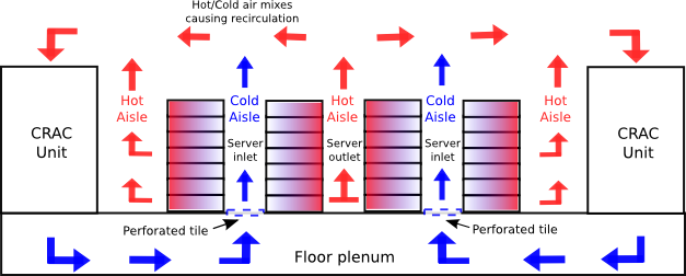
Figure 1: Typical raised-floor air-cooled Data Center layout

The maximum IT power density that can be deployed in the Data Center is limited by the perforated tile airflow. Because the plenum is usually obstructed (e.g. blocked with cables in some areas), a non-uniform airflow distribution is generated and each tile exhibits a different pressure drop. Moreover, in data centers where the hot and cold aisles are not isolated, which is the most common scenario, the heated exhaust air recirculates to the cold aisle, mixing with the cold air.

2.2 Temperature-energy tradeoffs

The factor limiting minimum data room cooling is maximum server CPU temperature. Temperatures higher than 85$\degree$C can cause permanent reliability failures [11]. At temperatures above 95$\degree$C, servers usually turn off to prevent thermal redlining. Previous work on server power and thermal modeling [12], shows how CPU temperature is dominated by: i) power consumption, which is dependent on workload execution, ii) fan speed, which changes the cooling capacity of the server, and iii) server cold air supply (inlet temperature).

Thus, to keep all the equipment under normal operation, CRAC units have to supply the air at an adequately low temperature to ensure that all CPU’s are below the critical threshold. However, inlet temperature is also not uniform across servers. The cold air temperature at the server inlet depends on several parameters: i) the CRAC cold air supply, ii) the airflow rate through the perforated tiles, and iii) the outlet temperature of adjacent servers due to air recirculation.

Setting the cooling air supply temperature to a low value, even though ensures safety operation, implies increased power consumption due to a larger burden on the chiller system. The goal of energy-efficient cooling strategies is to increase the cold air supply temperature without reaching thermal redlining. Due to the non-linear efficiency of cooling systems, lowering air supply temperature can yield important energy savings. A metric widely used is that each degree of increase in air supply temperature yields 4% energy savings in the cooling subsystem [13]. To increase air supply temperature safely, however, we need to predict not only the inlet temperature to the servers, but also the CPU temperature that each server attains under the current workload.

Due to the temperature gradients between hot and cold aisles and the data room layout and geometry, the air inside a data center behaves like a turbulent fluid. Thus, obtaining an analytical relation between cold air supply and server inlet temperature is not trivial, making inlet and CPU temperature prediction a challenging problem. Besides, data centers are composed of thousands of CPU cores, whose temperatures need to be modeled independently. This prevents the usage of classical regression techniques that need human interaction to train and validate the models.

3 Literature overview

Data center room thermal modeling enables both thermal emergency management and energy optimization, and enhances reliability. Because of the turbulent behavior of the air in the Data Center room, Computational Fluid Dynamics (CFD) simulation has traditionally been the most commonly used solution in both industry and academia [14].

CFD is used to model the inlet and outlet temperature of servers, given cold air supply parameters, room layout, server configuration and utilization, in order to either optimize cooling costs or detect hot spots [15]. CFD solvers perform a three-dimensional numerical analysis of the thermodynamic equations that govern the data room. Their main drawbacks is that they require and expert to configure the simulation, and are computationally costly both in the modeling stage (i.e. modeling a small-sized data room may take from hours to days) and in the evaluation phase, thus preventing their online usage. Moreover, CFD simulation is not robust to changes in the layout of the Data Center, i.e. server placement, open tiles, workload running or cold air supply setting.

To solve these issues, Chen et.al. [16] use CFD together with sensor information to calibrate the simulation and reduce computational complexity. Their work achieves a prediction error below 2$\degree$C when predicting temperature 10 minutes in advance. Other work [17] presents the Data Center as a distributed Cyber-Physical System (CPS) in which both computational and physical parameters can be measured with the goal of minimizing energy consumption. Our work leverages this concept by using a monitoring system [18] capable of collecting environmental (i.e. cold air supply and server inlet temperature, airflow, etc.) and server data (i.e. temperature, power, fan speed, etc.) from a real data center.

A common alternative to CFD are abstract heat flow models. These models characterize the steady state of hot air recirculation inside the data center. Recirculation is described by a cross-interference coefficient matrix which denotes how much of every node’s outlet heat contributes to the inlet of every other node. This matrix is obtained in an offline profiling stage using CFD [19]. Even though profiling is still costly, model evaluation can be performed online.

Machine learning techniques have also been used in Data Center modeling. The Weatherman [20] tool uses neural networks to predict the inlet temperature of servers, obtaining prediction errors below 1$\degree$C in over 90% of their traces. However, they use simulation traces obtained with CFD simulation for their training and test sets, instead of real data. The problem behind time series prediction can be explained as a problem of extracting a manageable set of adequate features, followed by a regression mechanism. Careful selection of features and their horizon is therefore of much greater importance compared with the static-data prediction problem. Neural network-based approaches require previous knowledge of the parameters that drive thermal modeling, obtaining them using pseudo-exhaustive algorithms. Our work, on the contrary, relies on the benefits of feature engineering in Symbolic Regression problems to obtain the relevant features and construct the models in an automated way.

The work by De Silva et al. [21] is the one most similar to ours, regarding the modeling methodology. The authors use Grammatical Evolution for electricity load prediction. As opposed to our work, this paper is focused on predicting the trend, momentum and volatility indicators of a timeseries, not on obtaining a physical model, i.e. they do not solve a multi-variable problem.

In summary, the main issues in all previous approaches are: i) they monitor and predict inlet temperature instead of CPU temperature, ii) modeling is performed for only certain hand-picked cooling and workload configurations, iii) the use of CPU utilization as a proxy for server power, iv) they assume data centers with homogeneous servers, v) server fan speed is considered constant, vi) results are not validated with real traces, and vii) model construction requires specific knowledge on the problem and classical feature selection, which prevents the usage of automated techniques.

Our work, on the contrary, first predicts inlet temperature and then uses this result to predict CPU temperature, which is the factor limiting cooling. Both in our training and test sets, we use real traces obtained from enterprise servers in a data center. Moreover, as shown in previous work [12], in highly multi-threaded enterprise servers, utilization is not a good proxy for power for arbitrary workloads.

Enterprise servers come with automatic temperature-driven variable fan control policies. When fan speed changes, so does the airflow and the server cooling capacity [22]. Our methodology also considers the contribution of variable fan speed, allowing us to predict temperature in heterogeneous data center setups running arbitrary workloads.

At the server level, Heather et al. [23] propose a server temperature prediction model based on simplified thermodynamic equations obtaining results within 1$\degree$C of accuracy. Even though this approach predicts CPU temperature and takes into account inlet temperature, it does not predict the inlet and needs specific knowledge about several server parameters. Our approach only uses data from the generic sensors deployed in the server and data room.

Another common approach to CPU temperature modeling is the usage of autoregressive moving average (ARMA) modeling to estimate future temperature accurately based on previous measurements [24]. Their main drawbacks are that, because they only use past temperature samples, the prediction horizon is usually below one second. Moreover, they do not provide a physical model, disregarding the effect of power or airflow, and need to be retrained often.

As opposed to others, our work achieves prediction horizons of 1 minute for CPU temperature and 10 minutes for inlet temperature with high accuracy. This enables data center operations to take action before thermal events occur, by changing either the workload or the cooling in the data center.

4 Gramatical evolution techniques

Evolutionary algorithms use the principles of evolution to turn one population of solutions into another, by means of selection, crossover and mutation. Among them, Genetic Programming (GP) has proven to be effective in a number of Symbolic Regression (SR) problems [25]. However, GP presents some limitations like bloating of the evolution (excessive growth of memory computer structures), often produced in the phenotype of the individual. In the last years, variants to GP like Grammatical Evolution (GE) appeared as a simpler optimization process [26]. GE is inspired in the biological process of generating a protein given the DNA of an organism. GE evolves computer programs given a set of rules, adopting a bio-inspired genotype-phenotype mapping process.

In this section, we describe how we perform feature selection, provide a brief insight on the grammars and mapping process, as well as on several model parameters.

4.1 Feature selection and model definition

In this work we use Feature Engineering (FE) and Grammatical Evolution to obtain a mathematical expression that models CPU and server inlet temperature. This expression is derived from experimental measurements in real server and data room scenarios, gathering data that have an impact on temperature, according to previous work in the area [12, 18]. To predict CPU temperature, we gather server power, fan speed, inlet temperature and previous CPU temperature measurements. For inlet temperature, we gather the CRAC air supply and return temperature, humidity, pressure difference through perforated tiles (which is a measurement that provides information about airflow) and previous inlet temperature measurements. Our goal is to predict temperature a certain time (samples) in advance, by using past data of the available magnitudes within a window. We may use past samples from the magnitude we need to predict, or even previously predicted data.

For illustration purposes, in Figure 2 we show a diagram in which CPU temperature is predicted 1 minute ahead given: i) 2 minutes of past measurements (data window) for fan speed, server power, inlet and CPU temperature and, ii) the previous CPU temperature predictions (prediction window).

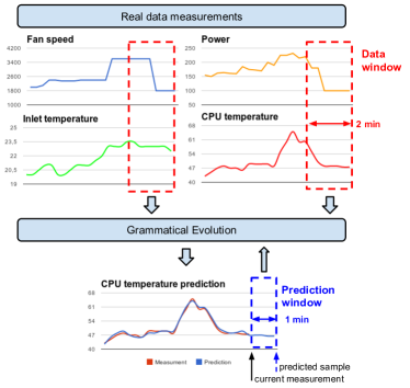
Figure 2: CPU temperature prediction diagram.

Formally, we claim that CPU temperature prediction for a certain time instant $\alpha$ samples into the future is a function of past data measurements within a window of size $i=\{0..W_{cpu}\}$, and previously predicted values within a window of size $j=\{1..\alpha\}$ as expressed in Eq.(1):

$$\begin{split}\widehat{T}_{CPU}(k+\alpha)=&f\big{(}T_{inlet}(k-i),FS(k-i),P(k-i),\\ &T_{CPU}(k-i),\widehat{T}_{CPU}(k+j)\big{)}\end{split}$$ (1)

where $T_{inlet}$ is a short form for the previous inlet temperature values in a window: $\{T_{inlet}(k-i)|i\in\{0,...,W_{cpu}\}\}$. $T_{CPU}$, $FS$ and $P$ are past CPU temperature, fan speed, and server power consumption values respectively, which are defined similarly, and $\widehat{T}_{CPU}$ are previous temperature predictions.

For inlet temperature, our claim is that inlet temperature $T_{inlet}$ of a certain server is driven by the room thermal dynamics and can be expressed as a function of the cold air supply (or return) temperature, $T_{CRAC}$, differential pressure across perforated tiles $\gamma$ (measured in inches of water, $inH_{2}O$) and data room humidity $h$ (in percentage), as in Eq.(2):

$$\begin{split}\widehat{T}_{inlet}(k+\beta)=&f\big{(}T_{CRAC}(k-i),\gamma(k-i),h(k-i),\\ &FS_{p-m}(k-i),\widehat{T}_{inlet}(k+j)\big{)}\end{split}$$ (2)

where the data window can be defined in the range $i=\{0..W_{inlet}\}$ and the prediction window is $j=\{1..\beta\}$

Note that, in general, $\alpha$ and $\beta$ are not equal, as the room dynamics are much slower than the CPU temperature dynamics of the servers, i.e. in a real data room we might need hours to appreciate substantial differences in ambient temperature, whereas CPU temperature changes within seconds. The selection of relevant features among all data measurements is a Symbolic Regression (SR) problem. In our approach, GE allows the generation of mathematical models applying SR.

Regarding both the structure and the internal operators, GE works like a classic Genetic Algorithm [27]. GE evolves a population formed by a set of individuals, each one constituted by a chromosome and a fitness value. In SR, the fitness value is usually a regression metric like Mean Squared Error (MSE). In GE, a chromosome is a string of integers. In the optimization process, GA operators, are iteratively applied to improve the fitness value of each individual. In order to compute the fitness function for every iteration and extract the mathematical expression given by an individual (phenotype), a mapping process is applied to the chromosome (genotype). This mapping process is achieved by defining a set of rules to obtain the mathematical expression, using grammars in Backus Naur Form (BNF) [26].

The process does not only perform parameter identification. In conjunction with a well-defined fitness function, the evolutionary algorithm is also computing mathematical expressions with the set of features that best fit the target system. Thus, GE is also defining the optimal set of features that derive into the most accurate power model.

Moreover, this methodology can be used to predict magnitudes with memory, such as temperature, where the current observation depends on past values. To incorporate time dependence, data used for model creation needs to be a timeseries. In addition, we need to tune our grammars so that they can produce models where past temperature values can be used to predict temperature a certain number of samples into the future. Grammar 1 shows an example where variable x may take values in the current time step $k$, i.e., $x[k-0]$ or in previous samples like $x[k-1]$ or $x[k-2]$. Moreover, a new variable $xpred[k-idx]$ can be included, that accounts for previously predicted values of variable $x$.

Including time dependence into a grammar has some drawbacks. First, we are substantially increasing the search space of our algorithms, as now the GE needs to search for the best solution among all variables within the specified window. As a consequence, the number of generations needed to obtain a good fitness value increases. Second, as we show in the results section, depending on the prediction horizon the models tend to fall into a local optimum, in which the best phenotype is the last available observation of the predicted variable. To address the latter challenge, we propose the use of the premature convergence prevention techniques that are next explained, and that also benefit the converge time of our algorithms. Despite the drawbacks, introducing time dependence in our modeling is a must, as temperature transients (both at the server and the data center level) are not negligible and need to be accurately predicted.

For a more detailed explanation on the principles of the mapping process, and how the BNF grammars are used to incorporate time dependence, the reader is referred to the Appendix.

¡expr¿ ::= ¡expr¿¡op¿¡expr¿ — ¡preop¿(¡expr¿) — ¡var¿

¡op¿ ::= +—-—*—/

¡preop¿ ::= sin— cos — log

¡var¿ ::= x[k-¡idx¿] — xpred[k-¡idx¿] — y — z — ¡num¿

¡num¿ ::= ¡dig¿.¡dig¿ — ¡dig¿

¡dig¿ ::= 0 — 1 — 2 — 3 — 4 — 5

¡idx¿ ::= 0 — 1 — 2

Grammar 1 Example of a grammar in BNF that generates phenotypes with time dependence

4.2 Preventing premature convergence

Premature convergence of a genetic algorithm arises when the chromosomes of some high rated individuals quickly dominate the population, reducing diversity, and constraining it to converge to a local optimum. Premature convergence is one of the major shortcomings when trying to model low variability magnitudes by using GE techniques.

To overcome the lack of variety in the population, work by Kureichick et al. [28] proposes the usage of Social Disaster Techniques (SDT). This technique is based on monitoring the population to find local optima, and apply an operator:

1. Packing: all individuals having the same fitness value except one are fully randomized.

2. Judgment day: only the fittest individual survives while the remaining are fully randomized.

Work by Rocha et al. [29] proposes the usage of Random Off-spring Generation (ROG) to prevent the crossover of two individuals with equal genotype, as this would result in the off-spring being equal to the parents. Individuals are tested before crossover and, if equal, then one off-spring (1-RO) or both of them (2-RO) are randomly generated.

Both previous solutions have shown important benefits in classical Genetic Algorithms problems. In our work, we use these techniques to improve the convergence time of our solutions, as we show in Section 6.

4.3 Fitness

The goal of using GE for data room thermal modeling is to obtain accurate models. Thus, our fitness function needs to express the error resulting in the estimation process. To measure the accuracy in our prediction, we would preferably use the Mean Absolute Error (MAE). However, because temperature is a magnitude that varies slowly and might remain constant during large time intervals, we need to give higher weight to large errors. To this end, the fitness function $f$ presented in Eq.(3) tries to reduce the variance of the model, leading the evolution to obtain solutions that minimize the the Root Mean Square Error (RMSE):

$$f=\sqrt{\frac{1}{N}\cdot\sum_{i}{e_{\mathrm{i}}}^{2}}$$ (3)

where the estimation error $e_{\mathrm{i}}$ represents the deviation between the real temperature samples (both for CPU and inlet temperature modeling) obtained by the monitoring system $T$, and the estimation obtained by the model $\widehat{T}$. $i$ represents each sample of the entire set of $N$ samples used to train the algorithms.

4.4 Problem constraints

As we are modeling the behavior of physical magnitudes for optimization purposes, we need to obtain a solution with physical meaning. To this end, we constrain the general problem of temperature modeling in several ways that are subsequently presented, while still being able to address heterogeneous workloads, architectures and topologies. In the results section we evaluate the impact of these constraints on the model generation stage.

4.4.1 Constraining the grammar

The mathematical expressions can be constrained to a limited number of functions with physical meaning. Because temperature exhibits exponential transients, we can include the exponential function in our grammar, whereas we do not find physical basis to include other mathematical functions such as sines or cosines.

4.4.2 Fitness biasing

Some parameters drive the variables being modeled. For instance, power consumption drives CPU temperature. As we want to obtain models able to capture the physical phenomena that drive temperature, this magnitude should be present in the final model. Thus, CPU temperature models that do not include power in their phenotype are expected to provide good results in the training phase, but to perform poorly for the test, as they are not capturing the physical phenomena. To solve this issue, we can force the appearance of some parameters by biasing the fitness, giving higher weights (i.e. worse fitness) to expressions that miss a parameter. By biasing fitness we speed-up convergence, we ensure that our models incorporate all parameters directly correlated with temperature, but we could obtain less accurate results.

4.4.3 Real vs. mixed models

Purely real models only use real temperature data measurements to predict future samples. Purely predictive models do not used previous temperature measurements, but may use previous predictions. Mixed models may used both real and predicted data. Adding the predicted samples as a variable increases the size of the search space but may provide higher accuracy.

5 Experimental Methodology

In this section we describe the experimental methodology followed in this paper to model server and environmental parameters in Data Centers. First, we describe an scenario consisting only in the temperature prediction of one server in a small air-cooled data room. We use this scenario to tune the model parameters, testing those that generate better models and studying the convergence of the solutions. Then, we apply the best algorithm configuration to a real data center. As a case study, we use real traces of CeSViMa Data Center, a High Performance Computing cluster at Universidad Politécnica de Madrid in Spain.

5.1 Reduced scenario

This scenario consists on an Intel Xeon RX-300 S6 server equipped with 1 quad-core CPU and 16GB of RAM. The server is installed in a rack with another 4 servers, 2 switches and 2 UPS units, in an air-cooled data room of approximately 30$m^{2}$, with the rack inlet facing the cold air supply and the outlet to the heat exhaust. The cooling infrastructure consists on a Daikin FTXS30 split that pumps cold air from the ceiling, and there is no floor plenum. The cold air supply ranges from 16$\degree$C to 26$\degree$C. The data room is fully monitored, and both the cooling and server workload are controllable.

5.1.1 Monitoring

Both the server and data room are fully monitored using the internal server sensors and a wireless sensor network, as described in [18]. In particular, server CPU temperature and fan speed values are obtained via the server internal sensors, collected through the Intelligent Platform Management Interface (IPMI) tool . IPMI allows polling the internal sensors of enterprise servers with negligible overhead. As the server is not shipped with power consumption sensors, we use non-intrusive current clamps connected to the power cord of the server to gather total server power consumption. Wireless sensors monitor the inlet temperature of the server, the cold air supply temperature of the split unit and data room humidity. Data are sent to the monitoring server, stored and aligned to ensure a common timestamp.

5.1.2 Training and test set generation

We generate the training and test set by assigning a wide variety of workloads that exhibit various stress levels in the CPU and memory subsystems of the server while we modify the cold air supply temperature of the split in a range from 16$\degree$C to 26$\degree$C. All workloads used are a representative set, in terms of stress to the server subsystem and power consumption, of the ones that can be found in High-Performance Computing data centers. Also, the temperatures selected for cold air supply temperature are within the allowable ranges in current data centers.

The workloads used are the following: i) Lookbusy, a synthetic workload that stresses the CPU to a customizable utilization value, avoiding the stress of memory and disk; ii) a modified version of the synthetic benchmark RandMem, that allows us to stress random memory regions of a given size with a given access pattern, and iii) HPC workloads belonging to the SPEC CPU 2006 benchmark suite [30].

During training, we launch Lookbusy and Randmem at various utilization values, plus a subset of the SPEC CPU 2006 benchmarks that exhibit a distinctive set of characteristics according to Phansalkar et al. [31]. Both the arrival time and task duration are randomly selected. During execution, the cold air supply temperature is also randomly changed. For the test set, we randomly launch a SPEC CPU benchmark, with random waiting intervals while changing cold air supply temperature.

Our monitoring system collects all data with a 10 second sampling interval for a total time of 5 hours for the training and 10 hours for the test set. Figure 3 shows part of the training set used for modeling.

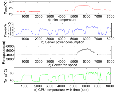
Figure 3: Training samples used for CPU temperature modeling

5.2 Case study: CeSViMa Data Center

To show how our solution can be applied to a real data center scenario, this paper presents a case study for a real High-Performance Computing Data Center at the Madrid Supercomputing and Visualization Center (CeSViMa). CeSViMa hosts the Magerit Supercomputer, a cluster consisting of 286 computer nodes in 11 racks, providing 4,160 processors to execute High-Performance jobs on demand. 245 of the 286 nodes are IBM PS702 2S with 2 Power7 CPU’s blade servers, each with 8 cores running at 3.3GHz and 32GB of RAM. The other 41 nodes are HS22 2U servers with 2 Intel Xeon processors of 8 cores each at 2.5GHz and 64GB RAM.

CeSViMa data room has a cold-hot aisle layout and is cooled by means of 6 CRAC units arranged in the walls that impulse air through the floor plenum. To control data room cooling, the air return temperature of each CRAC unit can be set independently. The room has a total size of 190 square meters. Figure 4a shows the layout of the data center. Rack 0 is a control rack that runs no HPC computation. Racks 1-9 are filled with Power7 blade servers, whereas rack 10 contains Intel Xeon servers. Each Power7 node is installed in a blade center. Each blade center contains up to 7 blades, and each rack contains 4 chassis (C01 to C04), as shown in Figure 4b. To run our models, we have deployed the same sensor network as in the reduced scenario. In particular, to model inlet temperature we gather inlet temperature, humidity, CRAC air return temperature and differential pressure through the floor plenum. Because we have placed pressure sensors in the tiles in front of racks 1 and 4, we model the Power7 nodes in these racks. To model CPU temperature, we also collect CPU temperature and fan speed of all servers via IPMI. CeSViMa Power7 chassis do not have per-server power sensors and we are not able to deploy current clamps. Thus, we use per-server utilization as a proxy for the power consumption of the node. As stated before, utilization is not an accurate metric for arbitrary workloads. However, because of the nature of the workloads in CeSViMa and only for thermal modeling purposes, utilization can be used as a proxy variable to power consumption, as we show in Section 6.

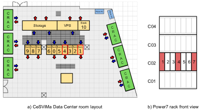
Figure 4: CeSViMa data room layout. Models are developed for Power7 nodes 1,4 and 7 at high c02 in racks 1 and 4.

In this work we show the modeling results for the servers highlighted in red in Figure 4, i.e. nodes 1,4,7 at chassis c02 of both rack 1 and 4. These nodes are the ones that exhibit the most variable workload and extreme temperature conditions and constitute the worst-case scenario for modeling.

5.3 Modeling framework

Because of the large number of servers in CeSViMa, to enable cooling optimization we need a framework that allows to automatically model and predict the CPU and inlet temperature of all servers. Even though CeSViMa is a small-sized data room, it has a very high density in terms of IT equipment. For instance, the amount of data gathered that needs to be processed to enable full environmental modeling and prediction, for a period of 1 year, is above 100GB. Thus, modeling the whole data center with traditional approaches that require human interaction is not feasible.

Our work uses the proposed GE techniques to automatically model all the parameters involved in data center optimization by automatically running the training of the algorithms and testing them during runtime.

6 Results

In this section we present the experimental results obtained when applying Grammatical Evolution to model CPU and inlet temperature. First, we show the results for the controlled scenario, describing the best algorithm configuration, and compare our method with state-of-the art solutions. Then, we apply the best configuration to train and test the models in a real data center scenario.

6.1 Algorithm setup and performance

First, we use GE to obtain a set of candidate solutions with low error when compared to the temperature measurements in our controlled experimental setup, under different constraints.

After evaluating the performance of our model with several setups, we select the following one for each model in this paper:

• Population size: 200 individuals

• Chromosome length: 100 codons

• Mutation probability: inversely proportional to the number of rules.

• Crossover probability: 0.9

• Maximum wraps: 3

• Codon size: 8 bits (values from 0 to 255)

• Tournament size: 2 (binary)

For CPU temperature prediction, we use a data window of $W_{cpu}=20$ samples (corresponding to 200 seconds) and a prediction window of $\alpha=6$ (corresponding to 60 seconds). The data window is heuristically chosen with respect to the largest observed temperature transient, and its size is a trade-off between model accuracy and convergence time. In this sense, the data window needs to incorporate enough samples to capture the trends of thermal transients, but we also need to consider that the larger the data window, the larger the exploration space. The prediction window needs to be selected with respect to the time it takes to actuate on the system and observe a response. In our case, the data window size $W_{cpu}$ has been chosen in accordance to our previous work on server power modeling, where we analytically modeled temperature transients in enterprise servers, observing that the largest transients, i.e. the worst-case modeling scenario, occur for the lower fan speed values [12]. The prediction window is chosen given the physical constraints of the problem: 1-minute prediction is sufficient time to change the workload assignment of a server, as canceling the workload of a server in case of thermal redlining takes few seconds.

For inlet temperature prediction, we also use a data window of $W_{inlet}=20$ samples but a prediction window of $\beta=5$ samples. Inlet temperature dynamics are much slower than CPU temperature. Because of this, a sampling rate of 2 minutes over inlet temperature is sufficient to get accurate results. Given the size of the prediction window, we are able to obtain inlet temperature samples 10 minutes advance, which is sufficient time to act upon data room cooling.

Next, we present the comparison among several configurations in terms of grammar expressions and rules, premature convergence prevention and fitness biasing. We detail our results for CPU temperature modeling. The procedure to tune inlet temperature models is completely equivalent.

6.1.1 Data preprocessing and model simplification

Because the power measurements of the Intel Xeon server are taken with a current clamp, the power values obtained exhibit some noise. We preprocess the data to eliminate high-frequency noise, smoothing the power consumption trace by means of a low pass filter. The remaining traces did not exhibit noise, so no preprocessing was needed.

Moreover, we perform variable standardization for every feature (in the range $[1,2]$) to assure the same probability of appearance for all the variables and to enhance the GE symbolic regression.

6.1.2 Grammars used

To model CPU temperature we have tested three different grammars:

• The first is shown in Grammar 2 and contains a wide set of operands and preoperands (rules II and III), that do not necessarily yield models with a physical meaning.

• The second grammar is a variation of Grammar 2 in which the number of preoperands (rule III) is reduced to exponentials only, i.e. $\synt{preop}::=exp$

• The last grammar is the one presented in Grammar 3 and also reduces the set of possible expressions (rule I).

¡expr¿ ::= ¡expr¿¡op¿¡expr¿—(¡expr¿¡op¿¡expr¿)
— ¡preop¿(¡expr¿)—¡var¿—¡cte¿

¡op¿ ::= +—-—*—/

¡preop¿ ::= exp — sin — cos — tan

¡var¿ ::= TS[k-¡idx¿]—TIN[k-¡idx¿]—PS[k-¡idx¿]
—FS[k-¡idx¿]

¡idx¿ ::= ¡dgt2¿¡dgt¿

¡cte¿ ::= ¡dgt¿.¡dgt¿

¡dgt¿ ::= 0—1—2—3—4—5—6—7—8—9

¡dgt2¿ ::= 0—1

Grammar 2 Grammar used for CPU temperature modeling in BNF, that uses inlet temperature (TIN), fan speed (FS), power consumption (PS), past CPU temperature (TS) and past predicted CPU temperature (TpS)

From the previous three grammars the one that has faster convergence time to achieve a low error, is Grammar 3. Constraining the grammar improves convergence time and provides phenotypes that have physical meaning, without an increase in the modeling error obtained. Thus, for the remaining of the paper we work with the simplified Grammar 3 when modeling CPU temperature.

¡expr¿ ::= ¡expr¿¡op¿¡expr¿—(¡expr¿¡op¿¡expr¿)
¡preop¿(¡exponent¿)—¡var¿—¡cte¿

¡op¿ ::= +—-—*—/

¡preop¿ ::= exp

¡exponent¿ ::= ¡sign¿¡cte¿*¡var¿
—¡sign¿¡cte¿*(¡var¿¡op¿¡var¿)

¡sign¿ ::= +—-

¡var¿ ::= TpS[k-¡idx¿]—TS[k-¡idx¿]—TIN[k-¡idx¿]
—PS[k-¡idx¿]—FS[k-¡idx¿]

¡idx¿ ::= ¡dgt¿

¡cte¿ ::= ¡dgt2¿.¡dgt2¿

¡dgt¿ ::= 1—2—3—4—5—6—7—8—9—10—11—12—13—14
—15—16—17—18—19—20

¡dgt2¿ ::= 0—1—2—3—4—5—6—7—8—9

Grammar 3 Simplified grammar in BNF format used for CPU temperature modeling

We test two variations of this grammar: i) one that searches for a mixed model (i.e. uses past temperature predictions, and it is the one shown in Grammar 3), and ii) the one that provides a real model (i.e. only uses CPU temperature measurements). The only difference between the mixed and the real grammars, is the presence of the parameter $TpS$.

6.1.3 Tested configurations

With respect to premature convergence, we test three different techniques:

• No premature convergence technique applied

• Random Off-Spring Generation (2-RO) plus Packing, keeping no more that a 5% of equal individuals.

• Random Off-Spring Generation (2-RO) plus Packing, leaving no more than 1 individual with equal phenotype.

For each of the previous configurations, we run both real and mixed models, with the goal of comparing the convergence time and the fitness evolution of each configuration. Because of the random evolution of the algorithms, for comparison purposes, we run the same model training 5 times and average the RMSE obtained for different number of generations. Figure 5 shows the RMSE evolution for the three configurations, with both real and mixed models.

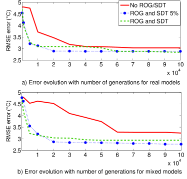
Figure 5: CPU temperature error evolution for real and mixed models under different premature convergence prevention techniques: i) no technique applied, ii) ROG + SDT keeping 5% of equal individuals and iii) ROG + SDT randomizing all equal individuals.

When we do not apply any technique, error decay is much slower, as population loses diversity and improves only due to mutation in the individuals. The impact is higher for the mixed models, where search space is larger. When we apply ROG and SDT, we need less generations to obtain good fitness values. However, keeping only 1 individual with the same phenotype and randomizing the remaining population is too aggressive, while keeping a higher percentage of equal individuals, i.e. a 5%, yields better results. As shown, using 30,000 generations is enough to obtain low RMSE values.

Regarding fitness biasing, Figure 6 shows the differences in terms of RMSE for different number of generations for real and mixed models when we bias the fitness to force all parameters and when we do not bias it. Convergence is similar, being slightly better that of the non-biased models. In fact, all variables in the grammar tend to appear in non-biased models, backing up the hypothesis that all those magnitudes are correlated with temperature.

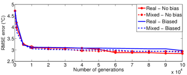
Figure 6: CPU temperature error evolution for real and mixed models under ROG + SDT 5% when fitness is biased vs. not biased.

Finally, we show results for both the training and test set when modeling CPU temperature with the best configuration, i.e. a mixed model obtained with Grammar 3, using ROG and Packing techniques leaving 5% of equal individuals, and not biasing the fitness. Table 1 shows the 5 better phenotypes obtained and their corresponding RMSE and MAE values for the test set after simplification. To avoid overfitting, we use the five best models to compute the samples of the test set, i.e., we predict the next temperature sample with all five equations, obtaining 5 different results, and we average them to obtain the prediction value. By applying this methodology we obtain a RMSE of 2.48$\degree$C and a MAE of 1.77$\degree$C. Because CPU temperature sensors usually have a resolution of 1$\degree$C we consider these results to be accurate enough for our purposes. Figure 7 shows a zoom-in of the real CPU temperature trace and its prediction, for both the training and the test set. As can be seen, the prediction accurately matches the measured values in both the training and test sets.

Phenotype	RMSE	MAE
$TS[k-3]+PS[k-1]-PS[k-4]+1.1\cdot TIN[k-7]/(e^{(-0.1\cdot(TpS[k-8]-TS[k-3]))}$
$\cdot(PS[k-20]/9.9)+9.9)-(e^{(-4.5\cdot(TpS[k-5]/TS[k-19]))}\cdot TS[k-7])-9.6$	2.8	2.08
$TS[k-5]+PS[k-1])-PS[k-5]+(TS[k-5]/5.7-e^{(-1.3\cdot(TS[k-5]/TIN[k-12]))}\cdot TS[k-5])$
$+PS[k-11]/(3.7-TS[k-5]\cdot(e^{(-0.3\cdot(PS[k-18]+FS[k-7]))}-e^{(-4.9\cdot(PS[k-12]/PS[k-16]))}))-9.8$	2.59	1.86
$TS[k-5]+PS[k-1]-PS[k-4]+e^{(+6.1\cdot(TIN[k-10]/TS[k-5]))}-5.2)-TIN[k-14]\cdot(0.06\cdot(TIN[k-7]/TS[k-5]))$
$+(PS[k-1]/3.1\cdot TIN[k-7])\cdot TS[k-5]-(PS[k-20]/TIN[k-7])\cdot^{(-6.4\cdot(TIN[k-15]/TS[k-11]))}-8.0$	2.77	2.01
$TS[k-3]+PS[k-1]-PS[k-4]-e^{(-4.1\cdot(TpS[k-5]/TIN[k-19]))}/TS[k-3]$
$+(TpS[k-1]/(e^{(-0.1\cdot(TpS[k-8]-TS[k-3]))}\cdot(PS[k-20]/9.9)+9.2))/1.6-9.6$	2.55	1.77
$TS[k-1]+0.73\cdot(PS[k-1]\cdot 4.4-PS[k-2]\cdot 4.4-TS[k-1]+TpS[k-8]+e^{(-0.2\cdot TIN[k-8])}$
$+(e^{(-3.4\cdot(PS[k-20]/PS[k-10]))}-e^{(-4.0\cdot(PS[k-6]/PS[k-19]))})\cdot TpS[k-12]/9.0-0.9)$	2.5	1.75

Table 1: Phenotype, RMSE and MAE for the test set in the CPU temperature modeling reduced scenario

(a) 1-minute training set prediction for mixed model

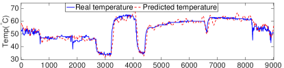
(b) 1-minute test set prediction for mixed model

Figure 7: Training and test set CPU temperature prediction vs. real measurements with time (secs)

6.2 Comparison to other approaches

We compare our results with three common techniques for CPU temperature modeling in the state-of-the-art: autoregressive moving average models, linear subspace identification techniques and dynamic neural networks. We first briefly describe these three modeling techniques and then we show the results obtained and compare them with our proposed technique.

6.2.1 ARMA models

ARMA models are mathematical models of autocorrelation in a time series, that use past values alone to forecast future values of a magnitude. ARMA models assume the underlying model as stationary and that there is a serial correlation with the data, something that temperature modeling accomplishes. In a general way, an ARMA model can be described as in Equation 4:

$$y_{t}=\sum_{i=1}^{p}(a_{i}\cdot y_{t-i})=e_{t}+\sum_{j=1}^{q}(c_{j}\cdot e_{t-j})$$ (4)

where $y_{t}$ is the value of the time series (CPU temperature in our case) at time $t$, $a_{i}$’s are the lag-i autoregressive coefficients, $c_{i}$’s are the moving average coefficient and $e_{t}$ is the error. The error is assumed to be random and normally distributed. $p$ and $q$ are the orders of the autoregressive (AR) and the moving average (MA) parts of the model, respectively.

The ARMA modeling methodology consists on two different steps: i) identification and ii) estimation. In our work we use an automated methodology similar to the one proposed by Coskun et.al. [24]. During the identification phase, the model order is computed, i.e, we find the optimum values for $p$ and $q$ of the $ARMA(p,q)$ process. To perform model identification we use an automated strategy, that computes the goodness of fit for a range of $p$ and $q$ values, starting by the simplest model (i.e., an ARMA(1,0)). The goodness of fit is computed using the Final Prediction Error (FPE), and the best model is the one with lowest FPE value, given by Equation 5:

$$FPE=\frac{1+n/N}{1-n/N}\cdot V$$ (5)

where $n=p+q$, $N$ is the length of the time series and $V$ is the variance of the model residuals. For a fair comparison with our proposed methodology, the model obtained needs to forecast $\alpha=6$ samples.

6.2.2 N4SID

N4SID is a subspace identification method that estimates an $n$ order state-space model using measured input-output data, to obtain a model that represents the following system:

$$\dot{x}(t)=Ax(t)+Bu(t)+Ke(t)$$ (6)

$$y(t)=Cx(t)+Du(t)+e(t)$$ (7)

where $A$,$B$,$C$ and $D$ are state-space matrices, $K$ is the disturbance matrix, $u(t)$ is the input, $y(t)$ is the output, $x(t)$ is the vector of $n$ states and $e(t)$ is the disturbance.

State-space models are models that use state variable observations to describe a system by a set of first-order differential equations, using a black-box approach. The approach consists on identifying a parameterization of the model, and then determining the parameters so that the measurements explain the model in the most accurate possible way. They have been very successful for the identification of linear multivariable dynamic systems.

To be constructed, certain parameters need to be fed into the model, such as the number of forward predictions ($r$), the number of past inputs ($s_{u}$), and the number of past outputs($s_{y}$). Again, for a fair comparison with our proposed methodology, we need a model in the form $N4SID[r,s_{u},s_{y}]$ where $r=6,s_{u}=20$ and $s_{y}=20$.

6.2.3 NARX

A Nonlinear Autoregressive eXogenous (NARX) model is a nonlinear autoregressive model with exogenous inputs. In this case, the current value of a time series is computed in function of a) past values of the same series, and b) current and past values of the exogenous series. Additionally, the model contains an error term, since knowledge of the other terms will not enable the current value of the time series to be predicted with precision. This is model is described as follows:

$$y(t)=F(y(t-1).y(t-2),y(t-3),\ldots,u(t),u(t-1),u(t-2),u(t-3),\ldots)+e(t)$$ (8)

where $y(t)$ is the output, $u(t)$ is the exogenous variable and $e(t)$ is the error term. $F$ is a nonlinear function, and in our case is defined through a neural network. The NARX model is based on the linear ARX model, which is commonly used in time-series modeling.

6.2.4 Model comparison

Finally, we compare the results for CPU temperature modeling between our proposed approach, ARMA, N4SID, and NARX models, all of them with a prediction window of 6 samples (1 minute). To perform a statistical comparison, we have conducted a non-exhaustive 5-fold cross-validation. The complete data set is obtained from more than 10 hours of temperature traces gathered from an Intel Xeon RX-300 S6 server running a wide range of workloads under various cooling setups. This data set has been partitioned into 5 equal sized subsamples. A single subsample is retained as the validation data for testing the model, and the remaining 4 subsets are used as training data. This process is repeated 5 times with each of the 5 subsamples used exactly once as the validation data. RMSE and MAE are averaged to perform a comparison between ARMA, N4SID, NARX and GE. Each resultant set of five models will be averaged to produce the final estimation.

Model	Training set		Test set
	RMSE	MAE	RMSE	MAE
ARMA1,4	$3.38\pm 0.23$	$1.62\pm 0.13$	$3.23\pm 1.02$	$1.62\pm 0.57$
ARMA9,8	$3.35\pm 0.24$	$1.70\pm 0.14$	$3.24\pm 1.01$	$1.74\pm 0.64$
N4SID	$2.55\pm 0.28$	$1.69\pm 0.07$	$3.98\pm 1.11$	$2.93\pm 0.58$
NARX	$2.53\pm 0.10$	$1.64\pm 0.05$	$3.88\pm 1.16$	$2.35\pm 0.69$
GE	$2.32\pm 0.19$	$1.50\pm 0.08$	$2.56\pm 0.90$	$1.66\pm 0.45$

Table 2: RMSE and MAE in CPU temperature prediction for each model (ARMA, N4SID, NARX and GE)

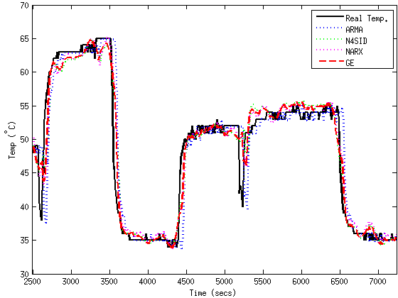
Figure 8: Zoomed-in averaged CPU temperature modeling comparison between ARMA(1,4), N4SID, NARX and GE

Table 2 shows the RMSE and MAE errors obtained for our proposed modeling technique based on GE, ARMA, N4SID and NARX models, and Figure 8 shows a zoom-in into the CPU temperature curve for the actual measurements and the averaged prediction of the five models obtained in the cross validation over the whole data set. As can be seen, GE models are the ones with both lower RMSE and MAE. Moreover, the CPU temperature trend is accurately predicted. This does not happen for ARMA models that, even though keep the maximum error low, provide values that are always behind the real trend, yielding poor forecasting capabilities. This issue cannot be solved by increasing the model order, as shown in Table 2. N4SID models, even though they are very accurate in the training set, perform poorly in the test set and have an important bias error. Even if the bias error is corrected (which has been done in Figure 8) the prediction is still behind the measurements and the model is unable to capture the system dynamics. NARX models clearly show an overfitting effect in the training data. The GE prediction, even though has more oscillations (due to the smoothed noise of the power consumption signal) is the only one that captures the temperature trend, advancing the real measurements.

6.3 Inlet temperature modeling

For inlet temperature modeling we perform the same study than for CPU temperature in terms of grammars, premature convergence and fitness biasing. As expected, the results in terms of the best model configuration yield very similar results. Thus, for inlet temperature modeling, we use the same configuration: i) a mixed model using a simplified version of the grammar that only allows exponentials, ii) SDT with 5% packing and iii) RMSE fitness function without biasing.

The BNF grammar used is very similar to Grammar 3, where instead of rule VI, we use the following rule:

¡var¿ ::= TIN[k-¡idx¿] — TpIN[k-¡idx¿] $\alt$ TSUP[k-¡idx¿] — HUM[k-¡idx¿]

where TSUP is cold air supply temperature, HUM is humidity, TIN are past inlet temperatures and TpIN are past inlet temperature predictions. Figure 9 shows the prediction for the test set. The RMSE of the prediction is of 0.33$\degree$C and MAE is 0.27$\degree$C for a prediction window of 10 minutes and for the test set. Again, the model includes all the available variables, i.e., TSUP, TIN and HUM appear in the final model.

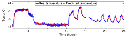
Figure 9: 10-minute inlet temperature prediction in the reduced scenario for a mixed model with SDT Packing 5% and simplified grammar

6.4 Data Center modeling

We use the previous model with the same configuration to predict the CPU and inlet temperature of the blade servers at CeSViMa data center. Because CeSViMa is a production environment, when it comes to server data, we are subject to the data sampling rates provided by the data center. CeSViMa collects all data from servers every 2 minutes, and environmental data (i.e. from coolers) every 15 minutes. Thus, for both CPU and inlet temperatures, we need to change our prediction windows. For CPU temperature we use a prediction window $\alpha^{\prime}=1$, which means that we predict CPU temperature two minutes into the future. For inlet temperature we use a prediction window $\beta^{\prime}=1$ samples, i.e. we predict temperature 15 minutes ahead.

Because in CeSViMa we cannot control the workload being executed, nor modify the cooling setup, we need to select longer training and tests sets to ensure that they exhibit high variability on the magnitudes of interest. For CPU temperature, we select 2 days of execution for the training set, and 4 days for the test set. For inlet temperature, which varies very slowly in a real data center setup we use 14 days of execution for both the training and the test set.

Figure 10 shows a zoomed-in plot of the measured and predicted inlet temperature to the chassis c02 of racks 1 and 4 in CeSViMa data center for a period of 8 days. Figure 11 shows the measured and predicted CPU temperature traces for blades b01, b04 and b07 in chassis c02 of both racks, for the first two days of the same period, as well as the prediction error (i.e. the difference between the real measurements and the prediction). To generate these last models, instead of using the real inlet temperature measurements, we use predicted inlet temperature. This way, we are able to accurately predict all variables needed for optimization.

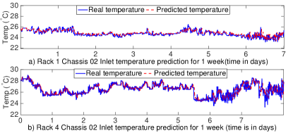
Figure 10: Inlet temperature modeling for various racks

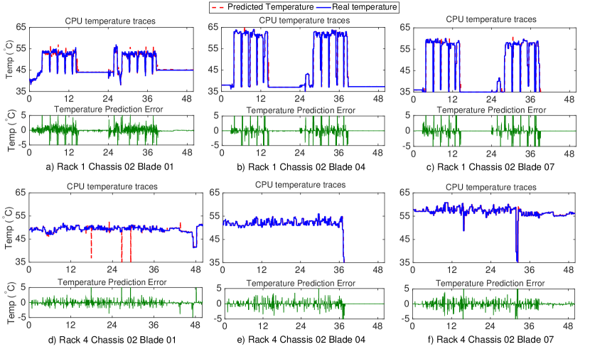
Figure 11: Data Center CPU temperature modeling and prediction error for various servers in different racks for 2 days of traces (time in hours)

Model	Phenotype	Train.	Test
Inlet	$TIN[k-1]+e^{(-4.3\cdot(TRET2[k-3]/TRET2[k-11]))}/TIN[k-1]\cdot(e^{(+1.5\cdot TIN[k-5])}$	0.32	0.4
Rack1	$-e^{(-3.8*(PDIF[k-20]-TIN[k-1]))})$
Inlet	$TIN[k-1]+3.1/e^{(+5.0\cdot TIN[k-1])}\cdot e^{(+2.2\cdot TIN[k-2])}-e^{(-2.9\cdot TpIN[k-3])}\cdot TRET3[k-12]\cdot$
Rack4	$(TRET3[k-5]+e^{(-4.9\cdot(HUM[k-6]/TRET2[k-1]))}/TIN[k-2]/e^{(+7.2\cdot(PDIF[k-20]-TIN[k-1]))})$	0.18	0.44
CPU	$TS[k-1]+(PS[k-20]\cdot FS[k-1]-9.4\cdot(TpS[k-5]\cdot TpS[k-2]))/(e^{(+2.0\cdot FS[k-7])}/$
Rack1, C02, B01	$e^{(-4.1\cdot TpS[k-5])}/(2.3+e^{(+1.7*(TpS[k-10]*TpS[k-10]))}+e^{(+1.5*FS[k-1])}-e^{(+1.6*PS[k-7])}))$	0.68	0.76
CPU	$TS[k-1]+e^{(-7.2*(TS[k-6]/PS[k-1]))}/(e^{(-6.1*(TS[k-10]-PS[k-15]))}/5.6/FS[k-20]$
Rack1, C02, B04	$-1.7+TpS[k-20]-e^{(-3.0*(TIN[k-4]/TS[k-15]))})$
CPU	$TS[k-1]+e^{(-6.2\cdot(TS[k-2]\cdot TIN[k-11]))}/((e^{(-9.8\cdot TS[k-8])}+e^{(-5.2*(TS[k-9]*PS[k-19]))})$	0.51	0.85
Rack1, C02, B07	$\cdot e^{(+5.8*FS[k-9])})$
CPU	$TS[k-1]+e^{(-3.1\cdot TS[k-2])}/(((TS[k-3]/PS[k-3])+(FS[k-18]-FS[k-8])/$	0.55	0.75
Rack4, C02, B01	$e^{(-9.4\cdot(FS[k-1]-TpS[k-9]))})-TpS[k-4]+(TpS[k-6]+TS[k-3])-(TIN[k-3]/TpS[k-9]))$	0.29	0.46
CPU
Rack4, C02, B04	$TS[k-1]+e^{(-5.7\cdot(TpS[k-6]*TpS[k-10]))}/e^{(+9.9\cdot(TpS[k-9]-TIN[k-10]))}$	0.26	0.73
CPU
Rack4, C02, B07	$TS[k-1]+TIN[k-11]\cdot e^{(-9.5\cdot(TpS[k-10]/TIN[k-5]))}/e^{(-9.9\cdot(TIN[k-10]-TS[k-5]))}$	0.43	0.87

Table 3: Phenotype and average error (in Celsius) in training and test set for CPU and inlet temperature modeling in a production Data Center

Table 3 shows the phenotypes obtained for CPU and temperature modeling of the servers in CeSViMa data center. We also report MAE for both training and test sets. We observe that all phenotypes that model CPU temperature incorporate the parameters of interest (inlet temperature, power and fan speed), and we obtain errors below 1$\degree$C in all cases. The average RMSE across models are 1.52 $\degree$C and 1.57$\degree$C for the training and test set respectively. As for inlet temperature, the phenotypes incorporate both differential pressure, and CRAC return temperature. Moreover, depending on the rack placement, the influence of the CRAC units vary. Here we can observe the benefits of the feature selection performed by GE. Rack1, which is the leftmost rack in the data center, is affected only by CRAC2; whereas Rack4, situated in the middle of the row, is affected both by CRAC2 and CRAC3. The model automatically incorporates the most relevant features, discarding the irrelevant ones. For inlet temperature prediction, our error is below 0.5$\degree$C, which is enough for our purposes and below other state-of-the-art approaches.

7 Discussion

In this section we briefly discuss the applicability of our models, and the computational effort needed to model a full data center scenario, to validate the feasibility of our approach.

7.1 Applicability

The goal of our modeling is predicting server CPU temperature under variable cooling setups, so that cooling-associated costs can be reduced without incurring on reliability issues. To this end, we first predict the inlet temperature of servers given the data room conditions and cooling setup, and use this result to predict server temperature.

Having analyzed the spatio-temporal variability of inlet temperature traces in CeSViMa data center, we find that it is sufficient to predict inlet temperature at 3 different heights (at the bottom, middle and top of the rack), in one out of two racks. This way, we need to generate 30 inlet temperature models at most. Because the maximum CPU temperature in the data center is the one limiting the cooling, at most we need to predict the CPU temperature of each server in the data room, i.e. we need as many models as servers in the data center. However, if by analyzing the traces we find that there is a subset of CPUs that limit the maximum cooling of the overall data center, our problem can be reduced to modeling those that always exhibit higher temperatures. For the particular case of the traces of CeSViMa, if we examine 6 months of CPU temperature traces, we find that the CPUs limiting the cooling are the blades b04 and b07 placed in the second chassis (c02) of all racks. In this sense, for energy optimization purposes our problem reduces to generating 10 different models. These models allow us to predict the maximum server temperature attained in the data center and, thus, detect any potential thermal redlining and act before it occurs. Moreover, to leverage energy optimization, our results can be used to set cooling dynamically during runtime, by predicting the maximum data center CPU temperature under various cooling conditions and increasing CRAC air supply temperature without incurring in reliability issues.

Even though in this paper we have applied our modeling methodology to a raised-floor air-cooled data center scenario, the proposed technique is also valid for data centers equipped with other state-of-the-art cooling mechanisms, such as in-row or in-rack cooling used in high-density racks.

7.2 Computational effort

Our approach is computationally intensive in the model training stage. The GE model needs to evolve a random initial population for 30,000 generations to obtain accurate results. In our experiments, running 30,000 generations of 4 different models in parallel takes 28h in a computer equipped with a QuadCore Intel i7 CPU @3.4GHz and 8GB of RAM. This computational cost is much larger than the computational cost for training ARMA and N4SID models. However, to obtain accurate results ARMA needs to be manually tuned, and N4SID requires a manual feature selection step that greatly impacts accuracy, whereas GE models can be automatically developed.

However, as the models obtained for homogeneous servers are very similar, it is possible to reduce the training overhead by using already evolved populations to fine-tune the models instead of using the a new random population every time. This way, we can reduce the training time significantly.

As for the model testing, in the worst case scenario, the model needs to be tested every 10 seconds. The overhead to test one model is found to be negligible. In this sense, it is feasible to compute all temperatures to find the maximum. Moreover, because of the temperature imbalances of servers in the data room we can reduce the amount of models run to those that are limiting the cooling, i.e. the servers with higher CPU temperature values. Overhead incurred by testing is in the same order of magnitude than the overhead of ARMA and N4SID, but provides better results in terms of error.

8 Conclusions

In this paper we have presented a methodology for the unsupervised generation of models to predict on runtime the thermal behavior of production data centers running arbitrary workloads and equipped with heterogeneous servers.

Our approach leverages the usage of Grammatical Evolution to automatically generate models of the data room by using real data center traces. Our solution allows to predict the CPU temperature and inlet temperature of servers, with an average error below 2$\degree$C and 0.5$\degree$C respectively. These errors are within the margin obtained by other off-line supervised approaches in the state-of-the art. Our solution, generates the models in an unsupervised way, is able to work on runtime, is trained and tested in a real scenario, and does not require the usage of CFD software.

To the best of our knowledge our work is the first to propose data center temperature forecasting using evolutionary techniques, allowing predictive model generation for runtime optimization.

Appendix

In this Appendix we provide further information on the mapping process used by our grammar. For a more detailed explanation on the principles of GE, the reader is referred to [32]. A BNF specification is a set of derivation rules, expressed in the form:

¡symbol¿ ::= ¡expression¿

Rules are composed of sequences of terminals, which are items that can appear in the language, and non-terminals, which can be expanded into one or more terminals and non-terminals. A grammar is represented by the tuple ${N,T,P,S}$, being $N$ the non-terminal set, $T$ is the terminal set, $P$ the production rules for the assignment of elements on $N$ and $T$, and $S$ is a start symbol that should appear in $N$. The options within a production rule are separated by a “$|$” symbol.

N = {expr, op, preop, var, num, dig}
T = {+, -, *, /, sin, cos, exp, x, y, z, 0, 1, 2, 3, 4, 5, (, ), .}
S = {expr}
P = {I, II, III, IV, V, VI}
¡expr¿ ::= ¡expr¿¡op¿¡expr¿ — ¡preop¿(¡expr¿) — ¡var¿

¡op¿ ::= +—-—*—/

¡preop¿ ::= sin—cos—log

¡var¿ ::= x—y—z

¡num¿ ::= ¡dig¿.¡dig¿ — ¡dig¿

¡dig¿ ::= 0 — 1 — 2 — 3 — 4 — 5

Grammar 4 Example of a grammar in BNF designed for symbolic regression

Grammar 4 represents an example grammar in BNF. The final expression consists of elements of the set of terminals $T$, which have been combined with the rules of the grammar.

The chromosome is used to map the start symbol onto terminals by reading genes (or codons) of 8 bits to generate a corresponding integer value, from which the options of a production rule are selected by using the modulus operator:

$$\text{Rule}=\text{Codon Value \% Number of Rule Choices}$$ (9)

Example: In this example, we explain the mapping process performed in GE to obtain a phenotype (mathematical function) given a genotype (chromosome). Let us suppose we have the BNF grammar provided in Figure 4 and the following 7-gene chromosome:

21-64-17-62-38-254-2

According to Figure 4, the start symbol is $S=\synt{expr}$, hence the decoded expression begins with the non-terminal:

$$Solution=\synt{expr}$$

Now, we use the first gene of the chromosome (i.e. 21) in rule I of the grammar. The number of choices in that rule is 3. Hence, the mapping function is applied: 21 MOD 3 = 0 and the first option is selected expropexpr. The selected option substitutes the decoded non-terminal, giving the following expression:

$$Solution=\synt{expr}\synt{op}\synt{expr}$$

The process continues with the codon 64, used to decode the first non-terminal of the current expression, expr. Again, the mapping function is applied to the rule: 64 MOD 3 = 1 and the second option $\synt{preop}(\synt{expr})$ is selected. So far, the current expression is:

$$Solution=\synt{prep}(\synt{expr})\synt{op}\synt{expr}$$

The next codons (17, 62, 38, 254 and 2) are decoded in the same way. After codon 2 has been decoded, the expression is:

$$Solution=exp(x)*\synt{var}$$

At this point, the decoding process has run out of codons, and we need to reuse codons starting from the first one. This technique is known as wrapping and mimics the gene-overlapping phenomenon in many organisms [33]. Applying wrapping, we use gene 21 to decode VAR with rule IV. This result gives the final expression of the phenotype:

$$Solution=exp(x)*y$$

Apart from performing parameter identification, in conjunction with a well-defined fitness function, the evolutionary algorithm is also computing mathematical expressions with the set of features that best fit the target system. Thus, GE is also defining the optimal set of features that derive into the most accurate model.

Adding time dependence: Previously shown grammars allow us to obtain phenotypes that depend on a certain number of variables (e.g. $x,y,z$). We could use the previous method to predict variables that depend only on the current observation of other magnitudes, such as server power [34].

Models created this way can be used to predict magnitudes without memory and the data used for model creation consists of samples. Temperature, however, is a magnitude with memory, i.e. the current temperature depends on past temperature values. Thus, the data used for model creation need to be a time series. By properly tuning our grammars, we can add time dependence to the variables in the phenotype, so that past values can be used to predict the variable a certain number of samples ahead.

References

References

- [1] J. Kaplan, W. Forrest, N. Kindler, Revolutionizing data center energy efficiency, Tech. Rep. July, McKinsey & Company (2008).
- [2] J. Koomey, Growth in data center electricity use 2005 to 2010, Tech. rep., Analytics Press, Oakland, CA (2011).
- [3] Archana Venkatraman. ComputerWeekly.com, Global census shows datacentre power demand grew 63% in 2012, http://www.computerweekly.com/news/2240164589/Datacentre-power-demand-grew-63-in-2012-Global-datacentre-census (October 2012).
- [4] T. Breen, et al., From chip to cooling tower data center modeling: Part I influence of server inlet temperature and temperature rise across cabinet, in: ITherm, 2010, pp. 1–10.
- [5] J. K. Matt Stansberry, Uptime institute 2013 data center industry survey, Tech. rep., Uptime Institute (2013).
- [6] N. El-Sayed, et al., Temperature management in data centers: why some (might) like it hot, in: SIGMETRICS, 2012, pp. 163–174.
- [7] J. Brandon, Going green in the data center: Practical steps for your SME to become more environmentally friendly, Processor (29) (2007).
- [8] R. Miller, Too hot for humans, but google servers keep humming, http://www.datacenterknowledge.com/archives/2012/03/23/too-hot-for-humans-but-google-servers-keep-humming/ (March 2012).
- [9] ASHRAE Technical Commitee (TC) 9.9, 2011 Thermal Guidelines for Data Processing Environments, Tech. rep., American Society of Heating, Refrigerating and Air-Conditioning Engineers, Inc. (2011).
- [10] C. Ryan, J. Collins, M. Neill, Grammatical evolution: Evolving programs for an arbitrary language, in: Genetic Programming, Vol. 1391 of Lecture Notes in Computer Science, Springer Berlin Heidelberg, 1998, pp. 83–96.
- [11] D. Atienza, et al., Reliability-aware design for nanometer-scale devices, in: Proceedings of the 2008 Asia and South Pacific Design Automation Conference, IEEE Computer Society Press, 2008, pp. 549–554.
- [12] M. Zapater, et al., Leakage-aware cooling management for improving server energy efficiency, IEEE Transactions on Parallel and Distributed Systems (TPDS) (2014).
- [13] R. Miller, Data center cooling set points debated, http://www.datacenterknowledge.com/archives/2007/09/24/ data-center-cooling-set-points-debated/ (September 2007).
- [14] P. B. Liz Marshall, Using CFD for data center design and analysis, Tech. rep., Applied Math Modeling White Paper (2011).
- [15] Z. Abbasi, G. Varsamopoulos, S. K. S. Gupta, Thermal aware server provisioning and workload distribution for internet data centers, in: HPDC, ACM, New York, NY, USA, 2010, pp. 130–141. doi:10.1145/1851476.1851493.
- [16] J. Chen, et al., A high-fidelity temperature distribution forecasting system for data centers, in: Proceedings of the 2012 IEEE 33rd Real-Time Systems Symposium, RTSS ’12, IEEE Computer Society, Washington, DC, USA, 2012, pp. 215–224.
- [17] Z. Abbasi, M. Jonas, A. Banerjee, S. Gupta, G. Varsamopoulos, Evolutionary green computing solutions for distributed cyber physical systems, in: Evolutionary Based Solutions for Green Computing, Springer Berlin Heidelberg, 2013, pp. 1–28.
- [18] J. Pagán, M. Zapater, O. Cubo, P. Arroba, V. Martín, J. M. Moya, A Cyber-Physical approach to combined HW-SW monitoring for improving energy efficiency in data centers, in: Conference on Design of Circuits and Integrated Systems, 2013, pp. 140–145.
- [19] G. Varsamopoulos, A. Banerjee, S. Gupta, Energy efficiency of thermal-aware job scheduling algorithms under various cooling models, in: Contemporary Computing, Vol. 40 of Communications in Computer and Information Science, 2009, pp. 568–580.
- [20] J. Moore, J. Chase, P. Ranganathan, Weatherman: Automated, online and predictive thermal mapping and management for data centers, in: IEEE International Conference on Autonomic Computing, ICAC’06, 2006, pp. 155–164. doi:10.1109/ICAC.2006.1662394.
- [21] A. M. D. Silva, F. Noorian, R. I. A. Davis, P. H. W. Leong, A hybrid feature selection and generation algorithm for electricity load prediction using grammatical evolution, in: Proceedings of the 2013 12th International Conference on Machine Learning and Applications, ICMLA ’13, IEEE Computer Society, Washington, DC, USA, 2013, pp. 211–217.
- [22] M. Patterson, The effect of data center temperature on energy efficiency, in: Thermal and Thermomechanical Phenomena in Electronic Systems, ITHERM’08, 2008, pp. 1167 –1174.
- [23] T. Heath, A. P. Centeno, P. George, L. Ramos, Y. Jaluria, R. Bianchini, Mercury and freon: Temperature emulation and management for server systems, in: ASPLOS, New York, NY, USA, 2006, pp. 106–116.
- [24] A. Coskun, T. Rosing, K. Gross, Utilizing predictors for efficient thermal management in multiprocessor socs, TCAD 28 (10) (2009) 1503 –1516.
- [25] E. Vladislavleva, G. Smits, D. den Hertog, Order of nonlinearity as a complexity measure for models generated by symbolic regression via pareto genetic programming, IEEE Transactions on Evolutionary Computation 13 (2) (2009) 333–349. doi:10.1109/TEVC.2008.926486.
- [26] M. O’Neill, C. Ryan, Grammatical evolution, IEEE Transactions on Evolutionary Computation 5 (4) (2001) 349–358.
- [27] T. Back, U. Hammel, H.-P. Schwefel, Evolutionary computation: comments on the history and current state, IEEE Transactions on Evolutionary Computation 1 (1) (1997) 3–17. doi:10.1109/4235.585888.
- [28] K. Melikhov, V. M. Kureichick, A. N. Melikhov, V. V. Miagkikh, O. V. Savelev, A. P. Topchy, Some New Features In Genetic Solution Of The Traveling Salesman Problem., in: Adaptive Computing in Engineering Design and Control (ACEDC), 1996.
- [29] M. Rocha, J. Neves, Preventing premature convergence to local optima in genetic algorithms via random offspring generation, in: International Conference on Industrial and Engineering Applications of Artificial Intelligence and Expert Systems, IEA/AIE’99, Secaucus, NJ, USA, 1999, pp. 127–136.
- [30] SPEC CPU Subcommittee and John L. Henning, SPEC CPU 2006 benchmark descriptions, http://www.spec.org/cpu2006/.
- [31] A. Phansalkar, A. Joshi, L. K. John, Subsetting the spec cpu2006 benchmark suite, SIGARCH Computer Architecture News 35 (1) (2007) 69–76.
- [32] C. Ryan, M. O’Neill, Grammatical evolution: A steady state approach., in: In Late Breaking Papers, Genetic Programming, 1998, pp. 180–185.
- [33] E. Hemberg, L. Ho, M. O’Neill, H. Claussen, A comparison of grammatical genetic programming grammars for controlling femtocell network coverage, Genetic Programming and Evolvable Machines 14 (1) (2013) 65–93. doi:10.1007/s10710-012-9171-8.
- [34] P. Arroba, J. L. Risco-Martin, M. Zapater, J. M. Moya, J. L. Ayala, Enhancing regression models for complex systems using evolutionary techniques for feature engineering, Journal of Grid Computing (2014).