Direct dark matter searches with the full data set of XMASS-I

Abstract

Various WIMP dark matter searches using the full data set of XMASS-I, a single-phase liquid xenon detector, are reported in this paper. Stable XMASS-I data taking accumulated a total livetime of 1590.9 days between November 20, 2013 and February 1, 2019 with an analysis threshold of ${\rm 1.0\,keV_{ee}}$. In the latter half of data taking a lower analysis threshold of ${\rm 0.5\,keV_{ee}}$ was also available through a new low threshold trigger. Searching for a WIMP signal in the detector’s 97 kg fiducial volume yielded a limit on the WIMP-nucleon scattering cross section of ${\rm 1.4\times 10^{-44}\,cm^{2}}$ for a ${\rm 60\,GeV/c^{2}}$ WIMP at the 90$\%$ confidence level. We also searched for WIMP induced annual modulation signatures in the detector’s whole target volume, containing 832 kg of liquid xenon. For nuclear recoils of a ${\rm 8\,GeV/c^{2}}$ WIMP this analysis yielded a 90% CL cross section limit of ${\rm 2.3\times 10^{-42}\,cm^{2}}$. Annual modulation signatures from the Migdal effect and Bremsstrahlung at a WIMP mass of ${\rm 0.5\,GeV/c^{2}}$ were evaluated and lead to 90% CL cross section limits of ${\rm 1.4\times 10^{-35}\,cm^{2}}$ and ${\rm 1.1\times 10^{-33}\,cm^{2}}$ respectively.

I Introduction

Cosmological and astrophysical observations require the existence of dark matter (DM), and hypothetical DM particles provide a compelling explanation for the observed phenomena [1, 2]. However, the properties of these hypothetical DM particles are unknown, and none of the particles in our standard model of particle physics is a valid candidate.

One well-motivated DM particle candidate that might be detectable in direct detection experiments is the weakly interacting massive particle (WIMP) [3]. As WIMPs are postulated to share some weak force other than gravity with normal matter, this force would mediate interactions with materials that could be used as targets in a detector. These interactions could result in the detectable recoil of individual target nuclei from such WIMP interactions [4]. Many experiments are looking for various WIMP interaction signatures [5, 6, 7, 8, 9, 10].

The XMASS-I was one of these experiments, and the primary goal of this XMASS-I experiment was to detect directly a DM particle interacting with normal matter [11]. The XMASS collaboration previously published WIMP search results [12, 13, 14, 15, 16, 17, 18, 19] from its unique large volume, single-phase design for liquid xenon (LXe) detector using only scintillation signals in its 832 kg liquid xenon target mass. Beyond this primary goal, versatility has also allowed detectors like XMASS-I to address a much wider range of physics topics, making it possible for the XMASS collaboration to publish results on dark photons, axions, and axion-like particles [20, 21, 22], double electron capture [23, 24], neutrinos [25, 26], and coincidences with gravitational waves [27].

This paper is based on data from a full XMASS-I exposure collected underground at the Kamioka Observatory in Japan during five years of stable data taking. It presents various rare-event searches using nuclear recoil (NR) and electron recoil (ER) signatures. Section II provides a brief description of the detector and Sec. III of its calibration. Common event selection steps for the analyses in this paper are detailed in Sec. IV. Section V presents a WIMP search which directly fits the energy spectrum in a limited detector volume, and Sec. VI extends our modulation searches to the full XMASS I data set. Conclusions are offered in Sec. VII.

II Detector

The XMASS-I detector [11], underground at the Kamioka Observatory in Japan with an overburden equivalent to 2,700 meters of water, was a single-phase LXe detector built to detect DM particles. Its almost spherical inner detector (ID) volume contained 832 kg of LXe, had a radius of $\sim$40 cm, and was viewed by 630 hexagonal “HAMAMATSU R10789-11” and 12 round “HAMAMATSU R10789-11MOD” photomultiplier tubes (PMTs) [28]. At the LXe scintillation wavelength of 175 nm the quantum efficiency of these PMTs was 30% on average, and their photocathodes covered 62.4% of the inner surface of the active LXe volume in the detector. The PMTs were held in 60 copper triangles which gave the detector’s inner surface its actual pentakis-dodecahedral shape. During the commissioning phase we found that the aluminum seal between the PMTs’ quartz windows and their metal bodies contained the upstream portions of the ²³⁸U and ²¹⁰Pb decay chains. To mitigate the effect of this, the region where the PMT windows meet their PMTs’ metal bodies were covered with a copper ring during the ensuing detector refurbishment. The gaps between neighboring PMTs’ copper rings were furthermore covered with thin copper triangular plates with cutouts for the PMTs’ photocathode areas for each of the triangles in the pentakis-dodecahedral inner surface. To limit radiogenic background in the LXe target all these structural elements, including both the inner and outer cryostat themselves, were fabricated from oxygen-free high conductivity (OFHC) copper.

The cold ID inside this cryostat was shielded from the surrounding rock’s gamma and neutron emissions by a cylindrical water shield of 11 m height and 10 m diameter. This water shield, which also served as an active muon veto, contained ultra pure water and was instrumented with 72 Hamamatsu R3600 20-inch PMTs, and is referred to as the outer detector (OD).

To reduce the detector’s exposure to ambient $\rm{}^{222}Rn$, the whole underground experimental hall in which XMASS-I was housed was lined with radon retarding material and continually flushed with fresh air forced in from above ground. To the top air layer of the OD tank, Rn removed air was supplied. The Rn concentration in the water of the OD was continuously monitored from April 16, 2014 and found to be less than 150 mBq/m³.

Readout of the XMASS-I data acquisition (DAQ) system was triggered by a multiplicity trigger based on Analog-Timing-Modules inherited from Super-Kamiokande  [29]. When a PMT signal surpassed a set threshold, these modules produced a 200 ns wide standard analog output signal for each threshold crossing on the corresponding channel. This single-channel PMT signal threshold was set to 0.2 photoelectron (PE) equivalent for the ID and 0.4 PE equivalent for the OD. Simple analog summation of the resulting 200 ns flat-top analog signals of all channels in linear fan-in/fan-out units then allowed triggering event readout by setting the appropriate multiplicity threshold on the resulting analog sum. This summation was done separately for both ID and OD PMTs, resulting in independent ID and OD triggers.

During all of XMASS-I data taking, which started in 2013 after the detector refurbishment, ID DAQ readout was thus triggered when four or more ID PMTs passed their single-channel threshold within 200 ns of each other, and OD DAQ readout was initiated when at least eight OD PMTs crossed their thresholds by a parallel analog summation of OD PMT threshold crossings. Flash analog to digital converters (FADCs), CAEN V1751, recorded waveforms from 1 $\mu$s before to 9 $\mu$s after an ID trigger was issued for each ID PMT which crossed its single-channel threshold within this latter time window (0-9 $\mu$s). From 2015 December on an independent low-threshold trigger was added for the ID, requiring only three PMTs to cross their threshold within 200 ns of each other to initiate an ID DAQ readout also for such low-threshold events. One-pulse-per-second (1PPS) signals from a global positioning system (GPS) receiver were used to trigger readouts independent of PMT signal coincidences, adding time stamps to the data stream. These 1PPS GPS signals also flashed a light-emitting diode (LED) in the ID’s inner surface, which added single PE (SPE) signals that were used for PMT gain monitoring.

III Calibration

III.1 PMT calibration

As indicated above, ID PMT gains were monitored with a blue LED embedded at the inner surface of the ID, triggered by a 1PPS GPS signal. The LED’s intensity was first adjusted for SPE-compatible occupancy in LED-associated events. Then, the gain of each ID PMT was calculated from the SPE event mean charge in the LED data, accumulated over one week. Figure 1 shows the time evolution of all ID SPE gains relative to the first week’s gain. A gradual decrease in this ID PMT gain was observed over the entire data-taking period. A gain drop of about 1% was observed after conducting the neutron calibration in December 2016 using the Y/Be source which generated a high rate of bright light events. That drop was recovered though after the Xe purification work. All PMT’s gain were equalized to $10^{7}$ at the onset. The observed gain evolution in each PMT was then corrected to convert the detected charge to the number of PEs.

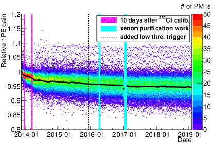
Figure 1: Time evolution of ID SPE gains relative to that in the first week of data taking for each PMT. The black points represent relative gain averaged over all ID PMTs each week. The colored points in the underlying scatter plot show the individual PMTs; the color scale represents the number of PMTs in the 0.0025 gain binning each averaged over that same week. The black dashed vertical line indicates the start of low-threshold data acquisition. The cyan and magenta bands indicate periods when data acquisition was interrupted by the Xe purification work and neutron activation after neutron source calibration.

The 1PPS data also served to monitor the ID PMTs’ dark rates by counting the number of hits in a 1 $\mu$s window before the LED flash. Figure 2 shows the time evolution of a weekly dark rate averaged over all ID PMTs, together with the “98% coverage” rate where 98% of the PMTs have a smaller dark rate than this value, and the highest rate of any single PMT. The average dark rate in all ID PMTs was 15 Hz in the beginning and had decreased to about 5 Hz by the end of data taking. This decrease in the dark rate eventually allowed us to lower the data taking and analysis thresholds.

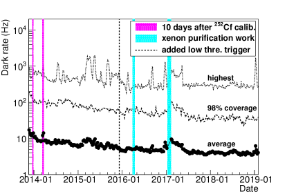
Figure 2: Time evolution of the weekly dark rate averaged over all PMTs (points), the “98% coverage” rate where 98% of the PMTs have a smaller dark rate than this value (dashed), and the highest rate of any single PMT (dotted).

When a PMT malfunction occurred, its PMT was turned off and the data from it was removed from the analysis process. This was because high rate noise often had an uncontrollable negative impact on data quality. The number of nonoperational PMTs in the ID, hereafter referred to as dead PMTs, is shown in Fig. 3 and rose from 7 to 18 over the total data-taking period. Before the large increase around April 2017, the detector had temperature cycle related to the 2nd xenon purification work, including warming up to room temperature.

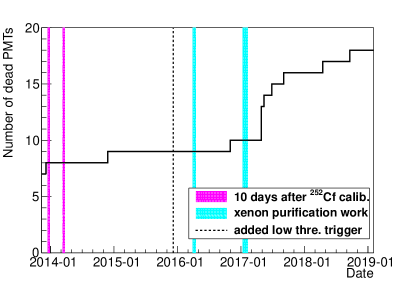
Figure 3: Number of dead ID PMTs over time.

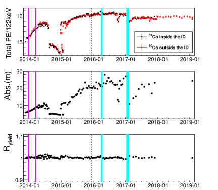
Figure 4: The top panel shows the observed total PE per 122 keV gamma rays, the black markers show ⁵⁷Co measurements made with the source inside the ID, and the red ones refer to data taken with a ⁶⁰Co irradiating the LXe target from a fixed position in the OD. The absorption length for LXe scintillation light is shown in the middle panel. The bottom panel shows the scintillation light yield ($R_{yield}$) relative to the value at the start, without taking into account the light propagation or PMT effects. The absorption length and the light yield were derived from regular ⁵⁷Co calibrations.

III.2 LXe scintillation light: yield and propagation

The PE yield in the XMASS-I detector was tracked by inserting a ⁵⁷Co source into the ID every one or two weeks. From these ⁵⁷Co calibration data [30], taken at nine different positions along the vertical z-axis through the center of the detector from $z$ = $-$40 cm to $z$ = +40 cm, the absorption and scattering lengths for scintillation light as well as the light yield of the LXe scintillator were inferred by matching the PE hit patterns in data with those of Monte Carlo (MC) simulation. The probability of the simultaneous emission of two PEs for a single LXe scintillation photon striking the photocathode of our ID PMTs [31, 32] was also properly taken into account in all our simulations.

Another way of tracking these LXe scintillation light properties was by temporarily placing a ⁶⁰Co source at the same position of the OD outside of the ID’s cryostat. A good linear correlation between the PE yield of ⁵⁷Co and that of ⁶⁰Co was then confirmed by comparing both sets of data taken on the same day during normal operation periods. This comparison allowed us to express the ⁶⁰Co data in PE per 122 keV gamma ray, the natural unit for the standard ⁵⁷Co calibration. Once the detector was stable towards the end of 2017, we suspended the more disruptive ⁵⁷Co calibration for which the source had to be inserted into the ID.

In Fig. 4 the top panel shows the resulting yield measurements and their time evolution throughout XMASS-I data taking; the black markers show ⁵⁷Co measurements made with a source at $z$ = $-$30 cm inside the ID, and the red ones refer to the ⁶⁰Co measurements, with their source deployed in the OD. The variations in the absorption length and the relative scintillation light yield $R_{yield}$ of the LXe scintillator extracted from ⁵⁷Co calibration are shown in the middle and the bottom panels, respectively. As can be seen from the figure, $R_{yield}$ was close to constant, varying within 1–2% at most. The scattering length also remained stable at around 52 cm. In our MC, an OFHC copper reflectance of 0.25+-0.05 as specular reflection was used for LXe scintillation light for the entire period. We evaluated this reflectivity using the events in the  92 keV gamma-ray peak from the progeny of ²³⁸U (²³⁴Th) in the PMT aluminum seal by comparing the data and MC. The observed changes in PE yield can be explained by corresponding variations in the absorption length. The abrupt changes around August 2014 and December 2014 were due to power outages and subsequent work undertaken to remove impurities released into the LXe during the outages. As the top panel in Fig. 4 shows, the accompanying excursions in the ID’s PE yield were largely driven by such absorption length changes [17]. From March 2015, the Xe gas evaporating from the liquid in the ID was routinely passed through a hot getter (API-Getter II, API) before being liquefied again and returning to the ID. The xenon purification work at the beginning of 2017 was a distillation to further reduce the Ar level in LXe. The decrease in PE yield and absorption length after this distillation is thought to be due to impurities (water) trapping on the refrigerator unit’s cold finger, which were released when the operation status of the one unit was changed and the unit warmed up.

III.3 Energy scale

Since the scintillation efficiency in LXe depended on the density of the energy deposit along a particle track, the estimation of energy deposited in the detector from the observed scintillation light depended on the particle that deposited the energy. Two energy deposits are of particular interest in analyzing LXe detector data: that from ER of a single electron and that from NR of a whole Xe nucleus. We denoted the amount of energy an electron would have to deposit to produce an observed amount of scintillation light as keV_ee, and the energy a recoiling Xe nucleus would have to deposit as keV_nr. The corresponding ER and NR energy scales used in this paper’s analyses are the same as the ones used in our previously published sub-GeV DM analysis [18].

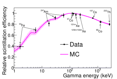
Figure 5: Relative scintillation efficiency as a function of gamma-ray energy. The efficiency at 122 keV was set to 1. The black data points were measured using gamma-ray sources in the detector, the magenta curve is what we implemented in our MC, and the band represents its one sigma error band. 1.65 keV by ⁵⁵Fe and 30.0 keV by ²⁴¹Am are the escape X-ray peaks (escaped into the source container).

Figure 5 shows the relative scintillation efficiency of gamma lines observed in XMASS-I; it is normalized to one at a ⁵⁷Co calibration line of 122 keV. Data points and their error bars come from various gamma lines observed in the spectra of the calibration sources used in our detector. The line represents how these measurements were interpolated in our MC, with the underlying band representing the variance used in the studies of our systematic uncertainties. Among the sources, ⁵⁵Fe, ²⁴¹Am, ⁵⁷Co were introduced into the ID along the z-axis, whereas ⁶⁰Co and ²³²Th sources were applied to a specified position in the OD, just outside the cryostat. We also used the xenon isotopes ^131mXe,^129mXe, and ^133mXe produced during neutron calibrations in our gamma-ray calibration. The efficiency below 5.9 keV was calibrated by the L-shell X-ray escape peaks, measured during calibration with an ⁵⁵Fe source. These escape peaks distributed energy in the 1.2–2 keV interval, with the weighted mean energies of these escape peaks being 1.65 keV and having an RMS of 0.43 keV [18].

The electron-equivalent energy scale used in this paper was constructed using the results of electron simulations based on the relative scintillation efficiency, as discussed above.

IV The data set

IV.1 Data-taking overview

The data used in this analysis were collected between November 20, 2013 and February 1, 2019. Normal data taking was organized in 24 hour ”runs” for bookkeeping and data management unless there was a specific reason to terminate a run earlier. Figure 6 shows the XMASS-I livetime accumulation over time. Data taking was interrupted twice for a few weeks (cyan colored bands in the figure): the first time, all LXe were removed from the detector so that they could be passed through a getter (SA-MT15, SAES) upon re-insertion, which removed impurities inadvertently released from a warming cold head. The second interruption allowed a distillation campaign to remove argon (Details are given in Sec. V.1). We twice used a ²⁵²Cf neutron source and had to wait for the neutron activation in the detector to abate, shown in the figure as magenta colored bands. ²⁵²Cf calibration data was used for the study of the NR scintillation decay time in LXe [33]. Regular ID calibrations were another source of dead time.

After accounting for dead time and analysis specific run selection (see below) the total collected XMASS-I livetime was 1590.9 days. Additional low threshold data taking started on December 8, 2015 with its own run selection criteria, resulting in 768.8 days of XMASS-I livetime with low threshold data.

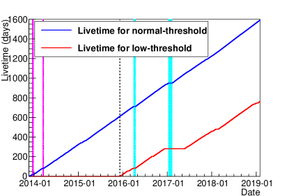
Figure 6: Livetime accumulation for normal- (blue) and low-threshold (red) data. The black dashed vertical line indicates the start of low-threshold data taking. The magenta bands represent 10-day periods after detector calibration with the ²⁵²Cf source. The cyan bands show periods of xenon purification work.

IV.2 Run selection

Runs were considered for the physics analyses presented here if they lasted at least one hour and had no DAQ problems. Figure 7 shows the stability of the LXe temperature in the ID and the pressure above the ID’s liquid surface throughout all of XMASS-I data taking. The nominal temperature and pressure of the detector were 173.0 K and 0.163 MPa, respectively. Data runs were analyzed only if their temperature and pressure were within $\pm$0.05 K and $\pm$0.5 kPa of those of their respective ID calibration runs. This ensured that changes in scintillation light yield were $<$ 0.1 %, which was verified in a study where LXe temperature and pressure were changed and their impact on PE yield checked. In this study during detector commissioning before the physics run, ⁵⁷Co source calibration was performed under different liquid xenon pressures in the XMASS detector. A 6.6$\pm$0.4 % change in light intensity was observed for a pressure change from 0.129 to 0.231 MPa with a temperature change of about 12 K. The largest temperature drop of about 0.2 K happened on Jun. 23, 2014, when the sensor providing the reference temperature for the ID temperature control loop was changed from one installed directly on the copper cold finger attached to the refrigerator to one in the pipe returning the liquefied xenon to the detector; no impact on the PE yield is evident in the top panel of Fig. 4.

Next the ID and OD trigger rates in each run were averaged over 10 minute intervals: a run would remain in the data set if none of the 10 minute averages were more than 5 sigma from the run average. We also eliminated runs in which more than 20 triggers for ID and 5 triggers for OD are issued in any one second as DAQ problems may occur beyond these limits. To avoid effects from neutron activation in the detector, runs within 10 days after a ²⁵²Cf calibration were also excluded from the data sets.

Figure 7: Time evolution of the temperature in and gas pressure above the LXe in the ID. For the temperature, its difference from the nominal temperature (see the text) is shown. The drop at the arrow was due to a change of reference sensor for controlling the cold-head that re-liquefied evaporated Xe from the target mass.

IV.3 Standard cuts applied to all ID events

A basic ID event selection, referred to as the standard cut, precedes all XMASS-I physics analyses. In the following a threshold crossing in a PMT, which for the ID PMTs leads to a readout of its waveform digitizer if it belongs to a triggered event, will be referred to as a hit, registered on the respective PMT at the time of the threshold crossing.

First, we require that the ID event under scrutiny is not associated with an OD event, that no concurrent OD event (triggered by $\geq$ 8 hits in the OD within 200 ns window) exists.

Figure 8 shows the number of hit distributions for the OD in two 24 hours runs, one at near the beginning (Jan. 2014) and the other at the end (Jan. 2019) of the data-taking period. The peak at the threshold, around ten, is mainly due to external radiation and electronic noise. Over the whole data-taking period the OD event rate increased from 0.3 Hz to 0.7 Hz for $\geq$ 8 OD PMT hits. The possible reason for this was an increase in the electronic noise, which is due to one of the PMTs becoming noisy and one new DAQ fan module. The impact of this increase in OD event rate is negligible for the analysis in this paper. The shift of the peak position around 72, shown in Fig. 8 is due to two dead OD PMTs during the data taking. To identify muon events, we required the number of OD hits more than 20. The observed muon event rate is approximately 0.17 counts per second for $\geq$ 20 OD PMT hits, which is stable throughout XMASS-I data taking and consistent with the estimated muon rate at the XMASS-I experimental site based on the muon rate at Super-Kamiokande [34].

Afterpulses are likely to occur in ID PMTs following a high energy event in the ID, and very often trigger a new ID readout all by themselves. To avoid such events consisting mainly of afterpulses, only ID events for which the trigger time difference to the preceding ID event is longer than 10 ms are retained for analysis. Counting 1PPS events affected by this cut we found that, averaged over the whole data taking period, this cut introduced 3% of additional deadtime. Afterpulse events that do occur after even longer delays are cut by checking the spread of hit timings in the event: events with a standard deviation of hit timings greater than 100 ns are also discarded as afterpulse events. Decays of ⁴⁰K in ID PMT’s photocathodes often emit Cherenkov radiation in the PMT’s quartz window. Events with more than 60% of their PMT hits registered in the first 20 ns of the event are discarded as Cherenkov events [12].

Figure 9 shows time evolution of the XMASS-I normal threshold event rate and the effect from the above selection criteria.

Figure 8: The number of hit distributions for the OD in runs at the beginning (black) and the end (red) of the data-taking period.

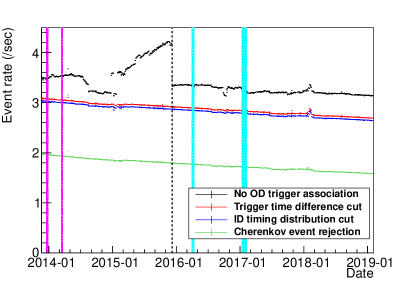
Figure 9: Time evolution of the normal threshold event rate after the reduction steps of the standard cut.

V WIMP search in XMASS-I fiducial volume analysis

Given that XMASS-I data was dominated by background originating from $\beta$ events at the ID PMTs entrance window seal at 30 keV_ee or less, a fiducial volume (FV) analysis was developed in [16] to reduce this background. Following [16], we used two different position reconstruction methods. One is based on hit timings [35], and the other is based on PE distribution [11]. These methods are referred to as $R(T)$, and $R(PE)$, respectively. We used radii $R(T)<$ 38 cm and $R(PE)<$ 20 cm for the FV selection. The fiducial target mass in this volume is 97 kg. The systematic error associated with this reconstruction is discussed in Sec. V.3.

Figure 10 shows the selected events’ PE distribution before and after these two cuts in the upper panel. The lower panel in Fig. 10 shows the reconstructed energy distribution of the surviving events, taking into account the position dependence of the PE distribution. A drop in event rate below 4 keV_ee reflects the reduced reconstruction efficiency of the PE based reconstruction at lower energies.

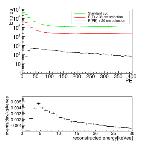
Figure 10: (Top) PE distributions for each reduction steps after standard cut. (Bottom) The reconstructed energy spectrum of data after all reductions. Reconstruction details have been explained in [11, 16, 35].

V.1 Background estimation

Here we briefly review the radio-isotopes (RI) considered in our analysis as sources of background in the FV; for details see section 4 in [16]. Below 30 keV_ee the background remaining after the above cuts was dominated by RI at the ID’s inner surface facing the LXe target mass. These events are called “mis-identified events” as their proper position reconstruction is prevented by the fact that light emitted at the inner OFHC copper surface has no direct path to the nearest PMTs’ photocathodes, leading to their PE-based reconstruction being drawn into the FV. Candidates for such RI were ²³⁸U, ²³⁵U, ²³²Th, ⁴⁰K, ²¹⁰Pb and their progeny in and on the ID’s inner surface materials. Detector elements directly facing the LXe at the ID’s inner surface were the PMTs’ entrance windows, the OFHC copper rings around each ID PMTs’ entrance window/metal body connection, and the OFHC copper plates covering these copper rings in the direction of the detector center and in particular also the gaps between the rings of neighboring PMTs. Below these was the massive OFHC copper structure that supported the PMTs, held them in their position, and further shielded the ID’s LXe target volume from external gammas.

All detector materials - except the LXe target material itself - were assayed in high purify germanium (HPGe) detectors [36] and crucial inner surface materials also in a high efficiency surface alpha counter [37]. Our background model was verified against the first 15 days of data taken and subsequently applied to all data, accounting for the decays of in particular ⁶⁰Co ($t_{1/2}=5.27$ yr) and ²¹⁰Pb ($t_{1/2}=22.2$ yr) [16].

Some RI were found to be dissolved in the LXe itself; their distribution within the target material was assumed to be uniform. For this kind of background ²²²Rn and its daughter nuclei, ⁸⁵Kr, ³⁹Ar and ¹⁴C were considered in our analysis. ²²²Rn and ⁸⁵Kr concentrations were measured using coincidences in their respective decay chains as observed in the XMASS-I detector itself. An argon contamination found in measurements of xenon gas samples from the detector volume using gas chromatography–mass spectrometry (GC–MS) was subsequently reduced in the distillation campaign. We also assumed that carbon-containing impurities contaminated the xenon, and the amount of ³⁹Ar and ¹⁴C were determined by fits to the energy spectrum above 30 keV_ee.

Our MC simulation of these background sources (BG-MC) used the quantitative evaluations outlined above and traced changes related to changes in the Xe circulation pattern over the lifetime of the full data set. The simulation also took into account changes of optical parameters (the PE yield and the absorption length shown in Fig. 4, and the scattering length) as traced in our calibrations. As already mentioned their expected change of rate due to decay was properly taken into account for the isotopes ⁶⁰Co and ²¹⁰Pb. The BG-MC output was then processed using the same selection criteria as was used for the data. Figure 11 shows the spectral composition of our BG-MC for its selected FV events in the upper panel. The systematic error of the quadratic sum of all components of this BG-MC evaluation is also shown as the red band in the figure’s lower panel, and will be further discussed in Sec. V.3.

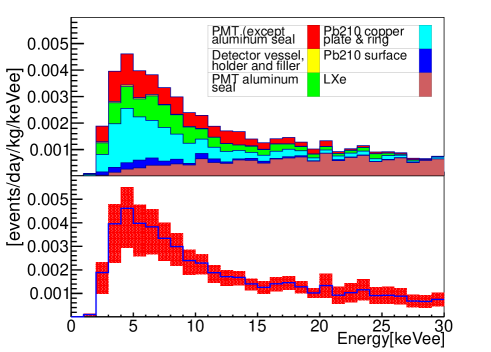
Figure 11: Energy distributions of the BG simulation after event selection from 0 to 30 keV_ee (Top) Colored stacked histograms showing the contributions from various detector components. (Bottom) A cumulative energy spectrum showing the XMASS-I BG-MC with its systematic error band.

V.2 Dead PMT induced FV events

We also describe how we correct for events pulled into the FV due to missing information from dead PMTs. This correction was carefully updated for this analysis over what was used in [16] to address the increase of number of dead PMTs in the later part of the dataset as shown in Fig. 3. The dead PMT correction originates from the observation that our event reconstruction accumulated excess events after selection in front of dead PMTs, a phenomenon that can be mimicked and verified in data by masking active PMTs in a reconstruction. These excess events presumably originate from $\beta$ events near a dead PMT’s entrance window seal, but given that the PMT is not read out by the DAQ any more, no signal is recorded on that particular PMT itself. In the PE reconstruction, which the FV cut was based on, this missing information pulls them into the FV where they appear in front of the dead PMT. Since dead PMTs are also taken into account in the XMASS MC, ideally the effect should be reproduced. However, there is a difference in the strength of the attracting effect between the results of reconstructions on events with masked PMT information in real data and similar treatment in XMASS MC data. We speculate that this difference is due to inadequate optical modelling of the PMT.

A correction factor for the BG-MC spectrum is applied for such differences in each of the energy regions 2-5, 5-15, 15-20 and 20-30 keV. These correction factors were estimated by comparing of the distance between the projection of the reconstructed vertex onto the detector surface and the dead PMT position ($D_{dead}$) between data and BG-MC in the fiducial volume. In smaller $D_{dead}$ region the effect due to dead PMT increases and in larger $D_{dead}$ region the effect decreases. In the correction calculation, to estimate effects from other than dead PMT, the $D_{dead}$ region where the effect of dead PMT becomes negligible was estimated. The number of events of the data and MC in this region was used to normalize the $D_{dead}$ distributions and then differences in distributions were evaluated. This region for normalization was estimated as $D_{dead}>$20 cm. Since the $D_{dead}$ distribution naturally depends on the number of dead PMTs, it was required to update this boundary value from the previous analysis.

Three different systematic errors were associated with this dead PMT correction. The first stemmed from the statistical uncertainty of the correction factor itself. The second contribution was estimated by the difference in the correction factor estimated from the systematic difference of event rates in the fiducial volume by deliberately masking normal PMTs. The third systematically considered the possibility that the dead PMT effect reached farther than the 20 cm boundary used in our estimation.

Figure 12 shows the actual correction factor with its the associated systematic error at the upper panel. The lower panel shows the total BG-MC after this correction is applying and its associated total systematic uncertainty reflected by the underlying green band.

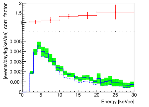
Figure 12: (Top) The dead PMT correction factor with its associated systematic error. (Bottom) The total BG-MC energy spectrum before (dotted) and after (solid) applying the dead PMT correction. The green band shows the range of this correction’s systematic uncertainty.

V.3 Systematic errors in BG-MC

The lower panel of Fig. 11 shows the BG-MC spectrum with its total systematic error as the quadratic sum of all its components. Table 1 summarizes this analysis’ systematic error estimates for the energy ranges relevant to this analysis. Its rows are organized thematically: (1) to (5) were due to the structure and properties of the ID’s inner surface. Therefore, the respective geometries were varied in the MC to explore the relevant range and obtain these values. (6) quantified effects of our PE-based position reconstruction, in particular that of the FV cut, and (7) the uncertainty in the scintillation light’s emission time constant. (8) stemmed from the dead PMT correction as explained above in Sec. V.2. (9) summarized the uncertainty in the LXe optical properties as reviewed in Sec. III. These systematic errors are not symmetric, because the number of events in the FV does not increase or decrease symmetrically with a change in these parameters as reconstructed event positions depend on them.

Table 1: BG-MC simulation systematic error by each content. Ring means a copper ring around each PMTs’ window/metal. See Fig. 1(b) in  [16] for detail. As the surface roughness of this ring affects the optical reflection property, a systematic error was introduced to account for its uncertainty. The timing response includes both the scintillation decay time and the fluctuation in the PMT.

Contents	Evaluated systematic errors
	2-5 ${\rm keV_{ee}}$	5-10 ${\rm keV_{ee}}$	10-15 ${\rm keV_{ee}}$	15-30 ${\rm keV_{ee}}$
(1) Gaps between adjacent plates	+9.1/-33.4$\%$	+5.2/-19.1$\%$	+3.1/-11.3$\%$	+1.6/-6.0$\%$
(2) Ring roughness	+9.7/-10.3$\%$	+5.6/-5.9$\%$	+3.3/-3.5$\%$	+1.8/-1.9$\%$
(3) Cu reflectivity	+3.6/-0.0$\%$	+5.9/-0.0$\%$	+4.4/-0.0$\%$	+2.4/-0.0$\%$
(4) Unevenness due to thin plate buckling	+0.0/-6.7$\%$	+0.0/-3.8$\%$	+0.0/-2.3$\%$	+0.0/-1.2$\%$
(5) PMT aluminum seal	+1.0/-1.0$\%$	+0.3/-0.3$\%$	+0.0/-0.0$\%$	+0.0/-0.0$\%$
(6) Reconstruction	+8.9/-8.9$\%$	+1.4/-7.8$\%$	+2.8/-2.8$\%$	+2.8/-2.8$\%$
(7) Timing response	+3.1/-9.9$\%$	+7.6/-11.3$\%$	+0.4/-5.3$\%$	+0.4/-5.3$\%$
(8) Dead PMT	+7.5/-7.5$\%$	+11.9/-11.9$\%$	+11.4/-11.4$\%$	+28.3/-28.3$\%$
(9) LXe optical property	+0.9/-6.7$\%$	+0.9/-6.7$\%$	+0.8/-6.7$\%$	+1.5/-1.1$\%$

V.4 Results and discussion

To search for a potential WIMP signal the observed energy spectrum was fit as the sum of the corrected BG-MC and a simulated signal contribution of unknown size. For the WIMP signal, WIMP-nucleus elastic scattering events were simulated for WIMP masses from ${\rm 20\,GeV/c^{2}}$ to ${\rm 10\,TeV/c^{2}}$. For these simulations we assumed the parameters usually used to report such results: the standard spherical and isothermal galactic halo model with a solar system speed of ${\rm v_{0}=220\,km/s}$, a Milky Way’s escape velocity of ${\rm v_{esc}=544\,km/s}$ [38]. and a local DM halo density of ${\rm 0.3\,GeV/cm^{3}}$, following Ref. [39]. The same event selection that was applied to data and BG-MC was also applied to the WIMP MC.

In the fits of the data to the sum of the dead PMT corrected BG-MC plus the simulated WIMP response of the detector for a specific WIMP mass in the energy range of 2–15 keV_ee for WIMPs we used the following $\chi^{2}$ definition:

$$\chi^{2}=\sum_{i}\frac{(D_{i}-B_{i}^{*}-\alpha\cdot W_{i}^{*})^{2}}{D_{i}+\sigma^{*}(B_{stat})_{i}^{2}+\alpha^{2}\cdot\sigma(W_{stat})_{i}^{2}}+\chi_{pull}^{2}\\ .$$ (1)

$$B_{i}^{*}=\sum_{j}p_{j}(B_{ij}+\Sigma_{k}q_{k}\cdot\sigma(B_{sys})_{ijk}),\\$$ (2)

$$W_{i}^{*}=W_{i}+\sum_{l}r_{l}\cdot\sigma(W_{sys})_{il},\\$$ (3)

$$\sigma^{*}(B_{stat})_{i}^{2}=\sum_{j}p_{j}^{2}\cdot\sigma(B_{stat})_{ij}^{2},\\$$ (4)

$$\chi_{pull}^{2}=\sum_{j}\frac{(1-p_{j})^{2}}{\sigma(B_{RI})_{j}^{2}}+\sum_{k}q_{k}^{2}+\sum_{l}r_{l}^{2},$$ (5)

where $D_{i}$, $B_{ij}$, and $W_{i}$ are the number of events in the data, the BG estimate, and WIMP MC simulations, respectively. $i$ enumerated the energy bins from 2 to 15 keV_ee (13 bins). $\alpha$ is free parameter in the fit and a scaling factor for the WIMP MC contribution corresponding to the WIMP-nucleon cross section. Therefore, the number of degrees of freedom (n.d.f.) for the fit was 12. The variable $j$ enumerated the BG sources (20 components) in the BG-MC [16]. The variables $k$ and $l$ enumerated the different systematic errors in the BG estimate (9 components) and WIMP MC simulations (4 components), respectively. ${\sigma(B_{stat})_{ij}}$ and ${\sigma(W_{stat})_{i}}$ are the statistical uncertainties in the BG estimate and the WIMP MC simulations, respectively. $\sigma(B_{RI})_{j}$, $\sigma(B_{sys})_{ijk}$, and $\sigma(W_{sys})_{i}$ are uncertainties in the amount of RI activities, systematic errors in the BG estimate (Table 1) and the WIMP MC simulations, respectively. $p_{j}$, $q_{k}$, and $r_{l}$ are scale factors for the amount of RI activity, the systematic errors in the BG estimate, and the systematic errors in the WIMP MC simulations, respectively. They were varied with constraints from the pull term shown in the equation (5) in finding minimum chi-squared value. As shown in Table 1, the amount of the systematic errors in the BG estimate ($\sigma(B_{sys})_{ijk}$) is different between positive and negative in most cases. A positive value of $\sigma(B_{sys})_{ijk}$ is chosen if $q_{k}\geq 0$, on the other hand a negative value is chosen if $q_{k}<0$.

Signal efficiency is defined as the number of retained WIMP events after applying event selections divided by the number of WIMP events generated in the FV of the detector. Systematic uncertainties for signal spectrum prediction were evaluated as shown in Ref. [16]. The largest systematic error came from the uncertainty in the scintillation decay time of ${\rm 26.9^{+0.8}_{-1.2}\,ns}$ for NR, which had been updated to reflect the latest results from our ${\rm{}^{252}Cf}$ neutron calibrations [33]. Since the Cherenkov cut affects some of the expected WIMP signal, the change in this decay time also changed the signal efficiency. Efficiencies of the WIMP signal after applying the standard, $R(T)$, and $R(PE)$ cuts, averaged over the energy ranges 2–5, 5–10, and 10–15${\rm\,keV_{ee}}$ were $12\,\%$, $32\,\%$, and $48\,\%$, respectively, for ${\rm 60\,GeV/c^{2}}$ WIMPs. The spectrum fit for these ${\rm 60\,GeV/c^{2}}$ WIMPs is shown in Fig. 13. This best fit to our BG estimate plus signal model had a $\chi^{2}$ of 12.4 (n.d.f.=12) with a null WIMP contribution ($\alpha$=0). As the observed event distribution is thus consistent with our BG evaluation, a $90\%$ confidence level (CL) upper limit on the WIMP-nucleon cross section is calculated such that the integral of the probability density function $\exp(-\Delta\chi^{2}/2)$, where $\Delta\chi^{2}=\chi^{2}-\chi^{2}_{min}$, becomes $90\%$ of the total at the limiting cross-section. The red dotted line in this figure corresponds to the signal contribution at that $90\%$ CL upper limit for ${\rm 60\,GeV/c^{2}}$ WIMPs.

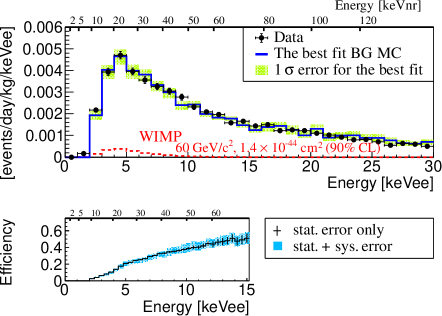
Figure 13: Data spectra with the statistical error shown in filled dots, and the BG estimate shown in a thick line with the $1\sigma$ error from the best fit shown as a shaded band with an energy region between ${\rm 2\,keV_{ee}}$ and ${\rm 30\,keV_{ee}}$ (top). The WIMP MC expectation for ${\rm 60\,GeV/c^{2}}$ is also shown in a dotted line with energy region between ${\rm 2\,keV_{ee}}$ and ${\rm 15\,keV_{ee}}$. Energy in keVnr is shown on the top. The bottom shows the signal efficiency after applying same event selections.

Such fits of the respective simulated detector response to a WIMP interaction plus the dead PMT corrected BG-MC were done for all simulated WIMP masses, and the resulting $90\%$ CL upper limits for different WIMP masses are plotted in Fig. 14. Our lowest limit is ${\rm 1.4\times 10^{-44}\,cm^{2}}$, attained at a WIMP mass of ${\rm 60\,GeV/c^{2}}$ from the fit shown in Fig. 13. This is the most stringent limit among results from single-phase LXe detectors.

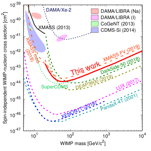
Figure 14: The spin-independent WIMP-nucleon cross section limit as a function of the WIMP mass at the $90\%$ CL for this work is shown as a solid thick line. Limits  [16, 12, 17, 41, 9, 40, 10, 7, 5, 8] as well as allowed regions  [42, 43, 44] from other experimental results are also shown.

VI Annual modulation WIMP search

The velocity of the earth relative to the galactic DM halo changes as the Earth moves around the sun. This is because the Earth’s velocity in its orbit around the Sun effectively adds to or subtracts from the Sun’s velocity through a stationary halo. This causes a corresponding change in the expected DM signal rate of terrestrial detectors, with this relative velocity modulation affecting signal rates [45]. Searches using this tell-tale signal rate modulation were already conducted with parts of the XMASS-I data for NRs from multi-GeV WIMPs [14, 17], as well as for the sub-GeV mass region where bremsstrahlung is expected to boost the signal [18]. Here we updated these results using our final five-year data set and full three years of low threshold data, as shown in Table 2. A new search exploiting the Migdal effect [46] in the sub-GeV WIMP mass region was added to this paper.

Table 2: Annual modulation data sets and their thresholds

threshold	date	PE	keVee	keVnr
low	Dec.8.2015 - Feb.1.2019	2.3	0.5	2.3
normal	Nov.20.2013 - Feb.1.2019	6.0	1.0	4.8

For these analyses, data were binned in live time intervals of roughly 15 live days per bin, resulting in 125 bins for the normal and 67 bins for the low threshold data. Both normal and low-threshold triggered events ranging in energy from 0.5 to 20 keV_ee (2.3 to 99.6 keV_nr) were used for the NR analysis. The energy range for both the bremsstrahlung and Migdal analyses was 1 to 20 keV_ee, using only normal threshold data. The 1 keV_ee energy threshold for these ER signals was set as the uncertainty in the scintillation efficiency for electrons and gamma rays increases considerably below that energy. Though the response below 1 keV_ee was implemented in the XMASS MC, the ER signal below 1 keV_ee was not considered. The scintillation efficiency and the uncertainty above 1keV_ee is shown in Fig. 5.

All modulation analyses including NR analysis were done with keV_ee unit.

VI.1 Analysis and results of multi-GeV WIMPs

The spin-independent NR signal in the energy range from 0.5 to 20 keV_ee (2.3 to 99.6 keV_nr) was used to study annual modulation induced by WIMPs in the multi-GeV mass range. Events at an energy threshold of $\sim$0.5 keV_ee average a recorded detector response of 2.3 PE.

VI.1.1 Additional event and run selections

As explained in [17], an effective background reduction near the ID wall, which was the major background in this analysis, can be achieved by constructing a likelihood function ($L$) based on the sphericity and aplanarity of PE hit patterns, as well as the fraction of the PE counts on the ID PMT with the largest PE signal to the total PE count recorded on all ID PMTs in the event. With $L_{s}$ denoting the likelihood for a signal event uniformly distributed in the target mass and $L_{b}$ the likelihood for a background event near the wall ID’s inner surface (wall event), the cut parameter in –ln($L_{s}/L_{b}$) was chosen so that it kept 50% efficiency for signal after the standard cuts. The actual cut parameter, therefore, depends on the total PE in the event.

Another significant background component in the low-threshold data stemmed from the light emission of ID PMTs [47]. Such light emission could be triggered by even only a single PE being released from the photocathode in the emitting PMT. At room temperature we measured the probability for such emission from a single PE on several PMTs and found it to be in the range of $\sim$0.3–1.0%. Given that this light emission could also occur after dark counts initiated by the thermal emission of an electron from the photocathode, the dark rate of ID PMTs directly affects the event rate at the analysis threshold. To address this background, information from the LED calibration as discussed in Sec. III, PMT dark rates and also PMT gains were used for the additional run selection. Averages and dispersion of these parameters were evaluated for two days periods and two day periods with statistically significant deviations were removed from low-threshold data set. The longest period to be removed was the one after the Xe purification work at the beginning of 2017, together with the period rejected by the run selection mentioned in Sec. IV.2. These removed period can be seen in Fig. 15 as gaps of 0.5–20keV_ee event rate.

Events with this light emission are also characterized by specific relative timing and positioning of the respective hits; the time difference between the hit caused by such light emission and the hit causing such light emission was larger than 35 ns, and the angle between the line connecting the positions of these two PMTs and the line connecting the first hit PMT and the center of the ID was smaller than 50 degrees. Only for three hit events, an additional condition was placed, requiring that no pair of the three hits met the above conditions on relative timing and angle: if any pair met these conditions, the event was not used in the analysis. The contribution from this light emission was negligible for events with larger than four hits. This additional event selection is referred to as the flasher cut.

Figure 16 shows the energy spectra for the whole data set after all selection criteria have been applied and the spectra of some simulated NR signal spectra for comparison. The time evolution of the event rate before selection and after all selections are shown in Fig. 15.

The expected annual modulation amplitude in the DM NR signature was discussed as in [39] and evaluated in the same way as in our previous XMASS analysis [14, 17, 18].

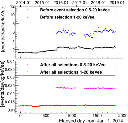
Figure 15: Time evolution of the event rate before selection (top panel) and after all selections (bottom panel). Blue and magenta show 0.5–20keV_ee event rates and 1–20keV_ee is shown by black and red.

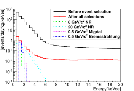
Figure 16: Energy spectra of observed data before and after event selection, and those of some simulated signal shapes: NR from 8 and 20 GeV WIMPs with $10^{-41}$, $10^{-42}\rm{cm}^{2}$ cross sections, and a Migdal and a bremsstrahlung simulation for 0.5 GeV WIMPs with cross sections of $6\times 10^{-34}\rm{cm}^{2}$ and $3\times 10^{-32}\rm{cm}^{2}$, respectively.

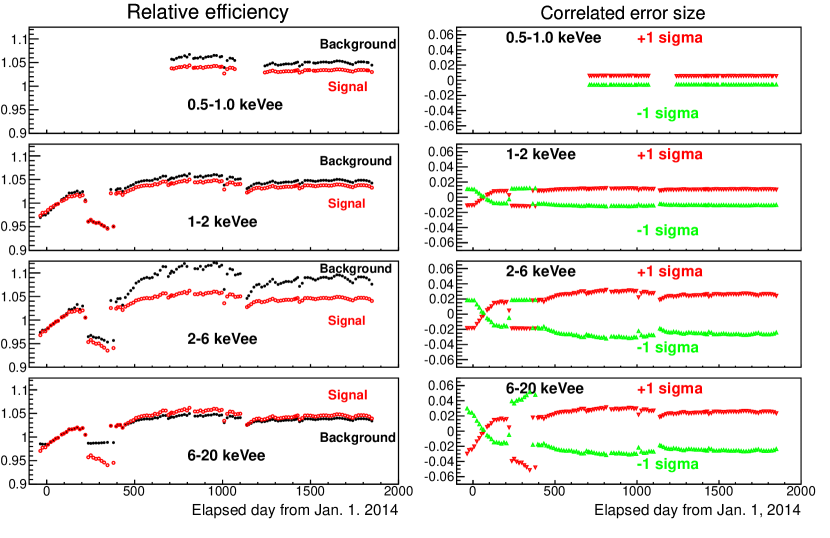
Figure 17: (Left) Relative efficiency mean values for both signal (red open circle) and background (black closed circle) events: the overall efficiency was normalized at an absorption length of 8 m for all energy ranges.
(Right) 1$\sigma$ ranges of uncertainty in the BG relative efficiencies shown in the left panel. The zero crossing near day 80 is where the improving absorption length passed 8 m.

VI.1.2 Corrections and systematic errors

Since event selection efficiency depends on the PE yield, we estimated and applied a correction to compensate for observed PE yield changes particularly during the first one and a half years of data taking. This correction and related systematic errors, called relative efficiency and derived from MC simulation, were evaluated and used as described in [14, 17]. To reflect the energy dependence of this relative efficiency for both signal and background events, the energy range from 0.5$-$20 keV_ee was divided into four energy bins: 0.5–1 keV_ee, 1–2 keV_ee, 2–6 keV_ee, and 6–20 keV_ee, and the correction were evaluated separately for each energy bin. The resulting mean relative efficiency and its correlated error is shown as a function of time from January 2014 onward in Fig. 17. We normalized this relative efficiency and its uncertainty at an absorption length of 8 m for this analysis. The mean relative efficiency in the 1–20 keV_ee energy range varied from $-$5% to +10% for the background events and from about $-$5% to +4% for the signal events over the relevant absorption length range. Difference between signal and background came from difference of generated position.The majority of background occurred near the detector wall. The correlated error of this efficiency is the largest systematic uncertainty in the analysis.

Subsequently, another correction and its related uncertainty we evaluated to account for change in the number of dead PMTs over time. The majority of background events occurred in front of the PMT window or near the detector wall. Since, for such events, a large portion of the emitted scintillation light photons were not registered if the respective PMT was dead, event evaluation by the likelihood function were severely affected. The likelihood function is based on sphericity, aplanarity and the fraction of largest PE. As shown in Fig. 3, the change of the number of dead PMTs was small during the first half of data taking, but increased from 9 PMTs to 18 in the latter half, making this a significant correction. The change of selection efficiency with the increase of dead PMTs was estimated using the data taken in the 500 days from May 2015 to September 2016, a time during which the light yield was stable and the number of dead PMTs did not change, as shown in Fig. 4 and 3. Deliberately ignoring the signals on selected good PMTs in the analysis, we simulated the dead PMT effect using events from this period and thus estimated the correction factor to the selection efficiency for each of the subsequently realized dead PMT situations. The resulting energy dependent correction factors for three subsequently increased numbers of dead PMTs are shown in Fig. 18. The errors in the figure are the statistical errors from the data used in the estimation. Though the method is same as for the FV analysis in Sec. V.2 to use masking for the effect estimation, the correction in the FV analysis corrects for the difference of the dead tube effect between the observed data and the MC data, while the correction here is correcting for the dead tube effect in the observed data.

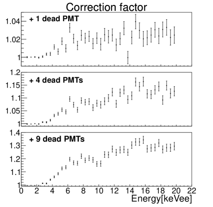
Figure 18: Dead PMT correction factors for selection efficiency at + 1, + 4, and + 9 dead PMTs periods. These corrections are applied to correct the selection efficiency from that derived for the 9 dead PMTs period. After that period, number of dead PMT started to increase significantly as shown in Fig. 3. Energy dependence of the correction factor comes from differences in the position distribution of the BG events for each energy region.

During the low-threshold data analysis the uncertainty from the flasher cut against weak light emission, explained in Sec. VI.1.1, affected the three-hit event selection by at most 0.4%.

In addition, between April 2014 and September 2014, a gain instability in the waveform digitizers contributed an extra uncertainty of 0.3% to the energy scale. During that period, a different calibration method was used for the digitizers, causing this instability. Other uncertainties stemming from the LED gain calibration, trigger-threshold stability, timing calibration, and energy resolution were negligible.

VI.1.3 Results and Discussion

For the spin-independent WIMP analysis, $\chi^{2}$ is defined as:

$$\chi^{2}=\sum\limits_{i}\limits^{E_{bins}}\sum\limits_{j}\limits^{t_{bins}}\left(\frac{(R^{{\rm data}}_{i,j}-R^{\rm ex}_{i,j}(\alpha,\beta))^{2}}{\sigma_{{\rm stat}_{i,j}}^{2}+\sigma_{{\rm sys}_{i,j}}^{2}}\right)+\alpha^{2}+\sum\limits^{N_{sys}}\limits_{i}\beta_{i}^{2},$$ (6)

where $R_{i,j}^{\rm data}$, $R_{i,j}^{\rm ex}$, $\sigma_{{\rm stat}_{i,j}}$, and $\sigma_{{\rm sys}_{i,j}}$ are the data rates and expected MC event rates, and the statistical and systematic errors of the expected event rates for the $i$th energy and $j$th time bin, respectively. The penalty term $\alpha$ relates to the overall size of the relative efficiency error, and it is common for all energy bins; therefore the size of their error simultaneously scales with $\alpha$ in the fit procedure. $\alpha$=1($-$1) corresponds to the $1\sigma(-1\sigma)$ correlated systematic error as shown in Fig. 17 (right) for the expected event rate $R^{\rm ex}_{i,j}(\alpha,\beta)$ in that energy bin. $\alpha$ is determined during $\chi^{2}$ minimization and increases $\chi^{2}$ by $\alpha^{2}$. The other penalty term, $\beta_{i}$, relates to the systematic uncertainty of the expected WIMP signal simulation. As explained in [18], this uncertainty has two main components: the scintillation efficiency and the time constant of NR signals. A time constant of 26.9${}^{+0.8}_{-1.2}$ ns was used based on our XMASS-I neutron calibration [33]. The expected signals are simulated with parameters at the limits of the 1$\sigma$ error range to estimate impacts on the amplitude $A^{s}_{i}(\beta)$ and un-modulated component $C^{s}_{i}(\beta)$ of the respective signal.

The expected modulation amplitudes become a function of the WIMP mass $A_{i}(m_{\chi})$ since the WIMP mass $m_{\chi}$ determines the recoil energy spectrum. The expected rate in bin $i,j$ is then proposed, as shown below:

$$R_{i,j}^{\rm ex}(\alpha,\beta)=\int_{t_{j}-\frac{1}{2}\Delta t_{j}}^{t_{j}+\frac{1}{2}\Delta t_{j}}\biggr{(}\epsilon^{b}_{i,j}(\alpha)\cdot(B^{b}_{i}t+C^{b}_{i})\\ +\sigma_{\chi n}\cdot\epsilon^{s}_{i,j}\cdot\big{(}C^{s}_{i}(\beta)+A^{s}_{i}(\beta)\cos 2\pi\small{\frac{(t-\phi)}{T}}\big{)}\biggr{)}dt,$$ (7)

where $\phi$ and $T$ are the modulation phase and period, then $t_{j}$ and $\Delta t_{j}$ are the respective time-bin’s center and width, $\sigma_{\chi n}$ is the WIMP-nucleon cross section, and $\epsilon^{b}_{i,j}(\alpha)$ and $\epsilon^{s}_{i,j}$ are the relative efficiencies for the background and signal, respectively, which are shown in Fig. 17 (left). To account for changing background rates from long-lived isotopes such as ⁶⁰Co (t${}_{1/2}=$5.27 yr) and ²¹⁰Pb (t${}_{1/2}=$22.3 yr), we added a linear function with $B^{b}_{i}$ for its slope and $C_{i}^{b}$ for its constant term in the $i$th energy bin. $A^{s}_{i}(\beta)$ represents an amplitude and $C^{s}_{i}(\beta)$ a constant for the un-modulated component of the signal in the $i$th energy bin after all cuts. The free parameters to be fitted are the cross section $\sigma_{\chi n}$ and $B^{b}_{i}$ and $C^{b}_{i}$ for BG, $\alpha$ and $\beta$ are constrained floating parameters. The observed $R_{i,j}^{\rm data}$ and $\sigma_{{\rm stat}_{i,j}}$ are the input parameters. To obtain the WIMP-nucleon cross section the data were fitted in the energy range from 0.5 to 20 keV_ee, assuming the same standard halo model as in Sec. V.4, with the Earth’s velocity relative to the DM halo $v_{E}=232+15~{}{\rm cos}2\pi(t-\phi)/T$ km/s. $T$ and $\phi$ were fixed to 365.24 and 152.5 days, respectively. In this analysis, the signal efficiencies for different WIMP masses were estimated from MC simulations of signal events uniformly distributed in the LXe volume.

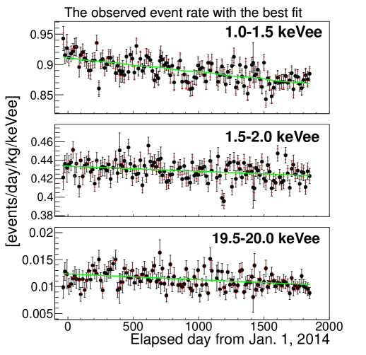
Figure 19: The observed event rate with its best fit and expected time variation for an ${\rm 8\,GeV/c^{2}}$ WIMP signal within the energy ranges of 1.0–1.5, 1.5–2.0 and 19.5–20.0 keV_ee as examples of the lowest energy bins and the highest energy bin, respectively. The black points indicate data with vertical error bars reflecting the statistical uncertainty of the count rate. The red brackets indicate the 1 $\sigma$ systematic error for each time bin. The green line indicates the best-fit result for the 8 ${\rm GeV/c^{2}}$ WIMP spectrum with the decaying BG. All data points and lines are corrected for efficiency scaled with the best-fit’s $\alpha$.

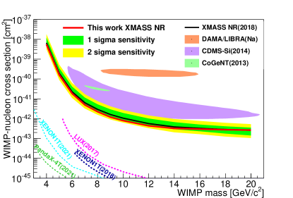
Figure 20: Limits on the spin-independent elastic WIMP-nucleon cross section as a function of WIMP mass. The solid red line shows the XMASS 90% CL exclusion from the annual modulation analysis. The solid black line shows the 2018 XMASS result [17]. The $\pm 1\rm{\sigma}$ and $\pm 2\rm{\sigma}$ bands represent the expected 90% exclusion regions. Limits, as well as allowed regions from other searches based on event counting, are also shown [7, 5, 42, 43, 44, 50].

Figure 19 shows the observed event rate with best fit and the expected time variation for ${\rm 8\,GeV/c^{2}}$ within the energy ranges of 1.0–1.5, 1.5–2.0 and 19.5–20.0 keV_ee. The best fit for the ${\rm 8\,GeV/c^{2}}$ WIMP mass had $\chi^{2}$/ndf = 4806/4734 and $\sigma_{{\chi}n}=(-1.9^{+1.6}_{-2.8})\times 10^{-42}$ cm² with the penalty term $\alpha=0.69$. Since no significant signal was observed, a 90% CL upper limit on the WIMP-nucleon cross section was set for each WIMP mass, shown in Fig. 20 by the red line. For ${\rm 8\,GeV/c^{2}}$ WIMP mass, the limit was $2.3\times 10^{-42}$ cm². Here we used the probability function $P$ defined as:

$$P={\rm exp}\left(-\frac{\chi^{2}(\sigma_{{\chi}n})-\chi^{2}_{\rm min}}{2}\right),$$ (8)

where $\chi^{2}(\sigma_{{\chi}n})$ is evaluated as a function of the WIMP-nucleon cross section $\sigma_{{\chi}n}$, and $\chi^{2}_{\rm min}$ is the minimum $\chi^{2}$ of the fit. To obtain our 90% C.L. exclusion upper limit $\sigma_{up}$, we used the Bayesian approach:

$$\frac{\int_{0}^{\sigma_{up}}Pd\sigma_{{\chi}n}}{\int^{\infty}_{0}Pd\sigma_{{\chi}n}}=0.9,$$ (9)

To evaluate our sensitivity for the WIMP-nucleon cross section, we applied our analysis to 1,000 dummy samples drawn with the same statistical and systematic errors as data, but without any modulation following the procedure described in [14]. The procedure starts by extracting an energy spectrum from the observed data. Then, a toy MC simulation was performed to vary the background event rates in each energy bin incorporating our systematic uncertainty estimates. The $\pm 1\sigma$ and $\pm 2\sigma$ bands in Fig. 20 outline the expected 90% CL upper limit band for the no-modulation hypothesis derived from these dummy samples.

VI.2 Search for sub-GeV DM

Conventional xenon detectors are sensitive to DM with sub-GeV masses based on inelastic energy transfer mechanisms involving the Migdal effect or bremsstrahlung photons occurring in NR from collisions involving even very light DM particles [48, 49].

The bremsstrahlung effect can occur when a DM collision causes a Xe nucleus to accelerate and a bremsstrahlung photon is emitted in the process. While the energy of such a photon from a DM particle of mass ${\rm 1\,GeV/c^{2}}$ is limited to 3 keV, its conversion deposits considerably more energy than is transferred in the elastic NR of such light DM particles ($\sim$0.1 keV). The Migdal effect [46] on the other hand would lead to the emission of an electron from the Xe’s atomic shell as the recoiling nucleus accelerates. Although cross sections for the bremsstrahlung and Migdal effect are smaller than that of elastic NR ($\sim$$10^{-6}$ for Migdal, $\sim$$10^{-8}$ for bremsstrahlung at ${\rm 1\,GeV/c^{2}}$), the resulting energy deposit becomes much larger due to the inelastic nature of these electromagnetic processes, making it possible to detect recoil even from sub-GeV mass DM particles.

VI.2.1 Expected signal

The expected signal from the Migdal effect was estimated following the prescriptions in [46]. The differential cross section for this process as a function of the NR energy is:

$$\begin{split}\frac{d\sigma}{dE_{R}}\simeq\sum_{E_{ec}^{F}}\frac{1}{32\pi}\frac{m_{A}}{\mu^{2}_{N}v^{2}_{DM}}\frac{|F_{A}(q^{2}_{A})|^{2}|\mathcal{M}(q_{A})|^{2}}{(m_{A}+m_{DM})^{2}}|Z_{FI}(q_{e})|^{2},\end{split}$$ (10)

where $m_{A}$ is the physical mass of the atomic system including the electron cloud energy ${m_{A}\simeq m_{N}+N_{e}m_{e}+E_{ec}}$, the DM particle mass $m_{DM}$, the DM-nucleon reduced mass $\mu_{N}$, the DM particle velocity in the laboratory frame $v_{DM}$, the nuclear form factor $F_{A}$ for momentum transfer $q_{A}$, the invariant amplitude $\mathcal{M}$, and a factor $Z_{FI}(q_{e})$ capturing the transition probability in the electron cloud with $E_{R}\simeq\frac{q^{2}_{A}}{2m_{A}}$ and $q_{e}\simeq\frac{m_{e}}{m_{A}}q_{A}$.

The Migdal event rate per unit detector mass and time is given by:

$$\frac{dR}{dE_{R}dv_{DM}}\simeq\sum_{E_{ec}^{F}}\frac{1}{2}\frac{\rho_{DM}}{m_{DM}}\frac{1}{{\mu}^{2}_{N}}\tilde{\sigma}_{N}(q_{A})\\ \times|Z_{FI}(q_{e})|^{2}\times\frac{\tilde{f}(v_{DM})}{v_{DM}},$$ (11)

where

$$\begin{split}\tilde{\sigma}_{N}(q_{A})=\frac{1}{16\pi}\frac{|F_{A}(q^{2}_{A})|^{2}|\mathcal{M}(q^{2}_{A})|^{2}}{(m_{A}+m_{DM})^{2}},\end{split}$$ (12)

with $\rho_{DM}$ denoting the local DM density and $\tilde{f}(v_{DM})$ the DM particle velocity distribution integrated over all directions.

The energy spectrum for Migdal emission from an initial orbit (n,l) then becomes

$$\begin{split}\frac{dR}{dE_{R}dE_{e}dv_{DM}}\simeq\frac{dR_{0}}{dE_{R}dv_{DM}}\times\frac{1}{2\pi}\sum_{n,l}\frac{d}{dE_{e}}p^{c}_{q_{e}}(nl\rightarrow E_{e}),\end{split}$$ (13)

with

$$\frac{dR_{0}}{dE_{R}dv_{DM}}\simeq\frac{1}{2}\frac{\rho_{DM}}{m_{DM}}\frac{1}{{\mu}^{2}_{N}}\tilde{\sigma}_{N}(q_{A})\times\frac{\tilde{f}(v_{DM})}{v_{DM}},$$ (14)

if $p^{c}_{q_{e}}$ is the ionization probability. When calculating the expected signal in the XMASS detector the energy dependent scintillation light yield is calculated separately for electron emission from the inner shell and the subsequent de-excitation emission.

The annual modulation of the bremsstrahlung signal is evaluated in the same way as in [18]. The corresponding differential event rate is:

$$\frac{dR}{d\omega}=N_{T}\frac{\rho_{DM}}{m_{DM}}\int_{v\geq v_{\rm min}}d^{3}vvf_{v}({\bf v}+{\bf v_{E}})\frac{d\sigma}{d\omega},$$ (15)

where $N_{T}$ is the number of target nuclei per unit mass in the detector, ${\bf v_{E}}$ is the velocity of the Earth relative to the galactic rest frame, and $f_{v}({\bf v})$ is the DM velocity distribution in the galactic frame. The minimum velocity was $v_{\rm min}=\sqrt{2\omega/\mu_{N}}$ [39]. We used the same parameters as in our prior multi-GeV analysis in Sec. VI.1.3.

Figure 21 shows the expected Migdal and bremsstrahlung spectra for ${\rm 0.4\,GeV/c^{2}}$ DM interactions in June and December corresponding to the maximum and minimum relative velocity $v_{E}$, respectively, as well as the average spectrum. The resulting expected annual modulation amplitude was about 30% of the average event rate at 1 keV before considering detector effects such as energy non-linearity and resolution.

Since in this energy region the signal from NR alone is negligibly small compared to that from the Migdal effect and bremsstrahlung, a NR contribution was not considered in these analyses.

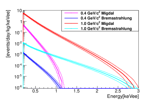
Figure 21: Expected energy spectra from Migdal effect and bremsstrahlung caused by ${\rm 0.4\,GeV/c^{2}}$ WIMPs (magenta for Migdal and cyan for bremsstrahlung) and ${\rm 1.0\,GeV/c^{2}}$ WIMPs (red for Migdal, blue for Bremasstrahlung) with a cross section of $10^{-35}\,{\rm cm}^{2}$. The dotted line shows the respective spectra in June and December, while the solid one represents the annual average spectrum. No detector effects are considered yet in these spectra.

VI.2.2 Results and discussion

For the sub-GeV DM analysis almost the same fitting procedure as discussed in Sec. VI.1.3 was applied. Differences stem from the fundamental ER nature of these signals. The expected signal rates were estimated for both Migdal effect and bremsstrahlung, with the uncertainties in the relevant scintillation decay constants and scintillation efficiency for ER signals properly considered. These uncertainties introduce correlations between energy bins in the signal spectrum. For the scintillation decay time constants, two components, referred to as the fast and the slow component, were used, based on our XMASS-I $\gamma$-ray calibrations [51]. These were 2.2 ns and 27.8${}^{+1.5}_{-1.0}$ ns, respectively, with the fast component’s fractional contribution at 0.145${}^{+0.022}_{-0.020}$.

Signal spectra were calculated for DM masses from ${\rm 0.32}$ to ${\rm 1\,GeV/c^{2}}$ for bremsstrahlung and from ${\rm 0.35}$ to ${\rm 4\,GeV/c^{2}}$ for Migdal mediated signals. The lower limits of these mass ranges were determined by the requirement to deposit more than 1 keV_ee in the detector. Below that DM mass, the expected number of events which deposit more than 1 keV_ee decrease sharply. The higher limit of ${\rm 1\,GeV/c^{2}}$ for bremsstrahlung is same as used in [18], and is based on the same assumptions as made for the signal calculation in [48]. The upper limit of ${\rm 4\,GeV/c^{2}}$ seems reasonable as beyond this energy the sensitivity of the conventional NR analysis becomes much higher than that of the bremsstrahlung and Migdal analyses.

The best fit cross section from our data was $(-2.8^{+1.5}_{-2.0})\times 10^{-35}$ cm² at ${\rm 0.5\,GeV/c^{2}}$ for the Migdal analysis with a $\chi^{2}$/ndf of 4739/4670, and the penalty term $\alpha$ becoming ${\rm 0.67}$. The result of the DM searches via Migdal and bremsstrahlung effects in the sub-GeV WIMP mass region is shown in Fig. 22. The expected sensitivity for the null-amplitude case was again calculated using toy MC samples. The 90% CL sensitivity for DM at ${\rm 0.5\,GeV/c^{2}}$ was $(2.7^{+1.3}_{-0.9})\times 10^{-35}$ cm² (the range containing 68% of the toy MC samples) for the Migdal analysis and $(2.0^{+1.0}_{-0.6})\times 10^{-33}$ cm² for the bremsstrahlung analysis. Our upper limits with a p-value of 0.09 for ${\rm 0.5\,GeV/c^{2}}$ were 1.38 $\times 10^{-35}$ cm² for Migdal and 1.1 $\times 10^{-33}$ for bremsstrahlung.

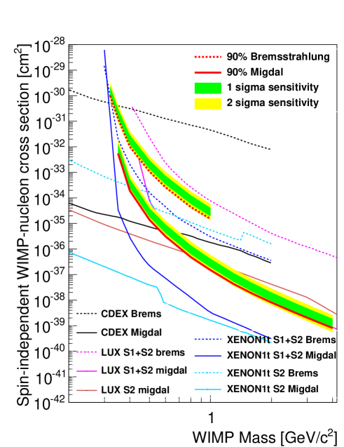
Figure 22: Summary of the sub-GeV DM analysis results considering annual modulation with the Migdal effenct and the bremsstrahlung. The red solid line is the result of the Migdal analysis for 0.35-4$\,{\rm GeV/c^{2}}$ WIMP mass, the red dotted line is the result of the bremsstrahlung analysis for 0.32-1$\,{\rm GeV/c^{2}}$. Limits from other experiments obtained via Migdal and Bremsstrahlung effect are also shown for comparison [6, 52, 53, 54].

VI.3 Model-independent analysis

For the model-independent analysis, our $\chi^{2}$ was defined, as shown below.

$$\chi^{2}=\sum\limits_{i}\limits^{E_{bins}}\sum\limits_{j}\limits^{t_{bins}}\left(\frac{(R^{{\rm data}}_{i,j}-R^{\rm ex}_{i,j})^{2}}{\sigma({\rm stat})^{2}_{i,j}+\sigma({\rm sys})^{2}_{i,j}}\right)+\alpha^{2},$$ (16)

with the expected event rate being

$$R_{i,j}^{\rm ex}=\int_{t_{j}-\frac{1}{2}\Delta t_{j}}^{t_{j}+\frac{1}{2}\Delta t_{j}}\left(\epsilon^{s}_{i,j}A^{s}_{i}\cos 2\pi\small{\frac{(t-\phi)}{T}}\right.\\ \left.+\epsilon^{b}_{i,j}(\alpha)(B^{b}_{i}t+C^{b}_{i})\right)dt,$$ (17)

where $C_{i}^{b}$ and $A_{i}^{s}$ are free parameters for the unmodulated event rate and the modulation amplitude without absolute efficiency correction, respectively. In the fitting procedure, the energy range 1–20 keV_ee was used, the modulation period $T$ was fixed to one year (= 365.24 days), and the phase $\phi$ was fixed to 152.5 days ($\sim$2nd of June), the time when the Earth’s velocity relative to the DM distribution is expected to be maximal.

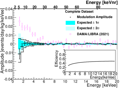
Figure 23: Modulation amplitude as a function of energy for the model-independent analysis using the pull method (black cross). Solid lines represent the 90% positive (negative) upper limits on the amplitude. The $\pm 1\rm{\sigma}$ and $\pm 2\rm{\sigma}$ bands represent the expected amplitude fluctuation ranges for a null result (for details, see text). The small figure at bottom right shows the signal efficiency used in the model-independent analysis, the overall efficiency for a uniformly distributed electron signal after applying all selection criteria. The latest DAMA/LIBRA result (square) is shown for reference [55].

The best-fit in the energy region between 1 and 20 keV_ee for our modulation hypothesis, with the fixed phase and period as detailed above, yielded $\chi^{2}_{1}$/ndf = 4693/4635 with $\alpha=0.74\pm 0.04$. The result for the null hypothesis (fixing $A^{s}_{i}=0$) was $\chi^{2}_{0}$/ndf = 4741/4673 with $\alpha=0.74\pm 0.08$. Figure 23 shows the best-fit amplitudes as a function of energy after correcting for efficiency using the curve showed at bottom right in the same figure. The $\pm 1\rm{\sigma}$ and $\pm 2\rm{\sigma}$ bands in Fig. 23 represent our expected amplitude coverage derived again from the same dummy sample procedure as in the analyses above. A hypothesis test was also done with these dummy samples, using their $\chi^{2}$ difference $\chi^{2}_{0}-\chi^{2}_{1}$ to obtain a $p$-value of 0.14 (1.5$\sigma$) for this best-fit result.

Not to limit the models that can be checked against our data we evaluated the constraints on the positive and negative amplitudes separately in Fig. 23. The upper limits on the amplitudes in each energy bin were calculated considering separately the regions of positive or negative amplitudes by integrating Gaussian distributions based on the mean and sigma of the data (=$G(a)$) from zero. The positive or negative upper limits were derived with 0.9 for $\int_{0}^{a_{up}}G(a)da/\int_{0}^{\infty}G(a)da$ or $\int_{a_{up}}^{0}G(a)da/\int_{-\infty}^{0}G(a)da$, where $a$ and $a_{up}$ are the amplitude and its 90% CL upper limit, respectively. This method obtained a positive (negative) upper limit of $0.62~{}(-2.1)\times 10^{-2}$ events/day/kg/keV_ee between 1.0 and 1.5 keV_ee with the limits becoming stricter at higher energy. The energy resolution ($\sigma/$E) at 1.0(5.0) keV_ee was estimated to be 36% (19%), comparing our gamma ray calibration data to our MC simulation. A modulation amplitude of $\sim 2\times 10^{-2}$ events/day/kg/keV_ee was obtained by DAMA/LIBRA between 1.0 and 3.5 keV_ee [55], while our positive upper limit was $\sim 5\times 10^{-3}$ events/day/kg/keV_ee in that same energy range.

VII Conclusions

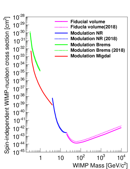
Figure 24: Limits obtained from the various analyses presented in this paper. Solid lines are the new results, using the full XMASS-I data sets, presented in this paper, in particular the fiducial volume analysis, the muliti-GeV modulation analysis via NR and the sub-GeV modulation analysis via Migdal effect and bremsstrahlung. Dotted lines show our earlier results published in [16, 17, 18]

.

XMASS-I was a unique single-phase LXe detector, which took data almost continuously over 5 full years. Over this long period of stable observation it accumulated 1590.9 live days of data with an analysis threshold of 1 ${\rm keV_{ee}}$. A subset of 768.8 days therein allows for an even lower analysis threshold of 0.5 ${\rm keV_{ee}}$.

Extending the FV search with a target mass of 97 kg to the full 1590.9 days allowed us to improve our earlier world-best single phase LXe limit on spin-independent high mass WIMP interactions by a factor of 1.6 down to ${\rm 1.4\times 10^{-44}\,cm^{2}}$ for a ${\rm 60\,GeV/c^{2}}$ WIMP at the 90$\%$ CL.

Updated searches for an annual modulation signature expected for true galactic DM halo particle interactions in terrestrial detectors, now also extended to the full XMASS-I data set and using XMASS-I’s full active target mass of 832 kg, improved on our own old limits for NR by a factor of 1.3 to reach ${\rm 2.3\times 10^{-42}\,cm^{2}}$ for a ${\rm 8\,GeV/c^{2}}$ WIMP. Also updated was our bremsstrahlung result, which for a ${\rm 0.5\,GeV/c^{2}}$ WIMP now reached a cross section limit of ${\rm 1.1\times 10^{-33}\,cm^{2}}$, an improvement of a factor 1.5. The newly added analysis exploiting the Migdal effect for low mass WIMP searches closed the WIMP mass gap that previously existed in our analyses between the lower WIMP mass end of the NR modulation analysis and the upper WIMP mass end of our bremsstrahlung based modulation analysis, reaching down to ${\rm 1.4\times 10^{-35}\,cm^{2}}$ for ${\rm 0.5\,GeV/c^{2}}$ WIMPs.

Altogether, as summarized in Fig. 24, XMASS-I WIMP searches cover the whole mass range from 0.32 to $10^{4}$ GeV/$c^{2}$ with our cross section limits in a single detector, and are the world best results from a single phase LXe detector.

References

References

- [1] S. M. Faber and J. S. Gallagher, Annu. Rev. Astron. Astrophys. 17 (1979) 135.
- [2] C. Patrignani et al., Particle Data Group, Chin. Phys. C 40 (2016) 010001.
- [3] M. W. Goodman, E. Witten, Phys. Rev. D 31 (1985) 3059.
- [4] Paolo Gondolo arXiv:hep-ph/9605290.
- [5] E. Aprile et al. (XENON Collaboration), Phys. Rev. Lett. 121 (2018) 111302.
- [6] E. Aprile et al. (XENON Collaboration), Phys. Rev. Lett. 123 (2019) 241803.
- [7] D. S. Akerib et al. (LUX Collaboration), Phys. Rev. Lett. 118 (2017) 021303.
- [8] Yue Meng et al. (PandaX-4T Collaboration), Phys. Rev. Lett. 127 (2021) 261802.
- [9] P. Agnes et al. (DarkSide Collaboration), Phys. Rev. D 98, 102006 (2018).
- [10] R. Ajaj et al. (DEAP Collaboration), Phys. Rev. D 100, 022004 (2019).
- [11] K. Abe et al., (XMASS Collaboration), Nucl. Instr. and Meth. A716 (2013) 78.
- [12] K. Abe et al. (XMASS Collaboration), Phys. Lett. B 719 (2013) 78.
- [13] U. Uchida et al. (XMASS Collaboration), Prog. Theor. Exp. Phys. (2014) 063C01.
- [14] K. Abe et al. (XMASS Collaboration), Phys. Lett. B 759 (2016) 272.
- [15] K. Abe et al. (XMASS Collaboration), Phys Rev Lett, 113, (2014) 121301.
- [16] K. Abe et al. (XMASS Collaboration), Phys. Lett. B 789 (2019) 45-53.
- [17] K. Abe et al. (XMASS Collaboration), Phys. Rev. D 97, 102006 (2018).
- [18] M. Kobayashi et al. (XMASS Collaboration), Phys.Lett. B 795 (2019) 308.
- [19] K. Abe et al. (XMASS Collaboration), Astropart. Phys. 110 (2019) 1–7.
- [20] K. Abe et al. (XMASS Collaboration), Phys.Lett. B724 (2013) 46-50.
- [21] N. Oka et al. (XMASS Collaboration), Prog. Theor. Exp. Phys. 10 (2017), 103C01.
- [22] K. Abe et al. (XMASS Collaboration), Phys. Lett. B787 (2018) 153-158.
- [23] K. Abe et al. (XMASS Collaboration), Phys. Lett. B759 (2016) 64-68.
- [24] K. Abe et al. (MASS Collaboration), Prog. Theor. Exp. Phys. 2018 (2018) 053D03.
- [25] K. Abe et al. (XMASS Collaboration), Astropart. Phys. 89 (2017) 51-56.
- [26] K. Abe et al. (XMASS Collaboration), Phys. Lett. B 809 (2020) 135741.
- [27] K. Abe et al (XMASS Collaboration), Astropart. Phys. 129 (2021) 102568.
- [28] K. Abe et al. (XMASS Collaboration), Nucl. Instrum. and Meth. A922 (2019) 171-176.
- [29] H. Ikeda et al., Nucl. Instrum. and Meth A 320 (1992) 310. S. Fukuda et al. (Super-Kamiokande Collaboration), Nucl. Instrum. and Meth. A 501 (2003) 418.
- [30] N.Y. Kim, et al. (XMASS Collaboration), Nucl. Instr. and Meth. A784 (2015) 499.
- [31] C. H. Faham et al., JINST 10 (2015) P09010.
- [32] B. López Paredes et al., Astropart. Phys. 102 (2018) 56–66.
- [33] K. Abe et al. (XMASS Collaboration), JINST 13 (2018) P12032.
- [34] G. Guillian et al. (Super-Kamiokande Collaboration), Phys. Rev. D 75, 062003 (2007).
- [35] A. Takeda for the XMASS Collaboration, Proceedings of 34th International Cosmic Ray Conference, PoS (ICRC2015) 1222.
- [36] K. Abe et al. (XMASS Collaboration), Nucl. Instrum. Meth. A922 (2019) 171-176.
- [37] K. Abe et al. (XMASS Collaboration), Nucl. Instrum. Meth. A884 (2018) 157-161.
- [38] M. C. Smith et al., Mon. Not. R. Astron. Soc. 379 (2007) 755.
- [39] J. D. Lewin, P. F. Smith, Astropart. Phys. 6 (1996) 87.
- [40] R. Agnese et al. (SuperCDMS Collaboration), Phys. Rev. Lett. 120, 061802 (2018)
- [41] R. Bernabei et al., Phys. Lett. B 436, 379 (1998).
- [42] J. Kopp et al., JCAP 03 (2012) 001.
- [43] C. E. Aalseth et al. (CoGeNT Collaboration), Phys. Rev. D 88 (2013) 012002.
- [44] R. Agnese et al. (CDMS Collaboration), Phys. Rev. Lett. 111 (2013) 251301.
- [45] A. K. Drukier, K. Freese and D. N. Spergel, Phys. Rev. D 33 3495 (1986).
- [46] M. Ibe, J. High Energ. Phys, 2018 194 (2018).
- [47] M. Kobayashi, Doctor thesis, University of Tokyo (2018)
- [48] C. Kouvaris and J. Pradler, Phys. Rev. Lett. 118,(2017) 031803.
- [49] C. McCabe, Phys. Rev. D 96 (2017) 043010.
- [50] E. Aprile et al. (XENON Collaboration), Phys. Rev. Lett. 126, 091301 (2021).
- [51] H. Takiya et al. (XMASS Collaboration), Nucl. Instr. and Meth. A834 (2016) 192.
- [52] D. S. Akerib et al. (LUX Collaboration) Phys. Rev. Lett. 122, 131301 (2019).
- [53] D. S. Akerib et al. (LUX Collaboration), Phys. Rev. D 104, 012011 (2021).
- [54] Z. Z. Liu et al. (CDEX Collaboration), Phys. Rev. Lett. 123, 161301 (2019).
- [55] R. Bernabei et al., Nucl. Phys. At. Energy 22 (2021) 329-342.
- [56] T. Doke et al., In the proceedings of the International Workshop on Technique and Application of Xenon Detectors, Xenon01, World Scientific, p. 17-27, the University of Tokyo, Japan, 3-4 December, 2001.