[section]section pageheadfoot pagenumber [0.525ex]0.6pt  [0.525ex]0.6pt [0.525ex]0.6pt  [0.525ex]0.6pt *[0.525ex]0.6pt  [0.525ex]0.6pt

Supplementary Information

This document contains the supplementary information for the paper, ‘A Bayesian approach for modelling of material stocks and flows with incomplete data’ by Wang et al.

S1 Zinc cycle system diagram

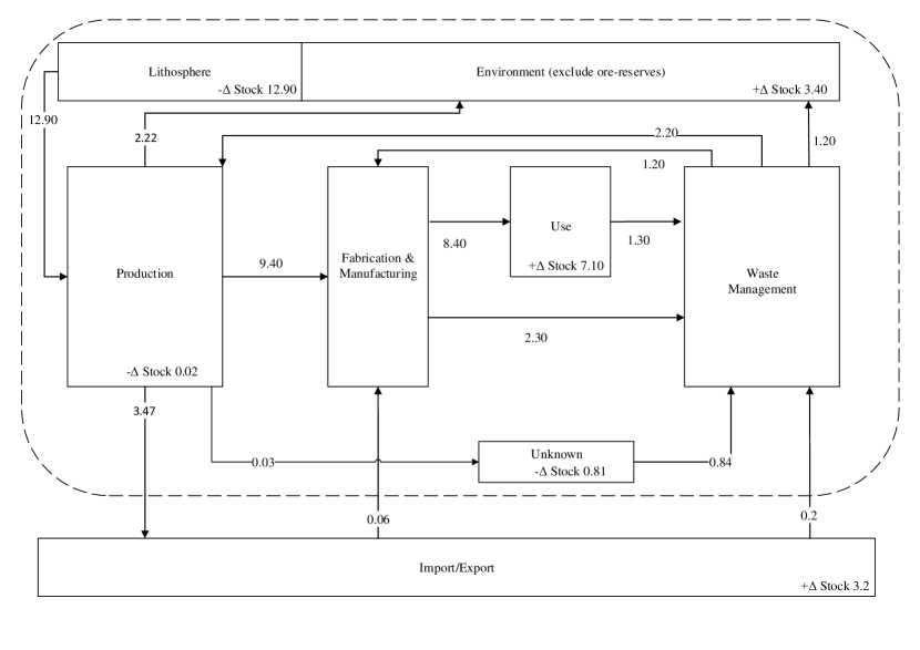
Figure S1: Zinc cycle for China, ca. 1994-1998, adapted from Figure 2d of Graedel et al. (2005). The unit of mass for zinc is displayed in $10^{5}$ metric tons per year. we explicitly define an ‘Unknown’ Process to account for flows with an unknown source or destination.

S2 Parent and child processes

In this section we elaborate on the parent and child process framework used to model disaggregation of processes or flows in MFA systems, and provide a simple illustrative example. Recall that a child process is any process which does not contain subprocesses, and a parent process is any process which does contain subprocesses. This by definition partitions all processes in the system into either child or parent processes, and all parent processes can be broken down into a set of constituent child processes. This partition of parent and child processes is useful because it allows multiple levels of disaggregation to be modelled using just two types of processes with a bottom up approach. In particular, only the child processes need to be modelled, and the parent processes variables are simply the sum of its constituent child processes variables. To illustrate this, consider the (non mass conserved) simple example of Figure S2:

Figure S2: A simple example of a MFA system with aggregation

From a typical top down approach, this example system contains 3 levels of disaggregation, since ‘Process B’ contains ‘Process A’, and ‘Process A’ in turn contains ‘Process 1’ and ‘Process 2’. In our framework however, the child processes are ‘Process 1’,‘Process 2’,‘Process 3’,‘Process 4’ and ‘Process 5’ while the parent processes are ‘Process A’, ‘Process B’ and ‘Process C’. The data in Figure S2 are the flows $U_{1,3}=1.7$, $U_{4,B}=2.3$, $U_{B,C}=10.4$ and $U_{A,5}=5.8$, and the change of stock $S_{C}=11.6$. The change in stock or flow data involving parent or aggregated processes can all be expressed in terms of flows involving child processes:

$$S_{C} =S_{4}+S_{5}$$ (S1)

$$U_{4,B} =U_{4,1}+U_{4,2}+U_{4,3}$$ (S2)

$$U_{B,C} =U_{1,4}+U_{2,4}+U_{3,4}+U_{1,5}+U_{2,5}+U_{3,5}$$ (S3)

$$U_{A,5} =U_{1,5}+U_{2,5}$$ (S4)

The data in this example can therefore be formulated with the following design matrix:

$$\setcounter{MaxMatrixCols}{12}\begin{pmatrix}0&0&1&0&0&0&0&0&0&0&0&0\\ 1&1&0&0&0&0&0&0&0&0&0&0\\ 0&0&0&0&0&0&0&0&0&1&1&1\\ 0&0&0&1&1&1&1&1&1&0&0&0\\ 0&0&0&0&1&0&1&0&0&0&0&0\end{pmatrix}\begin{pmatrix}S_{4}\\ S_{5}\\ U_{1,3}\\ U_{1,4}\\ U_{1,5}\\ U_{2,4}\\ U_{2,5}\\ U_{3,4}\\ U_{3,5}\\ U_{4,1}\\ U_{4,2}\\ U_{4,3}\end{pmatrix}=\begin{pmatrix}1.7\\ 11.6\\ 2.3\\ 10.4\\ 5.8\end{pmatrix}$$ (S5)

S3 Model diagnostics

In this section we present trace plots for a selection of change in stock and flow variables in the aluminium model, in order to check the convergence of the No-U-Turn Sampler Hamiltonian Monte Carlo algorithm. Using the No-U-Turn Sampler, we sampled 2 independent chains of $12000$ samples, with the first $2000$ samples used for tuning and discarded from the final posterior samples. The tuning samples are to give the Markov Chains iterations to converge to the target posterior distribution before extracting samples to approximate the posterior distribution. The traceplots in Figure S3 suggests both chains have converged to the same distribution. Furthermore, for both scenario A and scenario B, the Gelman-Rubin diagnostic statistic (see for example Chapter 11 of Gelman et al. (2013)) for all change in stock and flow variables in the model have converged to $1.0$ and no divergences were reported, indicating the posterior samples are reliable (Betancourt (2017)).

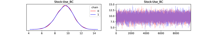
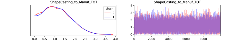
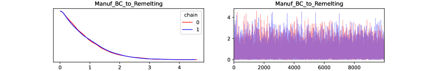
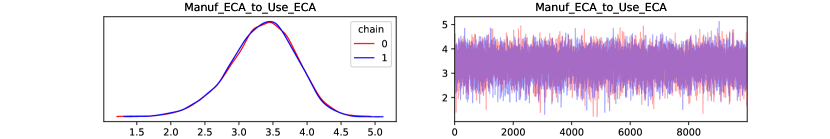
Figure S3: Traceplots for a selection of change in stock and flow variables in the aluminium model, scenario A.

S4 Detail of prior parameters for the aluminium model

In this section we give detail on the choice of prior parameters for the model evaluation of the aluminium dataset, A summary of the parameter values described in this section can be found in Table S2. Below we describe and motivate the choices:

The prior mode $\mu_{i}$ or $\mu_{j,k}$ of change in stock or flow variables respectively are chosen to be equal to the nearest power of $10$ of the reported value when it is available. For example, the flow from ‘Mining’ to ‘Refining’ with a reported value $35.4$ Mt/yr is assigned a prior mode of $\mu_{1,2}=10.0$ Mt/yr. If the flow or change in stock variable has no reported value, it is assigned an uninformative prior mode of $1.0$ Mt/yr instead.

The prior standard deviation $\sigma_{i}$ for the change in stock variables are chosen to be $\sigma_{i}=\max(\sqrt{40}\mu_{i},0.1)$, or $10.0$ if there is no reported value for the change in stock or flow variable. The corresponding parameter $\sigma_{j,k}$ for the flow variables are chosen similarly. For example, $\sigma_{1,2}=\sqrt{40}*10.0=63.25$ for the flow from ‘Mining’ to ‘Refining’. This choice is motivated by when $\mu_{i}$ is specified to the correct order of magnitude, the true value of the variable is at most $4.5\mu_{i}$ away, and so $\sigma_{i}$ is chosen on a similar scale. The maximum here is to ensure a minimum prior standard deviation of $0.1$.

The overall rationale of this choice for the prior distribution is to elicit a weakly informative prior distribution with a prior mode that captures the order of magnitude of the change in stock or flow, coupled with a relatively large prior variance, in order to reflect a realistic baseline of domain knowledge to aim for when conducting MFA.

For lack of better information, the standard deviation parameters for change in stock data noise $\tau_{i^{\prime}}$ are chosen to be $\tau_{i^{\prime}}=\max(0.1Y_{i^{\prime}},0.1)$, where $Y_{i^{\prime}}$ are the observed change in stock data. The corresponding parameters $\tau_{j^{\prime}}$ for flow data noise is chosen similarly. In other words, the data standard deviation is equal to $10\%$ of the observed data as in Lupton and Allwood (2018), but with a minimum of $0.1$ to account for a minimum degree of uncertainty from rounding or other measurement errors. For the ratio data noise, the standard deviation parameters $\tau_{k^{\prime}}$ are chosen with a somewhat smaller minimum $\tau_{k^{\prime}}=\max(0.1Y_{k^{\prime}},0.01)$, where $Y_{k^{\prime}}$ is the observed ratio.

We also ran the model assigning an Inverse Gamma prior to the standard deviation parameters of the data rather than the plug in values described in the previous paragraph. The hyperparameters of the Inverse Gamma prior for the change in stock data $a_{i^{\prime}}$ and $b_{i^{\prime}}$ are chosen as $a_{i^{\prime}}=4.0$ and $b_{i^{\prime}}=3\max(0.1Y_{i^{\prime}},0.1)$, which sets the prior mean to the plug in values $\max(0.1Y_{i^{\prime}},0.1)$ in the previous paragraph. The hyperparameters for the flow and flow ratio data are chosen similarly. However, it was found this increased computational time by about $50\%$ while only extremely marginal decreases to the posterior uncertainty of the stock and flow variables were observed. For example, in scenario A, the average posterior marginal $95\%$ HDI of all change in stock and flow variables decreased from $2.31$ to $2.28$, so we simply used the plug in values for the results presented in the main text of the paper.

For the mass conservation conditions, a small constant standard deviation of $\tau_{l^{\prime}}=0.5$ is chosen for all processes.

Parameter	Parameter prior value
$\mu_{i}$	nearest power of $10$ of reported value, or $1.0$ if unavailable
$\mu_{j,k}$	nearest power of $10$ of reported value, or $1.0$ if unavailable
$\sigma_{i}$	$\max(\sqrt{40}\mu_{i},0.1)$, or $10.0$ if reported value is unavailable
$\sigma_{j,k}$	$\max(\sqrt{40}\mu_{j,k},0.1)$, or $10.0$ if reported value is unavailable
$\tau_{i^{\prime}}$	$\max(0.1Y_{i^{\prime}},0.1)$
$\tau_{j^{\prime}}$	$\max(0.1Y_{j^{\prime}},0.1)$
$\tau_{k^{\prime}}$	$\max(0.1Y_{k^{\prime}},0.01)$
$\tau_{l^{\prime}}$	0.5
$a_{i^{\prime}}$	$4.0$
$b_{i^{\prime}}$	$3\max(0.1Y_{i^{\prime}},0.1)$
$a_{j^{\prime}}$	$4.0$
$b_{j^{\prime}}$	$3\max(0.1Y_{j^{\prime}},0.1)$
$a_{k^{\prime}}$	$4.0$
$b_{k^{\prime}}$	$3\max(0.1Y_{k^{\prime}},0.01)$

Table S1: Table of parameters for the aluminium model

S5 Detail of prior parameters for the zinc model

In this section we give detail on how the prior parameters were chosen for the zinc model. Recall that we considered two different priors for the zinc model, an uninformative prior and a weakly informative prior. For the uninformative prior, the prior modes $\mu_{i}$ of the change in stock variables are chosen to be $3.6575$ (measured in $10^{5}$ tonnes/Yr), equal to the mean of the absolute value of all the stocks and flow variables in the data, to represent a prior that only has a rough knowledge of the average order of magnitude of the system, but not the order of magnitude of each individual stock or flow. For weakly informative prior, $\mu_{i}$ are chosen the same way as the aluminium case, where the prior mode is set to the nearest power of $10$ of the ‘true’ reported value. The prior standard deviation parameters $\sigma_{i}$ are chosen to be a constant $\sqrt{40}$ in the uninformative case, and $\sigma_{i}=\max(\min(4\mu_{i},4),0.1)$ in the weakly informative case. Like in the aluminium model, $\sigma_{i}$ for the weakly informative prior is chosen at a similar scale compared to $4.5\mu_{i}$ but somewhat smaller and capped at a maximum of $4.0$ to reflect the fact that the size of flows are relatively smaller in the zinc data (when measured in $10^{5}$ tonnes/Yr, compared to the aluminium data which is measured in Mt/yr). The corresponding prior parameters for the flow variables $\mu_{j,k}$ and $\sigma_{j,k}$ are chosen similarly.

The noise standard deviation parameters of the observed data is chosen to be a constant $\tau=1.0$ throughout for all data, and similarly for the mass conservation conditions. Here the noise parameters are chosen to be somewhat larger than the aluminium model to speed up the computation of the No-U-Turn Sampler MCMC algorithm, as the model needed to be computed $2400$ times over the varying degrees of prior knowledge and available data to generate the coverage probability results in Table 1 of the main text. In particular, small values of the noise parameter induces high curvature which makes the sampling algorithm take longer to explore the posterior distribution. Similarly, for assessing point estimation (root mean squared error and maximum error) of the model on the zinc data, the posterior mode of the model is estimated directly via optimisation for faster computational speed, rather than through approximating the entire posterior distribution using MCMC.

Parameter	Parameter prior value (weakly informative prior)	Parameter prior value (uninformative prior)
$\mu_{i}$	nearest power of $10$ of reported value	$\pm 3.6575$ (sign depending if the change in stock is positive or negative)
$\mu_{j,k}$	nearest power of $10$ of reported value	$3.6575$
$\sigma_{i}$	$\max(\min(4\mu_{i},4),0.1)$	$\sqrt{40}$
$\sigma_{j,k}$	$\max(\min(4\mu_{j,k},4),0.1)$	$\sqrt{40}$
$\tau$	1.0	1.0

Table S2: Table of parameters for the zinc model

S6 Theoretical mean squared error bound on the Gaussian model

In this section we provide some theoretical analysis for the mean squared error of the Gaussian model. While the Gaussian model is a model with simplified assumptions and not the main model we advocate for MFA, it gives some intuition into why Bayesian methods perform better than non Bayesian methods in the low data setting $n\ll p$.

Owing to the closed form of the posterior of the Gaussian model described in the Methods section of the main text, we can bound the mean squared error (MSE) between the posterior mean $\bm{\mu}^{n}$ and the true parameter (stocks and flows) values $\bm{\theta}^{*}$ as follows:

Theorem 1.

Let $\tau_{i}^{2}=\tau^{2}$, in other words $T=\tau^{2}I$, $I$ the identity matrix. The mean squared error between the posterior mean of the Gaussian posterior $\bm{\mu}^{n}$ and the true stock and flow values $\bm{\theta}^{*}$ can be bounded above in the following way:

$$\mathbb{E}(\|\bm{\theta}^{*}-\bm{\mu}^{n}\|^{2}_{2})=\mathbb{E}(\sum_{j=1}^{p}(\theta_{j}^{*}-\mu_{j}^{n})^{2})$$

$$\leq\operatorname{Tr}(\Sigma^{-1/2}(\bm{\theta}^{*}-\bm{\mu})(\bm{\theta}^{*}-\bm{\mu})^{\top}\Sigma^{-1/2})\lambda_{1}(p-n+\sum_{j=1}^{n}\frac{\tau^{4}}{(d_{j}^{2}+\tau^{2})^{2}})+\tau^{2}\sum_{j=1}^{n}\frac{\lambda_{1}d_{j}^{2}}{(d_{j}^{2}+\tau^{2})^{2}}$$ (S6)

where $\lambda_{1}\geq\lambda_{2}\geq\dots\geq\lambda_{p}>0$ are the eigenvalues of $\Sigma$ in descending order, and $d_{1}\leq d_{2}\leq\dots\leq d_{n}$ are the singular values of $X\Sigma^{1/2}$ in ascending order.

The bound in Equation S6 helps to give some insight into how the mean squared error of the model evolves as more data is added. This is perhaps easiest to see in the case when $\tau$ is near $0$ (meaning the data is almost noiseless), which leaves

$$\operatorname{Tr}(\Sigma^{-1/2}(\bm{\theta}^{*}-\bm{\mu})(\bm{\theta}^{*}-\bm{\mu})^{\top}\Sigma^{-1/2})\lambda_{1}(p-n)$$

as the dominant term. The $\operatorname{Tr}(\Sigma^{-1/2}(\bm{\theta}^{*}-\bm{\mu})(\bm{\theta}^{*}-\bm{\mu})^{\top}\Sigma^{-1/2})$ part of this term can be interpreted as a measurement of how close the prior mean is to the true values of the parameters (it is $0$ when $\bm{\theta}^{*}=\bm{\mu}$) and does not depend on the data, while the factor $\lambda_{1}(p-n)$ decreases as $n$ increases, meaning as more data is added. This indicates that in a high dimensional setting $n\ll p$ which is inherent in MFA studies, the availability of informative priors is key to obtaining more accurate estimates of the true stock and flow values.

Furthermore, in the case when $\Sigma=\lambda_{1}I$, Equation S6 can be directly compared with the ridge regression case. Since ridge regression is equivalent to the case when $\bm{\mu}=\bm{0}$ and $\Sigma=\lambda_{1}I$, Equation S6 is smaller for the Gaussian model compared to ridge regression whenever $\operatorname{Tr}((\bm{\theta}^{*}-\bm{\mu})(\bm{\theta}^{*}-\bm{\mu})^{\top})=\|\bm{\theta}^{*}-\bm{\mu}\|^{2}_{2}$ is smaller than $\|\bm{\theta}^{*}\|^{2}_{2}$. In other words whenever the prior mean $\bm{\mu}$ is closer to the true value in (L2) distance than the zero vector $\bm{0}$, which is consistent with the simulations presented in the Results section of the main text.

Proof of Theorem 1.

Recall that the posterior mean of the conjugate Gaussian model can be written as:

$$\bm{\mu}^{n}=\bm{\mu}+\Sigma X^{\top}(X\Sigma X^{\top}+\tau^{2}I)^{-1}(X(\bm{\theta}^{*}-\bm{\mu})+\bm{\epsilon})$$

This can be derived from looking at the joint distribution $[\bm{\theta},X\bm{\theta}+\bm{\epsilon}]^{\top}$ and using standard Gaussian conditioning formulae:

$$\begin{bmatrix}\bm{\theta}\\ X\bm{\theta}+\bm{\epsilon}\end{bmatrix}\sim\mathcal{N}\left(\begin{bmatrix}\bm{\mu}\\ X\bm{\mu}\end{bmatrix},\begin{bmatrix}\Sigma&\Sigma X^{\top}\\ X\Sigma&X\Sigma X^{\top}+\tau^{2}I\end{bmatrix}\right)$$ (S7)

Suppose $dim(X)=(n,p)$, $dim(\Sigma)=(p,p)$, $dim(\bm{\mu})=dim(\bm{\theta}^{*})=(p,1)$, $dim(\bm{\epsilon})=(n,1)$, and we’ll assume $n<p$, since material flow analysis typically has less data than parameters. Assume $\Sigma$ is symmetric positive definite and $X$ has full rank. The mean squared error (MSE) between the posterior mean $\bm{\mu}^{n}$ and the true value $\bm{\theta}^{*}$ is equal to:

$$MSE =\mathbb{E}\|\bm{\theta}^{*}-\bm{\mu}-\Sigma X^{\top}(X\Sigma X^{\top}+\tau^{2}I)^{-1}(X(\bm{\theta}^{*}-\bm{\mu})+\bm{\epsilon})\|^{2}_{2}$$

$$=\mathbb{E}(\bm{\beta}-\Sigma X^{\top}(X\Sigma X^{\top}+\tau^{2}I)^{-1}(X\bm{\beta}+\bm{\epsilon}))^{\top}(\bm{\beta}-\Sigma X^{\top}(X\Sigma X^{\top}+\tau^{2}I)^{-1}(X\bm{\beta}+\bm{\epsilon}))$$

$$=\mathbb{E}(\bm{\beta}^{\top}(I-\Sigma X^{\top}(X\Sigma X^{\top}+\tau^{2}I)^{-1}X)^{\top}(I-\Sigma X^{\top}(X\Sigma X^{\top}+\tau^{2}I)^{-1}X)\bm{\beta})$$

$$+\mathbb{E}(\bm{\epsilon}^{\top}(\Sigma X^{\top}(X\Sigma X^{\top}+\tau^{2}I)^{-1})^{\top}\Sigma X^{\top}(X\Sigma X^{\top}+\tau^{2}I)^{-1}\bm{\epsilon})$$

Where $\bm{\beta}=\bm{\theta}^{*}-\bm{\mu}$. At this point we decompose the MSE into the bias and variance terms. Let

$$MSE_{1}=\mathbb{E}(\bm{\beta}^{\top}(I-\Sigma X^{\top}(X\Sigma X^{\top}+\tau^{2}I)^{-1}X)^{\top}(I-\Sigma X^{\top}(X\Sigma X^{\top}+\tau^{2}I)^{-1}X)\bm{\beta})$$

denote the bias term. and

$$MSE_{2}=\mathbb{E}(\bm{\epsilon}^{\top}(\Sigma X^{\top}(X\Sigma X^{\top}+\tau^{2}I)^{-1})^{\top}\Sigma X^{\top}(X\Sigma X^{\top}+\tau^{2}I)^{-1}\bm{\epsilon})$$

denote the variance term.

For the bias term, using the fact that the trace of a scalar is equal to itself and the cyclic property of trace, we have:

$$MSE_{1}=\operatorname{Tr}(\bm{\beta}^{\top}(I-\Sigma X^{\top}(X\Sigma X^{\top}+\tau^{2}I)^{-1}X)^{\top}(I-\Sigma X^{\top}(X\Sigma X^{\top}+\tau^{2}I)^{-1}X)\bm{\beta})$$

$$=\operatorname{Tr}(\bm{\beta}\bm{\beta}^{\top}(I-\Sigma X^{\top}(X\Sigma X^{\top}+\tau^{2}I)^{-1}X)^{\top}(I-\Sigma X^{\top}(X\Sigma X^{\top}+\tau^{2}I)^{-1}X))$$

$$=\operatorname{Tr}(\bm{\beta}\bm{\beta}^{\top}\Sigma^{-1/2}\Sigma^{1/2}(I-X^{\top}(X\Sigma X^{\top}+\tau^{2}I)^{-1}X\Sigma)\Sigma^{-1/2}\Sigma\Sigma^{-1/2}(I-\Sigma X^{\top}(X\Sigma X^{\top}+\tau^{2}I)^{-1}X)\Sigma^{1/2}\Sigma^{-1/2})$$

$$=\operatorname{Tr}(\Sigma^{-1/2}\bm{\beta}\bm{\beta}^{\top}\Sigma^{-1/2}(I-\Sigma^{1/2}X^{\top}(X\Sigma X^{\top}+\tau^{2}I)^{-1}X\Sigma^{1/2})\Sigma(I-\Sigma^{1/2}X^{\top}(X\Sigma X^{\top}+\tau^{2}I)^{-1}X\Sigma^{1/2}))$$

Notice $\Pi_{\tau}=\Sigma^{1/2}X^{\top}(X\Sigma X^{\top}+\tau^{2}I)^{-1}X\Sigma^{1/2}$ is symmetric. Similarly $I-\Pi_{\tau}$ is symmetric and so $(I-\Pi_{\tau})^{2}$ is positive semidefinite.

Let $X\Sigma^{1/2}=UDV^{\top}$ be the singular value decomposition of $X\Sigma^{1/2}$, where $d_{1}\leq d_{2}\leq\dots\leq d_{n}$ are the diagonal elements of $D$ (also known as the singular values of $X\Sigma^{1/2}$) arranged in ascending order, then we have:

$$\Pi_{\tau} =VD^{\top}U^{\top}(UDD^{\top}U^{\top}+\tau^{2}I)^{-1}UDV^{\top}=VD^{\top}(DD^{\top}+\tau^{2}I)^{-1}DV^{\top}$$

which has the same eigenvalues as $D^{\top}(DD^{\top}+\tau^{2}I)^{-1}D$ by similarity, which are $d_{i}^{2}/(d_{i}^{2}+\tau^{2})$ and $0$ (repeated $p-n$ times). Likewise the eigenvalues of $I-\Pi_{\tau}$ are therefore $1$ (repeated $p-n$ times) and $\tau^{2}/(d_{i}^{2}+\tau^{2})$

returning to the bias term, we have:

$$MSE_{1} =\operatorname{Tr}(\Sigma^{-1/2}\bm{\beta}\bm{\beta}^{\top}\Sigma^{-1/2}(I-\Pi_{\tau})\Sigma(I-\Pi_{\tau}))$$

$$\leq\operatorname{Tr}(\Sigma^{-1/2}\bm{\beta}\bm{\beta}^{\top}\Sigma^{-1/2})\operatorname{Tr}((I-\Pi_{\tau})^{2}\Sigma)$$

$$\leq\operatorname{Tr}(\Sigma^{-1/2}\bm{\beta}\bm{\beta}^{\top}\Sigma^{-1/2})(\sum_{j=1}^{p-n}\lambda_{j}+\sum_{j=1}^{n}\lambda_{p-n+j}\tau^{4}/(d_{j}^{2}+\tau^{2})^{2})$$

$$\leq\operatorname{Tr}(\Sigma^{-1/2}\bm{\beta}\bm{\beta}^{\top}\Sigma^{-1/2})\lambda_{1}(p-n+\sum_{j=1}^{n}\tau^{4}/(d_{j}^{2}+\tau^{2})^{2})$$ (S8)

Where we used Von Neumann’s trace inequality (Mirsky (1975)) in the penultimate line, on the matrices $(I-\Pi_{\tau})^{2}$ and $\Sigma$. So provided $\tau^{2}$ is small compared to the $d_{j}^{2}$, $MSE_{1}$ decreases approximately linearly in $n$, as $n$ increases to $p$.

For the variance term $MSE_{2}$, we once again use the singular value decomposition $X\Sigma^{1/2}=UDV^{\top}$:

$$MSE_{2} =\operatorname{Tr}(\mathbb{E}(\bm{\epsilon}^{\top}(\Sigma X^{\top}(X\Sigma X^{\top}+\tau^{2}I)^{-1})^{\top}\Sigma X^{\top}(X\Sigma X^{\top}+\tau^{2}I)^{-1}\bm{\epsilon}))$$

$$=\operatorname{Tr}(\mathbb{E}(\bm{\epsilon}\bm{\epsilon}^{\top}(\Sigma X^{\top}(X\Sigma X^{\top}+\tau^{2}I)^{-1})^{\top}\Sigma X^{\top}(X\Sigma X^{\top}+\tau^{2}I)^{-1}))$$

$$=\tau^{2}\operatorname{Tr}((X\Sigma X^{\top}+\tau^{2}I)^{-2}X\Sigma^{2}X^{\top})$$

$$=\tau^{2}\operatorname{Tr}((UDD^{\top}U^{\top}+\tau^{2}I)^{-2}UDV^{\top}\Sigma VD^{\top}U^{\top})$$

$$=\tau^{2}\operatorname{Tr}(U^{\top}(UDD^{\top}U^{\top}+\tau^{2}I)^{-1}UU^{\top}(UDD^{\top}U^{\top}+\tau^{2}I)^{-1}UDV^{\top}\Sigma VD^{\top})$$

$$=\tau^{2}\operatorname{Tr}(VD^{\top}(DD^{\top}+\tau^{2}I)^{-2}DV^{\top}\Sigma)$$

$$\leq\tau^{2}\sum_{j=1}^{n}\lambda_{1}d_{j}^{2}/(d_{j}^{2}+\tau^{2})^{2}$$

Where the last line again follows from Von Neumann’s trace inequality, on the matrices $VD^{\top}(DD^{\top}+\tau^{2}I)^{-2}DV^{\top}$ and $\Sigma$.

$\blacksquare$

References

• Betancourt [2017] M. Betancourt. A conceptual introduction to hamiltonian monte carlo. 2017. doi: 10.48550/ARXIV.1701.02434. URL https://arxiv.org/abs/1701.02434.
• Gelman et al. [2013] A. Gelman, J. Carlin, H. Stern, D. Dunson, A. Vehtari, and D. Rubin. Bayesian Data Analysis, Third Edition. Chapman and Hall/CRC, 2013. ISBN 9781439840955.
• Graedel et al. [2005] T. E. Graedel, D. van Beers, M. Bertram, K. Fuse, R. B. Gordon, A. Gritsinin, E. M. Harper, A. Kapur, R. J. Klee, R. Lifset, L. Memon, and S. Spatari. The multilevel cycle of anthropogenic zinc. Journal of Industrial Ecology, 9(3):67–90, 2005. doi: https://doi.org/10.1162/1088198054821573. URL https://onlinelibrary.wiley.com/doi/abs/10.1162/1088198054821573.
• Lupton and Allwood [2018] R. C. Lupton and J. M. Allwood. Incremental material flow analysis with bayesian inference. Journal of Industrial Ecology, 22(6):1352–1364, 2018. doi: https://doi.org/10.1111/jiec.12698. URL https://onlinelibrary.wiley.com/doi/abs/10.1111/jiec.12698.
• Mirsky [1975] L. Mirsky. A trace inequality of john von neumann. Monatshefte für Mathematik, 79(4):303–306, Dec 1975. ISSN 1436-5081. doi: 10.1007/BF01647331. URL https://doi.org/10.1007/BF01647331.