Optimal Demand Shut-offs of AC Microgrid
using AO-SBQP Method

Abstract

Microgrids are increasingly being utilized to improve the resilience and operational flexibility of power grids, and act as a backup power source during grid outages. However, it necessitates that the microgrid itself could provide power to the critical loads. This paper presents an algorithm named alternating optimization based sequential boolean quadratic programming tailored for solving optimal demand shut-offs problems arising in microgrids. Moreover, we establish local superlinear convergence of the proposed approximate Boolean quadratic programming method over nonconvex problems. In the end, the performance of the proposed method is illustrated on the modified IEEE 30-bus case study.

1 Introduction

Microgrids are small-scale power grids that can operate autonomously or in collaboration with other small power grids, which are increasingly being utilized to increase the resilience and operational flexibility of power grids. They act as a backup power supply in the case of grid outages caused by devastating disasters. Abbey et al. (2014) summarized the measures taken by Sendai region in Japan to cope with the shortage of circuit supply caused by the nuclear power accident after the 2011 East Japan Earthquake. Similarly, Panora et al. (2014) describes a successful case of rapid restoration of local microgrid integrated energy systems after infrastructure damage caused by Superstorm Sandy in Manhattan Island, 2012. However, this necessitates that each isolated microgrid itself be resistant and formulate its own optimal power supply strategy with the shortage of energy supply, which is still a challenging problem. Basically, a potential solution is to abstract the above power grid optimization problem in a mixed Boolean nonlinear programming fashion (MBNLP).

To the best of our knowledge, classical optimization in power grid consists optimal power flow (OPF, Frank et al. (2012)), optimal reactive power dispatch (Zhu (2015)), power system state and parameter estimation (Monticelli (1999); Du et al. (2019)). Recently, Du et al. (2020, 2022) proposes the method of optimal experimental design (OED) in order to extract more relative information for assisting the admittance estimation process. Moreover, Du et al. (2021) offers an adaptive method for balancing OED and the OPF cost. These mentioned power grid optimization problems are smooth and can be solved directly with interior point method, while notable recent researches optimize the discrete decision variables at the same time. Rhodes et al. (2020) and Kody et al. (2022) modeled the direct current (DC) optimal power shut-in problems in a mixed integer linear program (MILP) framework and solved them with Gurobi. However, only few literature can be found for nonconvex MBNLP in the area of alternating current (AC) power systems. On the other hand, from the algorithmic level, the solver is based on branch and bound (B$\&$B) method (Morrison et al. (2016)), which needs to establish a tree storage structure to explore each integer variable with low efficiency. Luo et al. (2010) solves Boolean optimization in a semi-definite relaxation (SDR) fashion, however, with matrix variables. Solving nonconvex MBNLP accurately and efficiently remains an open problem in our view.

Recently, a quadratic programming with linear complementary constraint (LCQP) problem is well studied by a series of literatures (Hall et al. (2021, 2022)). By sequentially solving the QP problem with the corresponding linearlized penalty term, the complementary constraint can be reached with finite steps. Inspired by the above literatures, alternating optimization based sequential boolean quadratic programming (AO-SBQP) (Zhu and Du (2022)) is proposed to set up a bridge between LCQP and MBNLP, leading the solution of optimization problems with Boolean variables no longer rely on B$\&$B method with tree structure searching or SDR with matrix variables.

In this paper, the idea of AO-SBQP method is inherited, and the algorithm is modified in the specific optimal distribution of limited supply scenario in microgrid. Unlike Zhu and Du (2022), our considered model is still a non-convex problem except the Boolean variable constraints. Moreover, a local convergence analysis for the approximate BQP with constraints is introduced.

The rest of this paper is organized as follows: Section 2 reviews the basics concepts of power grid. Sections 3 proposes the optimal distribution of limited supply model. Section 4 describes the AO-SBQP algorithm in detail. And the numerical result is shown in Section 5.

Notation: For $a\in\mathbb{R}^{n}$ and $\mathcal{C}\subseteq\{1,...,n\}$, ${[a_{i}]_{i\in\mathcal{C}}\in\mathbb{R}^{|\mathcal{C}|}}$ collects all components of $a$ whose index $i$ is in $\mathcal{C}$. Similarly, for $A\in\mathbb{R}^{n\times l}$ and $\mathcal{S}\subseteq\{1,\ldots,n\}\times\{1,\ldots,l\}$, $[A_{i,j}]_{(i,j)\in\mathcal{S}}\in\mathbb{R}^{|\mathcal{S}|}$ denotes the concatenation of $A_{i,j}$ for all $(i,j)\in\mathcal{S}$. $\mathfrak{i}=\sqrt{-1}$ denotes the imaginary unit, such that $\mathrm{Re}(z)+\mathfrak{i}\cdot\mathrm{Im}(z)=z\in\mathbb{C}$, and $\hat{a}$ denotes the estimated value of $a$. Moreover, $\mathbf{1}$ represents a vector with all entries being one.

2 AC Power Grid Model

Consider a power grid defined by the triple $(\mathcal{N},\mathcal{L},(G+\mathfrak{i}B))$, where $\mathcal{N}=\{1,2,\dots N\}$ represents the set of buses, $\mathcal{L}\subseteq\mathcal{N}\times\mathcal{N}$ denotes transmission lines and $(G+\mathfrak{i}B)\in\mathbb{C}^{N\times N}$ is the complex and potentially sparse Laplacian admittance matrix

$$(G_{k,l}+\mathfrak{i}B_{k,l})\doteq\left\{\begin{array}[]{ll}\sum\limits_{i\neq k}\left(g_{k,i}+\mathfrak{i}\,b_{k,i}\right)&\text{if}\;k=l,\\[7.11317pt] -\left(g_{k,l}+\mathfrak{i}\,b_{k,l}\right)&\text{if}\;k\neq l.\end{array}\right.$$

Here, $g_{k,l}$ and $b_{k,l}$ are the conductances and susceptances of the transmission line $(k,l)\in\mathcal{L}$, which aims to connect the buses. Note that $(G_{k,l}+\mathfrak{i}B_{k,l})=0$ if $(k,l)\notin\mathcal{L}$. The set $\mathcal{G}\subseteq\mathcal{N}$ collects all nodes equipped with generators and $\mathcal{D}\subseteq\mathcal{N}$ collects all nodes with power demands. Figure 1 shows a 5-bus system with $\mathcal{N}=\{1,\dots,5\}$, $\mathcal{G}=\{1,3,4,5\}$, $\mathcal{D}=\{2,3,4\}$.

Figure 1: Modified IEEE 5-bus system from Li and Bo (2010) with 4 generators and 3 consumers.

Let $v_{k}$ denote the voltage amplitude at the $k$-th node and $\theta_{k}$ the corresponding voltage angle, $\theta_{k,l}$ denotes the angle difference between node $k$ and $l$. Throughout this paper, we assume that the voltage magnitude and the voltage angle at the first node (the slack node) are fixed, $\theta_{1}=0\quad\text{and}\quad v_{1}=\mathrm{const}\;$. We refer to Du et al. (2021) and Du et al. (2022) for further discussion. The state variables of the system is defined as

$$x\doteq\begin{bmatrix}v_{k},\theta_{k}\end{bmatrix}_{k\in\mathcal{N}}^{\top}\in\mathbb{R}^{2|\mathcal{N}|}.\;$$

Moreover, we have active and reactive power generation of generators $p_{k}^{g}$ and $q_{k}^{g}$ for all $k\in\mathcal{G}$, and $d_{k}=(p_{k}^{d},\;q_{k}^{d})^{\top}$ denote the active and reactive power demand at demand nodes $k\in\mathcal{D}$. We consider active and reactive power supply of all generators

$$u\doteq\begin{bmatrix}p_{k}^{g},q_{k}^{g}\end{bmatrix}_{k\in\mathcal{G}}^{\top}\in\mathbb{R}^{2|\mathcal{G}|}\;$$

as the system input variables.

The active and reactive power flow over the transmission line $(k,l)\in\mathcal{L}$ is given by

$$\Pi_{k,l}(x)\doteq v_{k}^{2}\begin{bmatrix}g_{k,l}\\[4.55254pt] -b_{k,l}\end{bmatrix}$$

$$-v_{k}v_{l}\begin{bmatrix}g_{k,l},&b_{k,l}\\[4.55254pt] -b_{k,l},&g_{k,l}\end{bmatrix}\begin{bmatrix}\cos(\theta_{k,l})\\[4.55254pt] \sin(\theta_{k,l})\end{bmatrix}.$$

The total power outflow from node $k\in\mathcal{N}$ is given by

$$\begin{split}P_{k}(x)\doteq&v_{k}^{2}\sum_{l\in\mathcal{N}_{k}}\begin{bmatrix}g_{k,l}\\[4.55254pt] -b_{k,l}\end{bmatrix}\\ &-v_{k}\sum_{l\in\mathcal{N}_{k}}v_{l}\begin{bmatrix}g_{k,l},&b_{k,l}\\[4.55254pt] -b_{k,l},&g_{k,l}\end{bmatrix}\begin{bmatrix}\cos(\theta_{k,l})\\[4.55254pt] \sin(\theta_{k,l})\end{bmatrix}\\ \doteq&\sum_{l\in\mathcal{N}_{k}}\Pi_{k,l}(x),\end{split}$$

where

$$\mathcal{N}_{k}\doteq\{l\in\mathcal{N}\,\mid\,(k,l)\in\mathcal{L}\,\}$$

denotes the set of neighbors of node $k\in\mathcal{N}$.

3 Optimal Distribution of Limited Supply Power Network

In the limited power supply scenario, potentially,

$$\sum_{k\in\mathcal{G}}\overline{p_{k}^{g}}<\sum_{k\in\mathcal{D}}p_{k}^{d},$$

here, $\overline{p_{k}^{g}}$ denotes the upper bound of active generator power input of bus $k$. This leads to a fact that not all the power demand will enjoy stable energy supply. Thus we introduce $y\in\mathbb{R}^{|\mathcal{D}|}$ with $y_{k}\in\{0,1\}$ as an auxiliary switch variable. Then the power supply at a given bus can be expressed as

$$S_{k}(u,y)\doteq\left\{\begin{aligned} &\begin{bmatrix}p_{k}^{g},q_{k}^{g}\end{bmatrix}^{\top}-y^{2}_{k}\begin{bmatrix}p_{k}^{d},q_{k}^{d}\end{bmatrix}^{\top},&k&\in\mathcal{D},\mathcal{G}\\[4.55254pt] &\begin{bmatrix}p_{k}^{g},q_{k}^{g}\end{bmatrix}^{\top},\qquad&k&\notin\mathcal{D},k\in\mathcal{G}\\[4.55254pt] &-y_{k}^{2}\begin{bmatrix}p_{k}^{d},q_{k}^{d}\end{bmatrix}^{\top},\qquad&k&\in\mathcal{D},k\notin\mathcal{G}.\end{aligned}\right.$$

Thus, the power flow equations can be written in the form

$$\begin{split}&P(x)=S(u,y)\;\end{split},$$ (1)

where

$$P(x) \doteq\left[P_{1}(x)^{\top},\ldots,P_{N}(x)^{\top}\right]^{\top},$$

$$\;\;S(u,y) \doteq\left[S_{1}(u,y)^{\top},\ldots,S_{N}(u,y)^{\top}\right]^{\top}.\;$$

Notice that $\mathrm{dim}(P)=\mathrm{dim}(x)=2|\mathcal{N}|\;.$

Optimal power demand shut-offs (weighted maximum load delivery, Rhodes et al. (2020)) can be formulated in the following way for a given positive rank $r_{k}\in\mathbb{R}^{+}$ of each power demand.

$$\max_{x,u,y}\;\; f(x,u,y)=\sum_{k\in\mathcal{D}}y_{k}r_{k}p^{d}_{k}$$ (2a)

$$\quad\mathrm{s.t.}\;\; P(x)-S(u,y)=0$$ (2b)

$$\underline{x}\leq x\leq\overline{x}$$ (2c)

$$\underline{u}\leq u\leq\overline{u}$$ (2d)

$$y_{k}\in\{0,1\}.$$ (2e)

Here we are trying to provide stable power supply for the most important consumers with limited resource. Unlike other classical optimization problems over power grid (Zhu (2015), Frank et al. (2012)), the Boolean variable $y$ leads Equation (2) into a non-smooth non-convex MBNLP form. This leads it difficult for the mainstream algorithms such as interior point method to be applied directly. However, it can be reformulate as a mathematical programs with complementarity constraints problem(MPCC) (Hall et al. (2021), Hall (2021)).

We reformulate Problem (2) in the following form:

$$\max_{x,u,y}\; E(x,u,y)$$ (3a)

$$\quad\mathrm{s.t.}\;\; C(x,u,y)\leq 0$$ (3b)

$$0\leq y_{k}\perp(1-y_{k})\geq 0,$$ (3c)

with

$$\begin{split}E(x,u,y)\doteq\sum_{k\in\mathcal{D}}&y_{k}r_{k}p_{k}^{g}-\\ &\left(y_{k}r_{k}v_{k}\sum_{l\in\mathcal{N}}v_{l}(G_{k,l}\cos(\theta_{k,l})+B_{k,l}\sin(\theta_{k,l}))\right),\end{split}$$

$$\begin{split}C(x,u,y)\doteq\begin{bmatrix}&P(x)-S(u,y)\\ &S(u,y)-P(x)\\ &\underline{x}-x\\ &x-\overline{x}\\ &\underline{u}-u\\ &u-\overline{u}\end{bmatrix}\end{split}$$ (4)

and

$$0 \leq y_{k}$$ (5a)

$$0 \leq 1-y_{k}$$ (5b)

$$0 =y_{k}\cdot(1-y_{k}).$$ (5c)

Note that the problem is based on AC static model at a specific time point without dynamic. The renewables and storage for microgrid is considered as the part of power supply in the model so considering these modules separately is not essential. Apart from the MPCC constraints, Problem (3) is still a nonlinear programming (NLP) problem which is relatively not easy to handle. In the next section, we will introduce a new method called Alternating Optimization Based Sequential Boolean Quadratic Programming Method (AO-SBQP) (Zhu and Du (2022)) that can deal with it.

4 Alternating Optimization Based Sequential Boolean Quadratic Programming

This section reviews the basic AO-SBQP structure (Zhu and Du (2022)) which solves Problem (3) in a sequential way by optimizing the continuous and Boolean variables into different steps.

4.1 Approximation of BQP

The Lagrangian function of Equation (missing) 3 (Bertsekas (1997)) without (5) is

$$\begin{split}&\mathcal{L}_{0}(x,u,y,\lambda_{0}\color[rgb]{0,0,0})\doteq E(x,u,y)-\lambda_{0}^{\top}C(x,u,y).\end{split}$$

According to the standard penalty reformulation,

$$\phi(y)\doteq y^{\top}(\mathbf{1}-y)$$

is considered as the bi-linear complementarity penalty function relates to Equation (missing) 5c. A second-order Taylor expansion of $\mathcal{L}_{0}(y,\lambda_{0}\color[rgb]{0,0,0})$ (Hall et al. (2021)) on penalty with respect to $y$ is

$$\upsilon(y)\doteq\frac{1}{2}y^{\top}Qy+(g-\rho\nabla\phi(\tilde{y}))^{\top}y.$$ (6)

Here $0\succ Q\doteq\nabla^{2}_{y}\mathcal{L}_{0}(\tilde{x},\tilde{u},\tilde{y},\tilde{\lambda}_{0}\color[rgb]{0,0,0})\in\mathbb{R}^{|\mathcal{D}|\times|\mathcal{D}|}$, $g=\nabla_{y}E(\tilde{x},\tilde{u},\tilde{y})\in\mathbb{R}^{|\mathcal{D}|}$, $\rho>0$, and $(\tilde{x},\tilde{u},\tilde{y},\tilde{\lambda})$ represents the value of $(x,u,y,\lambda)$ from the last NLP iteration.

For each iteration, the following simplified QP (7) needs to be solved, here

$$\max_{y}\;\; \upsilon(y-\tilde{y})$$ (7a)

$$\quad\mathrm{s.t.}\;\; b+A\cdot(y-\tilde{y})\geq 0\quad |\lambda$$ (7b)

$$y\geq 0\;\quad\qquad |\mu$$ (7c)

$$\mathbf{1}-y\geq 0\;\;\quad |\gamma$$ (7d)

with $A=\nabla_{y}C(\tilde{x},\tilde{u},\tilde{y})\in\mathbb{R}^{(8|\mathcal{N}|+4|\mathcal{G}|)\times|\mathcal{D}|}$, $b=C(\tilde{x},\tilde{u},\tilde{y})\in\mathbb{R}^{(8|\mathcal{N}|+4|\mathcal{G}|)}$. As discussed in Ralph* and Wright (2004), penalty parameter $\rho$ can be modulated to meet the complementartiy satisfaction.

4.2 Local Convergence Analysis for Approximate BQP

In this subsection, we will show a convergence analysis of the simplified QP (7). For representational convenience, we introduce $\Delta y=y-\tilde{y}$ as the primal step.

The merit function

$$\psi(y)\doteq\frac{1}{2}y^{\top}Qy+g^{\top}y-\rho\phi(y)$$ (8)

represents the outer loop objective function. It pointed out that merit function $\psi(y)$ at $y^{k}$ iteration is non-increasing towards Equation (7) for the local convexity of $\upsilon(y)$ (Hall et al., 2021, Section III) and the property

$$\nabla\psi(y^{k})^{\top}\Delta y=\nabla\upsilon(y^{k})^{\top}\Delta y.$$

However no convergence rate is discussed.

To ensure any local solution is a regular stationary point of Equation (missing) 7, two assumptions are introduced below.

Assumption 1

Linear Independence Constraint Qualification Condition (LICQ)
The matrix $A$ has full row rank in the optimal value of $y^{*}$ thus the gradients of active inequality and equality constraints are linearly independent. We refer to (Hall, 2021, Chapter 2) for further discussion.

Assumption 2

Second Order Sufficient Condition (SOSC)
We assume the Hessian matrix $Q$ is negative semi-definite in a local neighborhood of $y^{*}$. This statement is well-known in Newton-type algorithms. Suppose $Q$ is not negative semi-definite in the current iteration, then set $Q\leftarrow Q-\rho I$ (Bliek1ú et al. (2014)).

Theorem 1

Let Assumption 1 and 2 of Equation (7) be applicable, then the iteration of BQP can converge to the local saddle point $\phi(y^{*})$ with super-linear convergence rate by using suitable line search step size $\alpha$ and penalty parameter $\rho$.

Proof.  The Lagrangian function of Problem (7) shows as

$$\begin{split}\mathcal{L}(y,\lambda,\mu,\gamma)\doteq&\frac{1}{2}\Delta y^{\top}Q\Delta y+(g-\rho\nabla\phi(\tilde{y}))^{\top}\Delta y\\ &+\lambda^{\top}(b+A\Delta y)+\mu^{\top}y+\gamma^{\top}(\mathbf{1}-y).\end{split}$$ (9)

Assume $[\lambda_{\text{act}}^{\top},\mu_{\text{act}}^{\top},\gamma_{\text{act}}^{\top}]^{\top}$ collects the dual variables of the active inequalities of Problem (7), $[(b+A\Delta y)_{\text{act}}^{\top},y_{\text{act}}^{\top},(\mathbf{1}-y)_{\text{act}}^{\top}]^{\top}$ collects the active constraints. The KKT (Karush-Kuhn-Tucker) system of Equation (9) can be summarized as

$$\begin{split}\begin{bmatrix}Q&A_{\text{act}}^{\top}&I^{\mu}_{\text{act}}&-I^{\gamma}_{\text{act}}\\[4.55254pt] A_{\text{act}}&0&0&0\\[4.55254pt] I^{\mu}_{\text{act}}&0&0&0\\[4.55254pt] -I^{\gamma}_{\text{act}}&0&0&0\end{bmatrix}\begin{bmatrix}\Delta y\\[4.55254pt] \lambda_{\text{act}}\\[4.55254pt] \mu_{{}_{\text{act}}}\\[4.55254pt] \gamma_{\text{act}}\end{bmatrix}=\begin{bmatrix}-g+\rho\nabla\phi(\tilde{y})\\[4.55254pt] -b\\[4.55254pt] 0\\[4.55254pt] 0\end{bmatrix}.\end{split}$$

Thus the optimal updating primal variable can be expressed as

$$\Delta y^{*}(\rho)=-Q^{-1}\left(g-\rho\nabla\phi(\tilde{y})+(A^{\top}\lambda)_{\text{act}}+\mu_{\text{act}}-\gamma_{\text{act}}\right).$$

Notice the residual norm of $\phi(y)$ can be expressed as

$$\begin{split}\left\|\frac{y^{\top}\nabla\phi(\tilde{y})}{\vspace{1mm}{\tilde{y}^{\top}\nabla\phi(\tilde{y})}}\right\|=&\left\|\frac{(\tilde{y}+\alpha\Delta y^{*}(\rho))^{\top}\nabla\phi(\tilde{y})}{\vspace{1mm}{\tilde{y}^{\top}\nabla\phi(\tilde{y})}}\right\|\\[4.55254pt] =&\left\|1+\alpha\frac{\Delta y^{*}(\rho)^{\top}\nabla\phi(\tilde{y})}{\vspace{1mm}{\tilde{y}^{\top}\nabla\phi(\tilde{y})}}\right\|\end{split}$$ (10)

with $\alpha$ denotes the step size. As long as

$$\alpha=-\frac{\vspace{1mm}{\tilde{y}^{\top}\nabla\phi(\tilde{y})}}{\Delta y^{*}(\rho)^{\top}\nabla\phi(\tilde{y})},$$

Equation (10) can provide a local super-linear convergence (Nocedal and Wright (2006)) of the penalty function $\phi(y)$.

$\blacksquare$

Note that this is an extension result of (Hall et al., 2021, Section III-C) by considering the related active inequality. We give the corresponding local convergence result since the penalty parameter $\rho$ can also be turned.

4.3 AO-SBQP

Integrated the structure of relaxed BQP, Algorithm 1 summarizes the full AO-SBQP steps for solving problem (3). The main idea is to use the alternate optimization method to solve the continuous and Boolean variables respectively.

Algorithm 1 AO-SBQP Method

Input: initial guess $\tilde{y}$, initial $\bar{x},\bar{u}$, a termination tolerance $\epsilon>0$, an initial factor $\rho>0$ and update rate $\beta>1$.
Repeat:

1. Linear Optimal Power Flow (AO1): Solve an optimization problem consists of (3a) and (3b) with given $\tilde{y}$. Then output optimal power system decision variables $\tilde{x},\tilde{u}$.

2. Sequential BQP (AO2):

   1. Globally Search: Solve QP consists of (7) with zero penalty parameter. Output optimal switch variable $\hat{y}$.

   2. Update Penalty Function Approximate:

      $$\begin{split}\phi(y)&\approx\phi(\hat{y})+(y-\hat{y})^{\top}\nabla\phi(\hat{y})\\ &=(\phi(\hat{y})-\hat{y}^{\top}\nabla\phi(\hat{y}))+y^{\top}\nabla\phi(\hat{y}).\end{split}$$

   3. Locally Search: Maximize the penalty QP (7).

   4. Line Search and Inner Termination Criterion:

      $\alpha=StepLength(\hat{y},\tilde{y},\rho);$

      $\hat{y}\approx\hat{y}+\alpha(\tilde{y}-\hat{y})$.

      Check if $|\phi(\hat{y})|\leq\epsilon$, if not, go to Step (2e); if yes, $\tilde{y}\leftarrow\hat{y}$ and go to Step (3).

   5. Penalty Parameter Update:

      $\rho=\beta\cdot\rho$ and return Step (2a)

3. Outer Termination Criterion: Check if

   $$\left\|((\tilde{x},\tilde{u})|\tilde{y})-(\bar{x},\bar{u})\right\|\leq\epsilon,$$

   if not, go back to Step (1) and set $(\bar{x},\bar{u})=((\tilde{x},\tilde{u})|\tilde{y})$, $\bar{y}=\tilde{y}$; if yes, output the result.

Output: $(x^{*},u^{*},y^{*})\leftarrow(\tilde{x},\tilde{u},\tilde{y})$.

4.3.1 AO1

Derived from Frank et al. (2012), this variant of Optimal Power Flow aims to maximize the linear electric power guarantee objective with system input $u$, state $x$, fixed $\tilde{y}$ and the power grid physical constraints (4).

4.3.2 AO2

The Hessian $Q$ and gradient $g$ are evaluated jointly with $(\tilde{x},\tilde{u},\tilde{y},\tilde{\lambda})$. In order to search for a global maximizer of Equation (missing) 7 without the complementarity constraints, parameter $\rho$ of Equation (missing) 6 is set as $0$ in Step (2a). The later steps aiming to asymptotically meet Equation (missing) 5 by increasing $\rho$ in Step (2e). Note that, both Step (2a) and Step (2c) are simple convex QP which can be solved by any stable QP solver. We refer (Zhu and Du, 2022, Section III) as a reference for more details.

Remark 1

(Relaxation of AO2) For the robustness of switching from AO2 to AO1, (7b) can be arbitrarily replaced by the following Inequality (11) in Step (2a) and Step (2c) which named as mixed AO2,

$$\left\{\begin{split}&\sum_{k\in\mathcal{G}}p_{k}^{g}-\sum_{k\in\mathcal{D}}y_{k}p_{k}^{d}\geq 0\\ &\sum_{k\in\mathcal{G}}\overline{q_{k}^{g}}-\sum_{k\in\mathcal{D}}y_{k}q_{k}^{d}\geq 0\\ &\sum_{k\in\mathcal{D}}y_{k}q_{k}^{d}-\sum_{k\in\mathcal{G}}\underline{q_{k}^{g}}\geq 0.\end{split}\right.$$ (11)

Or even, in some cases, the entire AO2 process can be replaced by solving the relaxed AO2 (12) module below,

$$\begin{split}\max_{y}\;\;\sum_{k\in\mathcal{D}}y_{k}^{2}r_{k}p^{d}_{k}\quad\mathrm{s.t.}\;\;\eqref{eq: relaxed constraints},\eqref{eq: MPCC}\end{split}.$$ (12)

5 Numerical Result

In this section, we illustrate the numerical result of AO-SBQP method drawing upon the modified 30-bus power network. The power sources of microgrid are considered into the system.

5.1 Data and Implementation

The problem data is obtained from MATPOWER dataset Zimmerman et al. (2011) and the implementation of Algorithm (1) relays on Casadi-v3.5.5 with IPOPT (Andersson et al. (2019)). Though MATPOWER repository is for transmission networks which are high voltage networks, the mathematical model of microgrid is same.

In the modified 30-bus case, $\mathcal{G}=\{1,2,13,22,23,27\}$. To create a demand-to-power mismatch scenario, we increase the active and reactive power demands of buses with load by $2.5\;\text{p.u.}$ (per unit) and $0.7\;\text{p.u.}$ respectively. The lower and upper bounds of reactive power inputs are reduced to half of the previous ones while upper bound of active ones are reduced to 70% . In addition, $r_{k}$’s are randomly set into five levels from 1 to 5 for each demand and the criterion (i.e. complementarity tolerance) is set as $10^{-6}$. Problem (3) consists $60$ status, $12$ system inputs and $30$ switch variables when all buses contain consumers.

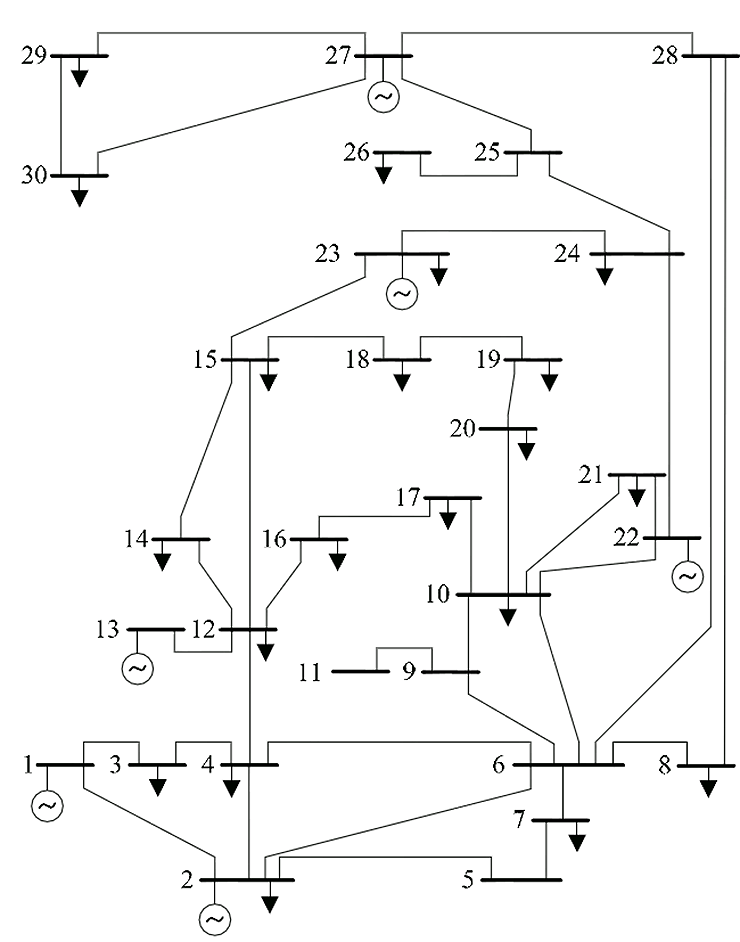
Figure 2: Modified IEEE 30-bus system from Christie (2000).

Since we did not set multi demands for each bus, this indicates $|\mathcal{D}|=|\mathcal{N}|$, and (7b) is going to be an overdetermined system. Therefore our implementation focus on the other three relax versions of AO2 mentioned in Remark 1.

5.2 Numerical Comparison

In this section, we show the comparison of Algorithm (1) with different variations of AO2. Note that all the variations consist inequality constraints $\eqref{eq: relaxed constraints},\eqref{eq: BL},\eqref{eq: UL}$, and the only difference are the objectives, a) Mixed: (7a), b) Relaxed I: $\sum_{k\in\mathcal{D}}y_{k}^{2}r_{k}p^{d}_{k}-\rho\phi(y)$ , c) Relaxed II: $\sum_{k\in\mathcal{D}}y_{k}^{2}r_{k}p^{d}_{k}-\rho\nabla\phi(\tilde{y})^{\top}y$.

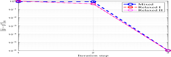
Figure 3: Convergence of $y$ with three variations of AO2.

Figure (3) and Figure (4) shows the convergence of the switch variable $y$ and the complementarity satisfaction $\phi(y)$ respectively. It can be seen that even if the dimension of $y$ is $30$, all the variations of SBQP can converge to the given complementarity tolerance in only a few steps but converge to different solutions. This shows completely different properties than the B$\&$B based solvers.

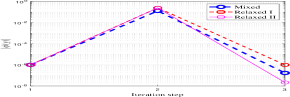
Figure 4: Convergence of $\phi(y)$ with three variations of AO2.

Table 1: Convergence Comparison

Method	Mixed	Relaxed I	Relaxed II
$|\phi(y)|$	1.7e-07	1.0e-06	2.2e-08
Time(s)	0.021	0.046	0.019
Iteration	2	2	2

Table 1 shows the comparison among complementarity satisfaction, operation time and iteration by using different variations. It can be seen that all indicators of the three methods are similar which is different from the results seen in Zhu and Du (2022). Since the three relaxation variations in this paper decrease the number of inequality constraints in AO2 that induce it easier to solve. Notice that, due to the nonlinear structure of (3a), the implementation is more complex than (2a), therefore only AO1 benefits from the reformulation of (3a).

Table 2: Performance Comparison

Method	Mixed	Relaxed I	Relaxed II
Objective	5.421	2.428	5.877
$\sum\limits_{k\in\mathcal{D}}y_{k}p_{k}^{d}$ (p.u.)	1.567	0.825	1.592
$\sum\limits_{k\in\mathcal{D}}y_{k}q_{k}^{d}$ (p.u.)	0.702	0.347	0.709

Table 2 shows the comparison of final performance comparison by using different methods. As can be seen, different variations converge to different local optimum. At least in this case, Relaxed II gets a bit better performance than the other two and Relaxed I is a bit conservative. Note that, both Table 1 and Table 2 show the benefits of the approximate BQP method (Mixed and Relaxed II).

Table 3: Optimal Power Inputs

Bus $\#$	1	2	13	22	23	27
pg (p.u.)	0.400	0.400	0.134	0.250	0.150	0.275
qg (p.u.)	-0.037	0.161	0.213	0.246	0.070	0.125

Table (3) shows the numerical result of optimal system inputs by using Relaxed II based Algorithm (1). The active demands relate with bus $\{$1,2,4,9,10,11,12,13,14,16,17,18,
21,22,23,24,25,26,30$\}$.

6 Conclusion

In this paper, we proposed an effective and fast convergence method named AO-SBQP to optimize microgrid demand shut-offs problems. Importantly, local convergence theory of approximate BQP has been proposed. Moreover, a numerical result on modified IEEE 30-bus case study illustrates the potential of AO-SBQP in this area. Different from B$\&$B and SDR, AO-SBQP can achieve a feasible local optimal solution without tree storage structure or matrix variables. Future research will investigate multistage optimal demand shut-offs and time varing priority of single bus-multiple demands on larger case studies. Moreover, the rank evaluating priority of each demand can vary with time. Comparison of accuracy and computation time of B$\&$B and SDR will also be considered.

References

- Abbey et al. (2014) Abbey, C., Cornforth, D., Hatziargyriou, N., Hirose, K., Kwasinski, A., Kyriakides, E., Platt, G., Reyes, L., and Suryanarayanan, S. (2014). Powering through the storm: Microgrids operation for more efficient disaster recovery. IEEE power and energy magazine, 12(3), 67–76.
- Andersson et al. (2019) Andersson, J.A.E., Gillis, J., Horn, G., Rawlings, J.B., and Diehl, M. (2019). CasADi – A software framework for nonlinear optimization and optimal control. Mathematical Programming Computation, 11(1), 1–36. 10.1007/s12532-018-0139-4.
- Bertsekas (1997) Bertsekas, D.P. (1997). Nonlinear programming. Journal of the Operational Research Society, 48(3), 334–334.
- Bliek1ú et al. (2014) Bliek1ú, C., Bonami, P., and Lodi, A. (2014). Solving mixed-integer quadratic programming problems with ibm-cplex: a progress report. In Proceedings of the twenty-sixth RAMP symposium, 16–17.
- Christie (2000) Christie, R. (2000). Power systems test case archive. Electrical Engineering dept., University of Washington, 108.
- Du et al. (2021) Du, X., Engelmann, A., Faulwasser, T., and Houska, B. (2021). Online power system parameter estimation and optimal operation. In In Proceedings of the American Control Conference, New Orleans, USA, 3126–3131.
- Du et al. (2022) Du, X., Engelmann, A., Faulwasser, T., and Houska, B. (2022). Approximations for optimal experimental design in power system parameter estimation. In 2022 IEEE 61st Conference on Decision and Control (CDC), 5692–5697. IEEE.
- Du et al. (2019) Du, X., Engelmann, A., Jiang, Y., Faulwasser, T., and Houska, B. (2019). Distributed state estimation for ac power systems using gauss-newton aladin. In 2019 IEEE 58th Conference on Decision and Control (CDC), 1919–1924. IEEE.
- Du et al. (2020) Du, X., Engelmann, A., Jiang, Y., Faulwasser, T., and Houska, B. (2020). Optimal experiment design for ac power systems admittance estimation. IFAC-PapersOnLine, 53(2), 13311–13316.
- Frank et al. (2012) Frank, S., Steponavice, I., and Rebennack, S. (2012). Optimal power flow: a bibliographic survey i. Energy systems, 3(3), 221–258.
- Hall (2021) Hall, J. (2021). Numerical Methods and Software for Quadratic Programming Problems with Linear Complementarity Constraints. Master’s thesis, University of Freiburg.
- Hall et al. (2021) Hall, J., Nurkanović, A., Messerer, F., and Diehl, M. (2021). A sequential convex programming approach to solving quadratic programs and optimal control problems with linear complementarity constraints. IEEE Control Systems Letters. 10.1109/LCSYS.2021.3083467.
- Hall et al. (2022) Hall, J., Nurkanovic, A., Messerer, F., and Diehl, M. (2022). Lcqpow–a solver for linear complementarity quadratic programs. arXiv preprint arXiv:2211.16341.
- Kody et al. (2022) Kody, A., West, A., and Molzahn, D.K. (2022). Sharing the load: Considering fairness in de-energization scheduling to mitigate wildfire ignition risk using rolling optimization. In 2022 IEEE 61st Conference on Decision and Control (CDC), 5705–5712. IEEE.
- Li and Bo (2010) Li, F. and Bo, R. (2010). Small test systems for power system economic studies. In IEEE PES General Meeting, 1–4.
- Luo et al. (2010) Luo, Z.Q., Chang, T.H., Palomar, D., and Eldar, Y. (2010). Sdp relaxation of homogeneous quadratic optimization: approximation. Convex Optimization in Signal Processing and Communications, 117.
- Monticelli (1999) Monticelli, A. (1999). State estimation in electric power systems: a generalized approach. Springer Science & Business Media.
- Morrison et al. (2016) Morrison, D.R., Jacobson, S.H., Sauppe, J.J., and Sewell, E.C. (2016). Branch-and-bound algorithms: A survey of recent advances in searching, branching, and pruning. Discrete Optimization, 19, 79–102.
- Nocedal and Wright (2006) Nocedal, J. and Wright, S. (2006). Numerical optimization. Springer Science & Business Media.
- Panora et al. (2014) Panora, R., Gehret, J.E., Furse, M.M., and Lasseter, R.H. (2014). Real-world performance of a certs microgrid in manhattan. IEEE Transactions on Sustainable Energy, 5(4), 1356–1360.
- Ralph* and Wright (2004) Ralph*, D. and Wright, S.J. (2004). Some properties of regularization and penalization schemes for mpecs. Optimization Methods and Software, 19(5), 527–556.
- Rhodes et al. (2020) Rhodes, N., Ntaimo, L., and Roald, L. (2020). Balancing wildfire risk and power outages through optimized power shut-offs. IEEE Transactions on Power Systems, 36(4), 3118–3128.
- Zhu (2015) Zhu, J. (2015). Optimization of power system operation. John Wiley & Sons.
- Zhu and Du (2022) Zhu, S. and Du, X. (2022). Alternating direction based sequential boolean quadratic programming method for transmit antenna selection. In 2022 IEEE 61st Conference on Decision and Control (CDC), 7491–7496. IEEE.
- Zimmerman et al. (2011) Zimmerman, R.D., Murillo-Sanchez, C.E., and Thomas, R.J. (2011). Matpower: Steady-state operations, planning, and analysis tools for power systems research and education. IEEE Transactions on Power Systems, 26(1), 12–19.