Interactive Context-Aware Network for RGB-T Salient Object Detection

Abstract

Salient object detection (SOD) focuses on distinguishing the most conspicuous objects in the scene. However, most related works are based on RGB images, which lose massive useful information. Accordingly, with the maturity of thermal technology, RGB-T (RGB-Thermal) multi-modality tasks attain more and more attention. Thermal infrared images carry important information which can be used to improve the accuracy of SOD prediction. To accomplish it, the methods to integrate multi-modal information and suppress noises are critical. In this paper, we propose a novel network called Interactive Context-Aware Network (ICANet). It contains three modules that can effectively perform the cross-modal and cross-scale fusions. We design a Hybrid Feature Fusion (HFF) module to integrate the features of two modalities, which utilizes two types of feature extraction. The Multi-Scale Attention Reinforcement (MSAR) and Upper Fusion (UF) blocks are responsible for the cross-scale fusion that converges different levels of features and generate the prediction maps. We also raise a novel Context-Aware Multi-Supervised Network (CAMSNet) to calculate the content loss between the prediction and the ground truth (GT). Experiments prove that our network performs favorably against the state-of-the-art RGB-T SOD methods.

1 Introduction

Recently, salient object detection (SOD) draws constantly increasing attention in the computer vision field. The purpose of the SOD task is to identify the most salient objects in the scene. It has many applications in computer vision, graphics, and robotics, such as visual tracking 2012-TPAMI-visualtrack , image and video compression 2009-TIP-compression , image segmentation 2011-ICMT-imageseg , etc. Nevertheless, the single modality of RGB images lacks plenty of important information, which may lead to an incomplete understanding of the scenes. As a result, multi-modal research has now been concerned.

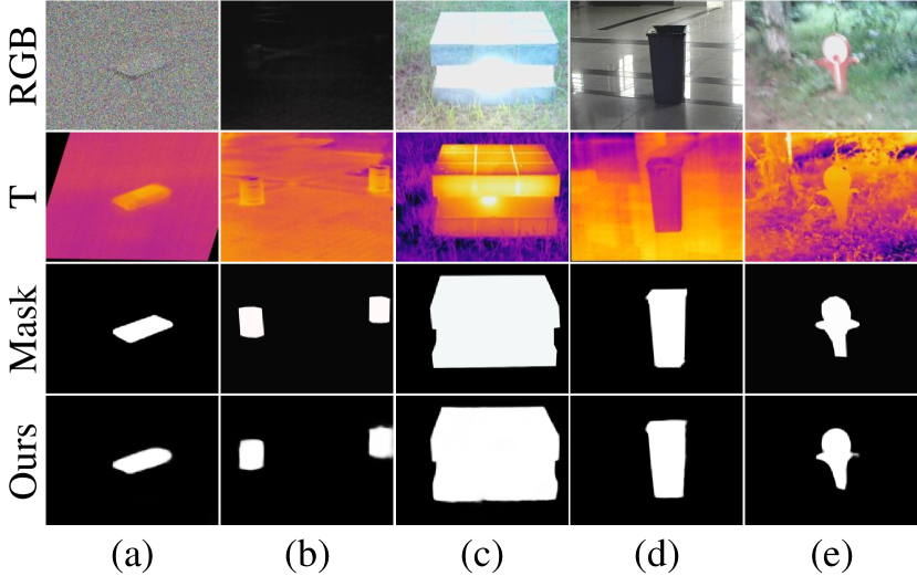
Figure 1: Examples of several challenging scenarios of RGB-T SOD task. (a) Noise; (b) Low illumination; (c) High illumination; (d) Reflection; (e) Mistiness.

For the RGB images, the most obvious shortage is that the depth information is missing, which leads to research on the RGB-D (RGB-Depth) SOD task 2021-TIP-DPANet ; 2021-TNNLS-D3Net ; 2021-CVPR-DCFNet ; 2019-TIP-TANet ; 2020-TIP-ICNet ; 2019-ICCV-DMRA ; 2020-ECCV-CoNet ; 2020-ECCV-DANet ; 2020-CVPR-JL-DCF ; 2020-CVPR-SSF ; 2020-CVPR-UC-Net ; 2020-CVPR-A2dele ; 2021-TIP-CDNet . However, the depth maps can be misleading and are sensitive to light conditions, which makes it difficult to work at night time. Due to the poor robustness of depth sensors, the depth information can be easily disturbed by noise. While with the innovation of thermal sensors, the RGB-T multi-modal research has been constantly explored. Thermal infrared images are less sensitive to light conditions and can be the auxiliary information of the scene. There are numerous applications of thermal sensors. The infrared information helps to identify the surrounding environment in extreme weather conditions. It is also applied in autonomous driving, where semantic segmentation and object detection tasks are mostly applied 2017-IROS-MFNet ; 2020-ICRA-PST900 . Due to the different radiation of different substances, thermal images can indicate distinct features among salient objects and backgrounds. As a consequence, the SOD task is promoted to RGB-T multi-modal field. However, there are still many challenges such as noise interruption. Fig.1 visualizes some examples of challenging scenes.

In this paper, we mainly focus on the RGB-T SOD task and propose a novel neural network called Interactive Context-Aware Network (ICANet). It follows the encoder-decoder architecture. In general, we introduce a useful RGB-T fusion module in the encoder part. In the decoder part, we adopt two cross-scale modules to process the fused features and predict the saliency maps. In the loss function part, we design a multi-supervised network to calculate the content loss besides the traditional loss.

Specifically, we design an RGB-T fusion module called Hybrid Feature Fusion (HFF) module. The term, hybrid feature, means it merges two modalities of features, which are processed by Self-Viewed Perception (SVP) and Self-Scaled Perception (SSP) blocks. SVP uses atrous convolution to gain a larger receptive field. Atrous convolution operation is widely used in detection and segmentation fields 2018-TPAMI-ASPP . Here we adopt different dilated ratios and kernel sizes and organize them into serial to acquire multiple receptive fields. SSP utilizes multiple scales by down-sampling to extract more comprehensive features. These two blocks will process both RGB and thermal features and the output features will be cross-integrated by concatenation operation.

After the cross-modal fusion, we design a Multi-Scale Attention Reinforcement (MSAR) module which aims to interact among the adjacent features. In this module, we adopt the channel and spatial attention mechanism to emphasize the middle-level features 2018-BAM . Subsequently, a simple Upper Fusion (UF) module is implemented to generate the saliency prediction maps of different stages.

In addition, we implement an independent multi-supervised network to calculate content loss along with traditional loss 2021-MSNet . The parameters of the net are initiated with the pre-trained VGG16 model and are weight-locked during the train. The experiment proves it can evaluate the prediction more comprehensively. The net is entitled Context-Aware Multi-Supervised Network (CAMSNet).

Our contribution can be summarized in the following points:

• For the RGB-T SOD task, we propose the HFF module which contains SVP and SSP blocks to implement cross-modal fusion. These two blocks can extract more meaningful information from the original features of a single modality. The HFF module effectively synthesizes the features and integrates them into one output.

• We propose the MSAR module to complete the cross-scale fusion in the decoder part. It is used to integrate the adjacent features to the middle-level feature, which realizes the interaction among different scales of features. Besides, a novel separate multi-supervised neural network (CAMSNet) is designed to calculate the content loss between the prediction and the ground truth (GT).

• Sufficient experiments conducted on 3 RGB-T SOD datasets demonstrate that the proposed method outperforms 15 state-of-the-art methods in terms of six metrics. In addition, experiments on an RGB-D SOD dataset and an RGB-T semantic segmentation dataset demonstrate the universality and effectiveness of the proposed framework.

2 Related work

2.1 RGB Salient Object Detection

Recently, deep learning methods have greatly improved RGB SOD accuracy. Numerous works are proposed based on different emphases. Liu et al. 2019-CVPR-PoolNet proposed a network that utilized pooling operation in convolutional neural networks. Wu et al. 2019-CVPR-MLMNet proposed mutual learning modules to leverage the correlation of multiple tasks and employ foreground contour and edge detection tasks to guide each other. Wu et al. 2019-CVPR-CPD design a novel cascaded partial decoder framework to reduce the complexity of deep aggregation models. Zhao et al. 2019-ICCV-EGNet use edge information to guide the saliency detection. Wei et al. 2020-AAAI-F3Net proposed the cross feature module and cascaded feedback decoder for the task. They also design pixel position-aware loss to assign different weights to different positions in the loss function setting. Pang et al. 2020-CVPR-MINet proposed the aggregate interaction network to integrate the features from adjacent levels.

2.2 RGB-D Salient Object Detection

RGB-D SOD is a typical multi-modal SOD task, in which D means depth information. Multiple deep learning methods have been proposed in recent years. Chen et al. 2021-TIP-DPANet proposed a depth potentiality perception module to avoid contamination of unreliable depth maps and use gated multi-modality attention modules to complete cross-modal fusion. Fan et al. 2021-TNNLS-D3Net proposed a depth depurator unit and a three-stream feature learning module to employ low-quality depth cue filtering and cross-modal feature learning. Ji et al. 2021-CVPR-DCFNet proposed a depth calibration module to calibrate the latent bias in original depth maps.

Although there are many similarities between RGB-T and RGB-D SOD tasks, the detailed implementation still has differences. As a result of the unreliable information on depth images, the spatial structure may confuse the network and lead to bad results. On the other hand, RGB data and thermal data are usually complementary.

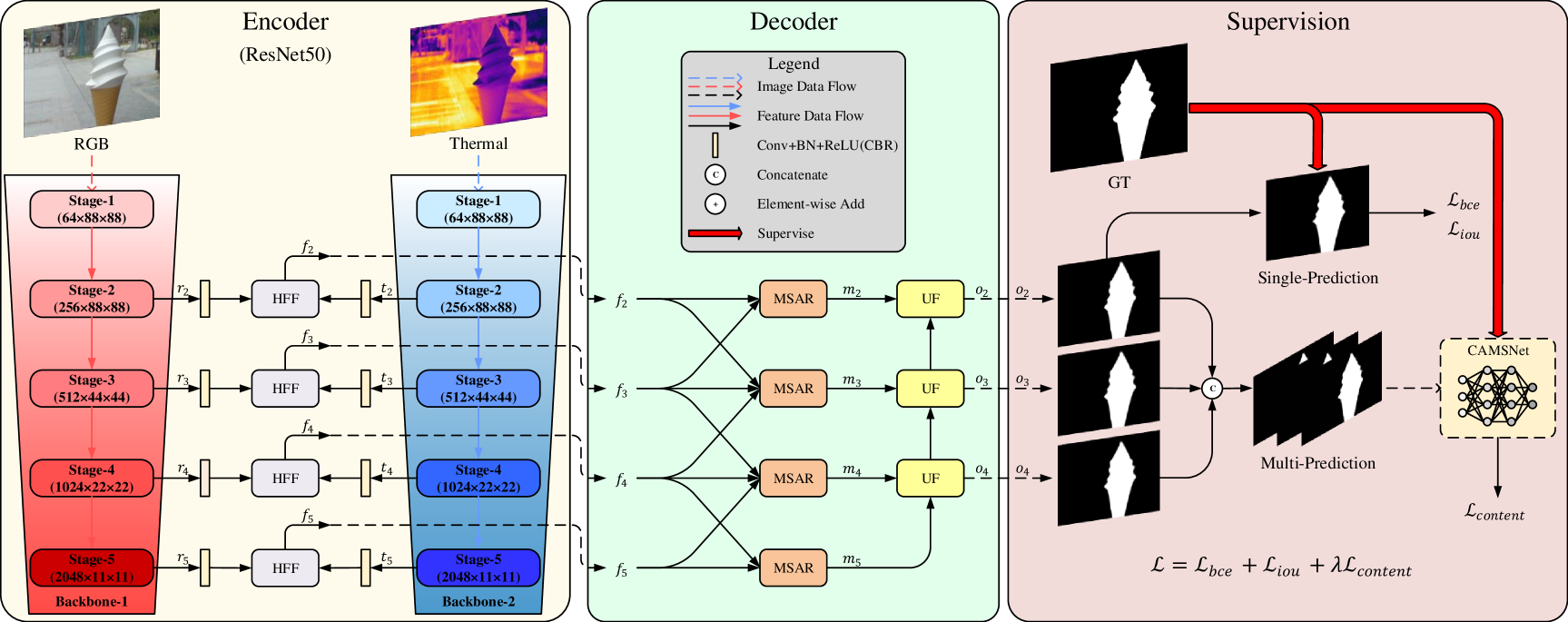
Figure 2: The architecture of ICANet. Considering better visualization effects, we place the details of some modules and blocks in later figures. The network comprises two major parts: Encoder (buff part) and Decoder (green part). The feature flows connect these two parts. The backbones of the encoder part are ResNet50 and VGG16 for final and ablation experiments, respectively. Here takes ResNet50 to illustrate.

2.3 RGB-T Salient Object Detection

With the maturity of thermal technology, the thermal infrared image has reached high resolution and decent quality. Several RGB-T SOD datasets were raised with related algorithms. Wang et al. VT821 proposed the VT821 RGB-T SOD dataset which contains 821 aligned image pairs and provided a graph-based multi-task manifold ranking algorithm. Tu et al. VT1000 constructed another dataset called VT1000 and proposed a collaborative graph learning algorithm. Tu et al. VT5000 contributed to a large-scale dataset VT5000 to explore the robustness of SOD algorithms. They also designed a deep neural network model based on the attention mechanism. The three datasets are the main benchmark datasets in the RGB-T SOD task.

Besides the algorithms proposed with the datasets, some other deep learning methods are proved useful for the task. Tu et al. MIDD proposed a multi-interactive block and a dual-decoder to process the features extracted by the backbone encoder of both RGB and thermal images. Zhang et al. 2020-TIP-FusionCNN utilized different model blocks to implement single-modal fusion, cross-modal fusion, and cross-level fusion respectively. Zhang et al. 2021-TCSVT-HPA based on several DCNN feature fusion strategies proposed a network to learn contextual, complementary, and semantic-aware features.

3 The Proposed Method

3.1 Overall Architecture of ICANet

Fig.2 shows the overall architecture of the proposed network. It consists of two major parts, Encoder and Decoder. The encoder has a symmetric structure that contains parallel backbones. These two independent backbones process the RGB and thermal images simultaneously. In this paper, we choose ResNet50 ResNet and VGG16 VGG as backbones. Fig.2 chooses ResNet50 for illustration. Specifically, we denote the outputs of RGB and thermal branches as $r_{i}(i=2,3,4,5)$ and $t_{i}(i=2,3,4,5)$, respectively. To reduce the computational cost, we utilize the Convolution, Batch Normalization, and ReLU layers (CBR) on the output features to unify the channels to 64. Next the HFF (Sec.3.2) modules fuse these two feature flows into the integrated features $f_{i}(i=2,3,4,5)$. After the RGB-T fusion, the output features $f_{i}(i=2,3,4,5)$ will be fed into the decoder part. The decoder implements cross-scale fusion. $f_{i}(i=2,3,4,5)$ expand branches to the adjacent feature flows and enter the MSAR (Sec.3.3) modules as auxiliary information. There are exceptions for the 2nd-stage and 5th-stage feature flows. Their MSAR modules only have two inputs since they do not have lower or higher features. We indicate the MSAR modules’ output features as $m_{i}(i=2,3,4,5)$. Subsequently, three serial UF (Sec.3.3) modules are set to generate the final prediction results $o_{i}(i=2,3,4)$. The detailed implementation can be checked in the following sections.

3.2 Hybrid Feature Fusion Module

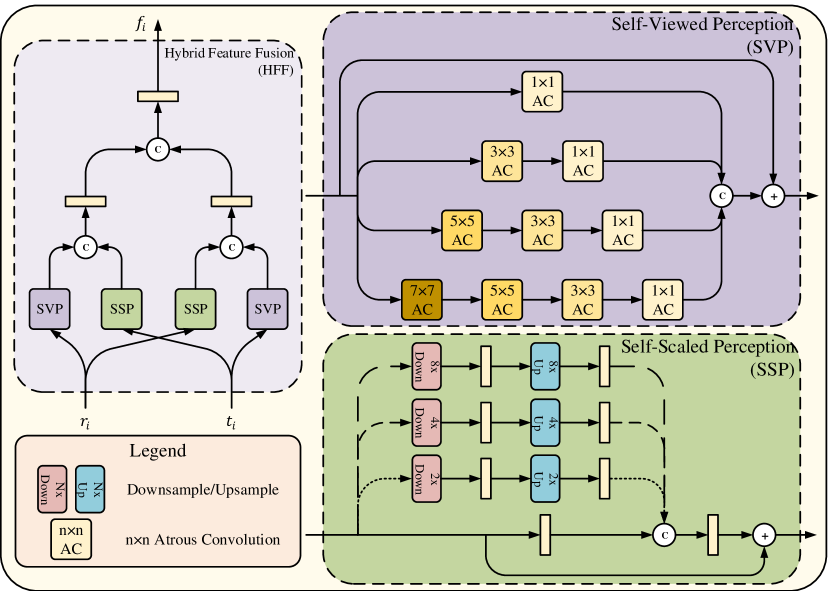
Figure 3: The structure of the HFF module. SVP (purple part) and SSP (green part) blocks are placed on the right. They show the implementation of two feature extraction methods.

The purpose of the Hybrid Features Fusion (HFF) module is to implement cross-modal RGB-T fusion. We design two feature extraction blocks, called Self-Viewed Perception (SVP) and Self-Scaled Perception (SSP), to process the original features from the encoder backbones. Fig.3 shows the structure of the HFF module.

Inspired by 2018-TPAMI-ASPP ; 2018-CVPR-DenseASPP , we adopt atrous convolution to enlarge the receptive field. We choose different kernels with different dilated ratios as branches. The dilated ratios vary from the stages of features and the same sizes share the same dilated ratios. The branch has a serial of the atrous convolution operation. It goes from a larger kernel with a larger dilated ratio to a smaller kernel with a smaller dilated ratio. This particular setting enables features to simultaneously have larger receptive fields and more detailed information. Four branches have different numbers of atrous convolution operations and contain different receptive fields. The outputs of each branch is denoted as $\mathcal{SVP}_{i}(i=1,2,3,4)$. The third branch $\mathcal{SVP}_{3}$ can be represented as an example as follow:

$$\mathcal{SVP}_{3}=\mathcal{AC}_{1}\{\mathcal{AC}_{3}[\mathcal{AC}_{5}(X)]\}$$ (1)

where $X$ represents the input of the block. ${\mathcal{AC}}_{n}(\cdot)$ indicates the atrous convolution (including batch normalization and activation function) and the subscripts represent the kernel sizes.

After the atrous convolution, the features are concatenated directly. The residual structure is used here to avoid degeneration and vanishing gradient problems. The complete process of the SVP block can be indicated as follow:

$$Y=X\oplus({\mathcal{SVP}}_{1}\odot{\mathcal{SVP}}_{2}\odot{\mathcal{SVP}}_{3}\odot{\mathcal{SVP}}_{4})$$ (2)

where $Y$ represents the output of the block. The operators $\oplus$ and $\odot$ denote element-wise addition and concatenation, respectively.

Precious works 2019-CVPR-PAGE ; 2020-PR-U2Net have proposed several methods to down-sample and extract features. SSP block is designed to acquire a better perception of the features by fusing features of different scales. High-level features contain more semantic information while low-level features contain more details. A well-represented feature should combine the benefits of different scale features. Hence, we down-sample the input feature to different scales according to its level. Specifically, we conduct three different ratios of down-sample operations in the second stage while no down-sample operations in the fifth stage. On top of that, a CBR operation is utilized and the features are up-sampled back to the original size by the bi-linear interpolation process. Afterward, the branches’ outputs will be concatenated and a shortcut connection is also used. To illustrate, we take the second stage features as an example to show the steps of the SSP block:

$$\mathcal{SSP}_{1}=\phi(X)$$ (3)

$$\mathcal{SSP}_{2}=\phi\{\mathcal{U}_{2}[\phi(\mathcal{D}_{2}(X))]\}$$ (4)

$$\mathcal{SSP}_{3}=\phi\{\mathcal{U}_{4}[\phi(\mathcal{D}_{4}(X))]\}$$ (5)

$$\mathcal{SSP}_{4}=\phi\{\mathcal{U}_{8}[\phi(\mathcal{D}_{8}(X))]\}$$ (6)

$$Y=X \oplus\phi(\mathcal{SSP}_{1}\odot\mathcal{SSP}_{2}\odot\mathcal{SSP}_{3}\odot\mathcal{SSP}_{4})$$ (7)

where $\mathcal{U}_{n}(\cdot)$ and $\mathcal{D}_{n}(\cdot)$ respectively indicate the up-sample and down-sample operation and the subscripts $n$ are the ratios. $\phi(\cdot)$ represents the CBR operation that was mentioned above.

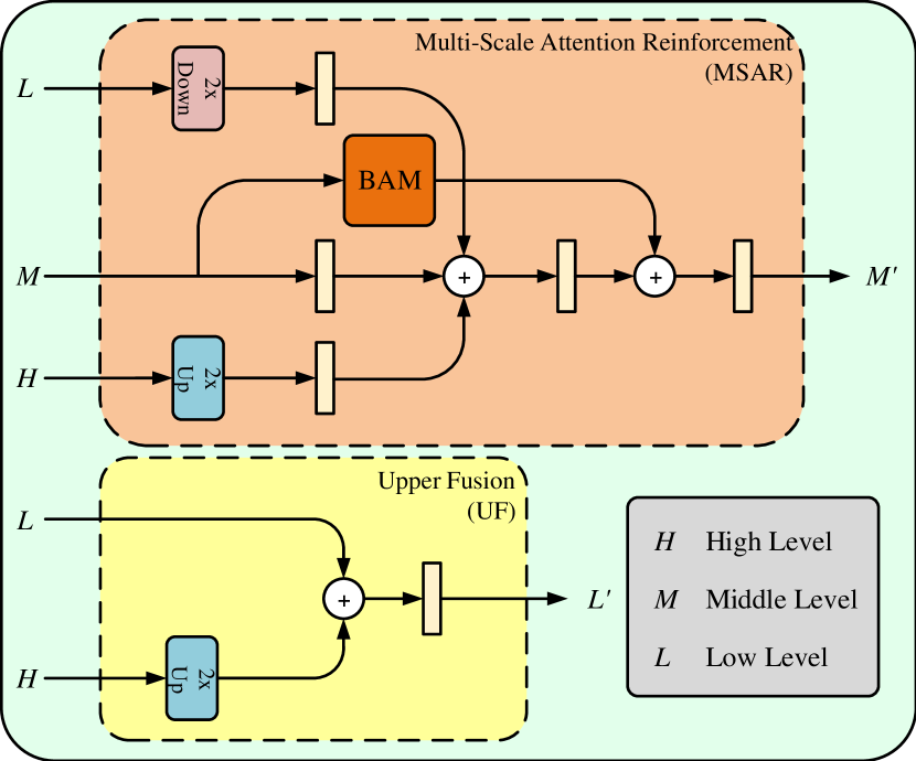
Figure 4: The structure of the decoder part. It contains the MSAR (orange part) and UF (yellow part) modules. The BAM module is utilized in the MSAR module to emphasize the middle-level feature itself.

3.3 Decoder

After the cross-modal fusion, two modules are implemented for cross-scale fusion. As mentioned above, different scales of features contain different information. The method to effectively integrate different levels of features is quite critical. Therefore, we utilize Multi-Scale Attention Reinforcement (MSAR) and Upper Fusion (UF) modules to accomplish it.

Fig.4 denotes the MSAR and UF modules’ detailed pipelines. MSAR module has three different scale input features for the intermediate stages and two for the bilateral stages. It enables different levels of features to interact mutually and scale back to the middle-level stage. We take the three inputs case as an example to demonstrate the whole process. Firstly, the up-sample and down-sample operators are adopted at the high-level and low-level input, respectively. After the CBR operations, these features are added together. To better emphasize the contribution of the middle-level feature, we separate a branch from it. Enlightened by several remarkable works on attention mechanism 2018-BAM ; 2018-ECCV-CBAM ; 2018-CVPR-SE , we try to apply the attention mechanism to better understand features. Experiments prove that BAM 2018-BAM block performs the best. Thus, we append a BAM block at the branch and later add it to the mainstream. The steps above can be represented by the following equations:

$$L^{\prime} =\phi[\mathcal{D}_{2}(L)]$$ (8)

$$H^{\prime} =\phi[\mathcal{U}_{2}(H)]$$ (9)

$$M^{\prime} =\phi(M)$$ (10)

$$M_{a} =\mathcal{BAM}(M)$$ (11)

$$M^{\prime} =\phi[\phi(L^{\prime}\oplus M^{\prime}\oplus H^{\prime})\oplus M_{a}]$$ (12)

where $L,M$, and $H$ are the inputs of the MSAR module and the $M^{\prime}$ is the output. $\mathcal{BAM}(\cdot)$ denotes the BAM attention block. There are exceptions for the 2nd-stage and the 5th-stage of features, for the reason that they do not have the lower and higher features. They only contain two feature inputs and the difference does not affect the structure of the process.

The last procedure of the decoder part is the UF module, which accomplishes the simple up-sample operation and generates the prediction maps. Three UF modules sequentially fuse two features to the lower one. The high-level feature is up-sampled and added to the low-level one. A CBR operation is later utilized. We denote the process by the following formulas:

$$H^{\prime} =\mathcal{U}_{2}(H)$$ (13)

$$L^{\prime} =\phi(L\oplus H^{\prime})$$ (14)

where $L$ and $H$ are the inputs and $L^{\prime}$ is the output of the UF module.

After the decoder part, there will be three output prediction maps labeled $o_{i}(i=2,3,4)$. These results will go to the supervision part to calculate the loss. The 5th output is not under supervision for its resolution is too small.

4 Context-Aware Multi-Supervised Network

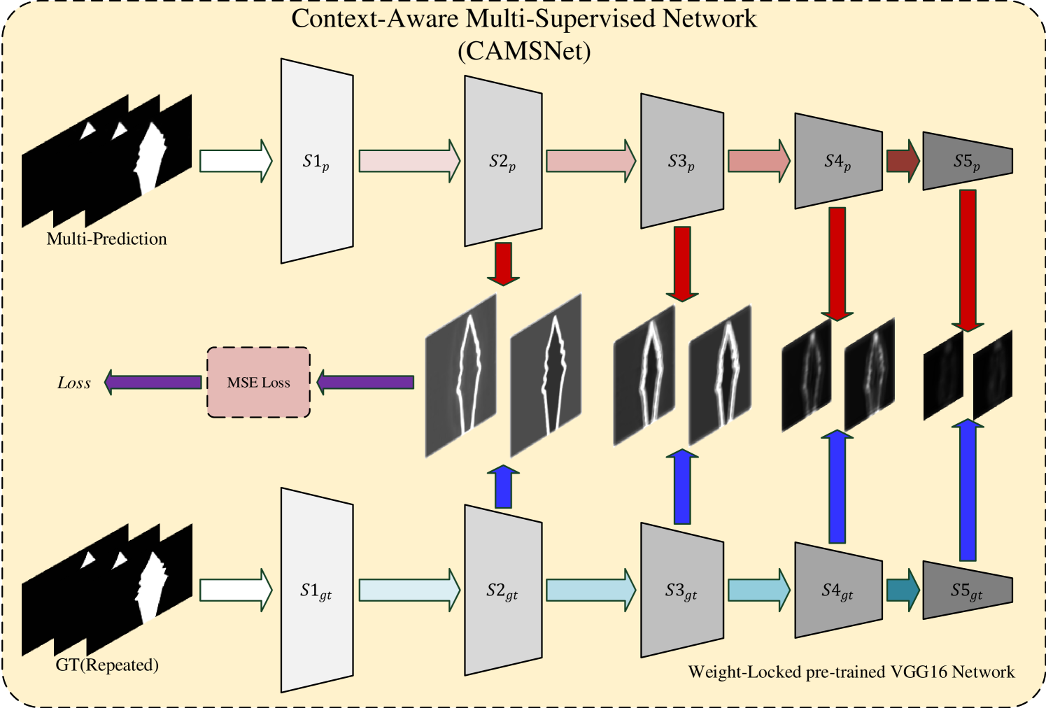
Figure 5: The pipeline of the Context-Aware Multi-Supervised Network (CAMSNet). It is the separate independent net that has a symmetric structure with a weight-locked pre-trained VGG16 network.

The content loss is first applied in the style transfer task. Gatys et al. 2017-CVPR-NS use content loss and style loss as loss functions to measure the difference between content image and style image. Zhao et al. 2021-MSNet alter the idea to the polyp segmentation task. Inspired by these works, we propose the Context-Aware Multi-Supervised Network (CAMSNet) to calculate the content loss between the multi-prediction maps and the GT. As far as we know, this is the first time to apply it for multi-modal saliency detection and multi-modal semantic segmentation tasks.

After three prediction maps are generated, we concatenate them to get a three-channel image. The GT image is repeated two times to get a corresponding three-channel image. These two images will be fed into CAMSNet to calculate the content loss. Fig.5 displays the overall pipeline of CAMSNet. Two images separately flow through the symmetric backbone networks. The backbone is a weight-locked pre-trained VGG16 network, which means it will not upgrade during the training step. Backbones are not limited. We conducted experiments on several common-used backbones such as VGG, ResNet, and PVTv2 2021-ICCV-PVT ; 2022-CVM-PVTv2 . The result shows that VGG16 performs the best, hence we choose VGG16 as the backbone. There are five outputs of the backbone and the 1st-stage feature is omitted. We denote the outputs from the two backbones of prediction and GT as $\mathcal{F}_{i}(i=2,3,4,5)$ and $\mathcal{G}_{i}(i=2,3,4,5)$, respectively. So the content loss $\mathcal{L}_{content}$ can be represented as:

$$\mathcal{L}_{content}=\sum\limits_{i=2}^{5}c_{i}\mathcal{L}_{c}^{i}$$ (15)

where $\mathcal{L}_{c}^{i}(i=2,3,4,5)$ indicate the content loss between $\mathcal{F}_{i}$ and $\mathcal{G}_{i}$. We use mean square error to calculate the difference between two features. It can be represented as:

$$\mathcal{L}_{c}^{i}={\|\mathcal{F}_{i}-\mathcal{G}_{i}\|}^{2}\quad i=2,3,4,5$$ (16)

$c_{i}(i=2,3,4,5)$ are the hyperparameters that adjust the proportion of different stages’ content loss. This is an example visualized in Fig.5. The higher-level features have more semantic information on the location, while the lower-level ones have more details on the edge and boundary. The phenomenon coincides with the theory discussed previously. These four parameters balance the weight of different levels’ content loss. Here we treat them equally and set them all to $1$.

Apart from the CAMSNet loss, we use the binary cross entropy (BCE) and the IoU loss to calculate the basic loss. These can be indicated as follows:

$$\mathcal{L}_{bce} =-\sum\limits_{i=0}^{H}\sum\limits_{j=0}^{W}[Y_{ij}\ln X_{ij}+(1-Y_{ij})\ln(1-X_{ij})]$$ (17)

$$\mathcal{L}_{iou} =1-\frac{\sum_{i=0}^{H}\sum_{j=0}^{W}[Y_{ij}*X_{ij}]}{\sum_{i=0}^{H}\sum_{j=0}^{W}[Y_{ij}+X_{ij}-Y_{ij}*X_{ij}]}$$ (18)

where $X$ and $Y$ are the prediction and GT, respectively. The subscript $ij$ refers to the pixel at the position $(i,j)$.

The total loss function is the addition of the three losses, which can be defined as follows:

$$\mathcal{L}=\mathcal{L}_{bce}+\mathcal{L}_{iou}+\lambda\mathcal{L}_{content}$$ (19)

where $\lambda$ is a hyperparameter that controls the proportion of the content loss. In the experiment, we set $\lambda$ to $0.1$.

5 Experiment

5.1 Experimental Setup

A. Datasets

There are three publicly available benchmark RGB-T SOD datasets, including VT821 VT821 , VT1000 VT1000 , VT5000 VT5000 . They contain the number of image pairs in the corresponding names. The experiment is conducted on these datasets. We use the 2500 pairs of VT5000 as the training set (VT5000-Train) and the remaining part (VT5000-Test) along with VT821 and VT1000 are the testing sets. The RGB-T pairs in the VT821 dataset are manually aligned, thus there are vacant areas in the thermal infrared images. Moreover, the noise is introduced to simulate real environment conditions where images are contaminated and to better improve the robustness. VT1000 contains simple scenes with aligned image pairs in different scenes. VT5000 is the largest and comprises several challenging scenarios.

B. Implementation Details

In the final experiment, the ResNet50 backbone is used to extract RGB and thermal image features. Furthermore, to better validate the performance, we also conduct experiments on the PVTv2 2021-ICCV-PVT ; 2022-CVM-PVTv2 backbone. These two are denoted as ICANet${}^{\text{R}}$ and ICANet${}^{\text{T}}$, respectively. During the training step, the warm-up and linear decay are utilized. The initial learning rates for the backbones and the body are 5e-3 and 5e-2, respectively. The reason for the different settings is that we do not expect the features extracted from the backbone to change sharply. Namely, it is preferable to maintain the feature extraction ability of the backbone and spend more resources on upgrading the body’s parameters. The optimizer is stochastic gradient descent (SGD) with weight decay of 5e-4 and momentum of 0.9. To avoid the overfitting problem, we only train the network 40 epochs with a batch size of 8. The image size is resized to $352\times 352$. The training and testing steps are processed with 128GB RAM and RTX 3080Ti GPU.

C. Model Details

The model speed, parameters, and computational complexity of ICANet are 38.2 FPS, 57.36 M, and 46.92 GMac, respectively.

5.2 Data Augmentation

In our network, we treat the RGB images and thermal images equally. It means each has the same contributions to the results, which may lead to crashes when one in the pair contains contaminated information. Moreover, the thermal images can be easily affected by temperatures, and the RGB images have weak expression abilities under faint illumination scenarios. Additionally, it should be noted that in dataset VT821 VT821 , noises are imposed to simulate real situations. To improve the robustness of our algorithms, we followed the methods proposed by MIDD , applying a data augmentation strategy in the final experiment. Specifically, to solve the former problem, we randomly zero one of the pair modalities by the probability of 5%. For the latter problem, we randomly impose three types of noises into one of the pairs by the probability of 5% as well. The sorts of noises are Gaussian noise, salt and pepper noise, and random noise; and they share the same probabilities to be selected.

5.3 Evaluation Metrics

Table 1: Qualitative comparison of different RGB-T SOD methods. The superscripts V, R, and T indicate VGG16, ResNet50 and PVT backbones, respectively. R+ indicates an extra block is added to the decoder, which can be checked in MIDD . t represents the methods conducted in traditional ways. The best three results are highlighted in red, blue and green. “$-$” denotes that the author does not provide the evaluation results. The arrows $\uparrow$ (or $\downarrow$) of the metrics indicate the value is higher (or lower) the result is better.

Model	VT821				VT1000				VT5000-Test
	$wF$$\uparrow$	$E_{m}$$\uparrow$	$S_{m}$$\uparrow$	MAE$\downarrow$	$wF$$\uparrow$	$E_{m}$$\uparrow$	$S_{m}$$\uparrow$	MAE$\downarrow$	$wF$$\uparrow$	$E_{m}$$\uparrow$	$S_{m}$$\uparrow$	MAE$\downarrow$
MTMR${}^{\text{t}}$${}_{\text{2018-IGTA}}$	.462	.815	.725	.108	.485	.836	.706	.119	.397	.795	.680	.114
M3S-NIR${}^{\text{t}}$${}_{\text{2019-MIPR}}$	.407	.859	.723	.140	.463	.827	.726	.145	.327	.780	.652	.168
SDGL${}^{\text{t}}$${}_{\text{2020-TMM}}$	.583	.847	.765	.085	.652	.856	.787	.090	.559	.824	.750	.089
DMRA${}_{\text{2019-ICCV}}$	.546	.714	.666	.216	.699	.820	.784	.124	.492	.687	.659	.184
S2MA${}_{\text{2020-CVPR}}$	.702	.845	.830	.081	.850	.925	.921	.029	.734	.873	.855	.055
PFA${}_{\text{2019-CVPR}}$	.526	.756	.761	.096	.635	.809	.813	.078	.498	.737	.748	.099
R3Net${}_{\text{2018-IJCAI}}$	.656	.803	.782	.081	.831	.903	.886	.037	.703	.856	.812	.059
BASNet${}_{\text{2019-CVPR}}$	.716	.856	.823	.067	.861	.923	.909	.030	.742	.878	.839	.054
PoolNet${}_{\text{2019-CVPR}}$	.573	.811	.788	.082	.690	.852	.849	.063	.570	.809	.788	.080
CPD${}_{\text{2019-CVPR}}$	.686	.848	.818	.079	.844	.931	.907	.031	.748	.897	.855	.046
EGNet${}_{\text{2019-ICCV}}$	.656	.858	.829	.063	.815	.924	.909	.033	.710	.889	.853	.051
ADF${}_{\text{2022-TMM}}$	.625	.845	.810	.077	.800	.922	.909	.034	.721	.891	.863	.048
MIDD${}^{\text{V}}$${}_{\text{2021-TIP}}$	.759	.898	.871	.045	.856	.942	.915	.027	.762	.900	.867	.043
MIDD${}^{\text{R}}$${}_{\text{2021-TIP}}$	-	.882	.871	.047	-	.927	.921	.025	-	.896	.874	.044
MIDD${}^{\text{R+}}$${}_{\text{2021-TIP}}$	-	.882	.870	.049	-	.929	.921	.027	-	.900	.874	.044
ICANet${}^{\text{R}}$ (Ours)	.804	.908	.884	.032	.887	.945	.927	.021	.803	.916	.875	.037
ICANet${}^{\text{T}}$ (Ours)	.856	.934	.907	.027	.904	.957	.932	.019	.843	.933	.895	.030

Four widely used evaluation metrics are used to judge the models performance, including MAE, wF, S-measure, and E-measure. The PR curve is used to indicate the relation between the precision and recall with a threshold. They can be expressed as the following equations:

$$precision =\frac{TP}{TP+FP}$$ (20)

$$recall =\frac{TP}{TP+FN}$$ (21)

where $TP,FP$, and $FN$ are from the confusion matrix.

Mean Absolute Error MAE (MAE) calculates the mean absolute error between the prediction saliency maps and the GT at the pixel level. The formula is expressed as follows:

$$MAE=\frac{1}{H\times W}\sum_{i=1}^{H}\sum_{j=1}^{W}\lvert S(i,j)-G(i,j)\rvert$$ (22)

where $(H,W)$ is the size of the image. $S(\cdot)$ and $G(\cdot)$ represent the saliency prediction map and the GT map respectively.

F-measure F-measure ($\textbf{F}_{\textbf{m}}$) is used to better evaluate the performance by precision and recall. It can be expressed as follow:

$$F_{m}=\frac{(1+\beta^{2})\cdot precision\cdot recall}{\beta^{2}\cdot precision+recall}$$ (23)

where $\beta^{2}$ is set to 0.3.

Weighted F-measure (wF) is a modified version of F-measure with a weight $w$. The expression is slightly different:

$$wF=\frac{(1+\beta^{2})\cdot precision^{w}\cdot recall^{w}}{\beta^{2}\cdot precision^{w}+recall^{w}}$$ (24)

S-measure S-measure ($\textbf{S}_{\textbf{m}}$) is a spatial similarity evaluation metrics. It can be represented by the equation:

$$S_{m}=\alpha S_{o}+(1-\alpha)S_{r}$$ (25)

where $\alpha$ is set to $0.5$. The $S_{o}$ and $S_{r}$ denote the object-aware and region-aware structural similarities respectively.

E-measure E-measure ($\textbf{E}_{\textbf{m}}$) is the enhanced alignment measure considering both pixel-level and image-level statistic information. It can be quantified as:

$$E_{m}=\frac{1}{H\times W}\sum_{i=1}^{H}\sum_{j=1}^{W}\varphi_{FM}(i,j)$$ (26)

where $\varphi_{FM}$ is the enhanced alignment matrix.

5.4 Comparison with State-of-the-Art Methods

A. Quantitative Evaluation

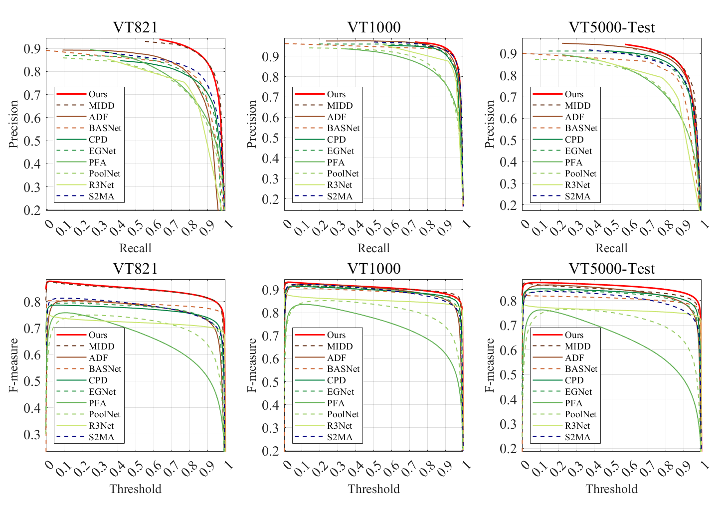
Figure 6: PR curves and F-measure curves with different thresholds on three datasets.

In order to verify the performance of our network, we compare it with other 13 state-of-the-art (SOTA) RGB-T SOD algorithms, including MTMR VT821 , M3S-NIR 2019-MIPR-M3S-NIR , SDGL VT1000 , ADF VT5000 , DMRA 2019-ICCV-DMRA , S${}^{\text{2}}$MA 2020-CVPR-S2MA , MIDD MIDD , PFA 2019-CVPR-PFA , R3Net 2018-IJCAI-R3Net , BASNet 2019-CVPR-BASNet , PoolNet 2019-CVPR-PoolNet , CPD 2019-CVPR-CPD , EGNet 2019-ICCV-EGNet . Tab.1 shows the complete data of all the previous SOTA methods and our proposed network (ICANet). Fig.6 shows the PR curves and F-measure curves. Some of the algorithms are not originally designed for the RGB-T SOD task. For those RGB-D algorithms, we directly transfer them into the RGB-T task as a result of the depth images and thermal images being similar in form. For the remaining single-modal methods, we follow the MIDD method to simply do the early fusion to solve the cross-modal fusion problem. The result shows that our network performs the best in all the evaluation metrics.

Furthermore, it should be emphasized that ICANet is trained for only 40 epochs on GPU, which is considerably low in SOD tasks. Compared to 100 for MIDD , our algorithm has higher efficiency and convergence speed.

B. Qualitative Evaluation

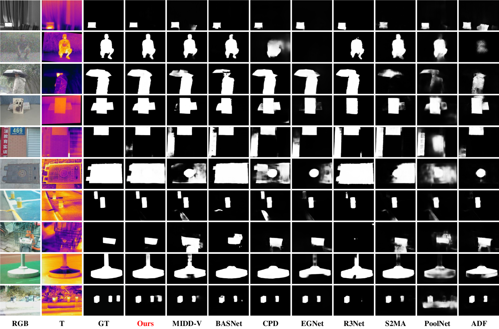
Figure 7: Qualitative comparison among several SOTA algorithms.

Besides the quantitative evaluation, Fig.7 shows the visualization examples. Some of the typical saliency prediction cases are displayed to evaluate the performance. We compare our methods with several previous well-performed SOTA algorithms to show the effectiveness of ICANet.

5.5 Ablation Study

Furthermore, we conduct the ablation experiment to prove the effectiveness of each component in ICANet. Different from the final network, we choose the VGG16 as the backbone to conduct the ablation experiment instead of ResNet50. The detailed results refer to Tab.2.

Specifically, we disassemble the integrated net into scattered parts. SVP, SSP, and MSAR modules are separated to do the module ablation. The reason we omit the UF block is that it is used to up-sample and generate the saliency maps, which can be considered as the FPN 2017-CVPR-FPN operation. It should be noted that we split the HFF module into SSP and SVP blocks, hence choosing both SSP and SVP is equal to the HFF module. Apart from the module ablation, we also conduct the supervision methods ablation to verify the effectiveness of the CAMSNet.

The result proves that our blocks and modules are effective on the task and the integral network performs nearly the best in the ablation experiment.

Table 2: Ablation experiment of our network. The first row contains no modules or blocks, thus it is regarded as the baseline. The best result is highlighted in red.

Model				VT5000
SSP	SVP	MSAR	CAMSNet	$wF$$\uparrow$	$E_{m}$$\uparrow$	$S_{m}$$\uparrow$	MAE$\downarrow$
				.728	.879	.831	.052
✓				.744	.886	.842	.048
	✓			.751	.891	.845	.046
✓	✓			.758	.895	.850	.045
✓	✓	✓		.774	.900	.858	.042
✓	✓	✓	✓	.777	.905	.855	.041

5.6 Experiment on RGB-D SOD Datasets

Apart from the RGB-T SOD task, RGB-D is also a typical form of multi-modality, and they show massive similarities in network structure and data structure. To better illustrate the effectiveness of our network, we conduct experiments on several RGB-D SOD benchmark datasets.

A. Datasets

NJU2K NJU2K contains 1985 image pairs with GT labels collected from the Internet, 3D movies, and photographs. NLPR NLPR contains 1000 image pairs captured by the Microsoft Kinect. The training set combines these two datasets with 1485 pairs from NJU2K (NJU2K-Train) and 700 pairs from NLPR (NLPR-Train).

SIP2021-TNNLS-D3Net is composed of 929 high-resolution image pairs of human activities. STEREOSTEREO consists of 1000 stereoscopic image pairs with the depth images estimated from the stereo images. These two datasets along with the remaining parts of two former datasets (NJU2K-Test and NLPR-Test) are test datasets.

B. Implementation Details

The implementation of the RGB-D experiment is the same as that of RGB-T. The architecture is not changed and the data augmentation strategy is still utilized. All the hyperparameters are set to the same values as the RGB-T experiment.

C. Comparison with Other Methods

Table 3: Qualitative comparison of different RGB-D SOD methods. The best two results are highlighted in red and blue. The arrows $\uparrow$ (or $\downarrow$) of the metrics indicate the value is higher (or lower) the result is better.

Method	STEREO				NJU2K				NLPR				SIP
	$F_{m}$$\uparrow$	$E_{m}$$\uparrow$	$S_{m}$$\uparrow$	MAE$\downarrow$	$F_{m}$$\uparrow$	$E_{m}$$\uparrow$	$S_{m}$$\uparrow$	MAE$\downarrow$	$F_{m}$$\uparrow$	$E_{m}$$\uparrow$	$S_{m}$$\uparrow$	MAE$\downarrow$	$F_{m}$$\uparrow$	$E_{m}$$\uparrow$	$S_{m}$$\uparrow$	MAE$\downarrow$
DF${}_{\text{2017-TIP}}$	.742	.838	.757	.141	.744	.818	.735	.151	.682	.838	.769	.099	.673	.794	.653	.185
CTMF${}_{\text{2017-TC}}$	.771	.870	.848	.086	.779	.864	.849	.085	.723	.869	.860	.056	.684	.824	.716	.139
TANet${}_{\text{2019-TIP}}$	.835	.916	.871	.060	.844	.909	.878	.061	.795	.916	.886	.041	.809	.894	.835	.075
DMRA${}_{\text{2019-ICCV}}$	.762	.816	.752	.086	.872	.921	.886	.051	.855	.942	.899	.031	.815	.858	.800	.088
ICNet${}_{\text{2020-TIP}}$	.865	.915	.903	.045	.868	.905	.894	.052	.870	.944	.923	.028	.836	.899	.854	.069
DCMF${}_{\text{2020-TIP}}$	.841	.904	.883	.054	.859	.897	.889	.052	.839	.933	.900	.035	.819	.898	.859	.068
CoNet${}_{\text{2020-ECCV}}$	.884	.927	.905	.037	.872	.912	.895	.046	.846	.934	.908	.031	.842	.909	.858	.063
DANet${}_{\text{2020-ECCV}}$	.868	.921	.901	.043	.871	.908	.899	.045	.875	.951	.920	.027	.855	.914	.875	.054
JL-DCF${}_{\text{2020-CVPR}}$	.869	.919	.903	.040	.885	.913	.902	.041	.878	.953	.925	.022	.873	.921	.880	.049
SSF${}_{\text{2020-CVPR}}$	.867	.921	.887	.046	.886	.913	.899	.043	.875	.949	.914	.026	.851	.911	.868	.056
UC-Net${}_{\text{20220-CVPR}}$	.885	.922	.903	.039	.889	.903	.897	.043	.890	.953	.920	.025	.868	.913	.875	.051
A2dele${}_{\text{2020-CVPR}}$	.874	.915	.874	.044	.874	.897	.869	.051	.878	.945	.896	.028	.825	.892	.826	.070
S${}^{\text{2}}$MA${}_{\text{2020-CVPR}}$	.835	.907	.890	.051	.865	.896	.894	.053	.853	.938	.915	.030	.854	.911	.872	.057
D${}^{\text{3}}$Net${}_{\text{2021-TNNLS}}$	.859	.920	.899	.046	.865	.914	.901	.046	.861	.944	.912	.030	.835	.902	.860	.063
CDNet${}_{\text{2021-TIP}}$	.873	.922	.896	.042	.866	.911	.885	.048	.848	.935	.902	.032	.805	.880	.823	.076
ICANet${}^{\text{R}}$ (Ours)	.881	.938	.902	.039	.896	.938	.909	.037	.889	.954	.921	.025	.877	.927	.885	.046

We compare our method with 15 other RGB-D SOD algorithms, including DF 2017-TIP-DF , CTMF 2017-TC-CTMF , TANet 2019-TIP-TANet , DMRA 2019-ICCV-DMRA , ICNet 2020-TIP-ICNet , DCMF 2020-TIP-DCMF , CoNet 2020-ECCV-CoNet , DANet 2020-ECCV-DANet , JL-DCF 2020-CVPR-JL-DCF , SSF 2020-CVPR-SSF , UC-Net 2020-CVPR-UC-Net , A2dele 2020-CVPR-A2dele , S${}^{\text{2}}$MA 2020-CVPR-S2MA , D${}^{\text{3}}$Net 2021-TNNLS-D3Net , CDNet 2021-TIP-CDNet . Evaluation metrics are basically the same as RGB-T experiment with a slight difference that F-measure ($\textbf{F}_{\textbf{m}}$) is used instead of weighted F-measure (wF).

Tab.3 shows the quantitative figures of the experiment. We can see that our algorithm reaches decent results and outperforms most other methods, especially on NJU2K and SIP datasets. However, STEREO displays a different pattern. The major reason for the result is that our network treats RGB and thermal information equally, which leads to a high dependency on thermal images. But for depth images, may sometimes mislead the network due to unreliable information. Moreover, the depth images in STEREO datasets are estimated by the stereo images, which have lower accuracy and precision than other datasets. Consequently, the performance on STEREO is unsurprisingly affected.

5.7 Experiment on RGB-T Autonomous Vehicle Semantic Segmentation Dataset

Furthermore, RGB-T SOD can also be applied in the autonomous driving task, for its ability to identify the most remarkable objects in the scenes. To further testify to the universality and learning ability of our method we alter our network to semantic segmentation tasks under autonomous vehicle scenarios.

A. Dataset

MFNet Dataset 2017-IROS-MFNet contains 1569 image-thermal pairs (820 for days and 749 for nights) collected in urban scenes for self-driving systems. It consists of 9 classes (including background) of objects mainly on the roads. Following the experiment of its algorithm, we use the flip strategy in the training step.

Table 4: Qualitative comparison of different semantic segmentation methods on MFNet datasets. The superscript F represents the full RGB-T version of PST900Net. The best two results are highlighted in red and blue. The arrows $\uparrow$ (or $\downarrow$) of the metrics indicate the value is higher (or lower) the result is better.

Method	MFNet Dataset
	Unlabeled	Car	Person	Bike	Curve	Car-Stop	Guardrail	Color-Cone	Bump	mIoU
U-Net${}_{\text{2015-MICCAI}}$	.9690	.6620	.6050	.4620	.4160	.1790	.0180	.3060	.4420	.4510
ERFNet${}_{\text{2017-TITS}}$	.9694	.7384	.6465	.5128	.3773	.1833	.0362	.4023	.4592	.4806
MAVNet${}_{\text{2019-RAL}}$	.8843	.3754	.3975	.1521	.0850	.0240	.0000	.0400	.0440	.2226
Fast-SCNN${}_{\text{2019-arXiv}}$	.9616	.4263	.5141	.4735	.2456	.1087	.0000	.2230	.3462	.3283
MFNet${}_{\text{2017-IROS}}$	.9635	.6154	.5530	.4341	.2231	.0797	.0028	.2088	.2471	.3697
PST900Net${}^{\text{F}}$${}_{\text{2020-ICRA}}$	.9701	.7684	.5257	.5529	.2957	.2509	.0151	.3936	.4498	.4842
ICANet${}^{\text{R}}$ w/o CANet	.9722	.8112	.6059	.5496	.3662	.1861	.0501	.3320	.4297	.4781
ICANet${}^{\text{R}}$ (Ours)	.9724	.8212	.6144	.5572	.3805	.2328	.0307	.3518	.4000	.4846

B. Evaluation Metric

For the semantic segmentation task, the most popular evaluation metric is Intersection-over-Union (IoU). It calculates the proportion of two matrices’ intersection parts and union parts. The average of all classes’ IoUs is called mean IoU (mIoU). It can be indicated by the following equation:

$$mIoU=\frac{1}{n}\sum_{i=0}^{n-1}(\frac{P_{ii}}{P_{ij}+P_{ji}-P_{ii}})$$ (27)

where $n$ denotes the number of all classes (including background (unlabeled), i.e. $i$=0). $P$ indicated the pixel of the prediction map. The subscript $xy$ means class $x$ pixel is predicted as class $y$. Namely, we can also express the equation as follow:

$$mIoU=\frac{1}{n}\sum_{i=0}^{n-1}(\frac{TP}{TP+TN+FP})$$ (28)

In this experiment, we use mIoU as the metric for both datasets.

C. Implementation Details

The implementation of this experiment is different from the original one. We adapt the output channels to the class number of the dataset (i.e. 9) and the CAMSNet part is transferred to the single-supervised one called CANet, which means the input from the prediction map is replaced by the repeated second-level output. The reason for this change is that semantic segmentation tasks usually have multiple classes, which may lead to unstable results of the loss calculation. To calculate content loss, an $argmax$ operation is done in advance to generate the prediction before feeding the output to CANet. Meanwhile, the binary cross entropy loss function is not available here so we change it to a weighted cross entropy loss function. The weight is calculated by the equation $w_{c}=\frac{1}{ln(m+P_{c})}$ proposed by 2016-arXiv-ENet , where the subscript $P_{c}$ denotes the probability of class $c$ and $m$ is a hyperparameter which restricts the range of the weight. Here we use the same value (i.e. $1.02$) as 2016-arXiv-ENet ; 2020-ICRA-PST900 .

The hyperparameters such as learning rate, optimizer, weight decay, momentum, and batch size are the same as our main experiment settings. Two slight differences are that first, we raise our training epoch to 100 because the semantic segmentation tasks are more difficult to train and they have lower convergence speeds. The second difference is the parameter $\lambda$ is set to $0.01$ because multiple classes loss is much higher than weighted cross entropy. Simultaneously, the data augmentation strategy is still activated.

D. Comparison with Other Methods

In this experiment, we evaluate 6 other semantic segmentation algorithms on a self-driving dataset, including ERFNet 2017-TITS-ERFNet , MAVNet 2019-RAL-MAVNet , U-Net 2015-MICCAI-UNet , Fast-SCNN 2019-arXiv-FastSCNN , MFNet 2017-IROS-MFNet , PST900Net 2020-ICRA-PST900 . Meanwhile, we also conduct our experiment without supervision by CANet to demonstrate the effectiveness of the context-aware network in the segmentation task. Except for MFNet and PST900Net, other networks are not specifically proposed for RGB-T tasks. Followed by 2020-ICRA-PST900 , we conduct a simple fusion method to integrate RGB and thermal information.

The result shows that our algorithm outperforms other semantic segmentation methods comprehensively. As a consequence of the different features of different classes, our method is not able to surpass other methods in every class. But we reach almost the best results in nearly all classes, which proves the significance of our work.

6 Conclusions

In this paper, we propose a novel RGB-T SOD network entitled ICANet. We design a multi-modal fusion module called the HFF module using two feature extraction blocks. Then the MSAR module is used to complete the multi-scale fusion with an attention block. Finally, the UF module up-samples the feature streams and generates the saliency prediction maps. Furthermore, we design an independent multi-supervised network called CAMSNet to calculate the content loss between the prediction and GT. The experiment proves that our method performs better than previous SOTA algorithms, and the ablation experiment shows that the modules and blocks are effective for the improvement of saliency prediction. In several other computer vision tasks such as RGB-D SOD and semantic segmentation, the expanded experiment results still prove the effectiveness and versatility of our work.

References

- \bibcommenthead
- (1) Li, J., Levine, M.D., An, X., Xu, X., He, H.: Visual saliency based on scale-space analysis in the frequency domain. IEEE transactions on pattern analysis and machine intelligence, 996–1010 (2012)
- (2) Guo, C., Zhang, L.: A novel multiresolution spatiotemporal saliency detection model and its applications in image and video compression. IEEE transactions on image processing, 185–198 (2009)
- (3) Li, Q., Zhou, Y., Yang, J.: Saliency based image segmentation. In: 2011 International Conference on Multimedia Technology, pp. 5068–5071 (2011)
- (4) Chen, Z., Cong, R., Xu, Q., Huang, Q.: Dpanet: Depth potentiality-aware gated attention network for rgb-d salient object detection. IEEE Transactions on Image Processing, 7012–7024 (2021)
- (5) Fan, D.-P., Lin, Z., Zhang, Z., Zhu, M., Cheng, M.-M.: Rethinking rgb-d salient object detection: Models, data sets, and large-scale benchmarks. IEEE Transactions on Neural Networks and Learning Systems, 2075–2089 (2021)
- (6) Ji, W., Li, J., Yu, S., Zhang, M., Piao, Y., Yao, S., Bi, Q., Ma, K., Zheng, Y., Lu, H., Cheng, L.: Calibrated rgb-d salient object detection, 11
- (7) Chen, H., Li, Y.: Three-stream attention-aware network for rgb-d salient object detection. IEEE Transactions on Image Processing, 2825–2835 (2019)
- (8) Li, G., Liu, Z., Ling, H.: Icnet: Information conversion network for rgb-d based salient object detection. IEEE Transactions on Image Processing, 4873–4884 (2020)
- (9) Piao, Y., Ji, W., Li, J., Zhang, M., Lu, H.: Depth-induced multi-scale recurrent attention network for saliency detection. In: ICCV, pp. 7253–7262 (2019)
- (10) Ji, W., Li, J., Zhang, M., Piao, Y., Lu, H.: Accurate rgb-d salient object detection via collaborative learning. In: European Conference on Computer Vision, pp. 52–69 (2020). Springer
- (11) Zhao, X., Zhang, L., Pang, Y., Lu, H., Zhang, L.: A single stream network for robust and real-time rgb-d salient object detection. In: European Conference on Computer Vision, pp. 646–662 (2020). Springer
- (12) Fu, K., Fan, D.-P., Ji, G.-P., Zhao, Q.: Jl-dcf: Joint learning and densely-cooperative fusion framework for rgb-d salient object detection. In: Proceedings of the IEEE/CVF Conference on Computer Vision and Pattern Recognition, pp. 3052–3062 (2020)
- (13) Zhang, M., Ren, W., Piao, Y., Rong, Z., Lu, H.: Select, supplement and focus for rgb-d saliency detection. In: Proceedings of the IEEE/CVF Conference on Computer Vision and Pattern Recognition, pp. 3472–3481 (2020)
- (14) Zhang, J., Fan, D.-P., Dai, Y., Anwar, S., Saleh, F.S., Zhang, T., Barnes, N.: Uc-net: Uncertainty inspired rgb-d saliency detection via conditional variational autoencoders. In: Proceedings of the IEEE/CVF Conference on Computer Vision and Pattern Recognition, pp. 8582–8591 (2020)
- (15) Piao, Y., Rong, Z., Zhang, M., Ren, W., Lu, H.: A2dele: Adaptive and attentive depth distiller for efficient rgb-d salient object detection. In: Proceedings of the IEEE/CVF Conference on Computer Vision and Pattern Recognition, pp. 9060–9069 (2020)
- (16) Jin, W.-D., Xu, J., Han, Q., Zhang, Y., Cheng, M.-M.: Cdnet: Complementary depth network for rgb-d salient object detection. IEEE Transactions on Image Processing, 3376–3390 (2021)
- (17) Ha, Q., Watanabe, K., Karasawa, T., Ushiku, Y., Harada, T.: Mfnet: Towards real-time semantic segmentation for autonomous vehicles with multi-spectral scenes. In: 2017 IEEE/RSJ International Conference on Intelligent Robots and Systems (IROS), pp. 5108–5115. IEEE, Vancouver, BC (2017)
- (18) Shivakumar, S.S., Rodrigues, N., Zhou, A., Miller, I.D., Kumar, V., Taylor, C.J.: Pst900: Rgb-thermal calibration, dataset and segmentation network. In: 2020 IEEE International Conference on Robotics and Automation (ICRA), pp. 9441–9447. IEEE, Paris, France (2020)
- (19) Chen, L.-C., Papandreou, G., Kokkinos, I., Murphy, K., Yuille, A.L.: Deeplab: Semantic image segmentation with deep convolutional nets, atrous convolution, and fully connected crfs. IEEE Transactions on Pattern Analysis and Machine Intelligence, 834–848 (2018)
- (20) Park, J., Woo, S., Lee, J.-Y., Kweon, I.S.: Bam: Bottleneck attention module. arXiv preprint arXiv:1807.06514 (2018)
- (21) Zhao, X., Zhang, L., Lu, H.: Automatic Polyp Segmentation via Multi-Scale Subtraction Network. arXiv (2021)
- (22) Liu, J.-J., Hou, Q., Cheng, M.-M., Feng, J., Jiang, J.: A simple pooling-based design for real-time salient object detection. In: 2019 IEEE/CVF Conference on Computer Vision and Pattern Recognition (CVPR), pp. 3912–3921. IEEE, Long Beach, CA, USA (2019)
- (23) Wu, R., Feng, M., Guan, W., Wang, D., Lu, H., Ding, E.: A mutual learning method for salient object detection with intertwined multi-supervision. In: 2019 IEEE/CVF Conference on Computer Vision and Pattern Recognition (CVPR), pp. 8142–8151. IEEE, Long Beach, CA, USA (2019)
- (24) Wu, Z., Su, L., Huang, Q.: Cascaded partial decoder for fast and accurate salient object detection. In: 2019 IEEE/CVF Conference on Computer Vision and Pattern Recognition (CVPR), pp. 3902–3911. IEEE, Long Beach, CA, USA (2019)
- (25) Zhao, J., Liu, J.-J., Fan, D.-P., Cao, Y., Yang, J., Cheng, M.-M.: Egnet: Edge guidance network for salient object detection. In: 2019 IEEE/CVF International Conference on Computer Vision (ICCV), pp. 8778–8787. IEEE, Seoul, Korea (South) (2019)
- (26) Wei, J., Wang, S., Huang, Q.: F3net: Fusion, feedback and focus for salient object detection. Proceedings of the AAAI Conference on Artificial Intelligence, 12321–12328 (2020)
- (27) Pang, Y., Zhao, X., Zhang, L., Lu, H.: Multi-scale interactive network for salient object detection. In: 2020 IEEE/CVF Conference on Computer Vision and Pattern Recognition (CVPR), pp. 9410–9419. IEEE, Seattle, WA, USA (2020)
- (28) Wang, G., Li, C., Ma, Y., Zheng, A., Tang, J., Luo, B.: Rgb-t saliency detection benchmark: Dataset, baselines, analysis and a novel approach. In: Image and Graphics Technologies and Applications, pp. 359–369. Springer, Singapore (2018)
- (29) Tu, Z., Xia, T., Li, C., Wang, X., Ma, Y., Tang, J.: Rgb-t image saliency detection via collaborative graph learning. IEEE Transactions on Multimedia, 160–173 (2020)
- (30) Tu, Z., Ma, Y., Li, Z., Li, C., Xu, J., Liu, Y.: Rgbt salient object detection: A large-scale dataset and benchmark. IEEE Transactions on Multimedia, 1–1 (2022)
- (31) Tu, Z., Li, Z., Li, C., Lang, Y., Tang, J.: Multi-interactive dual-decoder for rgb-thermal salient object detection. IEEE Transactions on Image Processing, 5678–5691 (2021)
- (32) Zhang, Q., Huang, N., Yao, L., Zhang, D., Shan, C., Han, J.: Rgb-t salient object detection via fusing multi-level cnn features. IEEE Transactions on Image Processing, 3321–3335 (2020)
- (33) Zhang, Q., Xiao, T., Huang, N., Zhang, D., Han, J.: Revisiting feature fusion for rgb-t salient object detection. IEEE Transactions on Circuits and Systems for Video Technology, 1804–1818 (2021)
- (34) He, K., Zhang, X., Ren, S., Sun, J.: Deep residual learning for image recognition. In: Proceedings of the IEEE Conference on Computer Vision and Pattern Recognition, pp. 770–778 (2016)
- (35) Simonyan, K., Zisserman, A.: Very deep convolutional networks for large-scale image recognition. arXiv preprint arXiv:1409.1556 (2014)
- (36) Yang, M., Yu, K., Zhang, C., Li, Z., Yang, K.: Denseaspp for semantic segmentation in street scenes. In: 2018 IEEE/CVF Conference on Computer Vision and Pattern Recognition, pp. 3684–3692. IEEE, Salt Lake City, UT, USA (2018)
- (37) Wang, W., Zhao, S., Shen, J., Hoi, S.C.H., Borji, A.: Salient object detection with pyramid attention and salient edges. In: 2019 IEEE/CVF Conference on Computer Vision and Pattern Recognition (CVPR), pp. 1448–1457. IEEE, Long Beach, CA, USA (2019)
- (38) Qin, X., Zhang, Z., Huang, C., Dehghan, M., Zaiane, O.R., Jagersand, M.: U2-net: Going deeper with nested u-structure for salient object detection. Pattern Recognition, 107404 (2020)
- (39) Woo, S., Park, J., Lee, J.-Y., Kweon, I.S.: Cbam: Convolutional block attention module. In: Computer Vision – ECCV 2018, pp. 3–19. Springer, Cham (2018)
- (40) Hu, J., Shen, L., Sun, G.: Squeeze-and-excitation networks. In: Proceedings of the IEEE Conference on Computer Vision and Pattern Recognition, pp. 7132–7141 (2018)
- (41) Gatys, L.A., Ecker, A.S., Bethge, M., Hertzmann, A., Shechtman, E.: Controlling perceptual factors in neural style transfer. In: 2017 IEEE Conference on Computer Vision and Pattern Recognition (CVPR), pp. 3730–3738. IEEE, Honolulu, HI (2017)
- (42) Wang, W., Xie, E., Li, X., Fan, D.-P., Song, K., Liang, D., Lu, T., Luo, P., Shao, L.: Pyramid vision transformer: A versatile backbone for dense prediction without convolutions. In: Proceedings of the IEEE/CVF International Conference on Computer Vision, pp. 568–578 (2021)
- (43) Wang, W., Xie, E., Li, X., Fan, D.-P., Song, K., Liang, D., Lu, T., Luo, P., Shao, L.: Pvt v2: Improved baselines with pyramid vision transformer. Computational Visual Media 8(3), 415–424 (2022)
- (44) Perazzi, F., Krähenbühl, P., Pritch, Y., Hornung, A.: Saliency filters: Contrast based filtering for salient region detection. In: 2012 IEEE Conference on Computer Vision and Pattern Recognition, pp. 733–740 (2012). IEEE
- (45) Achanta, R., Hemami, S., Estrada, F., Susstrunk, S.: Frequency-tuned salient region detection. In: 2009 IEEE Conference on Computer Vision and Pattern Recognition, pp. 1597–1604 (2009). IEEE
- (46) Fan, D.-P., Cheng, M.-M., Liu, Y., Li, T., Borji, A.: Structure-measure: A new way to evaluate foreground maps. In: Proceedings of the IEEE International Conference on Computer Vision, pp. 4548–4557 (2017)
- (47) Fan, D.-P., Gong, C., Cao, Y., Ren, B., Cheng, M.-M., Borji, A.: Enhanced-alignment measure for binary foreground map evaluation. arXiv preprint arXiv:1805.10421 (2018)
- (48) Tu, Z., Xia, T., Li, C., Lu, Y., Tang, J.: M3s-nir: Multi-modal multi-scale noise-insensitive ranking for rgb-t saliency detection. In: MIPR, pp. 141–146 (2019)
- (49) Liu, N., Zhang, N., Han, J.: Learning selective self-mutual attention for rgb-d saliency detection. In: Proceedings of the IEEE/CVF Conference on Computer Vision and Pattern Recognition, pp. 13756–13765 (2020)
- (50) Zhao, T., Wu, X.: Pyramid feature attention network for saliency detection. In: Proceedings of the IEEE/CVF Conference on Computer Vision and Pattern Recognition, pp. 3085–3094 (2019)
- (51) Deng, Z., Hu, X., Zhu, L., Xu, X., Qin, J., Han, G.: R3Net: Recurrent residual refinement network for saliency detection. In: IJCAI, pp. 684–690 (2018)
- (52) Qin, X., Zhang, Z., Huang, C., Gao, C., Dehghan, M., Jagersand, M.: Basnet: Boundary-aware salient object detection. In: Proceedings of the IEEE/CVF Conference on Computer Vision and Pattern Recognition, pp. 7479–7489 (2019)
- (53) Lin, T.-Y., Dollar, P., Girshick, R., He, K., Hariharan, B., Belongie, S.: Feature pyramid networks for object detection. In: 2017 IEEE Conference on Computer Vision and Pattern Recognition (CVPR), pp. 936–944. IEEE, Honolulu, HI (2017)
- (54) Ju, R., Ge, L., Geng, W., Ren, T., Wu, G.: Depth saliency based on anisotropic center-surround difference. In: 2014 IEEE International Conference on Image Processing (ICIP), pp. 1115–1119 (2014). IEEE
- (55) Peng, H., Li, B., Xiong, W., Hu, W., Ji, R.: Rgbd salient object detection: A benchmark and algorithms. In: European Conference on Computer Vision, pp. 92–109 (2014). Springer
- (56) Niu, Y., Geng, Y., Li, X., Liu, F.: Leveraging stereopsis for saliency analysis. In: 2012 IEEE Conference on Computer Vision and Pattern Recognition, pp. 454–461 (2012). IEEE
- (57) Qu, L., He, S., Zhang, J., Tian, J., Tang, Y., Yang, Q.: Rgbd salient object detection via deep fusion. IEEE transactions on image processing, 2274–2285 (2017)
- (58) Han, J., Chen, H., Liu, N., Yan, C., Li, X.: Cnns-based rgb-d saliency detection via cross-view transfer and multiview fusion. IEEE transactions on cybernetics, 3171–3183 (2017)
- (59) Chen, H., Deng, Y., Li, Y., Hung, T.-Y., Lin, G.: Rgbd salient object detection via disentangled cross-modal fusion. IEEE Transactions on Image Processing, 8407–8416 (2020)
- (60) Paszke, A., Chaurasia, A., Kim, S., Culurciello, E.: Enet: A deep neural network architecture for real-time semantic segmentation. arXiv preprint arXiv:1606.02147 (2016)
- (61) Romera, E., Alvarez, J.M., Bergasa, L.M., Arroyo, R.: Erfnet: Efficient residual factorized convnet for real-time semantic segmentation. IEEE Transactions on Intelligent Transportation Systems, 263–272 (2017)
- (62) Nguyen, T., Shivakumar, S.S., Miller, I.D., Keller, J., Lee, E.S., Zhou, A., Özaslan, T., Loianno, G., Harwood, J.H., Wozencraft, J., et al.: Mavnet: An effective semantic segmentation micro-network for mav-based tasks. IEEE Robotics and Automation Letters, 3908–3915 (2019)
- (63) Ronneberger, O., Fischer, P., Brox, T.: U-net: Convolutional networks for biomedical image segmentation. In: International Conference on Medical Image Computing and Computer-assisted Intervention, pp. 234–241 (2015). Springer
- (64) Poudel, R.P., Liwicki, S., Cipolla, R.: Fast-scnn: Fast semantic segmentation network. arXiv preprint arXiv:1902.04502 (2019)