Directional superlubricity

How matched/mismatched can two crystalline surfaces be? The geometric conditions for high friction or superlubricity

Design principles for crystalline interfaces: directional locking, directional superlubricity and structural lubricity

Frictionless nanohighways

Frictionless nanohighways and where to find them

Frictionless nanohighways on crystalline surfaces

Abstract

The understanding of friction at nano-scales, ruled by the regular arrangement of atoms, is surprisingly incomplete. Here we provide a unified understanding by studying the interlocking potential energy of two infinite contacting surfaces with arbitrary lattice symmetries, and extending it to finite contacts. We categorize, based purely on geometrical features, all possible contacts into three different types: a structurally lubric contact where the monolayer can move isotropically without friction, a corrugated and strongly interlocked contact, and a newly discovered directionally structurally lubric contact where the layer can move frictionlessly along one specific direction and retains finite friction along all other directions. This novel category is energetically stable against rotational perturbations and provides extreme friction anisotropy. The finite-size analysis shows that our categorization applies to a wide range of technologically relevant materials in contact, from adsorbates on crystal surfaces to layered two-dimensional materials and colloidal monolayers.

I Introduction

When two macroscopically rough surfaces are brought close to each other, they interact only locally at the touching asperities. The progressive increase of touching asperities with load at constant nominal area leads to a contact friction that is proportional to load while independent of area. Contact friction at the atomic scale, on the other hand, follows remarkably different rules Mo et al. (2009); Guerra et al. (2010); Kawai et al. (2016); Liu et al. (2020); He et al. (1999). At small length scales, static friction is largely dependent on the atomic arrangement, and, specifically for crystalline materials, on the mutual relation between the lattice periodicities of the two contacting surfaces. When two atomically flat surfaces come close to each other, the atoms or molecules on one surface can fall into the interatomic gaps of another, leading to an interlocking potential that is strongly dependent on the atomic arrangement at the two contacting surfaces. Such atomic interlocking potentials have strong influences on many nanoscopic frictional processes such as scanning tunneling microscopy experiments Hirano et al. (1997); Feng et al. (2013), nanomanipulations Dietzel et al. (2008); Gigli et al. (2018); Silva et al. (2022) and fabrications of layered two dimensional (2D) materials Novoselov et al. (2016). However, our knowledge of such interlocking effects is incomplete and often obtained in a case-by-case manner, largely due to the material-dependent properties and the complexities of the contacting interfaces such as the contact incommensurabilities and strong finite-size effects.

In an exemplary commensurate contact where the atoms on one surface can perfectly match the inter-atom gaps of the other, interlocking effects are strong as the forces required to unlock individual atoms add up, thus producing a total friction that grows linearly with contact size. On the other hand, when the contacting periodicities are incommensurate, or not perfectly aligned, interlocking forces cancel out, tendentially leading to superlubric sliding or structural superlubricity Hod et al. (2018); Vanossi et al. (2020); Song et al. (2018); Baykara et al. (2018). The relative orientation and directions of motion of a rigid crystalline cluster interacting with an underlying periodic surface were recently shown to be dominated by the possible emergence of common lattice vectors (CLVs) in real and in reciprocal space Cao et al. (2019, 2021). Despite results for specific geometries and potentials de Wijn (2012); Dietzel et al. (2013); Hod (2013), a precise and general quantitative classification of the degree and type of commensurability of contacting lattices and its connection to friction is still currently called for. The present paper aims at filling this gap.

In concrete, we answer the following question: given a crystal-crystal interface that involves two 2D lattices, what kind of ideal frictional behavior can we predict? For a 1D interface, idealized in the Frenkel-Kontorova model Braun and Kivshar (1998), the answer to this question depends on whether the lattice-spacing ratio $a/b$ is rational (high friction) or irrational (superlubric sliding for sufficiently rigid crystals). For the 2D geometry at hand, we classify three very different friction regimes that can arise depending on the (in)commensuration detail in the relation between the two lattices. In between the standard fully commensurate and fully incommensurate conditions, we identify and characterize an intermediate situation, involving an effective 1D-commensuration that produces a finite friction in one direction, but leaves incommensurate superlubric sliding in the perpendicular direction. This condition leads to the “locked” free-sliding direction which in the title we refer to as a frictionless nanohighway, a case of directional structural lubricity. This phenomenon arises when two surfaces lock into a specific orientation, such that static friction vanishes in one specific direction, while remaining finite in all other directions.

Relaxing the condition of infinite size, we obtain theoretical bounds – plus numerical and experimental evidence – of finite-size contacts where approximate versions of each of the infinite-size regimes are realized. In these quasi-commensurate contacts the friction forces along different directions grow as a function of the contact size following very different scaling laws: sublinear and linear in low- and high-friction directions respectively. The emerging anisotropy of friction effectively reproduces the main features of the infinite-size limit also for real-life finite-size contacts.

The results obtained in this paper are derived for rigid lattices. The geometric conditions to differentiate the different friction regimes represents necessary – but possibly not sufficient – conditions for real (i.e. elastic) systems Benassi et al. (2015); Sharp et al. (2016).

II The geometric context

Figure 1: The three types of contacts between two 2D lattices. (a–d) fully commensurate, type A; (e–h) 1D-commensurate, type B; (i–m) fully incommensurate, type C. Panels (a, e, i) display the two contacting lattices in real space: grayscale map of the potential $V_{\mathcal{S}}(\mathbf{r}_{\text{c}})$ with unit-side square-lattice periodicity (black to white = low to high energy); blue dots = adsorbate crystal; orange-edge blue dots = CLVs in real space; light blue arrows = the primitive vectors of the adsorbate lattice. (b, f, j) the corresponding two dual lattices: red dots = adsorbate reciprocal lattice $\mathcal{Q}$; gray dots = substrate reciprocal lattice $\mathcal{G}$; arrows = coincidence vectors (elements of the set $\Omega$). (c, g, k) the linear sum $\mathcal{O}$ of the $\mathcal{R}$ and $\mathcal{S}$ lattices in the Wigner-Seitz cell of the substrate. (d, h, m) the resulting interlocking potential energy (Eq. (2), colorbar at the right) as a function of the adsorbate translation within the substrate Wigner-Seitz cell; for the adopted corrugation potential of Eq. (1), $\tilde{V}_{\mathcal{S}}(\mathbf{0})=-0.0628\epsilon$. The adsorbate lattices are: (a–d) a square lattice with $|a|=\sqrt{5}/3$, and orientation $\theta_{\mathrm{o}}=\tan^{-1}(1/2)$; (e–h) a triangular lattice with $|a|=\sqrt{3/2}$, and orientation $\theta_{\mathrm{o}}=15^{\circ}$; (i–m) a rhombic lattice with primitive vectors of length $|a|=\sqrt{5}/3$ separated by an angle $\psi=1~{}\text{rad}$, with orientation $\theta_{\mathrm{o}}=\text{tan}^{-1}(1/2)$.

We start by recalling a few useful results in the framework of the algebra of reciprocal (dual) lattices, which will allow us to provide a full classification of the contacts between rigid periodic solids.

Consider the problem of moving a monolayer adsorbate crystal across another crystalline surface. Each adsorbate atom interacts with the lateral corrugation potential generated by the underlying crystal surface $V_{\mathcal{S}}(\mathbf{r})$, characterized by the following periodicity: $V_{\mathcal{S}}(\mathbf{r})=V_{\mathcal{S}}(\mathbf{r}+n_{1}\mathbf{S}_{1}+n_{2}\mathbf{S}_{2})$, where $\mathbf{S}_{1}$ and $\mathbf{S}_{2}$ are primitive vectors of the underlying crystal lattice. For example, we construct $V_{\mathcal{S}}$ as

$$V_{\mathcal{S}}(\mathbf{r})=\sum_{n_{1},n_{2}}V(|\mathbf{r}+n_{1}\mathbf{S}_{1}+n_{2}\mathbf{S}_{2}|)$$ (1)

where $V(r)=-\epsilon\exp(-r^{2}/\sigma^{2})$, with $\sigma=0.1\,|\mathbf{S}_{1}|$. Figure 1a,e,i illustrates the crystal overlayered on a square-symmetry substrate potential. The surface forces that contrast the motion of a rigid overlayer result from the gradient of the total (interlocking) potential energy. Its value normalized per monolayer particle is

$$U(\mathbf{r}_{\mathrm{c}})=\frac{1}{N}\sum_{j=1}^{N}V_{\mathcal{S}}(\mathbf{r}_{\mathrm{c}}+\mathbf{R}_{j})\,.$$ (2)

Here $\mathbf{r}_{\mathrm{c}}$ is the center-of-mass displacement and $\mathbf{R}_{j}$ are a set of $N$ lattice-translation vectors, generated as integer linear combinations of two primitive lattice vectors $\mathbf{R}_{1}$ and $\mathbf{R}_{2}$ of the adsorbate. Precisely the list of the $N$ translations defines the contact shape and size.

As derived previously Cao et al. (2019, 2021), in the $N\to\infty$ limit of a macroscopically large perfect crystalline monolayer, the interlocking potential is

$$U(\mathbf{r}_{\mathrm{c}})=\sum_{\mathbf{\Omega}}\tilde{V}_{\mathcal{S}}(\mathbf{\Omega})\exp(i\mathbf{\Omega}\cdot\mathbf{r}_{\mathrm{c}})\,.$$ (3)

Here, the $\mathbf{\Omega}$s are coincidence lattice vectors (CLVs) common to both reciprocal lattices of the monolayer and the periodic surface. $\tilde{V}_{\mathcal{S}}(\mathbf{\Omega})$ are the relevant Fourier components of $V_{\mathcal{S}}(\mathbf{r})$, defined as:

$$\tilde{V}_{\mathcal{S}}(\mathbf{G}):=\frac{1}{A_{\mathcal{S}}}\int_{A_{\mathcal{S}}}V_{\mathcal{S}}(\mathbf{r})\,e^{-i\mathbf{G}\cdot\mathbf{r}}\,\text{d}^{2}\mathbf{r}\,,$$ (4)

where $A_{\mathcal{S}}$ is the area of the primitive cell of $\mathcal{S}$, $i$ is the imaginary unit. Expression (3) is a 2D generalization of the well-known “Poisson summation formula”, $\sum_{n}s(n)=\sum_{k}\tilde{s}(k)$ where $\tilde{s}$ is the Fourier transform of $s$, and the summations run from ${-\infty}$ to ${\infty}$. The dependence of the potential $U(\mathbf{r}_{\mathrm{c}})$ upon the relative orientation of the two contacting lattices enters the expression in Eq. (3) implicitly via the CLVs $\mathbf{\Omega}$.

Notice that the $\mathbf{\Omega}$’s included in the summation have unlimited size. A hypothetical purely sinusoidal potential $V_{\mathcal{S}}({\mathbf{r}})$, as commonly used in friction modeling Gnecco et al. (2001); Fusco and Fasolino (2005); Brazda et al. (2018); de Wijn (2012); Norell et al. (2016), involves few nonzero Fourier components, resulting in few (or even no) non-zero terms in the sum of Eq. (3). In contrast however, our example potential constructed as a sum of Gaussian wells, Eq. (1), involves infinitely many nonzero Fourier components, so that all terms in Eq. (3) are potentially relevant.

The focus of the present paper is how the shape of $U(\mathbf{r}_{\mathrm{c}})$ and the consequent friction phenomenology change (often dramatically), depending on the specifics of the intersection of the reciprocal lattices of the two contacting crystals.

III Algebraic basics

A lattice in $d$ dimension is the set of all vectors obtained as linear combinations with integer coefficients of a set of primitive vectors $\{\mathbf{R}_{1},\mathbf{R}_{2},...,\mathbf{R}_{d}\}$. For the lattice $\mathcal{R}$ generated by this set of primitive vectors we use the following notation:

$$\begin{split}\mathcal{R}&=\left\{\sum_{i}^{d}n_{i}\mathbf{R}_{i}:n_{i}\in\mathbb{Z}\right\}\\ &\stackrel{{\scriptstyle\text{def}}}{{=}}[\mathbf{R}_{1},\mathbf{R}_{2},...,\mathbf{R}_{d}]\,.\end{split}$$ (5)

The dual of an arbitrary set of vectors $\mathcal{R}$ (not necessarily a lattice), indicated by $\hat{\mathcal{R}}$, is defined as the set of all elements $\mathbf{Q}\in\mathbb{R}^{d}$, such that the scalar product $\langle\mathbf{Q},\bm{\rho}\rangle$ is an integer multiple of $2\pi$ for all $\bm{\rho}\in\mathcal{R}$, i.e.

$$\hat{\mathcal{R}}=\left\{\mathbf{Q}:\langle\mathbf{Q},\bm{\rho}\rangle=2\pi k,k\in\mathbb{Z},\forall\bm{\rho}\in\mathcal{R}\right\}.$$ (6)

Note that we include a factor $2\pi$, usually omitted from the standard mathematical definition of a dual. With such convention, the dual of the lattice is its reciprocal lattice.

Let $\mathcal{S}$ be the lattice generated by a second set of primitive vectors $\{\mathbf{S}_{1},\mathbf{S}_{2},...,\mathbf{S}_{d}\}$. The linear sum $\mathcal{S}+\mathcal{R}$ (defined as the set of all sums of one element in $\mathcal{S}$ plus another element in $\mathcal{R}$ of the two lattices is generally not a lattice, but it is a set of vectors, of which we wish to evaluate the dual.

It is a known properties of duals Micciancio and Goldwasser (2002); Micciancio (2010) that $\hat{\mathcal{R}}\cap\hat{\mathcal{S}}=\widehat{\mathcal{S}+\mathcal{R}}$, where $\hat{\mathcal{R}}\cap\hat{\mathcal{S}}$ is the intersection of the individual duals $\hat{\mathcal{S}}$ and $\hat{\mathcal{R}}$.

We adopt the following notation for the $d=2$ problem at hand: the lattice $\mathcal{R}$ and its reciprocal $\mathcal{Q}:=\hat{\mathcal{R}}$ refer to the overlayer crystal; $\mathcal{S}$ and its reciprocal $\mathcal{G}:=\hat{\mathcal{S}}$ refer to the periodic substrate potential. We also indicate the linear sum as $\mathcal{O}:=\mathcal{S}+\mathcal{R}$ and its dual $\Omega:=\hat{O}=\hat{\mathcal{R}}\cap\hat{\mathcal{S}}$. By construction, $\Omega$ is then the set of CLVs in reciprocal space, namely those belonging to both reciprocal lattices $\hat{\mathcal{R}}$ and $\hat{\mathcal{S}}$. For this reason, we will occasionally refer to $\Omega$ as the coincidence set.

Note that any two arbitrary lattices $\mathcal{R}$ and $\mathcal{S}$ can be mapped to a linearly-transformed lattice $\mathcal{R}^{*}$ and a unit square lattice $[\mathbb{1}]$. The explicit isomorphism is $\mathbf{S}^{-1}$ where $\mathbf{S}$ is the matrix whose columns are the vectors $\{\mathbf{S}_{1},\mathbf{S}_{2}\}$ generating $\mathcal{S}$. With this transformation, $\mathcal{S}^{*}=[\mathbb{1}]=[\mathbf{e}_{x},\mathbf{e}_{y}]$, namely the square lattice of unit lattice spacing, and $\mathcal{G}^{*}\equiv\widehat{\mathcal{S}^{*}}$ consists of all reciprocal vectors whose Cartesian components are $2\pi\times$integers. In practice then, to classify the structure of $\mathcal{O}$, one can equivalently focus on $\mathcal{O}^{*}=\mathcal{S}^{*}+\mathcal{R}^{*}$, i.e. the linear sum of the unit square lattice with a properly transformed lattice $\mathcal{R}^{*}=[\mathbf{R}^{*}_{1},\mathbf{R}^{*}_{2}]=[\mathbf{S}^{-1}\mathbf{R}]$.

In the following we stick to the $\mathbf{S}^{-1}$-transformed lattices $\mathcal{R}^{*}$ and $\mathcal{S}^{*}$. For compactness’ sake we omit all stars. Figure 1 already adheres to this convention.

In the next section, we show that three different categories of $\mathcal{O}$ (or its dual $\Omega$) can arise, depending on the mutual (in)commensuration of $\mathcal{R}$ and $\mathcal{S}$. We further show that the specific type of $\mathcal{O}$ pertinent to a given interface between two flat crystalline surfaces bears important implications for the friction exhibited by this interface when the surfaces are set in relative motion.

IV Three categories of commensurability

For a 1D interface, the degree of commensuration is dictated by the ratio $a/b$ between the lattice spacing of the adsorbate and that of the substrate Frenkel and Kontorova (1938); Aubry and Le Daeron (1983); Braun and Kivshar (2004): if this ratio is a rational number, then the two lattices are commensurate; if this ratio is irrational, the lattices are incommensurate. In the rational case the coincidence set $\Omega$ is a 1D lattice where the periodicity is given by the denominator of the ratio. Then the linear-sum space $\mathcal{O}$ is also a discrete set of points repeating along the 1D line, i.e. a 1D lattice. In the irrational case there are no CLVs and $\Omega$ contains the null element only. Hence the sum space $\mathcal{O}$ covers densely the 1D line. For a rigid contact, the rational case has finite friction, while the irrational case is frictionless.

In 2D the linear sum $\mathcal{O}$ is a set of vectors in $\mathbb{R}^{2}$. The friction experienced by the overlayer when it is translated relative to the substrate potential is determined by the geometric mutual commensuration relations of the vectors in $\mathcal{R}$ and $\mathcal{S}$, and their implications for $\mathcal{O}$. These relations characterize how the real plane $\mathbb{R}^{2}$ is covered by the vectors in the sum space $\mathcal{O}$. This coverage occurs in one of three qualitatively different types:

• a sparse coverage by a discrete set of points forming a 2D lattice – Fig. 1c,

• a “comb” coverage by an array of parallel lines – Fig. 1g, and

• a dense area coverage – Fig. 1k.

These geometric alternatives result in three dramatically different patterns of interlocking potential, illustrated in the rightmost column of Fig. 1, and therefore different friction properties. In the following subsections we detail the conditions determining these coverage categories in terms of the reciprocal lattice $\mathcal{Q}=\hat{\mathcal{R}}$ and of the coincidence set $\Omega$.

Type	Condition on the $\mathcal{Q}=\hat{\mathcal{R}}$ lattice	coverage $\mathcal{O}$
A	$\exists\mathbf{Q}_{1},\mathbf{Q}_{2}\in\mathcal{Q}\setminus\{\mathbf{0}\}:Q_{i\mu}/(2\pi)\in\mathbb{Z}\text{ and }\nexists\alpha\in\mathbb{R}:\mathbf{Q}_{1}=\alpha\mathbf{Q}_{2}$	2D discrete
B	$\exists\mathbf{Q}_{1}\in\mathcal{Q}\setminus\{\mathbf{0}\}:Q_{1\mu}/(2\pi)\in\mathbb{Z}$ and $\forall\mathbf{Q}_{2}\in\mathcal{Q}:Q_{2\mu}/(2\pi)\in\mathbb{Z}$, $\exists\alpha\in\mathbb{R}:\mathbf{Q}_{2}=\alpha\mathbf{Q}_{1}$	1D discrete $\otimes$ 1D dense
C	$\nexists\mathbf{Q}\in\mathcal{Q}\setminus\{\mathbf{0}\}:Q_{\mu}/(2\pi)\in\mathbb{Z}$	2D dense

Table 1: The three categories of commensurability, based on how the reciprocal lattice vectors $\mathbf{Q}\in\mathcal{Q}=\hat{\mathcal{R}}$ of the overlayer crystal match the reciprocal $\mathcal{G}=\hat{\mathcal{S}}$ of the substrate unit square lattice.

IV.1 Discrete coverage

Discrete coverage occurs when there exist two linearly independent vectors $\{\mathbf{Q}_{1},\mathbf{Q}_{2}\}$ in the dual $\mathcal{Q}$ of the adsorbate crystal lattice $\mathcal{R}$ such that all components of these vectors are $2\pi\times$ integer numbers, i.e. $Q_{i\mu}/(2\pi)\in\mathbb{Z}$ with $i=1,2$ and $\mu=x,y$. The above condition means that $\mathbf{Q}_{1},\mathbf{Q}_{2}$ exist in $\mathcal{G}$ as well, i.e. $\mathbf{Q}_{1},\mathbf{Q}_{2}\in\Omega=\mathcal{Q}\cap\mathcal{G}$. In this case, summarised in the first row of Table 1, $\Omega$ is a 2D lattice. As a corollary of the above condition, all reciprocal vectors $\mathbf{Q}_{i}\in\mathcal{Q}$ are such that their components $Q_{i\mu}/(2\pi)$ are rational numbers; see Methods Section IX for a proof.

We pick two primitive vectors $\mathbf{\Omega}_{1}$ and $\mathbf{\Omega}_{2}$ of this coincidence reciprocal lattice $\Omega=[{\mathbf{\Omega}}_{1},{\mathbf{\Omega}}_{2}]$, as illustrated in Fig. 1b. The resulting interlocking potential, as expressed in Eq. (3), exhibits a non-vanishing corrugation along both independent directions of ${\mathbf{\Omega}}_{1}$ and ${\mathbf{\Omega}}_{2}$. The interlocking potential energy landscape for the center-of-mass translation takes on a nontrivial shape, such as e.g. the one depicted in Fig. 1d. It can be expressed as

$$U(\mathbf{r}_{\mathrm{c}}) =\sum_{j_{1},j_{2}}\tilde{V}_{\mathcal{S}}(j_{1}\mathbf{\Omega}_{1}+j_{2}\mathbf{\Omega}_{2})\,$$

$$\quad\times\text{exp}\left(i(j_{1}\mathbf{\Omega}_{1}+j_{2}\mathbf{\Omega}_{2})\cdot\mathbf{r}_{\mathrm{c}}\right)\,,$$ (7)

where the sum runs over all integeres $j_{1},j_{2}\in\mathbb{Z}$. Fig. 1d reports this function as resulting from the Fourier components of the potential of Eq. (1). The potential energy landscape reveals a new lattice periodicity, precisely the one emerging in the sum space $\mathcal{O}$, Fig. 1c. In general, this new periodicity is either equal to or shorter than that of the original substrate.

When the monolayer is forced across the periodic surface, it will move more easily along certain directions than along others, due to potential-barrier directional anisotropies. In the example of Fig. 1d, the easy directions are the substrate lattice symmetry directions which avoid the maxima of the energy landscape.

Motion along these preferential directions is usually named directional locking. This phenomenon was observed experimentally in several systems, e.g., for a triangular colloidal crystalline 2D cluster sliding across a triangular substrate Cao et al. (2019, 2021); Bohlein and Bechinger (2012); Korda et al. (2002), for AFM-pushed gold islands on MoS₂ Trillitzsch et al. (2018), and for magnetic vortex lattice under a Lorentz force Villegas et al. (2003), and computationally in different contexts Reichhardt and Nori (1999); Gopinathan and Grier (2004); Frechette and Drazer (2009); Speer et al. (2010); Reichhardt and Reichhardt (2011); Pelton et al. (2004).

IV.2 Line coverage

A second nontrivial condition occurs when the coverage $\mathcal{O}$ is neither discrete nor dense in the whole space. This condition is realized when the dual set $\Omega=\mathcal{Q}\cap\mathcal{G}$ is a 1-dimensional lattice, as in Fig. 1f. In practice, one can identify a nonzero reciprocal lattice vector $\mathbf{Q}_{1}\in\mathcal{Q}$ with the property of having both integer components $Q_{1\mu}/(2\pi)\in\mathbb{Z}$. All other vectors in $\mathcal{Q}$ either are multiples of $\mathbf{Q}_{1}$ or have at least a component divided by $2\pi$ that is an irrational number. Pick one of the two shortest nonzero inversion-symmetric CLV, namely the vectors with the properties of $\mathbf{Q}_{1}$, and call it $\mathbf{\Omega}$. As a result the coincidence set $\Omega$ contains a unique linearly-independent direction, that of $\mathbf{\Omega}$. In other words, $\Omega$ is a 1-dimensional lattice $\Omega=[\mathbf{\Omega}]$, simply the set of all integer multiples of $\mathbf{\Omega}$. When this condition is met, the linear sum space $\mathcal{O}$ is a set of discretely-spaced parallel lines aligned perpendicularly to $\mathbf{\Omega}$, and covered densely in a 1-dimensional sense, see Fig. 1g. This condition is summarised in the second row of Table 1.

In terms of the shortest CLV $\mathbf{\Omega}$, the interlocking potential energy of Eq. (3) becomes:

$$U(\mathbf{r}_{\mathrm{c}})=\sum_{n}\tilde{V}_{\mathcal{S}}(n\mathbf{\Omega})\,\text{exp}(in\mathbf{\Omega}\cdot\mathbf{r}_{\mathrm{c}})\,,$$ (8)

which is the analog of Eq. (IV.1) except now the sum spans the 1D lattice generated by $\mathbf{\Omega}$. As a consequence, the interlocking potential is a function uniquely of the component of the displacement vector $\mathbf{r}_{\mathrm{c}}$ in the $\mathbf{\Omega}$ direction. Explicitly, and importantly, $U(\mathbf{r}_{\mathrm{c}})$ is completely independent of the displacement component of $\mathbf{r}_{\mathrm{c}}$ perpendicular to $\mathbf{\Omega}$. The function $U(\mathbf{r}_{\mathrm{c}})$ can be pictured as a periodic set of parallel straight troughs separated by straight hill ridges, see Fig. 1h. Troughs and ridges are aligned perpendicular to $\mathbf{\Omega}$. As a result, the contact behaves “as commensurate”, and exhibits a finite static friction, in all directions, except for this direction perpendicular to $\mathbf{\Omega}$. In this direction it behaves “as incommensurate” with vanishing static friction, since the through bottom is “flat”, i.e. has a constant energy.

A natural name for this condition is directional structural lubricity.

We are not aware of any previous work where this regime of frictionless nanohighways is hypothesized, nor any existing experiment where this condition was pointed out. In Sec. V.4 below we report its realization in a colloidal experiment, and propose possible heterogeneous contacts between 2D nanomaterials where it should also be accessible.

We realize that in general, if two lattices share the same rotational symmetry of order $n>2$, then there arise either two or no linearly independent CLVs in $\Omega$. Therefore the resulting contact cannot belong to this type B. In Methods Section X we report an argument to illustrate this point.

IV.3 Dense coverage

The final possibility occurs when no nonzero reciprocal lattice vector in $\mathcal{Q}$ exists such that both its components divided by $2\pi$ are integer. This statements amount to say that the coincidence set is $\Omega=\{{\mathbf{0}}\}$, as summarised in the final row of Table 1. The corresponding sum set $\mathcal{O}$ is dense, as shown in Fig. 1k.

The Fourier expansion (3) only includes the null vector: as a result, the interlocking potential energy is perfectly flat

$$U(\mathbf{r}_{\mathrm{c}})=\tilde{V}_{\mathcal{S}}(\mathbf{0})\,,$$ (9)

as in Fig. 1m. No energy is gained or spent in rigidly translating the monolayer by an arbitrary amount in an arbitrary direction. Static friction vanishes. This is the well-known condition of structural superlubricity of fully incommensurate lattices Vanossi et al. (2020); Dienwiebel et al. (2004); Song et al. (2018).

Interestingly, two lattices can even share CLVs in real space, but still have a dense sum space $\mathcal{O}$. This occurs in the example of Fig. 1i–m: these two lattices happen to have infinitely many coincidence points along the substrate direction $\mathbf{S}^{\prime}=(2,1)$, i.e. the intersection $\mathcal{R}\cap\mathcal{S}=[\mathbf{S}^{\prime}]$ (orange-edged blue circles in Fig. 1i). However this real-space intersection is irrelevant to the lubricity of this contact. Instead, the relevant coincidence set $\Omega$ contains only the null vector (Fig. 1j), and, as a result, the 2D linear space is covered densely (Fig. 1k), the average potential energy is flat (Eq. (9) and Fig. 1m), and the static friction vanishes equally in all directions.

V Finite size

The formulas (IV.1)-(9) for the interlocking potential $U(\mathbf{r})$ are valid for an infinite 2D crystalline overlayer interacting with an infinite periodic surface. In practice, however, no contact is infinitely extended. In real-life conditions the overlayer region in contact with the substrate forms a crystalline cluster of finite size $N$. Its finite size and shape do affect the details of the interlocking potential energy $U(\mathbf{r}_{\mathrm{c}})$: in the following, we derive analytical expressions for finite-size contacts and their implications on the frictional behaviour.

As in Eq. (2), we express the position of each particle as a function of the cluster center of mass displacement $\mathbf{r}_{\mathrm{c}}$ and lattice vectors: $\mathbf{r}_{j}=\mathbf{r}_{\mathrm{c}}+\mathbf{R}_{j}$, where precisely the list of the $N$ translations $\mathbf{R}_{j}\in{\mathcal{R}}$ defines the cluster shape and size.

Starting from Eq. (2), we write the explicit expression for the interlocking potential energy $U(\mathbf{r}_{\textrm{c}})$ in terms of the substrate-potential Fourier decomposition.

$$U(\mathbf{r}_{\textrm{c}})= \sum_{\mathbf{G}\in\mathcal{G}}\tilde{V}_{\mathcal{S}}(\mathbf{G})\exp(i\mathbf{G}\cdot\mathbf{r}_{\textrm{c}})$$

$$\times\frac{1}{N}\sum_{j}\exp(i\mathbf{G}\cdot\mathbf{R}_{j})$$ (10)

$$= \sum_{\mathbf{G}\in\mathcal{G}}\tilde{V}_{\mathcal{S}}(\mathbf{G})\exp(i\mathbf{G}\cdot\mathbf{r}_{\textrm{c}})$$

$$\times\frac{1}{N}\sum_{j}\exp(i(\mathbf{G}-\mathbf{Q})\cdot\mathbf{R}_{j})\,,$$ (11)

where $\mathbf{Q}\in\mathcal{Q}$ is an arbitrary vector of the reciprocal lattice of the adsorbate.

In going from Eq. (10) to Eq. (11) we use the property of the reciprocal vectors $\mathbf{Q}$ that $\exp(i\mathbf{Q}\cdot\mathbf{R}_{j})=1\,\forall j$. We take advantage of the freedom in the choice of $\mathbf{Q}\in\mathcal{Q}$ to pick $\mathbf{Q}=\bar{\mathbf{Q}}$ such that $|\mathbf{G}-\bar{\mathbf{Q}}|$ is minimum, and we define

$$\delta\mathbf{\Omega}(\mathbf{G})=\mathbf{G}-\bar{\mathbf{Q}}$$ (12)

to ensure that $\delta\mathbf{\Omega}(\mathbf{G})$ fits in the Wigner-Seitz cell of the adsorbate reciprocal lattice, i.e. in the first Brillouin zone of $\mathcal{R}$. Note how this notation relates with the infinite-size classification of Sec. III: if $\mathbf{G}$ is a common vector between the substrate and adsorbate reciprocal lattices, i.e. $\mathbf{G}\in\Omega$, then $\delta\mathbf{\Omega}(\mathbf{G})=\mathbf{0}$ for that $\mathbf{G}$.

The interlocking potential energy in Eq. (11) now reads

$$U(\mathbf{r}_{\textrm{c}})= \sum_{\mathbf{G}\in\mathcal{G}}\tilde{V}_{\mathcal{S}}(\mathbf{G})\exp(i\mathbf{G}\cdot\mathbf{r}_{\textrm{c}})$$

$$\times\frac{1}{N}\sum_{j}\exp(i\delta\mathbf{\Omega}(\mathbf{G})\cdot\mathbf{R}_{j})$$ (13)

$$= \sum_{\mathbf{G}\in\mathcal{G}}\tilde{V}_{\mathcal{S}}(\mathbf{G})\exp(i\mathbf{G}\cdot\mathbf{r}_{\textrm{c}})\,W(\delta\mathbf{\Omega}(\mathbf{G}),N)\,,$$ (14)

where we defined the weight factor

$$W(\delta\mathbf{\Omega}(\mathbf{G}),N)=\frac{1}{N}\sum_{j}\exp(i\delta\mathbf{\Omega}(\mathbf{G})\cdot\mathbf{R}_{j})\,.$$ (15)

In the following, we omit the explicit dependence of $\delta\mathbf{\Omega}(\mathbf{G})$ on the substrate lattice vector $\mathbf{G}$, $\delta\mathbf{\Omega}=\delta\mathbf{\Omega}(\mathbf{G})$.

Equation (14) expresses the interlocking potential energy $U(\mathbf{r}_{\textrm{c}})$ as a Fourier summation over all the components $\tilde{V}_{\mathcal{S}}(\mathbf{G})$ of the substrate potential Cao et al. (2019). The novelty of finite size compared to Eq. (3) is that the summation of Eq. (14) is not limited to CLVs and it involves the extra size-dependent weight factor defined in Eq. (15).

In the $N\to\infty$ limit, this weight $W(\delta\mathbf{\Omega},N)$ vanishes for those Fourier components with $\delta\mathbf{\Omega}\neq\mathbf{0}$. Therefore, only the $\delta\mathbf{\Omega}=\mathbf{0}$ components determine the overall corrugation of the infinite-size crystal, in agreement with the classification discussed in the previous Section.

At finite size, $W(\delta\mathbf{\Omega},N)$ needs not vanish for any ${\mathbf{G}}$, regardless of whether $\delta\mathbf{\Omega}$ vanishes or not. As a consequence, a priori any Fourier component $\tilde{V}_{\mathcal{S}}({\mathbf{G}})$ of the substrate potential can contribute to the interlocking potential energy $U(\mathbf{r}_{\textrm{c}})$.

In general, the weight $W(\delta\mathbf{\Omega},N)$ is a nontrivial function of $\delta\mathbf{\Omega}$, which depends on the cluster shape. However, for special shapes, analytic expressions for $W(\delta\mathbf{\Omega},N)$ can be derived.

V.1 Special shapes

As a concrete example, consider a parallelogram-shaped cluster of $N$ particles whose particle positions can be expressed as $\mathbf{R}_{j}=j_{1}\mathbf{R}_{1}+j_{2}\mathbf{R}_{2}$, with integer $j_{1},j_{2}=-(\sqrt{N}-1)/2,\dots,(\sqrt{N}-1$)/2, where $\sqrt{N}$ is assumed to be an odd integer, and $\mathcal{R}=[\mathbf{R}_{1},\mathbf{R}_{2}]$. By construction, the cluster center of mass coincides with the particle indexed by $j_{1}=j_{2}=0$. For this cluster shape, the weight function of Eq. (15) can be written as

$$W(\delta\mathbf{\Omega},N) =\frac{1}{N}\sum_{j_{1},j_{2}}\exp(i\delta\mathbf{\Omega}\cdot j_{1}\mathbf{R}_{1})\exp(i\delta\mathbf{\Omega}\cdot j_{2}\mathbf{R}_{2})$$

$$=\frac{1}{N}\frac{\sin(\sqrt{N}\delta\mathbf{\Omega}\cdot\mathbf{R}_{1}/2)}{\sin(\delta\mathbf{\Omega}\cdot\mathbf{R}_{1}/2)}\frac{\sin(\sqrt{N}\delta\mathbf{\Omega}\cdot\mathbf{R}_{2}/2)}{\sin(\delta\mathbf{\Omega}\cdot\mathbf{R}_{2}/2)}\,.$$ (16)

Each factor $f(x)=\sin(\sqrt{N}x/2)/\sin(x/2)$ in Eq. (16) relates to the Fraunhofer diffraction from a narrow-slit grating Born and Wolf (2013). As a function of $x=\delta\mathbf{\Omega}\cdot\mathbf{R}_{i}$, each oscillating factor $f(x)$ peaks at $x=2n\pi$ (for $n\in\mathbb{Z}$), where it reaches its extreme values $(-1)^{n}\sqrt{N}$, i.e. $\pm\sqrt{N}$. As a special consequence, whenever $\delta\mathbf{\Omega}$ vanishes, both fractions becomes equal to $\sqrt{N}$, leading to $W(\delta\mathbf{\Omega},N)=1$: the weight of the corresponding Fourier components in Eq. (14) is independent of size.

The peak width of $f(x)$ is inversely proportional to $\sqrt{N}$, and away from the peaks, say in the intervals $2\pi(n+N^{-1/2})<x<2\pi(n+1-N^{-1/2})$ $f(x)$, oscillates around 0, with values of order 1. As a result, for large cluster size, weights associated to both nonzero $\delta\mathbf{\Omega}\cdot\mathbf{R}_{1}$ and $\delta\mathbf{\Omega}\cdot\mathbf{R}_{2}$ decay as $N^{-1}$. Instead, when just one of these factors vanishes, we expect a nontrivial leading large-size behavior of the associated weight factor, typically as $N^{-1/2}$. These observations account for the leading importance of the Fourier component in the interlocking potential $U(\mathbf{r}_{\mathrm{c}})$ as detailed in the following subsections.

V.2 Coincidence lattice vectors (CLVs)

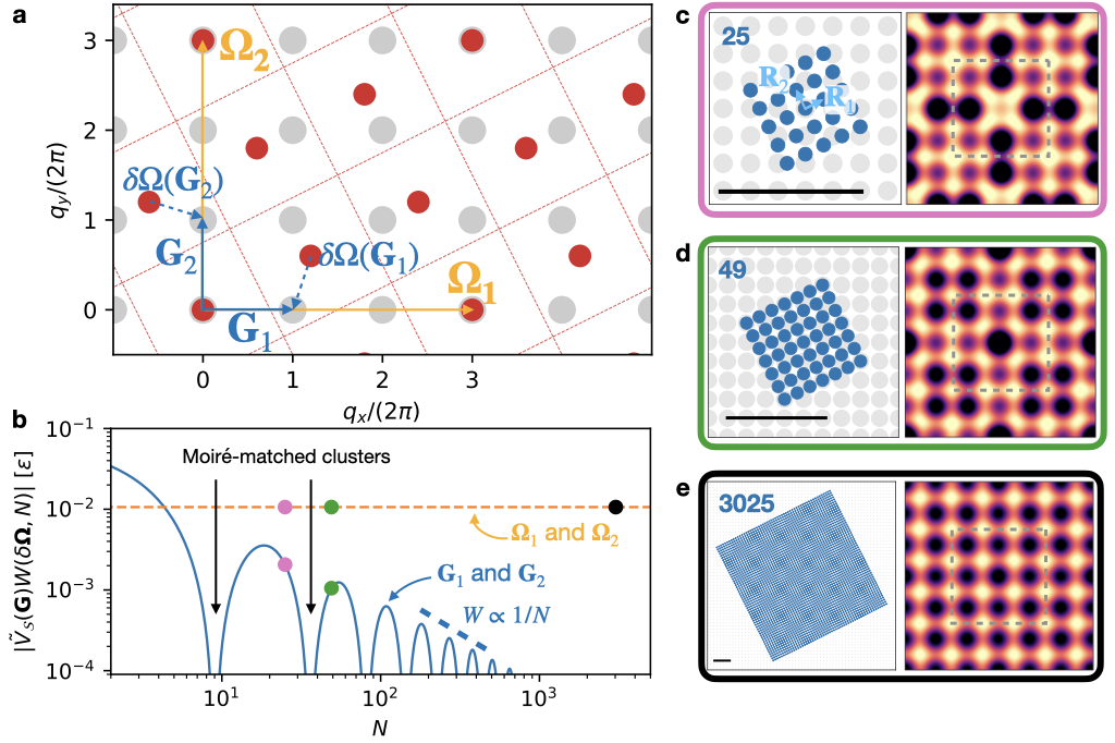
Figure 2: Finite size effects in a contact with discrete coverage. Finite-size analysis for the discrete-coverage (type A) condition in Fig. 1a–d, i.e. a square-lattice adsorbate with $|a|=\sqrt{5}/3$, and orientation $\theta_{\mathrm{o}}=\tan^{-1}(1/2)$. (a) Reciprocal lattices of the adsorbate ($\mathbf{Q}$ points, red dots) and of the substrate ($\mathbf{G}$ points, gray dots); orange arrows highlight two CLVs $\mathbf{\Omega}_{i=1,2}$; blue arrows indicate the substrate primitive vectors $\mathbf{G}_{i}$. Red dashed squares show the first Brillouin zone of the $\mathcal{Q}$ lattice at each lattice point $\mathbf{Q}$. The dashed blue arrows indicate $\mathbf{\delta\Omega}(\mathbf{G}_{i})$, defined in Eq. (12), i.e. the $\bar{\mathbf{Q}}$-translated vectors $\mathbf{G}_{i=1,2}$. Note that $\mathbf{\delta\Omega}(\mathbf{\Omega}_{i})=\mathbf{0}$. (b) The size dependence of the Fourier components $\tilde{V}_{\mathcal{S}}W$ (Eq. (14)) associated with the CLVs $\mathbf{\Omega}_{i}$ (dashed orange line) and for the primitive vectors $\mathbf{G}_{i}$ (solid blue line). The pink, green and black circles mark the cluster sizes $N=25$, $49$, $3025$ of panels (c), (d), and (e), respectively. (c–e) Interlocking potential energy as a function of the cluster center-of-mass position $\mathbf{r}_{\mathrm{c}}$ across the square $[-1,1]\times[-1,1]$ for the displayed clusters. Solid black scalebars in panels (c–e) stand for five lattice spacings. The color scale is the same as in Fig. 1. The gray dashed line highlights the Wigner-Seitz cell of the $\mathcal{S}$ lattice, namely the area shown in Fig. 1d.

When there are CLVs in the dual space, an infinite subset of $\mathcal{G}$ vectors (those belonging to $\Omega$) is associated to vanishing $\delta\mathbf{\Omega}$. For all these terms the weights $W(\delta\mathbf{\Omega},N)$ equal unity, and as a result, the corresponding Fourier components in Eq. (14) contribute as much as for the infinite-size layer, independently of size. All other Fourier components, characterized by nonzero $\delta\mathbf{\Omega}$, can contribute with size-dependent weights. This distinction between size-independent and size-dependent Fourier weights applies to systems with discrete-$\mathcal{O}$ (type-A) and line coverage (type-B) geometries, as discussed for the infinite size-limit in Sec. IV.

Let us focus first on type-A contacts, where two linearly independent CLVs $\mathbf{\Omega}_{1},\mathbf{\Omega}_{2}$, with $\delta\mathbf{\Omega}=\mathbf{0}$, exist. Consider also two non-CLV vectors $\mathbf{G}_{1},\mathbf{G}_{2}$, with $\delta\mathbf{\Omega}\neq\mathbf{0}$, as exemplified in Fig. 2a. It is possible to obtain instructive results for the special parallelogram-shaped clusters introduced in previous section. For $\mathbf{\Omega}_{1,2}$ and $\mathbf{G}_{1,2}$, Fig. 2b reports the Fourier amplitudes $\tilde{V}_{\mathcal{S}}$, modulated by the weights $W$, computed according to Eq. (16). The weight factor $W$ is identically unity at any size for the CLVs (orange dashed line), while it oscillates and decreases as a function of size for non CLVs (blue solid line).

To elucidate the origin of the $\mathbf{G}_{1,2}$-weight oscillations it is convenient to focus on a subset of cluster sizes. Consider the clusters constructed as $\sqrt{N^{\prime}}\times\sqrt{N^{\prime}}$ repetitions of a parallelogram supercell constructed on a pair of independent real-space CLVs $\mathbf{R}^{\text{CLV}}_{1}$ and $\mathbf{R}^{\text{CLV}}_{2}$, namely vectors with all integer components (e.g. the blue orange-edge dots in Fig. 1a). The existence of these real-space CLVs is demonstrated in Methods Section IX. The supercell defined by these (usually non-primitive) vectors contains $K$ vectors and thus the number of particles is $N=KN^{\prime}$. By construction, these special clusters consist of an integer number of identical moiré tiles of $K$ particles in which the relative position of adsorbate and substrate is the same in all repeated units, since $\mathbf{R}^{\text{CLV}}_{1}$ and $\mathbf{R}^{\text{CLV}}_{2}$ belong to the substrate $\mathcal{S}$ lattice too. As a consequence, the average corrugation $U(\mathbf{r}_{\textrm{c}})$ for this class of “moiré-matched clusters” is independent of the number $N^{\prime}$ of moiré patterns in the cluster and coincides with that of the infinite layer. Thus, the only surviving components in Eq. (16) are the CLV with $\delta\mathbf{\Omega}=\mathbf{0}$ that contribute to the corrugation at infinite size: the weight $W$ of any non-CLV vanishes exactly for these “moiré-matched clusters”, as indicated by black arrows in Fig. 2b. The vanishing of $W$ is equivalent to the suppression of the artefact Bragg peaks arising when a non-primitive (e.g., conventional) unit cell is adopted, a well-known feature of the structure factor in crystallography Ashcroft and Mermin (1976), as elaborated in Methods Section XI. This effect was previously noted in realistic crystalline interfaces Koren and Duerig (2016); Wang et al. (2019a): these “moiré-matched clusters” exhibit no size effects, as long as they remain perfectly rigid.

For all other parallelepiped clusters of sizes in between these “moiré-matched clusters”, this cancellation does not occur, leading to $W(\delta\mathbf{\Omega},N)\neq 0$ for non CLVs: the weight function $W$ oscillates as a function of size. $|W|$ reaches a sequence of maxima, whose peak height decays $\propto N^{-1}$ (blue curve in Fig. 2b). Hence the incomplete moiré tiles at the edges result in a size-dependent corrugation, as illustrated in Fig. 2c,d,e.

V.3 Development of directional structural lubricity

Let us now focus on type-B systems, where $\Omega$ is a 1D lattice. The novelty is that a more restricted class of $\delta\mathbf{\Omega}$’s vanishes, and, as a result, the vast majority of the $\mathbf{G}$ vectors in the summation of Eq. (14) lead to size-dependent Fourier contributions.

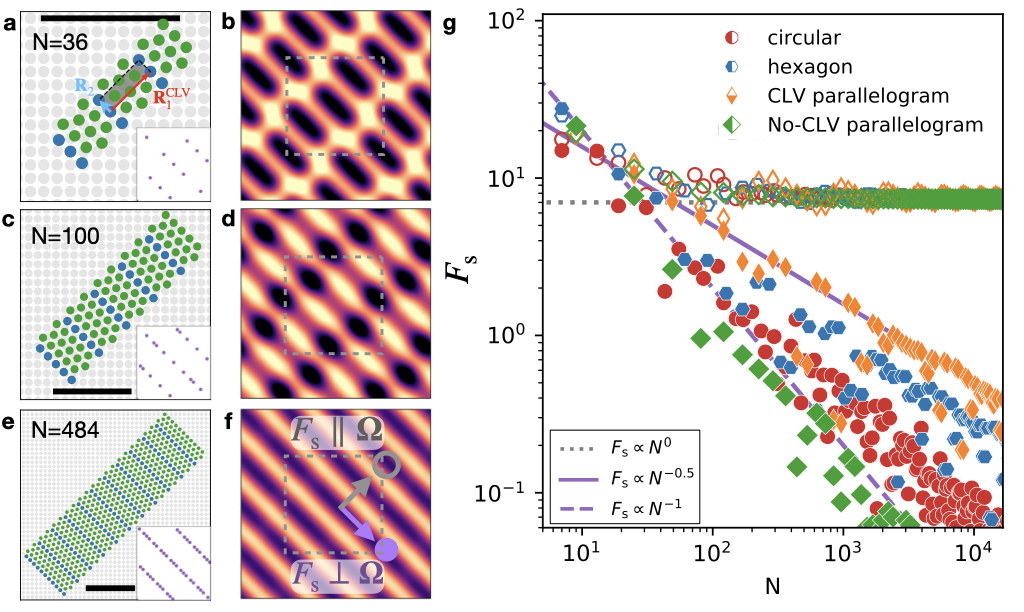
Figure 3: The development of directional structural lubricity with increasing contact size. (a),(c),(e) Adsorbate clusters of different sizes with the same contact incommensurability (type B) as of Fig. 1(e), namely a triangular-lattice adsorbate with spacing $a=\sqrt{3/2}$ and orientation $\theta_{\mathrm{o}}=15^{\circ}$ sliding across a square-lattice substrate with unit lattice spacing. These special-shaped clusters here are constructed by repeating a $K=4$-particle unit (shaded area in panel a) based on a real-space CLV $\mathbf{R}^{\mathrm{CLV}}_{1}$ (red arrow in panel a) and a primitive vector $\mathbf{R}_{2}$ (light-blue arrow in panel a). The corners of the repeated cell are highlighted in blue. The black bar in each panel spans 10 substrate lattice spacings. The insets report the corresponding coverage $\mathcal{O}$ for that given size. (b), (d), (f) The interlocking potential energy of the clusters in (a), (c), (e) respectively as a function of $\mathbf{r}_{\text{c}}\in[-1,1]\times[-1,1]$. The color code is the same as in Fig. 1. The gray dashed line highlights the Wigner-Seitz cell. (g) The cluster-size dependence of static friction for the directionally superlubric interface. Filled (empty) symbols refer to the unpinning force parallel (perpendicular) to the low-energy corridors, or perpendicular/parallel to the CLV $\mathbf{\Omega}$, respectively. These directions are sketched in panel f. The investigated shapes of the clusters (circles, hexagons, parallelograms) are reflected in the data-point shapes and colors (red, blue, and orange/green). Parallelograms are generated by replicating two kinds of supercells: either based on a real-space CLV (orange) or not (green); the adopted supercell lattice vectors are respectively $4\mathbf{R}_{1}+2\mathbf{R}_{2}$ and $2\mathbf{R}_{2}$ (orange), or $2\mathbf{R}_{1}$ and $2\mathbf{R}_{1}+2\mathbf{R}_{2}$ (green), where $\mathbf{R}_{1}$ $\mathbf{R}_{2}$ are identified in Fig. 1e. The dotted, solid, and dashed lines report the $F_{\mathrm{s}}\propto N^{0}$, $F_{\mathrm{s}}\propto N^{-1/2}$, and $F_{\mathrm{s}}\propto N^{-1}$ scalings as guides to the eye.

In the (not guaranteed) circumstance that, beside reciprocal CLVs, we also identify a real-space CLV $\mathbf{R}^{\text{CLV}}_{1}$, we can adopt it as one of the primitive vectors for a supercell. The second supercell primitive vector $\mathbf{R}_{2}$ can be chosen freely among the lattice vectors linearly independent of $\mathbf{R}^{\text{CLV}}_{1}$, e.g. $\mathbf{R}_{2}$ in Fig. 1e. Compared to the discrete-$\mathcal{O}$ condition, here $\mathbf{R}_{2}$ is certainly not a CLV. As in the previous section, such a supercell contains $K$ vectors $\mathbf{R}_{k}$, yielding a cluster of size $N=N^{\prime}K$. See Fig. 3a,c,e for examples of clusters built with this protocol.

For this class of clusters, the first factor in Eq. (16) has $\delta\mathbf{\Omega}\cdot\mathbf{R}^{\mathrm{CLV}}_{1}=0$, and thus $\exp(i\delta\mathbf{\Omega}\cdot\mathbf{R}^{\mathrm{CLV}}_{1})=1$, because $\mathbf{R}^{\mathrm{CLV}}_{1}$ belongs to both the adsorbate and substrate lattice, i.e. $\mathbf{R}^{\mathrm{CLV}}_{1}\in\mathcal{R}\cap\mathcal{S}$. As a result, the second factor leads to a scaling $N^{-1/2}$ for any $\delta\mathbf{\Omega}\neq 0$: the weight is constant for the CLV $\mathbf{\Omega}$ while the envelope of non-CLV weights decays as $N^{-1/2}$.

The corrugation of this system can be expressed as the sum of the size-independent term, namely the $\mathbf{\Omega}$-sum of Eq. (8) (resulting in the corrugation of Fig. 1h), plus the remaining contributions, which decay as a function of size:

$$U(\mathbf{r}_{\textrm{c}}) =\sum_{n}\tilde{V}_{\mathcal{S}}(n\mathbf{\Omega})\exp(in\mathbf{\Omega}\cdot\mathbf{r}_{\textrm{c}})$$

$$+\sum_{\mathcal{G}\textbackslash\Omega}\tilde{V}_{\mathcal{S}}(\mathbf{G})\exp(i\mathbf{G}\cdot\mathbf{r}_{\textrm{c}})W(\delta\mathbf{\Omega},N)\,,$$ (17)

$$W(\delta\mathbf{\Omega},N) \propto K/\sqrt{N}\,.$$

An example of size evolution of the energy landscape resulting from Eq. (17) is reported in Fig. 3b,d,f. For large size, $U(\mathbf{r}_{\textrm{c}})$ approaches the straight and flat energy corridors of Fig. 1h.

The Fourier amplitude of each term in Eq. (17) is the product of the weight $W(\delta\mathbf{\Omega}({\mathbf{G}}),N)$ times the substrate Fourier component $\tilde{V}_{\mathcal{S}}(\mathbf{G})$ evaluated at the same vector $\mathbf{G}$. Assuming, as is usually the case, that the surface corrugation potential $V_{\mathcal{S}}(\mathbf{r})$ is a smooth function, then its Fourier amplitudes $|\tilde{V}_{\mathcal{S}}(\mathbf{G})|$ tend to decay with $|\mathbf{G}|$. As a consequence, long $\mathbf{G}$ vectors even if leading to nearly perfect matching (i.e. small $\delta\Omega(\mathbf{G})$), usually yield quite small, practically negligible contributions to the energy landscape. As a result, the size-dependent term in Eq. (17) is usually dominated by a few small-$|\mathbf{G}|$ Fourier components.

This size-dependent energy corrugation has important implication for friction. In an overdamped context where inertia is negligible, the minimum per-particle force $F_{\mathrm{s}}$ needed to sustain the motion of the adsorbate crystal in a given direction $\hat{\mathbf{u}}$, namely the static friction force $F_{\mathrm{s}}$ in that direction, can be estimated by $\max_{\mathbf{r}_{\mathrm{c}}\in\mathcal{L}}|\hat{\mathbf{u}}\cdot\nabla U({\mathbf{r}}_{\mathrm{c}})|$, where $\mathcal{L}$ is the straight line connecting two successive energy minima in the $\hat{\mathbf{u}}$ direction. In the present type-B condition, if $\hat{\mathbf{u}}$ is aligned along the energy corridors, then only the $\delta\Omega(\mathbf{G})\neq\mathbf{0}$ components contribute, leading to $F_{\mathrm{s}}\propto N^{-1/2}$, whereas if $\hat{\mathbf{u}}$ has a nonzero component perpendicular to the corridors, then $F_{\mathrm{s}}$ contains a leading component $\propto N^{0}$ from the ${\mathbf{G}}\in\Omega$ Fourier components.

We have verified numerically that the same power laws-scaling of $F_{\mathrm{s}}$ holds not just for special-shaped parallelogram clusters, but also for different shapes, as reported in Fig. 3g: similar decays of $F_{\mathrm{s}}$ parallel to the energy corridor are found for each shape. However, it is apparent that, for a given size, different cluster shapes can change the value of this parallel friction component by an order of magnitude. In contrast, the size-independent perpendicular friction component is nearly independent of the cluster shape, too.

These direction-dependent scaling laws justify the name directional structural lubricity for the type-B interface condition: along the energy corridor the total friction $N\,F_{\mathrm{s}}$ scales sublinearly with the cluster size, as in standard structural lubricity, while parallel to these corridors the total friction $N\,F_{\mathrm{s}}$ grows linearly with size, like for a ordinary structurally-matched interface.

V.4 Close-matching vectors

We come now to extend the exact classification of Sect. IV to interfaces which –strictly speaking– belong to type C, but come with a set of relatively short $\mathbf{G}$ vectors characterized by a very small mismatch $|\delta\mathbf{\Omega}(\mathbf{G})|$, see Eq. (12): close-matching vectors (CMVs). This approximate classification holds for finite, and not-too-large clusters.

When the two crystals are incommensurate (type-C), the “standard” properties of structural lubricity should apply. However we argue here that in the presence of CMVs the categories and size scaling introduced above survive, up to a maximum cluster size related inversely to $|\delta\mathbf{\Omega}(\mathbf{G})|$. In this section we focus on directional locking and directional structural lubricity, showing that, in specific size ranges, they are to be expected for type-C interfaces with CMVs. This analysis is especially relevant for heterocontacts, where perfect matches (whether of type A or B) are unlikely.

We recall that, for each substrate Fourier component identified by $\mathbf{G}$, the $N$-dependence of both factors $f(x)$ in Eq. (16) implies a critical size below which $W(\delta\mathbf{\Omega}(\mathbf{G}),N)\simeq 1$ because both $f(x)$ factors in $W$ are of order $N^{1/2}$. For a special-shape cluster (see Section V.1) based on the vectors $\mathbf{R}_{1}$ and $\mathbf{R}_{2}$, the critical size associated with a substrate vector $\mathbf{G}$ is

$$N_{\mathrm{c}}(\mathbf{G})=\left[\min\left(\frac{2\pi}{\delta\mathbf{\Omega}(\mathbf{G})\cdot\mathbf{R}_{1}},\frac{2\pi}{\delta\mathbf{\Omega}(\mathbf{G})\cdot\mathbf{R}_{\mathrm{2}}}\right)\right]^{2},$$ (18)

where the argument of the square is meant to be rounded to the next integer. If the cluster size is $N\lesssim N_{\mathrm{c}}(\mathbf{G})$, then

$$W(\delta\mathbf{\Omega}(\mathbf{G}),N)\simeq 1\,.$$ (19)

Let us assume that there exists a single independent CMV $\mathbf{G}^{\prime}\simeq\mathbf{Q}^{\prime}$ such that, at its critical size $N^{+}=N_{\mathrm{c}}(\mathbf{G}^{\prime})$, $\mathbf{G}^{\prime}$ gives the dominant contribution to the corrugation energy $U(\mathbf{r}_{\mathrm{c}})$ of the contact in Eq. (14). The $\mathbf{G}^{\prime}$ Fourier component becomes the dominating one only beyond some minimum size $N^{-}$, defined as the largest $N<N^{+}$ such that $\exists\mathbf{G}\in\mathcal{G}\setminus\{\pm\mathbf{G}^{\prime}\}$ which satisfies $|\tilde{V}_{\mathcal{S}}(\mathbf{G})W(\delta\mathbf{\Omega}(\mathbf{G}),N)|\geq|\tilde{V}_{\mathcal{S}}(\mathbf{G}^{\prime})W(\delta\mathbf{\Omega}(\mathbf{G}^{\prime}),N)|$.

If the contact conditions are such that $N^{-}$ is significantly smaller than $N^{+}$ then this contact exhibits approximate directional superlubricity for all sizes in the range $N^{-}<N<N^{+}$. In this size range, the direction perpendicular to $\mathbf{G}^{\prime}$ exhibits a very small corrugation associated to minor Fourier components, negligible compared to the $\tilde{V}_{\mathcal{S}}(\mathbf{G}^{\prime})W(\delta\mathbf{\Omega}(\mathbf{G}^{\prime}),N)$ term, which is responsible for a sizeable corrugation in the direction parallel to $\mathbf{G}^{\prime}$. As the size $N$ exceeds $N^{+}$, also this sizeable corrugation perpendicular to the superlubric “corridor” begins to fade away due to the decay of $W(\delta\mathbf{\Omega}(\mathbf{G^{\prime}}),N)$, until “standard” direction-independent structural lubricity of an extended type-C contact is recovered.

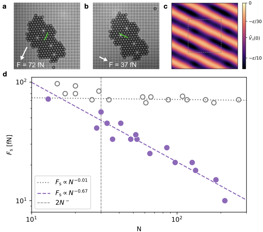
Figure 4: Experimental realisation of directional structural lubricity. (a,b) A triangularly packed colloidal cluster of size $N=185$ with spacing $a=4.45~{}\mu\textrm{m}$ sliding across a square-lattice surface with spacing $b=5.0~{}\mu\textrm{m}$. The green lines in both panels indicate the cluster’s center of mass trajectory (see also movie 1) over a period of 85 seconds under the indicated applied forces perpendicular (a) and parallel (b) to the energy corridor. If the same force strength of 37 fN was applied in the direction of panel (a), the cluster would not move at all: a strong friction anisotropy is revealed. (c) The calculated potential energy landscape of the cluster in panels (a,b) at orientation $\theta_{\mathrm{o}}=3.4^{\circ}$, revealing corridors along the $-25.6^{\circ}$ direction. (d) The experimentally measured static friction force for many different-sized experimental clusters perpendicular (empty gray circles) and parallel (filled purple circles) to the energy corridor. Lines are power-law fits $F_{\textrm{s}}=F_{0}N^{\gamma}$ to the corresponding data for clusters of $N>2N^{-}\simeq 30$ particles (dot-dash black line). The fitted parameters are $F_{0}=467.4$ fN, $\gamma=-0.67\pm 0.07$ and $F_{0}=76.3$ fN, $\gamma=-0.01\pm 0.02$ for the parallel and perpendicular directions, respectively. A detailed description of the experiment is provided in Methods Section XII

We report an experimental test of these predictions, executed letting a triangularly-packed colloidal cluster slide over a surface patterned with a square lattice, as shown in Fig. 4a,b. This setup consists of the fully tunable microscale system mimicking an atomistic interface reported previously in Refs. Cao et al., 2019, 2021, 2022; see Methods XII for details. The geometry of the system generates a CMV $\mathbf{G^{\prime}}\approx\mathbf{Q}_{1}-2\mathbf{Q}_{2}$ which leads to a nearly-type-B contact across a broad range of sizes, with clear energy corridors shown in Fig. 4c. We can estimate the critical sizes of the system to be $N^{-}\simeq 15$ and $N^{+}\simeq 1620$, adopting a Gaussian model for the corrugation profile of each substrate well, as in Eq. (1), with parameters taken from Ref. Cao et al., 2022. Figure 4d reports the measured static-friction forces in the direction of the energy corridors (filled purple circles in Fig. 4d), and perpendicular to it (empty gray circles in Fig. 4d), as a function of the cluster size $N$. The results are in good agreement with the predicted scalings. Indeed the static friction perpendicular to the energy corridor is approximately constant from $2N^{-}$ (dash-dotted line in Fig. 4d) up to the largest experimental size, with a fitted power-law exponent $\gamma=0.01\pm 0.02$ (dotted gray purple line in Fig. 4d). On the contrary, the static friction along the energy corridors, exhibits a power law of exponent $\gamma$ in between $-1$ and $-1/2$ (dashed purple line in Fig. 4d), in remarkable agreement with the theory given the random shapes of experimental clusters.

VI Stability against rotation

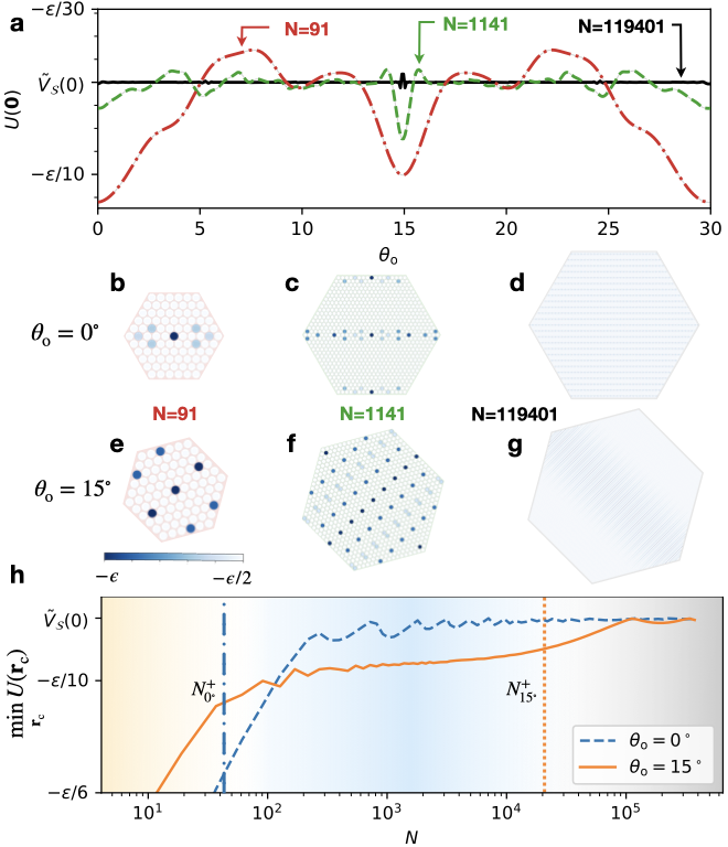
Figure 5: Stability of structural directional lubricity against rotation at finite sizes. (a) The interlocking potential Eq. (2) evaluated at fixed $\mathbf{r}_{\mathrm{c}}=0$ for varying misalignment angle $\theta_{\mathrm{o}}$ for three clusters with size $N=91$, $N=1141$, and $N=119401$, respectively. The contact consists of a triangular-lattice adsorbate spaced by $a=(1+\delta)\sqrt{3/2}$, with $\delta=0.1\%$ on a unit square-lattice substrate. (b–g) Particle-resolved interlocking energy (blue-to-white scale) for the three clusters at two different $\theta_{\mathrm{o}}$, at fixed $\mathbf{r}_{\mathrm{c}}=0$. (h) The minimum value of $U(\mathbf{r}_{\mathrm{c}})$ (minimized by allowing all possible center-mass translations $\mathbf{r}_{\mathrm{c}}$) for fixed alignments $\theta_{\mathrm{o}}=0^{\circ}$ (blue dashed) and $\theta_{\mathrm{o}}=15^{\circ}$ (orange solid), as a function of size $N$. The blue dash-dotted line marks $N_{0^{\circ}}^{+}=40$ and the orange dotted line marks $N_{15^{\circ}}^{+}=17684$.

So far, the relative orientation of the two crystals, has been implicitly fixed by the angle $\theta_{\mathrm{o}}$ between the first primitive vectors of the two lattices, $\mathbf{R}_{1}$ and $\mathbf{S}_{1}$. Clearly, upon rotation the same system may realize a type-A contact (2D array of CLVs), or a type-B contact (1D CLV array), or a type-C contact (fully incommensurate, no CLVs). In practice it is unlikely that one can artificially keep the contact at an arbitrarily fixed mutual angle: in most concrete setups the contact will eventually relax to an energetically stable condition. It is therefore essential to examine the angular energetics of such contacts and their stability upon rotation.

For example, it is well known that structural lubricity in homocontacts arises from the misalignment of the two lattices. However, this misalignment comes with an energy cost, that makes the superlubric contact unstable Dienwiebel et al. (2004); Filippov et al. (2008); de Wijn et al. (2010). In homocontacts therefore energetics acts to stabilize the type-A geometry.

We argue that for heterocontacts the same stabilization occurs. Depending on the geometric details, this stabilization may lead to either a type-A or a type-B contact. Under such conditions, the important outcome is that directional locking and directional structural lubricity are energetically stable. If the crystals mutually rotate from a fully incommensurate kind-C geometry where the interlocking energy is given by Eq. (9), to such an angle that CLVs in the reciprocal space arise, additional terms appear in the interlocking potential of Eqs. (3), leading to potentials of the form (IV.1) or (8). Consequently, for these orientations, these Fourier components in the interlocking potential provide an energy lowering at the equilibrium position, not available in type-C configurations. This means that when a contact allows for type-A or type-B conditions, the corresponding orientations are indeed the most stable ones.

It is straightforward to check this energetics numerically, not only for the infinite contacts of Eq. (3), but also for finite-$N$ cluster of Eq. (14). As an illustration, we select a system quite close to the type-B one of Fig. 1e,f,g,h (triangular-lattice adsorbate over a square substrate), but with a small mismatch $\delta=0.1\%$ introduced in the adsorbate lattice spacing $a=(1+\delta)\sqrt{3/2}$. Due to the small $\delta$, at relative orientation $\theta_{\mathrm{o}}=15^{\circ}$ the CLV $\mathbf{\Omega}$ of Fig. 1f turns into a CMV $\mathbf{G}^{\prime}=2\pi(2,2)$, with a corresponding critical size $N^{+}_{15^{\circ}}\simeq 1.8\times 10^{4}$. To study the relative stability of the consequent nearly-type-B contact, this orientation has to be compared with all others. Figure 5a reports the potential energy $U(\mathbf{r}_{\mathrm{c}}=\mathbf{0})$ of Eq. (2) as a function of the misalignment angle $\theta_{\mathrm{o}}$. The energy profiles of Fig. 5a indicate an evident local energy minimum at $\theta_{\mathrm{o}}=15^{\circ}$ for $N=91$, which becomes the global minimum for $N=1141<N^{+}_{15^{\circ}}$.

For sizes $N\lesssim 100$ the global minimum is found for a different orientation, $\theta_{\mathrm{o}}=0^{\circ}$. This second minimum corresponds to a different (shorter, but worse matched) CMV $\mathbf{G}^{\prime\prime}=2\pi(0,1)$, with critical size $N^{+}_{0^{\circ}}\approx 40$. The moiré patterns associated with these two CMVs at $\theta_{\mathrm{o}}=0^{\circ}$ and $\theta_{\mathrm{o}}=15^{\circ}$ are shown for different sizes in Fig. 5b,c,d and Fig. 5e,f,g, respectively. To illustrate the relative stability between these two orientation, Fig. 5h reports the equilibrium interlocking energy as a function of size. This alternative $\theta_{\mathrm{o}}=0^{\circ}$ orientation is also a nearly-type-B contact. The direct comparison between the CMV at the two orientations of $\tilde{V}_{S}(\mathbf{G}^{\prime})W(\delta\mathbf{\Omega}(\mathbf{G}^{\prime},N))$ and $\tilde{V}_{S}(\mathbf{G}^{\prime\prime})W(\delta\mathbf{\Omega}(\mathbf{G}^{\prime\prime}),N)$ as a function of size gives a crossover point at $N\simeq 100$, which coincides to the crossing point in Fig. 5h, above which $\theta_{\mathrm{o}}=15^{\circ}$ becomes the equilibrium orientation.

At larger sizes, $N\gg N^{+}_{15^{\circ}}$, no CMVs retains a significantly large Fourier component in Eq. (3) and, as expected for a type-C contact, the energy profile as a function of orientation becomes nearly flat, as in the $N=119401$ example of Fig. 5a.

These observations indicate that directional locking and directional structural lubricity are not just a hypothetical eventuality. On the contrary, they prove that with the condition that at some orientation $\theta_{\mathrm{o}}$ the contact geometry generates a CLV, or even just a CMV, sufficiently short to be associated to a sizeable corrugation Fourier component, then precisely this Fourier component is responsible for the energy stabilization of this orientation, which the contact will reach spontaneously if allowed to realign.

Indeed, in the colloidal experimental realizations reported here in Sec. V.4 and in Refs. Cao et al., 2019, 2021 where the clusters are free to reorient, directional locking phenomena and reorientation emerge spontaneously as the result of self-alignment and not of external manipulation.

VII Directional structural lubricity in real-life contacts

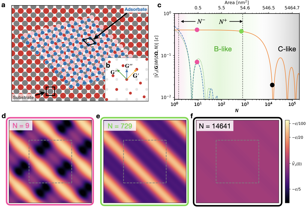
Figure 6: A realistic interface with approximate directional structural lubricity. (a) A monolayer hBN flake (blue dots=B atoms; pink dots=N atoms) deposited on a VO(001) surface (gray dots=V atoms; red dots=O atoms) substrate. The angular misalignment is $\theta_{\mathrm{o}}=15^{\circ}$. (b) Reciprocal lattices of the adsorbate ($\mathcal{Q}$, red) and substrate ($\mathcal{G}$, gray), with marked a CMV $\mathbf{G}^{\prime}$ (orange arrow), a perpendicular reciprocal vector $\mathbf{G}^{\prime\prime}$(green arrow), and the vector $\mathbf{G}^{\prime\prime\prime}$(blue arrow) yielding a sizable Fourier component at small flake size. (c) The size dependence of the Fourier components associated to $\mathbf{G}^{\prime}$ (orange solid line), $\mathbf{G}^{\prime\prime}$ (green dotted), and $\mathbf{G}^{\prime\prime\prime}$ (blue dashed). The vertical lines mark the $\mathbf{G}^{\prime}$ critical sizes $N^{-}\simeq 1$ and $N^{+}=779$ defined in Sect. V.4. (d,e,f) Maps of the interlocking potential $U(\mathbf{r}_{\mathrm{c}})$ in the $[-b,b]\times[-b,b]$ square for the three selected flake sizes marked as matching-colored circles in panel (c); the energy scale is indicated at the right. The dashed gray square delimits the Wigner-Seitz cell of the substrate lattice $\mathcal{S}$.

By taking advantage of CMVs, we can identify interfaces of real materials that should exhibit approximate directional structural lubricity across significant size ranges.

Consider the system depicted in Fig. 6a: for the adsorbate we take a flake of hexagonal boron nitride (hBN), a layered material with hexagonal symmetry and spacing $a=$0.2512\text{\,}\mathrm{n}\mathrm{m}$$ Jain et al. (2013); for the substrate we adopt the (001) surface of VO Della Negra et al. (2000). This surface has square symmetry and spacing $b=$0.310\text{\,}\mathrm{n}\mathrm{m}$$ Jain et al. (2013).

When the hBN flake is rotated at $\theta_{\mathrm{o}}=15^{\circ}$ as in Fig. 6a, the interface exhibits a CMV $\mathbf{G}^{\prime}=2\pi/b(1,1)$ (orange arrow in Fig. 6b), that fosters an energetically stable configuration. The two next most significant Fourier components are associated to $\mathbf{G}^{\prime\prime}=2\pi/b\,(-1,1)$ (perpendicular to $\mathbf{G}^{\prime}$) and $\mathbf{G}^{\prime\prime\prime}=2\pi/b\,(0,1)$.

To illustrate the effect at hand, here we adopt a radically simplified energy landscape, obtained by summing the attraction of each N and B atom in the adsorbate with every substrate atom (regardless of it begin V or O), represented by a negative Gaussian function $V(\mathbf{r})$, with a straightforward extension of Eq. (1). The resulting interlocking potential depends on two parameters only: the width $\sigma=0.1\,b$ of the Gaussian function, and its peak attraction $\epsilon$, which we keep undefined, and adopt as the energy scale of this example, thus expressing all energies in Fig. 6 in terms of $\epsilon$. Of course, a realistic force field would imply quantitatively different Fourier components $V_{\mathcal{S}}(\mathbf{G})$, but we do not expect the results to change radically, because the size-dependent weights $W(\delta\mathbf{\Omega}(\mathbf{G}^{\prime}),N)$ would be identical. Note that $N$ indicates the number of lattice cells, consistently with the rest of the paper. In the hBN flake the total number of atoms is $2N$.

Figure 6c reports the size dependence of the Fourier amplitude $|V_{\mathcal{S}}(\mathbf{G}^{\prime})\,W(\delta\mathbf{\Omega}(\mathbf{G}^{\prime}),N)|$ (solid orange line), plus the analogous quantity for $\mathbf{G}^{\prime\prime}$ (dotted green) and $\mathbf{G}^{\prime\prime\prime}$ (dahsed blue). The $\mathbf{G}^{\prime}$ component dominates across the size range from $N^{-}\simeq 1$ up to a critical size $N^{+}=779$. As a result, at small size, multiple substrate $\mathbf{G}$ vectors contribute significantly to the interlocking potential, resulting in a relatively irregular landscape dominated by pronounced energy corridors modulated by a secondary weaker corrugation, as exemplified in Fig. 6d for $N=9$. This secondary corrugation associated mainly to $\mathbf{G}^{\prime\prime}$ and $\mathbf{G}^{\prime\prime\prime}$ decays rapidly with increasing size, see Fig. 6c. Across the size range $N^{-}\ll N<N^{+}$ spanning over two orders of magnitude in area, the $\pm\mathbf{G}^{\prime}$ Fourier components remain effectively the dominant contribution to the interlocking potential, with the result that this interface exhibits approximate directional structural lubricity as exemplified in Fig. 6e for $N=729$. For sizes larger than $N^{+}$, the energy landscape flattens out and the infinite-size limit of ordinary (kind-C) structural lubricity is approached, as exemplified in Fig. 6f for $N=14641$.

The hBN/VO(001) interface is just an example where we predict directional structural lubricity to arise. Another interface where it could be observed is WSe₂ on CuF(001), as discussed in SI Section 1, and others can be discovered by going through existing materials databases Jain et al. (2013); Mounet et al. (2018); Bergerhoff et al. (1987); Kirklin et al. (2015).

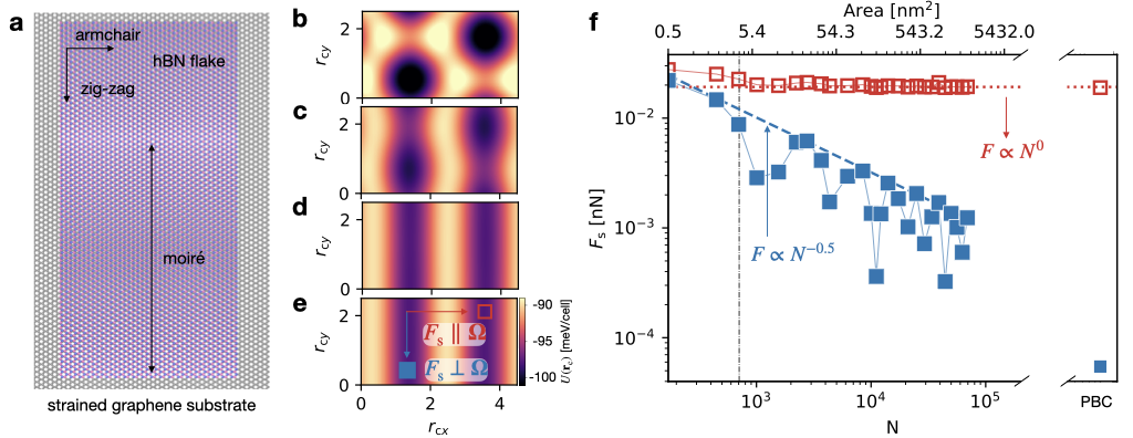
Figure 7: Directional structural lubricity via strain engineering. (a) An aligned hBN flake on a graphene substrate strained by $\varepsilon_{\mathrm{armchair}}\simeq 1.8\%$ in the armchair=$\hat{x}$ direction. The aspect $x:y$ ratio of the hBN flake is approximately $1:2$. The wavelength of the linear moiré pattern is highlighted with a black arrow. (b-e) Corrugation potential $U(\mathbf{r}_{\mathrm{c}})$ for hBN flakes of size (b) 6.5 nm $\times$ 12.7 nm ($N=170$), (c) 13 nm $\times$ 25.5 nm ($N=2760$), (d) 39 nm $\times$ 76.5 nm ($N=11120$), (e) PBC in the region $[0,0.45~{}\text{nm}\times[0,0.25~{}\text{nm}]$. Like in Fig. 6, $N$ is the number of lattice cells, so that the flake consists of $2N$ atoms in total. (f) Static friction in the armchair lattice-matched direction (red empty symbols) and zig-zag (blue filled symbols), respectively parallel and perpendicular to the CLV $\mathbf{\Omega}$. The dashed (dotted) line indicates the scaling in the direction parallel (perpendicular) to the energy corridors, as indicated in panel e. The vertical dash-dotted black line marks the critical size $N_{\mathrm{c}}$ of the largest non-matching component $\mathbf{G}^{\prime}$.

In addition, the geometric conditions for directional structural lubricity can be achieved by means of strain engineering, a method that has been recently used to tailor frictional properties Androulidakis et al. (2020); Zhang et al. (2019); Wang et al. (2019b). For example, the well-studied structurally lubric hBN/graphite contact can be modified by a uni-axial strain applied to the graphite substrate in the armchair direction, as shown in Fig.7a. This deformation, at $\varepsilon_{\mathrm{armchair}}\simeq 1.8\%$, i.e. within experimental feasibility Cao et al. (2020), would generate the geometrical conditions for a type-B directional structural lubricity along the zig-zag direction as discussed in Methods Section XIII. On such a strained graphene surface, we evaluate the static-friction unpinning threshold for aligned hBN flakes of different sizes, based on a realistic force field Brenner et al. (2002); Leven et al. (2016); Kınacı et al. (2012).

Figure 7f reports our prediction for this static-friction force in two orthogonal directions: perpendicular to the valleys of the interlocking potential, i.e. in the strained armchair direction, and parallel to them, i.e. in the unstrained zig-zag direction, as depicted in Fig. 7e. Like in the colloid experiment of Fig. 4, the numerical results agree with the expectation for a type-B contact: in the directions perpendicular to the valleys $F_{\text{s}}\propto N^{0}$, while parallel to the valleys $F_{\text{s}}\propto N^{-1/2}$.

To probe the effect of elasticity, we allow for relaxation of the atomic positions, both of the hBN cluster and of the graphite substrate, while controlling the respective center-of-mass positions. We adopt periodic boundary conditions (PBC), which unavoidably introduce a secondary, much weaker strain on the zig-zag edges. This small strain leads to a commensurate (type-A) configuration, that fits in a periodic cell. This forced commensuration is responsible for the tiny, but nonzero friction in the zig-zag direction reported in the rightmost point in Fig. 7f.

As detailed in the Methods Section XIII, at each center-mass position $\mathbf{r}_{\text{c}}$, we perform a systematic evaluation of the total interlocking energy and lateral force after a full atomic relaxation. The friction force parallel to the valleys after relaxation is nearly a factor three larger than when they are evaluated for rigid layers as reported in Table 2. Despite this reduction, these results indicate that elastic deformations preserve the substantial friction anisotropy.

The adopted value of strain leads to an exact type-B contact. Small deviations from that value would lead to a type-C contact that, for not-too-large hBN clusters, would lead to an approximate type-B behavior, as discussed in Sect. V.4.

VIII Discussion

In this work we formulate a precise classification of the matching/mismatching conditions of 2D crystalline contacts. In addition to the well-known lattice-matching condition and to the structurally lubric fully mismatched condition, we discover an intriguing intermediate condition, characterized by vanishing static friction in just one special direction. We extend this rigorous theory from the rather abstract domain of infinite lattices to the approximate but experimentally more relevant situation of finite-size contacts, where we provide estimations of the range of validity of the resulting frictional regimes.

This theory, summarized in Eqs. (IV.1) and (8), shows how both directional locking and structural lubricity can occur in non-trivial preferential directions, i.e. directions that generally do not coincide with those of highest symmetry for either the substrate or the adsorbate. This is possible only when the dominant contributions to the interlocking potential originates from higher Fourier components $\mathbf{\Omega}$s of the corrugation potential. Non-trivial directions are consequently absent for purely sinusoidal potentials, as was noted in Ref. de Wijn, 2012. Furthermore, the existence of directional structural lubricity is possible only when adsorbate and substrate have either low symmetries or different symmetries (see Methods X). This excludes the commonly studied cases of homocontacts, and even heterocontacts of triangular-on-triangular and square-on-square lattices, which perhaps explains why directional structural lubricity has gone unnoticed so far. Regarding this novel frictional regime, we provide concrete examples of its realization, including an experiment based on colloidal particles driven across a patterned surface.

Most importantly, we investigate the angular energetics of the problem, and show that the same contact orientations that support directional locking and directional structural lubricity are the most energetically stable. Hence the well-known spontaneous decay of superlubricity in homocontacts Filippov et al. (2008) does not apply to directional structural lubricity.

Precisely this intrinsic stability could suggest applications of directional structural lubricity in contexts where a dramatic friction anisotropy is required. The natural field of application involves nanoparticles/nanocontacts, whose small size can accommodate the not-quite-perfect CMVs that one is likely to encounter in real life. By tuning temperature and taking advantage of the different thermal expansion of the contacting materials, or by applying strain to one of the crystals, as discussed in Sec. VII, precise CLVs can be achieved: this condition allows one to realize perfect directional structural lubricity even for a macroscopically large contact, as long as elastic effects are negligible.

The present investigation does not include elasticity. For rigid materials, the effect of the elastic response should remain small and even negligible as long as the contact size remains below a critical value. Such critical sizes range from $N\simeq 10^{5}$ for the colloidal clusters of Fig. 4, to $N\simeq 10^{12}$ corresponding to linear dimensions in the millimeter region for hBN/strained graphene (see Methods XIII) and MoS₂/graphene heterostructures Liao et al. (2022); Cao et al. (2022). For softer materials, or larger sizes, elasticity will acquire an increasingly important role, usually leading to higher friction Sharp et al. (2016); Varini et al. (2015). For type-C contacts, the Aubry-transition paradigm Aubry and Le Daeron (1983); Braun and Kivshar (1998); Brazda et al. (2018) leads us to predict that structural lubricity gives way to a high-friction regime as soon as the strength of the adsorbate-substrate interaction starts to prevail over the adsorbate and substrate rigidity. For soft type-B and near-type-B contacts, we expect a regular 1D Aubry-type physics, although other effects related to Novaco-McTague distortions Novaco and McTague (1977) might play a role too Mandelli et al. (2015, 2017a); Brazda et al. (2018). These questions however go beyond the scope of this paper, and as such their investigation is left to future work.

Author contributions statement

E.P., A.S., and N.M. derived the mathematical formulation. X.C. carried out the experiments. A.S. and E.P. wrote the computer code for the rigid simulations. A.S. and J.W. performed the numerical simulations. All authors contributed to the theoretical understanding, discussed the results and wrote the paper.

Competing Interests

The authors declare no competing interests

Data and Code Availability Statements

Data used in this work is available from the corresponding author on reasonable request.

Materials and Methods

IX Properties of the discrete-coverage dual and real-space lattices

In the discrete-coverage condition, summarized in row A of Table 1, the following two statements hold: (i) for all $\mathbf{Q}_{j}\in\mathcal{Q}$, their components $\mathbf{Q}_{j\mu}/(2\pi)\in\mathbb{Q}$ ($\mu=x,y$), i.e. they are rational numbers; (ii) likewise, for all $\mathbf{R}_{j}\in\mathcal{R}$, their components $\mathbf{R}_{j\mu}\in\mathbb{Q}$, rational numbers too.

The demonstration of (i) goes as follows: we can express any lattice vector in $\mathcal{Q}$ as a linear combination of the primitive lattice vector $\mathbf{Q}_{a}$, $\mathbf{Q}_{b}$, with integer coefficients. In particular, for the lattice vectors $\mathbf{Q}_{1}$, $\mathbf{Q}_{2}$ whose components $\mathbf{Q}_{i\alpha}/(2\pi)$ are integers (line A of Table 1),

$$\mathbf{Q}_{1} =n_{1}\mathbf{Q}_{a}+n_{2}\mathbf{Q}_{b}$$ (1)

$$\mathbf{Q}_{2} =m_{1}\mathbf{Q}_{a}+m_{2}\mathbf{Q}_{b},$$ (2)

with $n_{1},n_{2},m_{1},m_{2}\in\mathbb{Z}$. The relations in Eq. (1), (2) can be inverted to express the primitive vectors in term of $\mathbf{Q}_{1},\mathbf{Q}_{2}$:

$$\mathbf{Q}_{a} =\frac{m_{2}\mathbf{Q}_{1}-n_{2}\mathbf{Q}_{2}}{n_{1}m_{2}-n_{2}m_{1}}$$ (3)

$$\mathbf{Q}_{b} =\frac{-m_{1}\mathbf{Q}_{1}+n_{1}\mathbf{Q}_{2}}{n_{1}m_{2}-n_{2}m_{1}}.$$ (4)

Similar relations hold for these vectors divided by $2\pi$:

$$\frac{\mathbf{Q}_{a}}{2\pi} =\frac{m_{2}\frac{\mathbf{Q}_{1}}{2\pi}-n_{2}\frac{\mathbf{Q}_{2}}{2\pi}}{n_{1}m_{2}-n_{2}m_{1}}$$ (5)

$$\frac{\mathbf{Q}_{b}}{2\pi} =\frac{-m_{1}\frac{\mathbf{Q}_{1}}{2\pi}+n_{1}\frac{\mathbf{Q}_{2}}{2\pi}}{n_{1}m_{2}-n_{2}m_{1}}.$$ (6)

Since at the right hand side of Eqs. (5), (6) all vectors have integer components, the primitive vectors $\mathbf{Q}_{a}/(2\pi),\mathbf{Q}_{b}/(2\pi)$ have rational components. As an arbitrary lattice vector $\mathbf{Q}_{j}\in\mathcal{Q}$ can be written as an integer-coefficient combination of these primitive vectors, $\mathbf{Q}_{j}=l_{1}\mathbf{Q}_{a}+l_{2}\mathbf{Q}_{b}$ (with $l_{1},l_{2}\in\mathbb{Z}$), we conclude that all lattice points in $\mathcal{Q}$ divided by $2\pi$ have rational components.

The demonstration of the real-lattice statement (ii) goes as follows: given the primitive vectors $\mathbf{Q}_{a}$, $\mathbf{Q}_{b}$ of $\mathcal{Q}$, then the primitive vectors of $\mathcal{R}$ can be obtained through the following formulas Ashcroft and Mermin (1976):

$$\mathbf{R}_{a} =2\pi\frac{R_{90}\cdot\mathbf{Q}_{b}}{\mathbf{Q}_{a}\cdot R_{90}\cdot\mathbf{Q}_{b}}=\frac{R_{90}\cdot\frac{\mathbf{Q}_{b}}{2\pi}}{\frac{\mathbf{Q}_{a}}{2\pi}\cdot R_{90}\cdot\frac{\mathbf{Q}_{b}}{2\pi}}$$ (7)

$$\mathbf{R}_{b} =2\pi\frac{R_{90}\cdot\mathbf{Q}_{a}}{\mathbf{Q}_{b}\cdot R_{90}\cdot\mathbf{Q}_{a}}=\frac{R_{90}\cdot\frac{\mathbf{Q}_{a}}{2\pi}}{\frac{\mathbf{Q}_{a}}{2\pi}\cdot R_{90}\cdot\frac{\mathbf{Q}_{b}}{2\pi}}\,,$$ (8)

where $R_{90}$ represents the $2\times 2$ $90^{\circ}$ rotation matrix. The rightmost expressions involve only rational quantities, which proves that $\mathbf{R}_{a}$ and $\mathbf{R}_{b}$ have rational components. As a consequence, all vectors in $\mathcal{R}$ have rational components.

Finally, by multiplying $\mathbf{R}_{a}$ and $\mathbf{R}_{b}$ by the least common denominator of their respective (rational) components, one readily obtains two independent vectors in $\mathcal{R}$ characterized by all integer components.

X Necessary condition for line coverage

To allow for the possibility of line coverage (type B), the two lattices must not share a rotational symmetry of order $n>2$: in practice they cannot be both square or triangular lattices. To prove this, consider two such lattices sharing a rotational symmetry by an angle $\alpha$ of order $n>2$. First of all, if they do not have any nonzero CLV in reciprocal space then they are in the dense coverage case (type C). Let us then assume that they do have a nonzero CLV $\mathbf{\Omega}^{*}$. As a consequence of the common symmetry, also the rotated vector $R_{\alpha}(\mathbf{\Omega}^{*})$ is a CLV (where $R_{\alpha}$ represents a rotation by $\alpha$). Moreover, if the symmetry order is larger than $2$, then $\mathbf{\Omega}^{*}$ and $R_{\alpha}(\mathbf{\Omega}^{*})$ are both CLVs and independent, which leads by definition to the case of discrete coverage, type A. We conclude that to have line coverage (type B) either the two lattices must have different symmetries, or share the same low-order symmetry.

XI Weight function structure factor

When, as is usually the case, $\mathbf{R}^{\text{CLV}}_{1}$ and $\mathbf{R}^{\text{CLV}}_{2}$ are not primitive vectors of $\mathcal{R}$, they define a supercell, namely the unit cell of the moiré pattern formed by $\mathcal{R}$ and $\mathcal{S}$. This supercell contains $K$ vectors $\mathbf{R}^{k}$, such that any lattice-translation vector $\mathbf{R}_{j}$ defining the cluster can now be identified as $\mathbf{R}_{j}=j_{1}\mathbf{R}^{\text{CLV}}_{1}+j_{2}\mathbf{R}^{\text{CLV}}_{2}+\mathbf{R}^{k}$, with $j_{1},j_{2}=-(\sqrt{N^{\prime}}-1)/2,\dots,(\sqrt{N^{\prime}}+1)$, $k=1,\dots,K$, and we assume that $\sqrt{N^{\prime}}$ is an odd integer such that $N=N^{\prime}\,K$.

We then express the weight function as

$$W(\delta\mathbf{\Omega},N)= \frac{1}{N}\!\sum_{j_{1},j_{2},k}\!\!\!\exp(i\delta\mathbf{\Omega}\cdot(j_{1}\mathbf{R}^{\text{CLV}}_{1}+j_{2}\mathbf{R}^{\text{CLV}}_{1}+\mathbf{R}^{k}))$$

$$= \frac{1}{N}\frac{\sin(\sqrt{N^{\prime}}\delta\mathbf{\Omega}\cdot\mathbf{R}^{\text{CLV}}_{1}/2)}{\sin(\delta\mathbf{\Omega}\cdot\mathbf{R}^{\text{CLV}}_{1}/2)}\times$$

$$\quad\frac{\sin(\sqrt{N^{\prime}}\delta\mathbf{\Omega}\cdot\mathbf{R}^{\text{CLV}}_{2}/2)}{\sin(\delta\mathbf{\Omega}\cdot\mathbf{R}^{\text{CLV}}_{2}/2)}\,S(\delta\mathbf{\Omega})\,.$$ (9)

Here we have introduced the supercell "structure factor"

$$S(\delta\mathbf{\Omega})=\sum_{k=1}^{K}\exp(i\delta\mathbf{\Omega}\cdot\mathbf{R}^{k})\,.$$ (10)

The main observation here is that since $\mathbf{R}_{i}^{\mathrm{CLV}}$ are CLV belonging to both $\mathcal{R}$ and $\mathcal{S}$, this structure factor vanishes exactly for all nonzero $\delta\mathbf{\Omega}$’s. By definition $\delta\mathbf{\Omega}\cdot\mathbf{R}_{i}^{\mathrm{CLV}}=\mathbf{G}\cdot\mathbf{R}_{i}^{\mathrm{CLV}}-\mathbf{\bar{Q}}\cdot\mathbf{R}_{i}^{\mathrm{CLV}}=2\pi q$ with $q\in\mathbb{Z}$. Hence, the sinc terms in eq. (9) are equal to $1$ and the weights $W$ associated with any substrate vector $\mathbf{G}$ are size-independent. But only CLV contributions can be size independent and survive for infinite monolayer. Thus the non-CLV contribution must vanish, hence $S(\mathbf{\delta\Omega})=0$.

XII Experimental details

The data shown in Section 4 are obtained using the experimental apparatus described in Cao et al. (2019, 2021), where monolayers of triangularly packed colloidal crystalline clusters of up to hundreds of particles in size are firstly created and then driven across a periodic (square lattice) potential under an applied force. To form the colloidal clusters, we inject a colloidal suspension into a sample cell of $20\times 30\times 0.3~{}\mathrm{mm}^{3}$ in size, where the $0.3~{}\mathrm{mm}$ is the sample thickness and the $20\times 30~{}\mathrm{mm}^{2}$ is the sample area. The colloidal suspension contains a dilute amount ($\sim 10^{7}/\mathrm{mL}$) of colloidal particles (Dynabeads M450 with a diameter of $a=4.45~{}\mu\mathrm{m}$) in a water-based solution that contains a small amount of polyacrylamide (0.02% by weight) and sodium dodecyl sulfate (50% critical micelle concentration). The polyacrylamide induces a bridging flocculation effect which causes the colloidal particles to attract strongly when they get close to each other. Due to gravity, the colloidal particles (buoyant weight $mg=286~{}\mathrm{fN}$) sediment on the bottom surface of the sample cell. Under Brownian motion, the colloidal particles on the sample surface meet one another and aggregate to form random-shaped small clusters up to several tens of particles in size. To facilitate the formation of larger clusters, we tilt the sample so that the small clusters can move quickly on the sample surface and grow larger via accretion. This process also clears the sample surface so that during future sliding the clusters will hardly bump into each other.

The sample surface contains portions of periodically corrugated regions created by photolithography. To create the periodic structures, a thin layer (thickness 100 nm) of photoresist (SU8 2000) was firstly coated to the sample surface and then exposed by UV light (wavelength 365 nm) under a photomask that contains the predefined periodic patterns. The surface is then washed in SU8 developers, after which the unexposed part of the thin film dissolve away, forming a periodically corrugated structure on the surface. This creates a periodic potential for the colloidal particles with a lattice spacing $b=5~{}\mu\mathrm{m}$ and potential barrier $25.8~{}k_{\mathrm{B}}T_{\mathrm{room}}$.

Due to the orientational locking effect, during sliding the clusters will become orientationally locked to an angle $\theta_{\mathrm{o}}=-3.4^{\circ}$ relative to the periodic surface’s lattice direction. At this angle a CMV appears at $\mathbf{G^{\prime}}\approx\mathbf{Q}_{1}-2\mathbf{Q}_{2}$ which leads to a nearly-type-B contact. This creates a low energy corridor along the $25.6^{\circ}$ direction on the interlocking potential energy landscape of the clusters.

To apply a driving force $F$, we tilt the sample in such a way that the in-plane component of the gravitational force is either parallel to the low energy corridor or perpendicular to it. To determine the static friction force component $F_{\mathrm{s}}$ reported in Fig. 4, we firstly increase $F$ in the 80–100 fN region to ensure that the cluster can move along or perpendicular to the low-energy corridor. We then gradually lower $F$ until the cluster is no longer moving: this is the measured $F_{\mathrm{s}}$.

XIII Simulating directional structural lubricity of hBN on strained graphite

We simulate a realistic model for the hBN/strained graphene interaction, consisting of a finite-size rectangular hBN slider in contact with a graphene substrate to which PBC are applied along the armchair ($x$) and zig-zag ($y$) directions, see Fig. 7a. To obtain a contact with a CLV $\mathbf{\Omega}=(4.625,0)~{}\mathrm{nm}^{-1}$ compatible with directional structural lubricity along the zigzag direction , we strain the graphene substrate (with original bond length $1.42039$ Å) along the armchair direction by $\varepsilon_{\mathrm{armchair}}=(a_{\mathrm{hBN}}/b_{\mathrm{graphene}}-1)=1.81799\%$ to match the hBN lattice (bond length $1.44621$ Å), while along the zig-zag direction the graphene substrate is shrunk by $\varepsilon_{\mathrm{zig-zag}}=-0.34542\%$ to account for the Poisson ratio $\nu=0.19$ Jain et al. (2013). The strained graphene has armchair-directed bonds of length 1.44621 Å, zig-zag bonds of length 1.42323 Å, and the angle between them amounts to $120.5357^{\circ}$. The negative stress required for this elongation is estimated to be 8 GPa, assuming a Young modulus of graphene of 1TPa. This is within the experimentally achievable strain of graphene Cao et al. (2020). For all simulations of finite-size hBN clusters, both hBN and graphene are kept rigid. The hBN-graphene interaction is described by the accurate registry-dependent inter-layer potential (ILP) Leven et al. (2014). In this system the reciprocal vector yielding the next most significant Fourier component of the interlocking potential is $\mathbf{G}^{\prime}=(2.312,4.076)~{}\mathrm{nm}^{-1}$.

We also simulate the infinite-size layer, by applying PBC to both hBN and graphene in a common supercell of size $5.64~{}\text{nm}\times 11.5~{}\text{nm}$ ($N=1196$), that imposes a minimal residual strain of 0.00294% to hBN in the zig-zag direction.

Force	Rigid	Flexible
component	[nN]	[nN]
$F_{\mathrm{s}}^{\mathrm{armchair}}$	$1.90\times 10^{-2}$	$2.20\times 10^{-2}$
$F_{\mathrm{s}}^{\mathrm{zig-zag}}$	$5.46\times 10^{-5}$	$1.58\times 10^{-4}$
$F_{\mathrm{s}}^{\mathrm{armchair}}/F_{\mathrm{s}}^{\mathrm{zig-zag}}$	347	140

Table 2: Static friction components for a hBN infinite monolayer (simulated with PBC) dragged along strained graphite. The first column reports the static friction force per cell for a rigid layer (rightmost points in Fig. 7f) and the second column the same quantity evaluated for the flexible case.

The ratio of friction between the pinned armchair direction and the directionally structurally lubric direction is rather large, as expected. Beside simulating rigid layers, in order to probe the effect of elastic deformation, in this PBC model we perform additional flexible simulations, with $z$-direction springs tethered to each slider and substrate atom to mimic the elasticity of the bulk materials Guo et al. (2012). The average external load is kept to zero during the sliding. When modeling the elastic infinite-size contact, both the slider (hBN) and the substrate (graphene) are fully flexible and periodically repeated. The intralayer interaction of hBN and graphene are described by shifted-Tersoff Sevik et al. (2011); Ouyang et al. (2019); Mandelli et al. (2019) and REBO Brenner et al. (2002) force fields, respectively. A standard (quasi-static) simulation protocol Bonelli et al. (2009); Mandelli et al. (2017b) is adopted to compute the interlocking potential energy $U(\mathbf{r}_{\text{c}})$ while changing the position $\mathbf{r}_{\text{c}}$ of the slider relative to the graphene substrate, whose center-of-mass (COM) is kept fixed throughout the simulation. The COM $\mathbf{r}_{\mathrm{c}}$ of the slider is scanned on a $0.1$ Å grid over $x$ and $y$. At fixed COM, the structure is relaxed until the force experienced by each atom decreases below $10^{-5}$ eV/Å. All calculations of the interface potential energy for the rigid layers, and its relaxation in the elastic case are conducted by means of the open-source LAMMPS code Thompson et al. (2022).

After obtaining the energy field $U(\mathbf{r}_{\mathrm{c}})$, we estimate the static friction $F_{\mathrm{s}}$ along the expanded armchair ($\hat{u}_{\mathrm{armchair}}=\hat{x}$) and weakly shrunk zig-zag ($\hat{u}_{\mathrm{zig-zag}}=\hat{y}$) direction by taking the maximum value of $F^{\mathrm{armchair}}=-\hat{u}_{\mathrm{armchair}}\cdot\nabla U$ and $F^{\mathrm{zig-zag}}=-\hat{u}_{\mathrm{zig-zag}}\cdot\nabla U$ between two successive minima, as in Section V.3 and Fig. 3g. Table 2 compares the static friction obtained taking elastic displacement into account with that obtained for the rigid layer.

The overall anisotropy and thus the armchair/zigzag friction ratio, while still very large, is reduced by elasticity. Note that the finite size of the supercell of PBC calculations effectively implements a small-wavevector cutoff, that forbids all long-wavelength deformation. The size at which long-wavelength elastic deformations become important can be estimated by the critical length defined by Sharp et al. Sharp et al. (2016):

$$\lambda=Gd/\tau,$$ (11)

where $G$ is the in-plane shear modulus of the material, $d$ is lattice constant of the substrate, and $\tau$ is the interface shear strength. For the case of hBN on graphite, we obtain a critical length $\lambda=0.662~{}\mathrm{mm}$, using the following values from the literature: $d=0.246~{}\mathrm{nm}$ Brenner et al. (2002), $\tau=0.12~{}\mathrm{MPa}$ Song et al. (2018), $G=2G_{\mathrm{graphene}}G_{\mathrm{hBN}}/(G_{\mathrm{graphene}}+G_{\mathrm{hBN}})$ Johnson and Johnson (1987), with $G_{\mathrm{graphene}}=372~{}\mathrm{GPa}$ and $G_{\mathrm{hBN}}=285~{}\mathrm{GPa}$ Jain et al. (2013).

References

- Mo et al. (2009) Y. Mo, K. T. Turner, and I. Szlufarska, Nature 457, 1116 (2009).
- Guerra et al. (2010) R. Guerra, U. Tartaglino, A. Vanossi, and E. Tosatti, Nature Materials 9, 634 (2010).
- Kawai et al. (2016) S. Kawai, A. Benassi, E. Gnecco, H. Söde, R. Pawlak, X. Feng, K. Müllen, D. Passerone, C. A. Pignedoli, P. Ruffieux, R. Fasel, and E. Meyer, Science 351, 957 (2016).
- Liu et al. (2020) B. Liu, J. Wang, S. Zhao, C. Qu, Y. Liu, L. Ma, Z. Zhang, K. Liu, Q. Zheng, and M. Ma, Science Advances 6, eaaz6787 (2020).
- He et al. (1999) G. He, M. H. Muser, and M. O. Robbins, Science 284, 1650 (1999).
- Hirano et al. (1997) M. Hirano, K. Shinjo, R. Kaneko, and Y. Murata, Physical Review Letters 78, 1448 (1997).
- Feng et al. (2013) X. Feng, S. Kwon, J. Y. Park, and M. Salmeron, ACS Nano 7, 1718 (2013).
- Dietzel et al. (2008) D. Dietzel, C. Ritter, T. Mönninghoff, H. Fuchs, A. Schirmeisen, and U. D. Schwarz, Physical Review Letters 101, 125505 (2008).
- Gigli et al. (2018) L. Gigli, N. Manini, E. Tosatti, R. Guerra, and A. Vanossi, Nanoscale 10, 2073 (2018).
- Silva et al. (2022) A. Silva, E. Tosatti, and A. Vanossi, Nanoscale 14, 6384 (2022).
- Novoselov et al. (2016) K. Novoselov, o. A. Mishchenko, o. A. Carvalho, and A. Castro Neto, Science 353, aac9439 (2016).
- Hod et al. (2018) O. Hod, E. Meyer, Q. Zheng, and M. Urbakh, Nature 563, 485 (2018).
- Vanossi et al. (2020) A. Vanossi, C. Bechinger, and M. Urbakh, Nature Communications 11, 4657 (2020).
- Song et al. (2018) Y. Song, D. Mandelli, O. Hod, M. Urbakh, M. Ma, and Q. Zheng, Nature Materials 17, 894 (2018).
- Baykara et al. (2018) M. Z. Baykara, M. R. Vazirisereshk, and A. Martini, Applied Physics Reviews 5, 041102 (2018).
- Cao et al. (2019) X. Cao, E. Panizon, A. Vanossi, N. Manini, and C. Bechinger, Nature Physics 15, 776 (2019).
- Cao et al. (2021) X. Cao, E. Panizon, A. Vanossi, N. Manini, E. Tosatti, and C. Bechinger, Physical Review E 103, 1 (2021).
- de Wijn (2012) A. S. de Wijn, Physical Review B 86, 85429 (2012).
- Dietzel et al. (2013) D. Dietzel, M. Feldmann, U. D. Schwarz, H. Fuchs, and A. Schirmeisen, Physical Review Letters 111, 235502 (2013).
- Hod (2013) O. Hod, ChemPhysChem 14, 2376 (2013).
- Braun and Kivshar (1998) O. M. Braun and Y. S. Kivshar, Physics Reports 306, 1 (1998).
- Benassi et al. (2015) A. Benassi, M. Ma, M. Urbakh, and A. Vanossi, Scientific reports 5, 1 (2015).
- Sharp et al. (2016) T. A. Sharp, L. Pastewka, and M. O. Robbins, Physical Review B 93, 121402 (2016).
- Gnecco et al. (2001) E. Gnecco, R. Bennewitz, T. Gyalog, and E. Meyer, Journal of Physics: Condensed Matter 13, R619 (2001).
- Fusco and Fasolino (2005) C. Fusco and A. Fasolino, Physical Review B 71, 45413 (2005).
- Brazda et al. (2018) T. Brazda, A. Silva, N. Manini, A. Vanossi, R. Guerra, E. Tosatti, and C. Bechinger, Physical Review X 8, 011050 (2018).
- Norell et al. (2016) J. Norell, A. Fasolino, and A. S. de Wijn, Physical Review E 94, 023001 (2016).
- Micciancio and Goldwasser (2002) D. Micciancio and S. Goldwasser, Complexity of lattice problems: a cryptographic perspective, Vol. 671 (Springer Science & Business Media, 2002).
- Micciancio (2010) D. Micciancio, “Cse 206a: Lattice algorithms and applications,” (2010).
- Frenkel and Kontorova (1938) Y. I. Frenkel and T. Kontorova, Physikalische Zeitschrift der Sowjetunion 13, 1 (1938).
- Aubry and Le Daeron (1983) S. Aubry and P.-Y. Le Daeron, Physica D: Nonlinear Phenomena 8, 381 (1983).
- Braun and Kivshar (2004) O. M. Braun and Y. S. Kivshar, The Frenkel-Kontorova model: concepts, methods, and applications (Springer, 2004).
- Note (1) A set is dense if it has the following property: for any and for any point in the vector space, there exists a such that .
- Bohlein and Bechinger (2012) T. Bohlein and C. Bechinger, Physical Review Letters 109, 058301 (2012).
- Korda et al. (2002) P. T. Korda, M. B. Taylor, and D. G. Grier, Physical Review Letters 89, 128301 (2002).
- Trillitzsch et al. (2018) F. Trillitzsch, R. Guerra, A. Janas, N. Manini, F. Krok, and E. Gnecco, Physical Review B 98, 1 (2018).
- Villegas et al. (2003) J. Villegas, E. Gonzalez, M. Montero, I. K. Schuller, and J. Vicent, Physical Review B 68, 224504 (2003).
- Reichhardt and Nori (1999) C. Reichhardt and F. Nori, Physical Review Letters 82, 414 (1999).
- Gopinathan and Grier (2004) A. Gopinathan and D. G. Grier, Physical Review Letters 92, 130602 (2004).
- Frechette and Drazer (2009) J. Frechette and G. Drazer, Journal of fluid mechanics 627, 379 (2009).
- Speer et al. (2010) D. Speer, R. Eichhorn, and P. Reimann, Physical Review Letters 105, 090602 (2010).
- Reichhardt and Reichhardt (2011) C. Reichhardt and C. O. Reichhardt, Physical Review Letters 106, 060603 (2011).
- Pelton et al. (2004) M. Pelton, K. Ladavac, and D. G. Grier, Physical Review E 70, 031108 (2004).
- Dienwiebel et al. (2004) M. Dienwiebel, G. S. Verhoeven, N. Pradeep, J. W. M. Frenken, J. A. Heimberg, and H. W. Zandbergen, Physical Review Letters 92, 126101 (2004).
- Born and Wolf (2013) M. Born and E. Wolf, Principles of optics: electromagnetic theory of propagation, interference and diffraction of light (Elsevier, 2013).
- Ashcroft and Mermin (1976) N. W. Ashcroft and N. D. Mermin, Solid State Physics (Holt, Rinehart and Winston,, 1976).
- Koren and Duerig (2016) E. Koren and U. Duerig, Physical Review B 94, 1 (2016).
- Wang et al. (2019a) J. Wang, W. Cao, Y. Song, C. Qu, Q. Zheng, and M. Ma, Nano Letters 19, 7735 (2019a).
- Cao et al. (2022) X. Cao, A. Silva, E. Panizon, A. Vanossi, N. Manini, E. Tosatti, and C. Bechinger, Phys. Rev. X 12, 021059 (2022).
- Filippov et al. (2008) A. E. Filippov, M. Dienwiebel, J. W. M. Frenken, J. Klafter, and M. Urbakh, Physical Review Letters 100, 046102 (2008).
- de Wijn et al. (2010) A. S. de Wijn, C. Fusco, and A. Fasolino, Physical Review E 81, 046105 (2010).
- Jain et al. (2013) A. Jain, S. P. Ong, G. Hautier, W. Chen, W. D. Richards, S. Dacek, S. Cholia, D. Gunter, D. Skinner, G. Ceder, et al., APL materials 1, 011002 (2013).
- Della Negra et al. (2000) M. Della Negra, M. Sambi, and G. Granozzi, Surface Science 461, 118 (2000).
- Mounet et al. (2018) N. Mounet, M. Gibertini, P. Schwaller, D. Campi, A. Merkys, A. Marrazzo, T. Sohier, I. E. Castelli, A. Cepellotti, G. Pizzi, and N. Marzari, Nature Nanotechnology 13, 246 (2018).
- Bergerhoff et al. (1987) G. Bergerhoff, I. D. Brown, F. Allen, et al., International Union of Crystallography, Chester 360, 77 (1987).
- Kirklin et al. (2015) S. Kirklin, J. E. Saal, B. Meredig, A. Thompson, J. W. Doak, M. Aykol, S. Rühl, and C. Wolverton, npj Computational Materials 1, 1 (2015).
- Androulidakis et al. (2020) C. Androulidakis, E. N. Koukaras, G. Paterakis, G. Trakakis, and C. Galiotis, Nature Communications 11 (2020), 10.1038/s41467-020-15446-y.
- Zhang et al. (2019) S. Zhang, Y. Hou, S. Li, L. Liu, Z. Zhang, X.-Q. Feng, and Q. Li, Proceedings of the National Academy of Sciences 116, 24452 (2019).
- Wang et al. (2019b) K. Wang, W. Ouyang, W. Cao, M. Ma, and Q. Zheng, Nanoscale 11, 2186 (2019b).
- Cao et al. (2020) K. Cao, S. Feng, Y. Han, L. Gao, T. Hue Ly, Z. Xu, and Y. Lu, Nature communications 11, 1 (2020).
- Brenner et al. (2002) D. W. Brenner, O. A. Shenderova, J. A. Harrison, S. J. Stuart, B. Ni, and S. B. Sinnott, Journal of Physics-Condensed Matter 14, 783 (2002).
- Leven et al. (2016) I. Leven, T. Maaravi, I. Azuri, L. Kronik, and O. Hod, Journal of Chemical Theory and Computation 12, 2896 (2016).
- Kınacı et al. (2012) A. Kınacı, J. B. Haskins, C. Sevik, and T. Çağın, Physical Review B 86, 115410 (2012).
- Liao et al. (2022) M. Liao, P. Nicolini, L. Du, J. Yuan, S. Wang, H. Yu, J. Tang, P. Cheng, K. Watanabe, T. Taniguchi, et al., Nature Materials 21, 47 (2022).
- Varini et al. (2015) N. Varini, A. Vanossi, R. Guerra, D. Mandelli, R. Capozza, and E. Tosatti, Nanoscale 7, 2093 (2015).
- Novaco and McTague (1977) A. D. Novaco and J. P. McTague, Physical Review Letters 38, 1286 (1977).
- Mandelli et al. (2015) D. Mandelli, A. Vanossi, N. Manini, and E. Tosatti, Physical Review Letters 114, 108302 (2015).
- Mandelli et al. (2017a) D. Mandelli, A. Vanossi, N. Manini, and E. Tosatti, Physical Review B 95, 245403 (2017a).
- Leven et al. (2014) I. Leven, I. Azuri, L. Kronik, and O. Hod, The Journal of Chemical Physics 140, 104106 (2014).
- Guo et al. (2012) Z. Guo, T. Chang, X. Guo, and H. Gao, Journal of the Mechanics and Physics of Solids 60, 1676 (2012).
- Sevik et al. (2011) C. Sevik, A. Kinaci, J. B. Haskins, and T. Çağın, Physical Review B 84, 085409 (2011).
- Ouyang et al. (2019) W. Ouyang, I. Azuri, D. Mandelli, A. Tkatchenko, L. Kronik, M. Urbakh, and O. Hod, Journal of Chemical Theory and Computation 16, 666 (2019).
- Mandelli et al. (2019) D. Mandelli, W. Ouyang, M. Urbakh, and O. Hod, ACS Nano 13, 7603 (2019).
- Bonelli et al. (2009) F. Bonelli, N. Manini, E. Cadelano, and L. Colombo, The European Physical Journal B 70, 449 (2009).
- Mandelli et al. (2017b) D. Mandelli, I. Leven, O. Hod, and M. Urbakh, Scientific Reports 7, 1 (2017b).
- Thompson et al. (2022) A. P. Thompson, H. M. Aktulga, R. Berger, D. S. Bolintineanu, W. M. Brown, P. S. Crozier, P. J. in ’t Veld, A. Kohlmeyer, S. G. Moore, T. D. Nguyen, R. Shan, M. J. Stevens, J. Tranchida, C. Trott, and S. J. Plimpton, Computer Physics Communications 271 (2022), 10.1016/j.cpc.2021.108171.
- Johnson and Johnson (1987) K. L. Johnson and K. L. Johnson, Contact mechanics (Cambridge university press, 1987).