RepGhost: A Hardware-Efficient Ghost Module via Re-parameterization

Abstract

Feature reuse has been a key technique in light-weight convolutional neural networks (CNNs) design. Current methods usually utilize a concatenation operator to keep large channel numbers cheaply (thus large network capacity) by reusing feature maps from other layers. Although concatenation is parameters- and FLOPs-free, its computational cost on hardware devices is non-negligible. To address this, this paper provides a new perspective to realize feature reuse via structural re-parameterization technique. A novel hardware-efficient RepGhost module is proposed for implicit feature reuse via re-parameterization, instead of using concatenation operator. Based on the RepGhost module, we develop our efficient RepGhost bottleneck and RepGhostNet. Experiments on ImageNet and COCO benchmarks demonstrate that the proposed RepGhostNet is much more effective and efficient than GhostNet and MobileNetV3 on mobile devices. Specially, our RepGhostNet surpasses GhostNet 0.5$\times$ by 2.5% Top-1 accuracy on ImageNet dataset with less parameters and comparable latency on an ARM-based mobile phone. Code is available at https://github.com/ChengpengChen/RepGhost.

1 Introduction

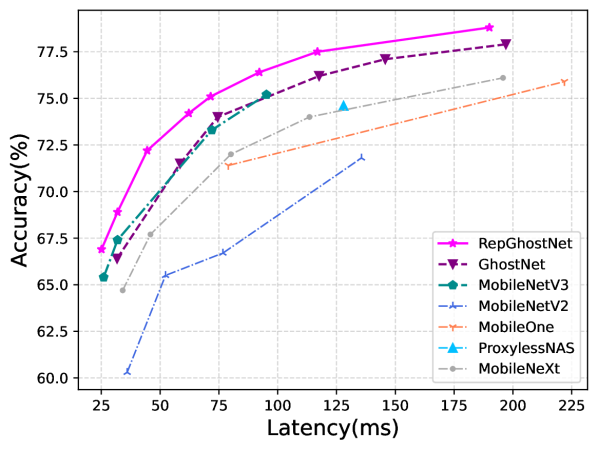
Figure 1: Top-1 accuracy on ImageNet vs. latency on an ARM-based mobile phone, refer to Sec. 4 for the detail.

With the mobile and portable devices being ubiquitous, efficient convolutional neural networks (CNNs) are becoming indispensable due to the limited computational resources. Different methods are proposed to achieve the same goal of making CNNs more efficient in recent years, such as light-weight architecture design[31, 20, 35, 14, 48, 3], neural architecture search[38, 27, 13, 44], pruning[30, 32, 2, 18], etc, and much progress has been made.

In the field of architecture design, large number of channels often means large network capacity[17, 24, 23], especially for light-weight CNNs[31, 35, 19, 14]. As stated in [31], given a fixed FLOPs, the light-weight CNNs prefer to use spare connections (e.g. , group or depthwise convolution) and feature reuse. They both have been well-explored and many representative light-weight CNNs have been proposed in recent years[20, 35, 19, 47, 31, 48, 5, 14, 15]. Spare connections are designed to keep large network capacity with low floating-point operations (FLOPs), while feature reuse aims to explicitly keep large number of channel (thus large network capacity) by simply concatenating existing feature maps from different layers[24, 23, 14, 37]. For example, in DenseNet[24], feature maps of previous layers are reused and sent to their subsequent layers within a stage, resulting in more and more channels. GhostNet[14, 15] proposes to generate more feature maps from cheap operations, and concatenate them with original ones for keeping large number of channels. ShuffleNetV2[31] processes only half of channels and keep the other half to be concatenated. They all utilize feature reuse via concatenation operation to enlarge channel numbers and network capacity while keeping FLOPs low. It seems that concatenation has been a standard and elegant operation for feature reuse.

Concatenation is parameters- and FLOPs-free, however, its computational cost on hardware devices is non-negligible, since parameters and FLOPs are not direct cost indicators for actual runtime performance of machine learning models[8, 31]. To verify this, we provide detailed analysis in Sec. 3.1. We found that concatenation operation is much more inefficient than add operation on hardware devices due to its complicated memory copy. Therefore, it is noteworthy to explore a better and more hardware-efficient way for feature reuse beyond concatenation operation.

Recently, structural re-parameterization has proved its effectiveness in CNNs architecture design, including DiracNet[46], ExpandNets[12], ACNet[10], RepVGG[11], etc. It can convert the complex training-time architecture into a simpler inference-time one equivalently in the weight space without any time-cost. Inspired by this, we propose to utilize structural re-parameterization, instead of the widely-used concatenation, to realize feature reuse implicitly for hardware-efficient architecture design.

In this paper, we propose a hardware-efficient RepGhost module via structural re-parameterization to realize feature reuse implicitly. Note that it is not just to apply re-parameterization technique to existing layer in Ghost module, but to improve the module for faster inference. To be specific, we first remove the inefficient concatenation operator, and then modify the architecture to satisfy the rule of structural re-parameterization. Therefore, the feature reuse process can be moved from feature space to weight space before inference, making our module efficient. Finally, based on RepGhost module, we develop a hardware-efficient CNNs denoted as RepGhostNet, which outperforms previous state-of-the-art light-weight CNNs in accuracy-latency trade-off, as shown in Fig. 1. Our contributions are summarized as follows.

• We show that concatenation operation is not cost-free and indispensable for feature reuse in hardware-efficient architecture design, and propose a new perspective to realize feature reuse via structural re-parameterization technique.

• We propose a novel RepGhost module with implicit feature reuse and develop a more hardware-efficient RepGhostNet compared to GhostNet[14] and MobileNetV3[19].

• We show that our RepGhostNet can achieve better performance on several vision tasks, compared to previous state-of-the-art light-weight CNNs with lower mobile latency.

2 Related Work

2.1 Light-weight CNNs

Both manual designed[20, 47, 35, 48, 3] and neural architecture search (NAS)[44, 42, 7, 13, 22] based light-weight CNNs are mainly designed to get competitive performances with less parameters and low FLOPs. Among them, ShuffleNetV1[47] and MobileNetV2[35] establish the benchmark by using massive depthwise convolutions rather than the dense ones. FBNet[44, 42] employ complex NAS technique to design light-weight architecture automatically. However, parameters and FLOPs often can not reflect the actual runtime performance ($i.e.$, latency) of light-weight CNNs[31, 8]. And few models are designed for low latency directly, like ProxylessNAS[27], MNASNet[38], MobileNetV3[19], and ShuffleNetV2[31]. This paper follows this to design efficient CNNs with low latency.

On the other hand, feature reuse in CNNs has also inspired many impressive works[24, 45, 23, 14, 15, 31, 37] with cheap or even free costs. As light-weight CNNs, GhostNet[14] uses cheap operations to produce more channels with low computational costs, and ShuffleNetV2[31] processes only half of channels of features and keep the other half to be concatenated. They all use concatenation operation to keep large channel numbers since it is parameters- and FLOPs-free. But we note that it is inefficient on mobile devices due to its complicated memory copy process, making it not indispensable for feature reuse in light-weight CNNs. Therefore, in this paper, we explore to utilize feature reuse in light-weight CNNs architecture design beyond concatenation operation.

2.2 Structural Re-parameterization

Structural re-parameterization is generally to transform the more expressive and complex architecture at training time into a simpler one for fast inference. ExpandNets[12] re-parameterizes the linear layers in the model into several continuous linear layers during training. ACNet[10] and RepVGG[11] decompose a single convolutional layer into a training-time multi-branch block. For example, one such training-time block in RepVGG contains three parallel layers, $i.e.$, 3x3 convolution, 1x1 convolution and identity mapping, and an add operator to fuse their output features. During inference, the fusion process can be moved from feature space to weight space, resulting in a simple block for inference (only one 3x3 convolution)[11]. This motivates us to design light-weight CNNs with efficient inference architectures using this technique.

Recently, structural re-parameterization technique is also employed in MobileOne[41] to remove shortcut (or skip connection) and design mobile backbone for the powerful NPU in iPhone12 with large FLOPs. In this paper, however, we note that shortcut is necessary and will not bring much time-cost in extremely light-weight CNNs (See Sec. 4.3). We utilize re-parameterization technique to realize feature reuse implicitly by replacing the inefficient concatenation operator in Ghost module, which makes our RepGhostNet more efficient on computation-constrained mobile devices.

3 Method

In this section, we will first revisit concatenation operation for feature reuse, and introduce how to utilize structural re-parameterization to achieve this. Based on it, we propose a novel re-parameterized module for implicit feature reuse, $i.e.$, RepGhost module. After that, we describe our hardware-efficient network built on this module, which is denoted as RepGhostNet.

3.1 Feature Reuse via Re-parameterization

Feature reuse has been widely used in CNNs to enlarge the network capacity, such as DenseNet[24], ShuffleNetV2[31] and GhostNet[14]. Most methods utilize the concatenation operator combining feature maps from different layers to produce more features cheaply. Concatenation is parameters- and FLOPs-free, however, its computational cost is non-negligible due to the complicated memory copy on hardware devices. To address this, we provide a new perspective to realize feature reuse implicitly: feature reuse via structural re-parameterization.

Concatenation costs. As mentioned above, memory copy in concatenation brings non-negligible computational costs on hardware devices. For example, let $M_{1}\in\mathbb{R}^{N\times C_{1}\times H\times W}$ and $M_{2}\in\mathbb{R}^{N\times C_{2}\times H\times W}$ be two feature maps in data layout NCHW to be concatenated alone channel dimension. The largest contiguous blocks of memory required when processing $M_{1}$ and $M_{2}$ are $b_{1}\in\mathbb{R}^{1\times C_{1}\times H\times W}$ and $b_{2}\in\mathbb{R}^{1\times C_{2}\times H\times W}$, respectively. Concatenating $b_{1}$ and $b_{2}$ is direct, and this process would repeat $N$ times. For data in layout NHWC[1], the largest contiguous block of memory is much smaller, i.e., $b_{1}\in\mathbb{R}^{1\times 1\times 1\times{C_{1}}}$, making the copy process more complicated. While for element-wise operators, like Add, the largest contiguous blocks of memory are $M_{1}$ and $M_{2}$ themselves, making the operations much easier.

Operator	Latency(ms)
	bs=1	2	8	32
Concatenation	5.2	13.2	64.24	292.2
Add	2.6	6.7	34.0	149.8

Table 1: Runtime of concatenation and add operators with different batch sizes on an ARM-based mobile phone.

To evaluate the concatenation operation quantitatively, we analyze its actual runtime on a mobile device. We take GhostNet 1.0x[14] as an example, and replace all its concatenation operators with add operators for comparison, which is also a simple operator to process different features with low costs[17, 36]. Note that these two operators operate on tensors with exactly the same shape. Table. 1 shows the accumulated runtime of all 32 corresponding operators in the corresponding network. Concatenation costs $\sim$2x times over Add. We also plot the time percentages under different batch sizes in Fig. 2. With batch size increases, the gap of runtime percentage between concatenation and add becomes larger, which is consistent with our data layout analysis.

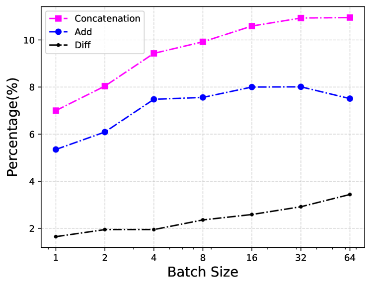
Figure 2: Runtime percentage of each operator in the entire network. Diff: the percent difference between concatenation and add.

Re-parameterization vs. Concatenation Let $y\in\mathbb{R}^{N\times C_{out}\times H\times W}$ denotes the output with $C_{out}$ channels and $x\in\mathbb{R}^{N\times C_{in}\times H\times W}$ denotes the input to be processed and reused. $\Phi_{i}(x),\forall i=1,\ldots,s-1$ denote other neural network layers, such as convolution or BN, applied to x. Without loss of generality, feature reuse via concatenation can be expressed as:

$$y=Cat([x,\Phi_{1}(x),\ldots,\Phi_{s-1}(x)])$$ (1)

where $Cat$ is the concatenation operation. It simply keeps existing feature maps and leaves the information processing to other operators. For example, a concatenation layer is usually followed by an 1$\times$1 dense convolutional layer to process the channel information[37, 24, 14]. However, as Table. 1 shows, concatenation is not cost-free for feature reuse on hardware devices, which motivates us to find a more efficient way.

Recently, structural re-parameterization has been treated as a cost-free technique to improve the performance of CNNs in many works[10, 11, 41]. Inspired by this, we note that structural re-parameterization can also be treated as an efficient technique for implicit feature reuse, so as to design more hardware-efficient CNNs. For example, structural re-parameterization usually utilizes several linear operators to produce diverse feature maps during training, and fuse all operators into one via parameters fusion for fast inference. That is, it moves the fusion process from feature space to weight space, which can be treated as an implicit way for feature reuse. Follow the symbols in Eq.1, feature reuse via structural re-parameterization can be expressed as:

$$y=Add([x,\Phi_{1}(x),\ldots,\Phi_{s-1}(x)])=\Phi^{\ast}(x)$$ (2)

Different from concatenation, add also plays a feature fusion role. All operation $\Phi_{i}(x),\forall i=1,\ldots,s-1$ in structural re-parameterization are linear function, and will be fused into $\Phi^{\ast}(x)$ finally. The feature fusion process is done in the weight space, which will not introduce any extra inference time, making the final architecture more efficient than that with concatenation. As shown in Fig. 2, implementing feature reuse via structural re-parameterization can save $7\%\sim 11\%$ time compared to concatenation and $5\%\sim 8\%$ to add. Based on this concept, we propose a hardware-efficient RepGhost module with feature reuse via structural re-parameterization in the following subsection.

3.2 RepGhost Module

To make use of feature reuse via re-parameterization, this subsection introduces how Ghost module evolves to our RepGhost module. It is non-trivial to apply re-parameterization to original Ghost module directly due to concatenation operator. Several adjustments are made to derive our RepGhost module. As Fig. 3 shows, we start from Ghost module in Fig. 3a and adjust the intra components progressively.

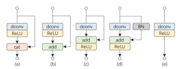
Figure 3: Evolution from Ghost module to our RepGhost module. We omit the input 1x1 convolution for simplicity, refer to Fig. 4 for more structure details. dconv: depthwise convolutional layer (followed by a BN). cat: concatenation layer. a) Ghost module[14] with ReLU; b) replacing concatenation with add; c) moving ReLU backward to make the module satisfying the rule of structural re-parameterization; d) RepGhost module during training; e) RepGhost module during inference. Module $c$ and $d$ can be fused into module $e$ during inference.

Add Operator. Due to the inefficiency of concatenation for feature reuse discussed in Sec. 3.1, we first replace concatenation operator with add operator[17, 36] to get module $b$ in Fig. 3b. It should provide higher efficiency as shown in Table. 1 and Fig. 2.

Moving ReLU Backward. In the spirit of structural re-parameterization[10, 11], we move the ReLU after depthwise convolutional layer backward, $i.e.$, after add operator, as module $c$ shown in Fig. 3c. This movement makes the module satisfying the rule of structural re-parameterization[11, 10], and thus available to be fused into module $e$ for fast inference. The effect of moving ReLU backward will be discussed in Sec. 4.3.

Re-parameterization. As a re-parameterized module, module $c$ can be more flexible in the re-parameterization structure rather than identity mapping[10, 41]. As module $d$ shown in Fig. 3d, we simply add Batch Normalization(BN)[25] in the identity branch, which brings non-linearity during training and can be fused for fast inference. This module is denoted as our RepGhost module. We also explore other re-parameterization structures in Sec. 4.3.

Fast Inference. As re-parameterized modules, module $c$ and module $d$ can be fused into module $e$ in Fig. 3e for fast inference. Our RepGhost module has a simple inference structure which only contains regular convolution layers and ReLU, making it hardware-efficient[11]. Specifically, the feature fusion process is carried out in weight space rather than feature space, $i.e.$, fusing parameter of each branch and producing a simplified structure for fast inference, which makes it cost-free. Due to the linearity of each operator, the parameter fusion process is direct (see [10, 11] for the detail).

Comparison with Ghost module. GhostNet[14] proposes to generate more feature maps from cheap operations, so it can enlarge the network capacity in a low-cost way. In our RepGhost module, we further propose a more efficient way to generate and fuse diverse feature maps via re-paramterization. Different from Ghost module, RepGhost module removes the inefficient concatenation operator, saving much inference time. And the information fusion process is executed by add operator in an implicit way, instead of leaving to other convolutional layers.

In GhostNet[14], Ghost module has a ratio $s$ to control the complexity. According to Eq. 1, $C_{in}=\frac{1}{s}*C_{out}$ and the rest $\frac{s-1}{s}*C_{out}$ channels are produced by depthwise convolutions $\Phi_{i},\forall i=1,\ldots,s-1$. While the final outputs $C_{out}$ of our RepGhost are equal to $C_{in}$. RepGhost module produce $s*C_{in}$ channels during the training, and fuse them into $C_{in}$ channels for inference, which not only keeps the generation of diverse feature maps, but also saves the inference time on hardware devices.

3.3 Building our Bottleneck and Architecture

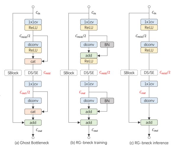
Figure 4: RepGhost bottleneck compared to Ghost bottleneck[14]. SBlock: shortcut block, DS: downsample layer, SE: SE block[21]. RG-bneck: RepGhost bottleneck. The blocks in dash line are only inserted if necessary. $C_{in},C_{mid}$ and $C_{out}$ denote input, middle and output channels of the bottlenecks, respectively. Note that RepGhost bottleneck differs to Ghost bottleneck in channels inside the bottlenecks, which are masked as red.

RepGhost Bottleneck. Based on Ghost bottleneck[14] in Fig. 4a, we replace the Ghost modules with RepGhost modules directly to build our RepGhost bottleneck. However, the add operator in RepGhost module differs to the concatenation operator in Ghost module in output channels, e.g. , 50% of the latter. Simply changing the input channel of the following layer will change the network severely. To address this, RepGhost bottleneck keeps the input and output channel numbers same as Ghost bottleneck. As Fig. 4b shows, RepGhost bottleneck has two changes in channel setting compared to Ghost bottleneck: a) ”thinner” middle channels, and b) ”thicker” channels for second depthwise convolutional layer. Firstly, applying downsample and SE on feature maps with decreased channels makes RepGhost bottleneck more efficient[34]. Secondly, applying depthwise convolution on feature maps with increased channels enlarges the network capacity[35], thus making RepGhost bottleneck more effective. Due to structural re-parameterization, RepGhost bottleneck only contains 2 branches (Fig. 4c) during inference: a shortcut and a single chain of operators (1$\times$1 convolution, depthwise convolution and ReLU), making it more efficient in memory cost and fast inference[31, 11]. We will discuss the necessity of shortcut in Sec. 4.3 and profile the actual runtime on mobile devices to demonstrate the hardware efficiency over Ghost bottleneck.

Input	Operator	$\#$mid	$\#$out	SE	Stride
$224^{2}\times 3$	Conv$3\times 3$	-	16	-	2
$112^{2}\times 16$	RG-bneck	8	16	-	1
$112^{2}\times 16$	RG-bneck	24	24	-	2
$56^{2}\times 24$	RG-bneck	36	24	-	1
$56^{2}\times 24$	RG-bneck	36	40	1	2
$28^{2}\times 40$	RG-bneck	60	40	1	1
$28^{2}\times 40$	RG-bneck	120	80	-	2
$14^{2}\times 80$	RG-bneck	100	80	-	1
$14^{2}\times 80$	RG-bneck	120	80	-	1
$14^{2}\times 80$	RG-bneck	120	80	-	1
$14^{2}\times 80$	RG-bneck	240	112	1	1
$14^{2}\times 112$	RG-bneck	336	112	1	1
$14^{2}\times 112$	RG-bneck	336	160	1	2
$7^{2}\times 160$	RG-bneck	480	160	-	1
$7^{2}\times 160$	RG-bneck	480	160	1	1
$7^{2}\times 160$	RG-bneck	480	160	-	1
$7^{2}\times 160$	RG-bneck	480	160	1	1
$7^{2}\times 160$	Conv$1\times 1$	-	960	-	1
$7^{2}\times 960$	AvgPool	-	960	-	-
$1^{2}\times 960$	Conv$1\times 1$	-	1280	-	1
$1^{2}\times 1280$	Conv$1\times 1$	-	1000	-	1

Table 2: Overall architecture of RepGhostNet. $\#$mid means middle channel inside the bottleneck. Note that it correspondences to $C_{mid}/2$ in Fig. 4. $\#$out means the number of output channels. SE denotes whether using SE block.

RepGhostNet. With the RepGhost bottleneck built above and its input and output channel numbers same as Ghost bottleneck, RepGhostNet can be simply built by replacing Ghost bottleneck in GhostNet [14] with our RepGhost bottleneck. The architecture detail is shown in Table. 2. RepGhostNet stacks RepGhost bottlenecks except the input and output layers. A dense convolutional layer with 16 channels processes the input data, and a stack of normal 1$\times$1 convolutions and average pooling predicts the final outputs. We group RepGhost bottlenecks into 5 groups according to their inputs size, and stride=2 is set for last bottleneck in each group except for the last one. Note that we slightly change the middle channels in group $4$ to keep channels non-decreasing in this group[34]. We also apply SE block[21] and use ReLU as the non-linearity function in RepGhostNet as GhostNet[14] does. Following [31, 14], a width multiplier $\alpha$ is used to scale the network, which is denoted as RepGhostNet $\alpha\times$.

4 Experiments

Model	Params(M)	FLOPs(M)	Latency(ms)	Top-1 Acc. (%)	Top-5 Acc. (%)
MobileNetV2 0.35$\times$[35]	1.7	59	36.0	60.3	82.9
ShuffleNetV2 0.5$\times$[31]	1.4	41	-	61.1	82.6
MobileNeXt 0.35$\times$[48]	1.8	80	34.1	67.7	-
MobileNetV3 Small 0.75$\times$[19]	2.0	44	26.0	65.4	86.0
MobileNetV3 Small 1.0$\times$[19]	2.5	57	31.9	67.7	87.5
GhostNet 0.5x[14]	2.6	42	31.7	66.4	86.6
RepGhostNet 0.5$\times$	2.3	43	25.1	66.9	86.9
RepGhostNet 0.58$\times$	2.5	60	31.9	68.9	88.4
MobileNetV2 0.6$\times$[35]	2.2	141	76.7	66.7	-
ShuffleNetV2 1.0$\times$[31]	2.3	146	-	69.4	88.9
MobileNetV3 Large 0.75$\times$[19]	4.0	155	72.0	73.5	91.2
GhostNet 1.0$\times$[14]	5.2	141	74.5	74.0	91.5
RepGhostNet 1.0$\times$	4.1	142	62.2	74.2	91.5
RepGhostNet 1.11$\times$	4.5	170	71.5	75.1	92.2
MobileNetV2 1.0$\times$[35]	3.5	300	135.6	71.8	91.0
ShuffleNetV2 1.5$\times$[31]	3.5	299	-	72.6	90.6
MobileNeXt 0.75$\times$[48]	2.5	210	80.1	72.0	-
MobileNeXt 1.0$\times$[48]	3.4	300	113.6	74.0	-
MobileOne-S0[41]	2.1	275	79.4	71.4	-
ProxylessNAS[27]	4.1	320	128.0	74.6	92.2
EfficientNet B0[39]	5.3	386	298.0	77.1	93.3
MobileNetV3 Large 1.0$\times$[19]	5.4	219	95.2	75.2	92.4
GhostNet 1.3$\times$[14]	7.3	226	117.6	76.2	92.9
RepGhostNet 1.3$\times$	5.5	231	92.9	76.4	92.9
RepGhostNet 1.5$\times$	6.6	301	116.9	77.5	93.5

Table 3: Classification results on ImageNet. We compare RepGhostNet to state-of-the-art light-weight CNNs.

In this section, to show the superiority of the proposed RepGhost module and RepGhostNet, we evaluate the architecture on ImageNet 2012 classification benchmark[9], MS COCO 2017 object detection and instance segmentation benchmarks[29] and make a fair comparison with other state-of-the-art light-weight CNNs. We also evaluate the latency of all models on an ARM-based mobile phone using tensor compute engine MNN[26].

Datasets. ImageNet[9] has been a standard benchmark for visual models. It contains 1,000 classes with 1.28M training images and 50k validation images. We use all the training data and evaluate models on the validation images. Top-1 and Top-5 accuracy with single crop are reported.

MS COCO dataset[29] is also a well-known benchmark for visual models. We train our models using COCO 2017 $trainval35k$ split and evaluate on the $minival$ split with 5K images, following settings in the open-source mmdetection[4] library.

Latency. Tensor compute engine MNN[26] is a light-weight framework for deep learning and provides efficient inference on mobile devices. So we use MNN to evaluate the latency of the models on an ARM-based mobile phone using single thread. Batch size is set to 1 by default if not stated. Each model runs for 100 times and the latency is recorded as their average.

Backbone	Backbone		RetinaNet[28]			Mask RCNN[16]
	Latency(ms)		Latency(s)	$mAP^{bbox}$		$mAP^{bbox}$	$mAP^{mask}$
MobileNetV2 1.0$\times$[35]	135.6		3.85	32.1		34.2	31.3
MobileNetV3 1.0$\times$[19]	95.2		3.70	32.7		34.2	31.5
GhostNet 1.1$\times$[14]	93.6		3.70	32.5		34.8	31.9
RepGhostNet 1.3$\times$	92.9		3.64	33.5		36.1	33.1
RepGhostNet 1.5$\times$	116.9		3.78	34.4		36.9	33.5

Table 4: Detection and instance segmentation results on COCO dataset[29].

4.1 ImageNet Classification

To demonstrate the effectiveness and efficiency of our proposed RepGhostNet, we compare it to state-of-the-art light-weight CNNs in terms of accuracy on ImageNet benchmark and actual runtime on an ARM-based mobile phone. The competitors include MobileNet series[35, 19], ShuffleNetV2[31], GhostNet[14], MobileNeXt[48], MobileOne[41], ProxylessNAS[27], and EfficientNet[39]. The training detail is provided below. For fair comparison, we also retrain MobileNetV3[19] and GhostNet[14] with our training setting.

Implementation Details. We adopt PyTorch[33] as our training framework and employ the timm[43] library. The global batch size is set to 1024 on 8 NVIDIA V100 GPUs. Standard SGD with momentum coefficient of 0.9 is the optimizer. Base learning rate is 0.6 and cosine anneals for 300 epochs with first 5 epochs for warming up, and weight decay is set as 1e-5. Dropout rate before classifier layer is set to 0.2. We also use EMA (Exponential Moving Average) weight averaging with decay constant of 0.9999. For data augmentation, except regular image crop and flip in timm[43], we also utilize random erase with prob 0.2. For larger models, e.g. , RepGhostNet 1.3$\times$ (231M), auto-augmentation[6] is applied. For ResNet50-like models, we only train for 100 epochs following [14].

All models are grouped into three levels according to FLOPs[14]. The corresponding latency of each model is evaluated on an ARM-based mobile phone. Fig. 1 plots the latency and accuracies of all models. We can see that our RepGhostNet outperforms other manually designed and NAS-based models in terms of accuracy-latency trade-off.

Effective and Efficient. As Fig. 1 and Table. 3 show, our RepGhostNet achieves comparable or even better accuracy than other state-of-the-art light-weight CNNs with much lower latency, e.g. , RepGhostNet 0.5$\times$ is 20% faster than GhostNet 0.5$\times$ with 0.5% higher Top-1 accuracy, and RepGhostNet 1.0$\times$ is 14% faster than MobileNetV3 Large 0.75$\times$ with 0.7% higher Top-1 accuracy. With comparable latency, our RepGhostNet surpasses all models by a large margin in all three levels, e.g. , our RepGhostNet 0.58$\times$ surpasses GhostNet 0.5$\times$ by 2.5% Top-1 accuracy and RepGhostNet 1.11$\times$ surpasses MobileNetV3 Large 0.75$\times$ by 1.6% Top-1 accuracy.

4.2 Object Detection and Instance Segmentation

To verify the generalization of our RepGhostNet, we conduct experiments on COCO object detection and instance segmentation benchmarks using mmdetection[4] library. We compare RepGhostNet with several other backbones in the tasks.

Implementation Details. We use RetinaNet[28] and Mask RCNN[16] for detection task and instance segmentation task, respectively. Following the default training settings in[4], we only replace the ImageNet-pretrained backbones and train the models for 12 epochs in 8 NVIDIA V100 GPUs. Synchronized BN is also enabled. The mAP@IoU of 0.5:0.05:0.95 is reported. As for the latency, we evaluate the runtime of single-staged model RetinaNet on the ARM-based mobile phone. We also report the latency (follow Table. 3) of each backbone for reference.

Results. As the detection and instance segmentation results shown in Table. 4, our RepGhostNet outperforms MobileNetV2[35], MobileNetV3[19] and GhostNet[14] on both tasks with faster inference speed. For example, with comparable latency, RepGhostNet 1.3$\times$ surpasses GhostNet 1.1$\times$ by more than 1% mAP in both tasks, and RepGhostNet 1.5$\times$ surpasses MobileNetV2 1.0$\times$ by more than 2% mAP in both tasks.

4.3 Ablation Study

In this subsection, we conduct experiments to verify our architecture design. Firstly, we compare RepGhost module and Ghost module in terms of the generalization to large model ResNet50[17]. We then test and verify different re-parameterization structures of RepGhost module. Lastly, considering shortcut (or skip connection) is being gradually discarded by modern CNNs[11, 41], we discuss a question: is shortcut necessary for light-weight CNNs?.

Model	Params(M)	FLOPs(B)	MNN Latency(ms)	TRT Latency(ms)	Top-1(%)	Top-5(%)
Ghost-Res50 (s=2)[14]	14.0	2.2	610.6	64.8	76.2	93.0
RepGhost-Res50 (s=1.4)	13.2	2.2	547.1	56.5	76.2	93.0
Ghost-Res50 (s=4)[14]	8.2	1.2	423.9	70.2	73.1	91.3
RepGhost-Res50 (s=2)	7.1	1.2	331.6	38.9	73.6	91.5

Table 5: Results on comparison with Ghost-Res50.

Comparison with Ghost-Res50. To verify the generation of RepGhost module to large models, we compare it to Ghost-Res50 as reported in [14]. We replace the Ghost module in Ghost-Res50 with our RepGhost module to get RepGhost-Res50. All models are trained with the same training setting. MNN latency is evaluated the same as Table. 3 on the mobile phone. For TRT latency, we first convert the models to TensorRT[40], then run each model on the framework for 100 times on a T4 GPU with batch size 32, and report the average latency. The results is shown in Table. 5. We can see that RepGhost-Res50 is faster than Ghost-Res50 significantly in both CPU and GPU with comparable accuracy. Specially, RepGhost-Res50 (s=2) gets 22% and 44% speedup over Ghost-Res50 (s=4) in MNN and TensorRT inferences, respectively.

Variant	id	1x1dconv	BN	Top-1 Acc.(%)
no-reparam				66.3
	✓			66.4
		✓		66.2
			✓	66.9
		✓	✓	66.5
	✓	✓	✓	66.5
+ReLU			✓	66.6

Table 6: Results of re-parameterization structures for RepGhost module based on RepGhostNet 0.5$\times$. no-reparam: no re-parameterized structure applied, $i.e.$, module e in Fig. 3e. id: identity mapping. 1x1dconv: 1x1 depthwise convolution and BN. +ReLU: insert ReLU after depthwise convolutional layer, which makes it unable to be simplified for faster inference.

Re-parameterization Structures. To verify the re-parameterization structures, we conduct ablation studies on RepGhostNet 0.5$\times$ by alternating the components in the identity mapping branch (of module c in Fig. 3c), such as BN, 1$\times$1 depthwise convolution (followed by a BN) and identity mapping itself[11, 41, 10]. From the results in Table. 6, we can see that RepGhostNet 0.5$\times$ with BN re-parameterization achieves the best performance, and we take it as our default re-parameterization structure for all other RepGhostNets. We attribute this improvement to the training-time non-linearity of BN, which provides more information than identity mapping. The 1$\times$1 depthwise convolution is also followed by BN, therefore, its parameters have no effort on the features due to the following normalization and may make the BN statistics unstable, which we conjecture causes the poor performance. Note that all the models in Table. 6 can be fused into a same efficient inference model, expect the last one row. Specially, we insert a ReLU after 3$\times$3 depthwise convolution like Ghost module to verify that it is safe to move the ReLU backward, as we did in Fig. 3c. Besides, compared to MobileOne[41], our re-parameterization structure is much simpler, $i.e.$, only one BN layer in RepGhostNet. The simpler re-parameterization structure makes negligible the additional training costs of RepGhostNet.

Necessity of Shortcut. Removing shortcut is concerned in CNNs architecture design recently[11, 41]. To verify the necessity of shortcut in light-weight CNNs, we remove the shortcut in RepGhostNet and evaluate its latency on the ARM-based mobile phone and accuracy on ImageNet dataset. To be specific, we only remove the shortcuts of identity mapping and keep shortcut blocks for downsampling, so as to keep the model parameters and FLOPs for fair comparison. Statistically, there are 11 shortcuts of identity mapping removed in RepGhostNet. We train models with and without shortcut using the same training setting and re-parameterization structure.

RepGhostNet	Shortcut	Top1 Acc.(%)	Latency(ms)
0.5$\times$	✓	66.9	25.1
	✗	64.1(-2.8)	24.9(-0.2)
1.0$\times$	✓	74.2	62.2
	✗	72.7(-1.5)	60.5(-1.7)
1.5$\times$	✓	77.5	116.9
	✗	75.8(-1.7)	114.9(-2.0)
2.0$\times$	✓	78.8	190.0
	✗	77.9(-0.9)	186.7(-2.3)

Table 7: Results of ablation study on shortcut.

Table. 7 shows the accuracies and latency of RepGhostNet with and without shortcut. It is clear that shortcut does not affect the actual runtime severely, but help the optimization process[17]. On one hand, removing shortcut of larger model (RepGhostNet 2$\times$) brings less impact on accuracy compared to smaller models, which may means that shortcut is more important to light-weight CNNs than large models, e.g. , RepVGG[11] and MobileOne[41]. On the other hand, thought shortcut increases memory access costs (thus affects runtime performance), this affection is negligible for a computation-constrained mobile device, as shown in Table. 7. Considering all of this, we confirm that shortcut is necessary for light-weight CNNs and keep the shortcut in our RepGhostNet.

5 Conclusion

To utilize feature reuse in light-weight CNNs architecture design efficiently, this paper proposes a new perspective to realize feature reuse implicitly via structural re-parameterization technique, instead of the widely-used but inefficient concatenation operation. With this technique, a novel and hardware-efficient RepGhost module for implicit feature reuse is proposed. The proposed RepGhost module fuses features from different layers at training time, and carry out the fusion process in the weight space before inference, resulting in a simplified and hardware-efficient architecture for fast inference. Built on RepGhost module, we develop a hardware-efficient light-weight CNNs named RepGhostNet, which demonstrates new state-of-the-art on several vision tasks in terms of accuracy-latency trade-off for mobile devices.

References

- [1] Martín Abadi, Ashish Agarwal, Paul Barham, Eugene Brevdo, Zhifeng Chen, Craig Citro, Greg S Corrado, Andy Davis, Jeffrey Dean, Matthieu Devin, et al. Tensorflow: Large-scale machine learning on heterogeneous systems, 2015.
- [2] Sajid Anwar, Kyuyeon Hwang, and Wonyong Sung. Structured pruning of deep convolutional neural networks. ACM Journal on Emerging Technologies in Computing Systems (JETC), 13(3):1–18, 2017.
- [3] Jin Chen, Xijun Wang, Zichao Guo, Xiangyu Zhang, and Jian Sun. Dynamic region-aware convolution. In Proceedings of the IEEE/CVF Conference on Computer Vision and Pattern Recognition, pages 8064–8073, 2021.
- [4] Kai Chen, Jiaqi Wang, Jiangmiao Pang, Yuhang Cao, Yu Xiong, Xiaoxiao Li, Shuyang Sun, Wansen Feng, Ziwei Liu, Jiarui Xu, et al. Mmdetection: Open mmlab detection toolbox and benchmark. arXiv preprint arXiv:1906.07155, 2019.
- [5] François Chollet. Xception: Deep learning with depthwise separable convolutions. In Proceedings of the IEEE conference on computer vision and pattern recognition, pages 1251–1258, 2017.
- [6] Ekin D Cubuk, Barret Zoph, Dandelion Mane, Vijay Vasudevan, and Quoc V Le. Autoaugment: Learning augmentation policies from data. arXiv preprint arXiv:1805.09501, 2018.
- [7] Xiaoliang Dai, Alvin Wan, Peizhao Zhang, Bichen Wu, Zijian He, Zhen Wei, Kan Chen, Yuandong Tian, Matthew Yu, Peter Vajda, et al. Fbnetv3: Joint architecture-recipe search using predictor pretraining. In Proceedings of the IEEE/CVF Conference on Computer Vision and Pattern Recognition, pages 16276–16285, 2021.
- [8] Mostafa Dehghani, Yi Tay, Anurag Arnab, Lucas Beyer, and Ashish Vaswani. The efficiency misnomer. In International Conference on Learning Representations, 2021.
- [9] Jia Deng, Wei Dong, Richard Socher, Li-Jia Li, Kai Li, and Li Fei-Fei. Imagenet: A large-scale hierarchical image database. In 2009 IEEE conference on computer vision and pattern recognition, pages 248–255. Ieee, 2009.
- [10] Xiaohan Ding, Yuchen Guo, Guiguang Ding, and Jungong Han. Acnet: Strengthening the kernel skeletons for powerful cnn via asymmetric convolution blocks. In Proceedings of the IEEE/CVF international conference on computer vision, pages 1911–1920, 2019.
- [11] Xiaohan Ding, Xiangyu Zhang, Ningning Ma, Jungong Han, Guiguang Ding, and Jian Sun. Repvgg: Making vgg-style convnets great again. In Proceedings of the IEEE/CVF Conference on Computer Vision and Pattern Recognition, pages 13733–13742, 2021.
- [12] Shuxuan Guo, Jose M Alvarez, and Mathieu Salzmann. Expandnets: Linear over-parameterization to train compact convolutional networks. Advances in Neural Information Processing Systems, 33:1298–1310, 2020.
- [13] Zichao Guo, Xiangyu Zhang, Haoyuan Mu, Wen Heng, Zechun Liu, Yichen Wei, and Jian Sun. Single path one-shot neural architecture search with uniform sampling. In European conference on computer vision, pages 544–560. Springer, 2020.
- [14] Kai Han, Yunhe Wang, Qi Tian, Jianyuan Guo, Chunjing Xu, and Chang Xu. Ghostnet: More features from cheap operations. In Proceedings of the IEEE/CVF conference on computer vision and pattern recognition, pages 1580–1589, 2020.
- [15] Kai Han, Yunhe Wang, Chang Xu, Jianyuan Guo, Chunjing Xu, Enhua Wu, and Qi Tian. Ghostnets on heterogeneous devices via cheap operations. International Journal of Computer Vision, 130(4):1050–1069, 2022.
- [16] Kaiming He, Georgia Gkioxari, Piotr Dollár, and Ross Girshick. Mask r-cnn. In Proceedings of the IEEE international conference on computer vision, pages 2961–2969, 2017.
- [17] Kaiming He, Xiangyu Zhang, Shaoqing Ren, and Jian Sun. Deep residual learning for image recognition. In Proceedings of the IEEE conference on computer vision and pattern recognition, pages 770–778, 2016.
- [18] Yihui He, Xiangyu Zhang, and Jian Sun. Channel pruning for accelerating very deep neural networks. In Proceedings of the IEEE international conference on computer vision, pages 1389–1397, 2017.
- [19] Andrew Howard, Mark Sandler, Grace Chu, Liang-Chieh Chen, Bo Chen, Mingxing Tan, Weijun Wang, Yukun Zhu, Ruoming Pang, Vijay Vasudevan, et al. Searching for mobilenetv3. In Proceedings of the IEEE/CVF international conference on computer vision, pages 1314–1324, 2019.
- [20] Andrew G Howard, Menglong Zhu, Bo Chen, Dmitry Kalenichenko, Weijun Wang, Tobias Weyand, Marco Andreetto, and Hartwig Adam. Mobilenets: Efficient convolutional neural networks for mobile vision applications. arXiv preprint arXiv:1704.04861, 2017.
- [21] Jie Hu, Li Shen, and Gang Sun. Squeeze-and-excitation networks. In Proceedings of the IEEE conference on computer vision and pattern recognition, pages 7132–7141, 2018.
- [22] Yiming Hu, Yuding Liang, Zichao Guo, Ruosi Wan, Xiangyu Zhang, Yichen Wei, Qingyi Gu, and Jian Sun. Angle-based search space shrinking for neural architecture search. In European Conference on Computer Vision, pages 119–134. Springer, 2020.
- [23] Gao Huang, Shichen Liu, Laurens Van der Maaten, and Kilian Q Weinberger. Condensenet: An efficient densenet using learned group convolutions. In Proceedings of the IEEE conference on computer vision and pattern recognition, pages 2752–2761, 2018.
- [24] Gao Huang, Zhuang Liu, Laurens Van Der Maaten, and Kilian Q Weinberger. Densely connected convolutional networks. In Proceedings of the IEEE conference on computer vision and pattern recognition, pages 4700–4708, 2017.
- [25] Sergey Ioffe and Christian Szegedy. Batch normalization: Accelerating deep network training by reducing internal covariate shift. In International conference on machine learning, pages 448–456. PMLR, 2015.
- [26] Xiaotang Jiang, Huan Wang, Yiliu Chen, Ziqi Wu, Lichuan Wang, Bin Zou, Yafeng Yang, Zongyang Cui, Yu Cai, Tianhang Yu, Chengfei Lv, and Zhihua Wu. Mnn: A universal and efficient inference engine. In MLSys, 2020.
- [27] Do-Guk Kim and Heung-Chang Lee. Proxyless neural architecture adaptation at once. IEEE Access, 10:99745–99753, 2022.
- [28] Tsung-Yi Lin, Priya Goyal, Ross Girshick, Kaiming He, and Piotr Dollár. Focal loss for dense object detection. In Proceedings of the IEEE international conference on computer vision, pages 2980–2988, 2017.
- [29] Tsung-Yi Lin, Michael Maire, Serge Belongie, James Hays, Pietro Perona, Deva Ramanan, Piotr Dollár, and C Lawrence Zitnick. Microsoft coco: Common objects in context. In European conference on computer vision, pages 740–755. Springer, 2014.
- [30] Zechun Liu, Haoyuan Mu, Xiangyu Zhang, Zichao Guo, Xin Yang, Kwang-Ting Cheng, and Jian Sun. Metapruning: Meta learning for automatic neural network channel pruning. In Proceedings of the IEEE/CVF international conference on computer vision, pages 3296–3305, 2019.
- [31] Ningning Ma, Xiangyu Zhang, Hai-Tao Zheng, and Jian Sun. Shufflenet v2: Practical guidelines for efficient cnn architecture design. In Proceedings of the European conference on computer vision (ECCV), pages 116–131, 2018.
- [32] Pavlo Molchanov, Stephen Tyree, Tero Karras, Timo Aila, and Jan Kautz. Pruning convolutional neural networks for resource efficient inference. arXiv preprint arXiv:1611.06440, 2016.
- [33] Adam Paszke, Sam Gross, Francisco Massa, Adam Lerer, James Bradbury, Gregory Chanan, Trevor Killeen, Zeming Lin, Natalia Gimelshein, Luca Antiga, et al. Pytorch: An imperative style, high-performance deep learning library. Advances in neural information processing systems, 32, 2019.
- [34] Ilija Radosavovic, Raj Prateek Kosaraju, Ross Girshick, Kaiming He, and Piotr Dollar. Designing network design spaces. In Proceedings of the IEEE/CVF Conference on Computer Vision and Pattern Recognition (CVPR), June 2020.
- [35] Mark Sandler, Andrew Howard, Menglong Zhu, Andrey Zhmoginov, and Liang-Chieh Chen. Mobilenetv2: Inverted residuals and linear bottlenecks. In Proceedings of the IEEE conference on computer vision and pattern recognition, pages 4510–4520, 2018.
- [36] Rupesh Kumar Srivastava, Klaus Greff, and Jürgen Schmidhuber. Highway networks. arXiv preprint arXiv:1505.00387, 2015.
- [37] Christian Szegedy, Wei Liu, Yangqing Jia, Pierre Sermanet, Scott Reed, Dragomir Anguelov, Dumitru Erhan, Vincent Vanhoucke, and Andrew Rabinovich. Going deeper with convolutions. In Proceedings of the IEEE conference on computer vision and pattern recognition, pages 1–9, 2015.
- [38] Mingxing Tan, Bo Chen, Ruoming Pang, Vijay Vasudevan, Mark Sandler, Andrew Howard, and Quoc V Le. Mnasnet: Platform-aware neural architecture search for mobile. In Proceedings of the IEEE/CVF Conference on Computer Vision and Pattern Recognition, pages 2820–2828, 2019.
- [39] Mingxing Tan and Quoc Le. Efficientnet: Rethinking model scaling for convolutional neural networks. In International conference on machine learning, pages 6105–6114. PMLR, 2019.
- [40] Han Vanholder. Efficient inference with tensorrt. In GPU Technology Conference, volume 1, page 2, 2016.
- [41] Pavan Kumar Anasosalu Vasu, James Gabriel, Jeff Zhu, Oncel Tuzel, and Anurag Ranjan. An improved one millisecond mobile backbone. arXiv preprint arXiv:2206.04040, 2022.
- [42] Alvin Wan, Xiaoliang Dai, Peizhao Zhang, Zijian He, Yuandong Tian, Saining Xie, Bichen Wu, Matthew Yu, Tao Xu, Kan Chen, et al. Fbnetv2: Differentiable neural architecture search for spatial and channel dimensions. In Proceedings of the IEEE/CVF Conference on Computer Vision and Pattern Recognition, pages 12965–12974, 2020.
- [43] Ross Wightman. Pytorch image models. https://github.com/rwightman/pytorch-image-models, 2019.
- [44] Bichen Wu, Xiaoliang Dai, Peizhao Zhang, Yanghan Wang, Fei Sun, Yiming Wu, Yuandong Tian, Peter Vajda, Yangqing Jia, and Kurt Keutzer. Fbnet: Hardware-aware efficient convnet design via differentiable neural architecture search. In Proceedings of the IEEE/CVF Conference on Computer Vision and Pattern Recognition, pages 10734–10742, 2019.
- [45] Le Yang, Haojun Jiang, Ruojin Cai, Yulin Wang, Shiji Song, Gao Huang, and Qi Tian. Condensenet v2: Sparse feature reactivation for deep networks. In Proceedings of the IEEE/CVF Conference on Computer Vision and Pattern Recognition, pages 3569–3578, 2021.
- [46] Sergey Zagoruyko and Nikos Komodakis. Diracnets: Training very deep neural networks without skip-connections. arXiv preprint arXiv:1706.00388, 2017.
- [47] Xiangyu Zhang, Xinyu Zhou, Mengxiao Lin, and Jian Sun. Shufflenet: An extremely efficient convolutional neural network for mobile devices. In Proceedings of the IEEE conference on computer vision and pattern recognition, pages 6848–6856, 2018.
- [48] Daquan Zhou, Qibin Hou, Yunpeng Chen, Jiashi Feng, and Shuicheng Yan. Rethinking bottleneck structure for efficient mobile network design. In European Conference on Computer Vision, pages 680–697. Springer, 2020.