MGLenS: Modified gravity weak lensing simulations for emulation-based cosmological inference

Abstract

We present MGLenS, a large series of modified gravity lensing simulations tailored for cosmic shear data analyses and forecasts in which cosmological and modified gravity parameters are varied simultaneously. Based on the forge and bridge $N$-body simulation suites presented in companion papers, we construct 500,000 deg² of mock Stage-IV lensing data, sampling a pair of 4-dimensional volumes designed for the training of emulators. We validate the accuracy of MGLenS with inference analyses based on the lensing power spectrum exploiting our implementation of $f(R)$ and nDGP theoretical predictions within the cosmoSIS cosmological inference package. A Fisher analysis reveals that the vast majority of the constraining power from such a survey comes from the highest redshift galaxies alone. We further find from a full likelihood sampling that cosmic shear can achieve 95% CL constraints on the modified gravity parameters of log${}_{10}\left[f_{R_{0}}\right]<-5.24$ and log${}_{10}\left[H_{0}r_{c}\right]>-0.05$, after marginalising over intrinsic alignments of galaxies and including scales up to $\ell=5000$. Such a survey setup could in fact detect with more than $3\sigma$ confidence $f(R)$ values larger than $3\times 10^{-6}$ and $H_{0}r_{c}$ smaller than 1.0. Scale cuts at $\ell=3000$ reduce the degeneracy breaking between $S_{8}$ and the modified gravity parameters, while photometric redshift uncertainty seem to play a subdominant role in our error budget. We finally explore the consequences of analysing data with the wrong gravity model, and report the catastrophic biases for a number of possible scenarios. The Stage-IV MGLenS simulations, the forge and bridge emulators and the cosmoSIS interface modules will be made publicly available upon journal acceptance.

1 Introduction

Recent measurements from dedicated cosmic shear surveys such as the Kilo Degree Survey (Asgari et al., 2021; van den Busch et al., 2022), the Dark Energy Survey (Amon et al., 2021; Secco et al., 2021) and the HyperSuprime Camera Survey (Hamana et al., 2020; Hikage et al., 2019) have established weak gravitational lensing as one of the most competitive probe of the dark sector of our Universe. In addition to constraining key parameters such as the total matter abundance $\Omega_{\rm m}$, the clustering amplitude $\sigma_{8}$ and the dark-energy equation of state $w_{0}$, lensing data has also been used to test the gravitational sector. Indeed, the matter density field could be affected by deviations from the theory of General Relativity (GR) on cosmic scales, where the presence of a fifth force would increase the clustering in a manner detectable by lensing (Schmidt, 2008). In most viable models, a screening mechanism is invoked to suppress the impact of modified gravity (MG hereafter) on small scales or high-density regions, as required to satisfy the tight Solar System constraints on GR (Hu & Sawicki, 2007). Screening can be achieved in a number of ways, including: 1- Chameleon mechanism (Khoury & Weltman, 2004a), in which the range of the fifth force is decreased in regions of high space-time curvature, thus, effectively hiding the additional force; 2- Symmetron (Hinterbichler & Khoury, 2010; Hinterbichler et al., 2011), in which the coupling of the scalar field mediating the fifth force is density dependent; 3- Vainshtein screening (Vainshtein, 1972), in which the screening effect is sourced by the second derivative of the field value and happens mostly on small scales; 4- k-mouflage screening (Babichev et al., 2009). We refer to reader to Koyama (2016) for a review on modified theories of gravitation.

In any case, a clear detection of the resulting excess clustering in galaxy surveys is made difficult by the large uncertainty on the galaxy bias, especially on small non-linear scales. Weak gravitational lensing, however, naturally emerges as a potentially cleaner probe of MG, being unaffected by this severe limitation (Schmidt, 2008). While travelling through the foreground large scale structure on its way to our telescopes, the light emitted by distant galaxies acquires coherent distortions, which we measure in cosmic shear surveys. Recently, Harnois-Déraps et al. (2015) constrained a series of MG models from the cosmic shear analysis of the Canada-France-Hawaii Telescope lensing survey in a pathfinder analysis. Upgraded investigations including a number of systematics inherent to cosmic shear data have since been carried out with the KiDS and DES data (Joudaki et al., 2017; Abbott et al., 2019; Tröster et al., 2021; DES Collaboration et al., 2022), however the constraining power on MG remains weak and model-dependent. As discussed in the above references, exploring multiple MG hypotheses is essential in light of the current $S_{8}\equiv\sigma_{8}\sqrt{\Omega_{\rm m}/0.3}$ tension between low- and high-redshift cosmological data analyses (e.g. Heymans et al., 2021), although it likely will not be the sole solution since MG moves $S_{8}$ upwards in both weak lensing and CMB data (Tröster et al., 2021), preserving the tension.

In these previous analyses, the constraints on MG parameters are derived from measurements of lensing two-point statistics, either the two-point correlation functions or the lensing power spectrum. These choices of summary statistics are largely motivated by the simplicity of their modelling, which involves tractable modifications to the matter power spectrum that are well measured from $N$-body simulations. Recent computational efforts led to public power spectrum emulators, which predict the enhancement of clustering for a variety of MG models, over a wide range of cosmological parameters^,,,,.

It is expected that two-point statistics are not optimal for constraining MG, largely due to the fact that the screening mechanism is typically density-dependent. Instead, statistics that are more sensitive to low-density regions, for example those measuring signals around under-dense regions (e.g. Barreira et al., 2017; Davies et al., 2019) or up-weighting these with marked correlation functions (Peel et al., 2018; Armijo et al., 2018; Hernández-Aguayo et al., 2018), have been shown to better constrain the parameters that describe a fifth force. The main difficulty with these alternative measurement methods is the absence of theoretical models to describe this signal, forcing one to rely on emulators trained of a large number of accurate weak lensing simulations to facilitate their interpretation.

Searching for modifications to GR is a complicated enterprise, since different theories predict sometimes radically different effects on the formation of large-scale structures, making this a model-dependent search. Moreover, among all existing MG simulations, only a few have been designed to enable the extraction of weak lensing statistics at the field level, including for example the DUSTGRAIN Pathfinder (Giocoli et al., 2018), in which MG models were used to co-evolve dark matter and massive neutrinos. These simulations have shown again that non-Gaussian statistics are better suited to break down the known degeneracy between the increase in structure formation caused by the fifth force, and the decrease caused by neutrino free-streaming. Other simulation efforts studying weak lensing statistics include that of Higuchi & Shirasaki (2016), Barreira et al. (2017), Shirasaki et al. (2017) and Li & Shirasaki (2018), which examine various non-Gaussian statistics in light-cones produced by the ECOSMOG modified-gravity $N$-body solver (Li et al., 2012). Fast approximate $N$-body methods such as MG-COLA (Valogiannis & Bean, 2017) are generally not accurate enough to model the small scales physics probed by lensing, however speed-up of the MG sector as in Hernández-Aguayo et al. (2022) might prove helpful to reduce the computational cost overhead in the future.

We present in this work the first suite of MG weak lensing simulations designed for the analysis of current cosmic shear surveys. Based on the forge (F Of R Gravity Emulator) simulations described in Arnold et al. (2022, hereafter A21) and the bridge (BRaneworld-Inspired DGP Gravity Emulator) simulations presented in Cuesta-Lazaro et al. (2022, hereafter CL22), the Modified Gravity Lensing Simulations (MGLenS) consist of two suites of lensing maps in which three cosmological and one modified gravity parameters are varied on a Latin hypercube over a volume that encloses most of the 2$\sigma$ posterior allowed by current lensing surveys. The two MG scenarios are modelled separately, and their respective parameters capture the strength of the deviations from GR in the widely studied $f(R)$ (Hu & Sawicki, 2007) and the normal branch of the DGP (nDGP hereafter, see Dvali et al., 2000) gravity models respectively. With its 2$\times$50 nodes, MGLenS has enough sampling points to emulate with better than 2.5% accuracy most lensing statistics. Combined with Gaussian Process Regression (GPR) or Neural Network (NN) emulators, the summary statistics measured from these simulations can be modelled and passed to a likelihood analysis code, which can then serve to constrain cosmology and gravity models from existing lensing data. Additionally, they can serve to forecast the performance of upcoming surveys when analysed with alternative measurement methods.

The first part of this paper summarises the gravitational physics that are captured by the forge and bridge simulation suites (Secs. 2.1 and 2.2), while Sec. 2.3 includes a brief overview of their numerical implementation within the high-performance $N$-body code Arepo-MG (Arnold et al., 2019; Hernández-Aguayo et al., 2021). After reviewing our emulator in Sec. 2.4 and the modelling aspects of weak lensing two-point statistics in Sec. 2.5, we describe our weak lensing simulations in Sec. 3. We present in Sec. 4 the results from a series of likelihood analyses where we first validate both our cosmology inference pipeline based on these emulators and the MGLenS simulations themselves. We then investigate the detection potential from measurements of the weak lensing power spectrum in a Stage-IV survey such as those of to be probed by the Vera Rubin, Euclid or Nancy Grace telescopes. Finally, we explicitly demonstrate the model-dependence of such searches by running cosmological analyses on MG data assuming the wrong gravity model, recording extreme biases both on the gravity and cosmology sectors.

Throughout this paper we assume a flat $\Lambda$CDM universe. Optimal studies involving beyond-two-point statistics will be presented in companion papers.

2 Background

Although GR is well tested on small scales in laboratory experiments and in the Solar system (e.g. Will, 2006, 2014), possible deviations are at the moment largely unconstrained on cosmological scales (Mpc and above). To quantify such deviations in a self-consistent way, it is useful to develop an array of simple representative models to be used as templates for making predictions, which can be compared to observational data. There is a large (probably infinite) number of currently viable MG models, and this paper focuses on two of the most widely-studied examples, namely the Hu-Sawicky $f(R)$ and the nDGP gravity models, which we introduce in this section. Note that although these do not support self-acceleration and therefore require dark energy as well, they are two viable, representative MG models that can guide our search.

2.1 $f(R)$ gravity

The modified Einstein equations in $f(R)$ gravity can be obtained from a modified Einstein-Hilbert action in which the standard Ricci scalar $R$ is supplemented by an algebraic function, $f(R)$ (hence its name):

$$S=\frac{1}{16\pi G}\int\mathrm{d}^{4}x\sqrt{-g}(R+f(R))+S_{\rm m}(g_{\mu\nu},\psi_{i})\,.$$ (1)

In this expression $G$ is the gravitational constant, $g_{\mu\nu}$ is the metric, $g\equiv\det\left(g_{\mu\nu}\right)$ is its determinant and $S_{\rm m}$ the action of the matter field, which depends on the metric and the different matter fluids $\psi_{i}$. Varying $S$ with respect to $g_{\mu\nu}$, we obtain:

$$G_{\mu\nu}+f_{R}R_{\mu\nu}-g_{\mu\nu}\left(\frac{1}{2}f(R)-\Box f_{R}\right)-\nabla_{\mu}\nabla_{\nu}f_{R}=8\pi GT^{\rm m}_{\mu\nu}\,,$$ (2)

where $R_{\mu\nu}$ and $G_{\mu\nu}$ are respectively the Ricci and Einstein tensors, $\nabla_{\mu}$ is the covariant derivative compatible with the spacetime metric $g_{\mu\nu}$ (i.e. $\nabla_{\lambda}g_{\mu\nu}=0$), $\Box\equiv\nabla^{\mu}\nabla_{\mu}=g^{\mu\nu}\nabla_{\mu}\nabla_{\nu}$ is the d’Alembert operator in the 4-dimensional spacetime, $f_{R}\equiv{\rm d}f(R)/{\rm d}R$ and $T^{\rm m}_{\mu\nu}$ is the energy-momentum tensor for matter.

Despite the small modification to the standard Einstein-Hilbert action, Eq. (2) differs from the usual Einstein equation in that it contains up to fourth-order, rather than second-order, derivatives of the metric, as a result of the terms $\Box{f}_{R}$ and $\nabla_{\mu}\nabla_{\nu}{f}_{R}$. However, both terms are second derivatives of a scalar quantity $f_{R}$, which indicates that the fourth-order differential equation (2) can be written as a second-order Einstein equation if $f_{R}$ is treated as a (new) scalar degree of freedom (the scalaron field), which has its own evolution equation obtained by taking the trace of Eq. (2). Namely:

$$\Box f_{R}=\frac{1}{3}\left[R-f_{R}R+2f(R)+8\pi G\rho_{\rm m}\right]\equiv\frac{{\rm d}V_{\rm eff}\left(f_{R}\right)}{{\rm d}{f}_{R}}\,,$$ (3)

where $\rho_{\rm m}$ is the non-relativistic matter density of the Universe – this terms originates from the trace of the energy momentum tensor, and thus relativistic species do not contribute directly (i.e., through direct coupling) to the dynamics of the scalar field. In the second equality above we have defined an effective potential, $V_{\rm eff}\left(f_{R}\right)$, of the scalaron field.

Cosmological structure formation can be well described by the quasi-static and weak-field approximations (see, e.g., Barrera-Hinojosa et al., 2021, for some quantitative analyses of beyond-Newtonian effects in cosmological settings). The former approximation applies in the limit of slow, non-relativistic, motions of matter, where the time derivatives of the metric potentials can be neglected; the latter assumes that the potentials created by large-scale structure are shallow so that their higher-order products can also be ignored. In the presence of a scalar field as in the case of $f(R)$ gravity, these approximations also apply to the scalaron itself since, as we will show shortly, the latter can be considered as the potential of the modified gravitational force. Note that in general the quasi-static approximation only means that the perturbations of the scalaron have negligible time derivatives compared to spatial derivatives, though in the case of $f(R)$ models with a viable chameleon screening mechanism, this can apply to the full scalar field $f_{R}$. Under these approximations, the modified Einstein’s equation (2) and the scalaron equation of motion (3) become:

$$\boldsymbol{\nabla}^{2}\Phi=\frac{16\pi G}{3}a^{2}(\rho_{\rm m}-\bar{\rho}_{\rm m})+\frac{1}{6}a^{2}(R(f_{R})-\bar{R})\,,$$ (4)

$$\boldsymbol{\nabla}^{2}f_{R}=-\frac{a^{2}}{3}[R(f_{R})-\bar{R}+8\pi G(\rho_{\rm m}-\bar{\rho}_{\rm m})]\,,$$ (5)

where $\Phi$ is the gravitational potential, $\boldsymbol{\nabla}$ is the gradient operator in 3-dimensional space, and $a$ is the scale factor. Over-bars denote the cosmic mean, or background, value of the quantity. Note that the modified Poisson equation (4) can be rewritten as

$$\boldsymbol{\nabla}^{2}\Phi={4\pi G}a^{2}\delta\rho_{\rm m}-\frac{1}{2}\boldsymbol{\nabla}^{2}f_{R}\,,$$ (6)

by using Eq. (5), with $\delta\rho_{\rm m}\equiv\rho_{\rm m}-\bar{\rho}_{\rm m}$. This shows that $-f_{R}/2$ can be considered as the potential of the modified gravity force.

In this work we consider the Hu & Sawicki (2007) $f(R)$ model, for which the functional form of $f(R)$ is given by

$$f(R)=-m^{2}\frac{c_{1}}{c_{2}}\frac{(-R/m^{2})^{n}}{(-R/m^{2})^{n}+1}\,,$$ (7)

where $m^{2}\equiv\Omega_{\rm m}H_{0}^{2}$ with $H_{0}$ and $\Omega_{\rm m}$ respectively the values of the Hubble parameter and the matter density parameter today, while $c_{1},c_{2}$ and $n$ are free dimensionless model parameters, with $n$ a non-negative integer. In the limit $|\bar{R}|\gg{m}^{2}$ (which holds for the entire cosmic history up to today in the models to be studied), the scalaron field can then be expressed as

$$f_{R}\simeq-\left|\bar{f}_{R_{0}}\right|\left(\frac{\bar{R}_{0}}{R}\right)^{n+1},$$ (8)

where $\bar{R}_{0}$, $\bar{f}_{R_{0}}$ are, respectively, the present-day values of the background Ricci scalar and $\bar{f}_{R}$. We fix the value of the power-law index to $n=1$ for simplicity (other values of $n$, such as $n=0$ and $2$, lead to qualitatively similar behaviours of the model, see, e.g., Ruan et al., 2022) and we vary $\bar{f}_{R_{0}}$ in the range $\left[10^{-4.5};10^{-7.0}\right]$, where larger values lead to larger deviations from GR. See Arnold et al. (2022) and Table 5 below for a complete list of the exact $\bar{f}_{R_{0}}$ values included in this paper, along with other cosmological parameters used in our simulations. Note that hereafter we use $f_{R_{0}}$ instead of $\bar{f}_{R_{0}}$ to improve notation.

It is well established that viable $f(R)$ models for the late-time Universe must invoke the chameleon screening mechanism (Khoury & Weltman, 2004b, a; Mota & Shaw, 2006; Brax et al., 2004, 2008), an intrinsically non-linear behaviour originating from the functional form of $f(R)$. The $R\left(f_{R}\right)$ term in the scalaron equation of motion, Eq. (5), can be considered as a description of the non-linear self-interaction of the scalaron and, along with its interaction with matter, this determines how $f_{R}$ varies in space. If appropriate parameter values are adopted, for dense spherical objects – such as dark matter haloes in this toy example – inside a homogeneous medium of matter, $f_{R}$ will transitions from the background value $\bar{f}_{R}$ far from the object to nearly zero at its centre, and the transition takes place in a thin shell at the boundary of the object, which means that $f_{R}$ stays constant in all but a thin shell. Because $f_{R}$ is the potential of the modified gravity force, this means that this force vanishes, or is efficiently “screened”, for most parts inside and outside the object. Another way to see how this screening mechanism works is by looking at Eq. (6), which shows that inside the object where $f_{R}$ is nearly identically zero, the modified gravity force vanishes.

Large scale structures offer a variety of environments, from high-density regions such as the cores of clusters and galaxies, to low-density regions in cosmic voids. As a result, these are ideal places for investigating signatures of chameleon screening and constraining $f(R)$ gravity. However, it also poses a computational challenge as the non-linear nature of the chameleon mechanism can only be accurately predicted with high-resolution simulations such as forge.

2.2 nDGP gravity

In the gravitational model of Dvali, Gabadadze, & Porrati, all particle species are assumed to be confined to a four-dimensional hypersurface or ‘brane’, while gravitons can propagate along a fourth spatial dimension and leak into the five-dimensional ‘bulk’ spacetime. The action of this braneworld model is given by

$$S=\int_{\rm brane}{\rm d}^{4}x\sqrt{-g}\frac{R}{16\pi G}+\int_{\rm bulk}{\rm d}^{5}x\sqrt{-g^{(5)}}\frac{R^{(5)}}{16\pi G^{(5)}},$$ (9)

where $g$, $R$, $G$ are the values on the brane and have the same meaning as before, while the counterpart bulk quantities are denoted by $g^{(5)}$, $R^{(5)}$ and $G^{(5)}$.

A new parameter can be introduced from the ratio between $G^{(5)}$ and $G$, known as the crossover scale and denoted by $r_{c}$:

$$r_{c}\equiv\frac{1}{2}\frac{G^{(5)}}{G}.$$ (10)

This can be considered as a critical scale above (below) which gravity is well described by the 5D (4D) part of the action. Since $r_{c}$ is a dimensional quantity, its value is often quoted via $H_{0}r_{c}/c$, which can be considered as the ratio between the crossover scale and the horizon size $c/H_{0}$ (the speed of light $c$ is dropped out hereafter since $c=1$ in natural units).

The DGP model has two distinct branches of solutions. The first is a self-accelerating branch (sDGP), which supports an accelerated late-time cosmic expansion without the need for exotic dark energy species. The sDGP model, however, is not deemed as a viable alternative to standard $\Lambda$CDM due both to theoretical difficulties such as ghost instabilities (e.g., Luty et al., 2003; Charmousis et al., 2006) and to tensions between its predictions and observational datasets (e.g., Fairbairn & Goobar, 2006; Maartens & Majerotto, 2006; Fang et al., 2008; Lombriser et al., 2009). In this paper, we work with the normal branch (Schmidt, 2009, nDGP) model, for which the modified Friedmann equation is given by

$$\frac{H(a)}{H_{0}}=\sqrt{\Omega_{\rm m}a^{-3}+\Omega_{\rm DE}(a)+\Omega_{\rm rc}}-\sqrt{\Omega_{\rm rc}}\,,$$ (11)

in which $\Omega_{\rm rc}\equiv 1/(4H^{2}_{0}r^{2}_{c})$. Similarly to the Hu-Sawicky $f(R)$ model, the nDGP model does not support self-acceleration, and as a result some additional dark energy component has to be added in order to explain the late-time cosmic acceleration. This naturally makes it less appealing as an alternative to $\Lambda$CDM, but it is nevertheless widely-used in studies of modified gravity as a representative model featuring the Vainshtein screening mechanism (Vainshtein, 1972; Babichev & Deffayet, 2013) and other interesting phenomenology. In this study, we take advantage of this flexibility by tuning the additional dark energy component $\Omega_{\rm DE}(a)$ such that it counteracts the effect on the background expansion and gives rise to an expansion history identical to that of $\Lambda$CDM: the motivation for this is to enforce expansion histories that are identical between nDGP and $\Lambda$CDM, so that the two models only differ in terms of structure formation. Therefore, departures from GR are quantified exclusively by the parameter $H_{0}r_{c}$. As we can see from Eq. (11), if $H_{0}r_{c}\rightarrow\infty$ then the expansion of the Universe reduces to $\Lambda$CDM, with the additional dark energy, whose density parameter is denoted by $\Omega_{\rm DE}(a)$ in Eq. (11), closer to a cosmological constant $\Lambda$.

Cosmological structure formation in the nDGP model is again governed by a modified Poisson equation:

$$\boldsymbol{\nabla}^{2}\Phi=4\pi Ga^{2}\delta\rho_{\rm m}+\frac{1}{2}\boldsymbol{\nabla}^{2}\varphi\,,$$ (12)

and an equation of motion for the scalar field ($\varphi$) (Koyama & Silva, 2007):

$$\boldsymbol{\nabla}^{2}\varphi+\frac{r_{c}^{2}}{3\beta\,a^{2}c^{2}}\left[(\boldsymbol{\nabla}^{2}\varphi)^{2}-(\boldsymbol{\nabla}_{i}\boldsymbol{\nabla}_{j}\varphi)^{2}\right]=\frac{8\pi\,G\,a^{2}}{3\beta}\delta\rho_{\rm m}\,,$$ (13)

where

$$\beta(a)\equiv 1+2H\,r_{c}\left(1+\frac{\dot{H}}{3H^{2}}\right)=1+\frac{\Omega_{\rm m}a^{-3}+2\Omega_{\Lambda}}{2\sqrt{\Omega_{\rm rc}(\Omega_{\rm m}a^{-3}+\Omega_{\Lambda})}}\,,$$ (14)

is a time-dependent function, with $\Omega_{\Lambda}\equiv 1-\Omega_{\rm m}$. In the nDGP model we consider here, $\beta$ decreases over time is always positive. The field $\varphi$ is called the ‘brane-bending mode’, a scalar quantity describing the position of the 4D brane along the fourth spatial dimension.

Again, from Eq. (12), we can observe that the brane-bending scalaron field acts as the potential of a fifth force. We can deduce from Eq. (13) that its solutions have very different behaviours in two opposite limits: (a) low-density regions, where $\boldsymbol{\nabla}^{2}\varphi$ is small and so the $\left(\boldsymbol{\nabla}^{2}\varphi\right)^{2}$ and $(\boldsymbol{\nabla}_{i}\boldsymbol{\nabla}_{j}\varphi)^{2}$ terms in Eq. (13) are subdominant – in this case we have $\boldsymbol{\nabla}^{2}\varphi\sim 8\pi{G}a^{2}\delta\rho_{\rm m}/(3\beta)$, and so the strength of the fifth force is proportional to that of the standard Newtonian force, leading to an enhancement of Newton’s constant from $G$ to $(1+1/{3\beta})G$; (b) high-density regions, where $\boldsymbol{\nabla}^{2}\varphi$ is large, but the quadratic terms in Eq. (13) become even larger, so that $\boldsymbol{\nabla}^{2}\varphi\ll 8\pi{G}a^{2}\delta\rho_{\rm m}/(3\beta)$ – in this case the fifth force term in Eq. (12) is much smaller than the standard Poisson term. This is essentially the Vainshtein screening mechanism at work.

The bridge simulations used in this work cover nDGP models with $H_{0}r_{c}$ values between $0.25$ and $10$ (see Table 5 for further details, and CL22, ). These simulations share the same cosmological parameter values and initial conditions as the forge simulations, and differ only in the gravity model. Moreover, we matched the order in the strength of the MG parameters, such that models close to GR in forge are also close to GR in bridge.

2.3 $N$-body simulations

To date, cosmological simulations are the only known tool for making accurate predictions of physical quantities and observables of the large-scale structure down to the small non-linear scales where perturbation theory fails. The need for simulations in the study of modified gravity models is even stronger because of the additional non-linear behaviours caused by the fifth force. Over the past decade, various simulation techniques and codes have been developed for such models (see, e.g., Llinares, 2018; Li, 2018; Winther et al., 2015, and references therein, for some reviews and code comparison results).

The simulated lensing data described in this paper are based on the forge and bridge simulation suites described respectively in A21 and CL22. Four parameters are varied simultaneously, namely the matter density parameter $\Omega_{\rm m}$, the structure growth parameter $S_{8}\equiv\sigma_{8}\sqrt{\Omega_{\rm m}/0.3}$ where $\sigma_{8}$ is the usual root-mean-squared of the density fluctuations smoothed on $8\,h^{-1}\textrm{Mpc}$ scales, the reduced Hubble parameter $h$ and either $f_{R_{0}}$ or $H_{0}r_{c}$ for the forge or the bridge suite, respectively. These two four-dimensional parameter spaces are each sampled at 50 nodes organised in a Latin Hyper cube, as detailed in Table 5. Details of the $N$-body calculations are provided in the references mentioned above, but we provide here a brief summary of the numerical methods used.

For the forge simulations, the non-linear evolution of the particle distribution is obtained by the Arepo Poisson solver (Springel, 2010; Weinberger et al., 2020), which is used to compute the standard Newtonian force. This is augmented by a multigrid relaxation solver for Eq. (5) based on a second-order-accurate finite difference scheme, which computes the fifth force arising from $f(R)$ gravity on the local grid elements. Adaptive mesh refinement (AMR) is adopted, in which grid elements where the matter density exceeds some threshold are refined (split) into eight child cells with doubled spatial resolution: this ensures that higher resolution is used in regions where a higher accuracy is needed in the scalar field solver. The additional force is then interpolated onto the positions of particles and used to update their velocities using the standard leapfrog scheme, achieving second-order accuracy in the time integral. The relaxation algorithm described in Bose et al. (2017) and extended by Ruan et al. (2022) has been implemented, improving the numerical stability and convergence rate; complete details on Arepo-MG can be found in Arnold et al. (2019).

The bridge simulations are also carried out with Arepo and using multigrid relaxation with the same code structure, except that we are instead solving the differential equation governing the dynamics of the brane-bending mode $\varphi$ given by Eq. (13). Since this equation differs in type from Eq. (5), the algorithm introduced in Li et al. (2013a, b) is used instead to ensure numerical stability. To further improve the efficiency of the code, the scheme described in Barreira et al. (2015) is used, where, instead of solving the scalar field equation on all levels of mesh refinements (labelled by $l$), it is only solved on the lowest few levels; in other words, the scalaron solver is truncated at some level $l=l_{\rm trunc}$, and the solutions of $\varphi$ on level $l_{\rm trunc}$ is interpolated to all higher levels. Barreira et al. (2015) show that this truncation, while an approximation, leads to negligible errors in the quantities of interest in cosmology. This is because the Vainshtein screening mechanism is very efficient at suppressing the fifth force in high-density regions, which happen to be the highly refined regions of the simulation grid; while the truncation and interpolation causes certain errors in the calculated fifth force in such regions, these are small errors on a small quantity, which have a small overall impact on the simulation results. For further details of the implementation in Arepo-MG, see Hernández-Aguayo et al. (2021).

Each of the forge and bridge simulation suites consists of a total of 200 collisionless, dark-matter-only runs covering the 50 $f(R)$ and nDGP models mentioned above. For each node we have run two independent realisations with initial conditions chosen such that the sampling variance is greatly reduced in the mean matter power spectrum (see A21, for more details), at two different resolutions. The high-resolution simulations employ $1024^{3}$ particles in a $500\,h^{-1}\textrm{Mpc}$ simulation box, at a mass resolution of $m_{\mathrm{p}}\simeq 9.1\times 10^{9}h^{-1}M_{\odot}$, while the low-resolution simulations evolve $512^{3}$ particles in a simulation box size of $1500\,h^{-1}\textrm{Mpc}$, with a mass resolution of $m_{\mathrm{p}}\simeq 1.5\times 10^{12}h^{-1}M_{\odot}$ (the values of $m_{\mathrm{p}}$ quoted here are for the fiducial $\Lambda$CDM node). The gravitational softening lengths are respectively $15\,h^{-1}\mathrm{kpc}$ and $75\,h^{-1}\mathrm{kpc}$ for the high- and low-resolution runs. For all simulations, we have fixed the power index of the primordial power spectrum, the present-day baryonic density parameter and the dark energy equation of state to $n_{\mathrm{s}}=0.9652$, $\Omega_{\rm b}=0.049199$ and $w=-1$. Note that the lensing maps described in this paper only use the high-resolution runs, and that corresponding GR-$\Lambda$CDM simulations exist for all 50 nodes.

All simulations start at $z_{\rm ini}=127$, with initial conditions (ICs) generated using the 2lptic (Crocce et al., 2006) code, an IC generator based on n-genic (Springel et al., 2005) that uses second-order Lagrangian perturbation theory to compute more accurately the initial particle displacements for a given matter power spectrum. The linear matter power spectra for all models are generated with the public Boltzmann code camb (Lewis et al., 2000), with the cosmological parameters specified in Table 5. Note that for all $f(R)$ and nDGP models, we assume that the linear power spectra are identical to their $\Lambda$CDM counterparts, i.e., the $\Lambda$CDM models with the same cosmological parameters – this is a good approximation since at the initial time ($z=127$) any effect of modified gravity is negligible for the models considered here. In other words, they share the same primordial amplitude $A_{\rm s}$. Finally, for each cosmological model, we precompute the redshifts $z$ at which particle data have to be written to disk such that the consecutive projections of half simulation boxes can be used to construct contiguous light-cones up to $z=3.0$. We describe the construction of our mass shells in Sec. 3.1.

It is important to emphasise here that the $\sigma_{8}$ and $S_{8}$ quantities reported in this work correspond to the input truth values at which the GR-$\Lambda$CDM $N$-body simulations are run. When turning on MG however, the non-linear excess structure generated by the fifth force increases the late time $\sigma_{8}$ values by an amount difficult to predict, hence our choice of labelling the simulations by their GR-$\Lambda$CDM quantities.

Although this paper focuses on two-point statistics, it serves the additional purpose of presenting the infrastructure necessary for companion papers based on lensing statistics beyond two-point. One of the key ingredients for such measurements is the covariance matrix, for which analytical solutions generally do not exist. We therefore use the public SLICS simulations for this, a suite of 954 fully independent $N$-body runs that evolve 1536³ particles in a box size of 505 $h^{-1}$Mpc on the side. These are all produced at a fixed cosmology and vary only in their initial conditions, therefore providing an ideal tool for estimating sample covariance. We refer the reader to Harnois-Déraps & van Waerbeke (2015) for full details on the SLICS $N$-body ensemble.

The SLICS, forge and bridge simulations are post-processed uniformly, creating mock survey light-cones suitable for cosmological inference. Details on the post-processing involved are presented in Sec. 3.1. Beforehand, we first introduce the basic ingredients that enter our theoretical predictions.

2.4 Modified gravity emulators

The information content of the large scale structure is largely encapsulated in the matter power spectrum, $P_{\delta}(k;z)$, a two-point statistics that is directly measurable from the matter density fields $\delta$ in simulations and that can be inferred from galaxy surveys via clustering or cosmic shear measurements. For example, the $N$-body simulations described in A21 are used to construct the public $P_{\delta}$ forge emulator, obtained by training a Gaussian Process Regressor (GPR) on the measurements obtained from the 50 forge nodes; the emulator provides predictions that are accurate to better than 2.5 percent up to $k=10.0\,h{\rm Mpc}^{-1}$ over the majority of the parameter volume.

As an alternative, we use here the same measurements to train instead fully connected neural networks (FCNN), which are especially powerful at high-dimensional interpolation (as in CL22). We train in this work a neural network with the same characteristics on both forge and bridge data, as a function of redshift. The neural network is defined by an input layer, composed of the four cosmological parameters ($\Omega_{\rm m}$, $h$, $\sigma_{8}$ and the modified gravity parameter, either $\bar{f}_{R0}$ for $f(R)$, or $H_{0}r_{c}$ for nDGP gravity) and the redshift $z$, two hidden layers of $256$ units each, and an output layer that returns the power spectrum evaluated at the different $k$-bins. In between hidden layers, we use a Gaussian error Linear Unit (GeLU) activation function (Hendrycks & Gimpel, 2016) to add a differentiable non-linearity to the relation between inputs and outputs.

To find the optimal parameters that reproduce the statistics measured in the $N$-body simulations, we minimise the $\mathcal{L}_{1}$ loss function, defined as:

$$\mathcal{L}_{1}=\frac{1}{N}\sum_{i=0}^{N}|y^{i}_{\mathrm{true}}-y^{i}_{\mathrm{predicted}}|$$ (15)

using the Adam optimiser (Kingma & Ba, 2014). In the above expression, the $y^{i}$ are the true and predicted matter power spectra for each of the simulations and each of the snapshots in the simulation suite, and $N$ is the batch size used in the training.

Moreover, we avoid fine-tuning the learning rate with a scheduler that reduces the learning rate by a factor of $10$ when the validation loss does not improve after $30$ epochs. We also stop training the model when the validation loss does not improve after $100$ epochs. An in-depth description of the emulator and its validation are presented in CL22, together with the emulator’s code.

More precisely, the emulator outputs the modified gravity enhancement factor, $B(k,z)$, which is defined as:

$$B(k;z)=P_{\delta,\rm MG}(k;z)/P_{\delta,\rm HaloFIT}(k;z)\,.$$ (16)

Here $P_{\delta,\rm MG}(k;z)$ is the measurement for a modified gravity model from either the forge or bridge simulations, and $P_{\delta,\rm HaloFIT}(k;z)$ is the prediction by halofit (Takahashi et al., 2012) for the $\Lambda$CDM counterpart of that model (we refer the reader to A21 for a more complete description of how this is achieved in practice). The MG enhancement can be as high as 40 per cent depending on the model, for the forge nodes. We find that the FCNN slightly outperforms the GPR at modelling the enhancement factor and is therefore our method of choice, for all gravity models.

Finally, we notice that in the weak $f_{R_{0}}$ limit the emulator does not converge exactly to the GR case: residual deviations of a few percent are observed at all scales. These same residuals are also present in the power spectrum training set, as reported in Figure 5 of A21. Although generally small, some segments of our analysis require a smooth convergence to GR, hence we linearly interpolate the emulated $B(k)$ in the range log${}_{10}\left[f_{R_{0}}\right]=[-7,-6.0]$, enforcing $B(k)=1.0$ at the lower end and for any values smaller than $-7$. The weak nDGP limit does not show such residuals and hence interpolation is not necessary in that case.

2.5 Cosmic shear two-point functions

Two-point functions are the primary cosmic shear measurement methods and exists in different flavours, including two-point correlation functions, angular power spectra, band powers or COSEBIs (see Asgari et al., 2021, for a comparison between some of these). One of the key advantage of these cosmic shear statistics is that their modelling can be directly linked to the matter power spectrum, $P_{\delta}(k;z)$. Thanks to an increased precision in the estimation of the redshift distributions, the lensing catalogues are now routinely split into different redshift bins, allowing for tomographic analyses of the data that better measure those parameters impacting the growth rate of large scale structure. Specifically, predictions for the cosmic shear power spectrum $C_{\ell}^{\kappa,ij}$ can be obtained from a Limber integration over the matter power spectrum via (see Kilbinger et al., 2017, for a review):

$$C_{\ell}^{\kappa,ij}=\int_{0}^{\chi_{\rm H}}\frac{q^{i}(\chi)\,q^{j}(\chi)}{\chi^{2}}\,P_{\delta}\,\bigg{(}\frac{\ell+1/2}{\chi};z(\chi)\bigg{)}\ {\rm d}\chi,$$ (17)

where $\chi_{\rm H}$ is the comoving distance to the horizon, and ($i,j$) label the different tomographic bins. The lensing kernels $q^{i}(\chi)$ are computed as:

$$q^{i}(\chi)=\frac{3}{2}\Omega_{\rm m}\,\bigg{(}\frac{H_{0}}{c}\bigg{)}^{2}\frac{\chi}{a(\chi)}\int_{\chi}^{\chi_{\rm H}}n^{i}(\chi^{\prime})\frac{{\rm d}z}{{\rm d}\chi^{\prime}}\frac{\chi^{\prime}-\chi}{\chi^{\prime}}{\rm d}\chi^{\prime},$$ (18)

where $n^{i}(z)$ is the redshift distribution of the source galaxies in tomographic bin $i$.

The matter power spectrum entering Eq. (17) can be obtained from an array of public codes such as HaloFIT (Takahashi et al., 2012), HMcode (Mead et al., 2021), CosmicEmu (Heitmann et al., 2014), BaccoEmulator (Angulo et al., 2021) or the EuclidEmulator (Euclid Collaboration: Knabenhans et al., 2019). Whereas these codes provide highly accurate predictions tools for many cosmological models, their gravity model is restricted to that of GR only. We therefore generate MG lensing predictions by multiplying the HaloFIT predictions by $B(k;z)$ as in Eq. (16), and then inserting the results into Eq. (17). The Limber integral is carried out by cosmoSIS cosmology package (Zuntz et al., 2015), which we also use for parameter inference (see Sec. 4).

Figure 1: Normalised redshift distribution of the five tomographic bins considered in our mock survey.

Table 1: Properties of our Stage-IV survey. The specifications closely follow those presented in Martinet et al. (2021b), with $n_{\rm eff}$=6.0 gal/arcmin² per tomographic bin and $\sigma_{\epsilon}$=0.27 per component.

tomo	$z$ range	$\langle z\rangle$
bin1	$0.0-0.4676$	$0.286$
bin2	$0.4676-0.7194$	$0.600$
bin3	$0.7194-0.9625$	$0.841$
bin4	$0.9625-1.3319$	$1.134$
bin5	$1.3319-3.0$	$1.852$

Our mock Stage-IV lensing survey is designed to investigate some of the conditions that would allow MG to be detected by upcoming two-point statistics analyses. We opted for a source redshift distribution described by:

$$n(z)=A\frac{z^{a}+z^{ab}}{z^{b}+c}\,\,,$$ (19)

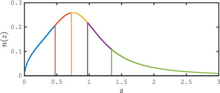
with $A=1.7865$, $a=0.4710$, $b=5.1843$, $c=0.7259$. This $n(z)$ is shown in Fig. 1 and is taken from Martinet et al. (2021a, b) and Harnois-Déraps et al. (2022). This sample is further split into five tomographic bins, each with a galaxy density of $n_{\rm gal}=6.0$ gal arcmin^-2 and shape noise of $\sigma_{\epsilon}=0.27$ per component. A summary of the mock survey properties is presented in Table 1. We assume a survey area of 5000 deg², which corresponds to the total area sampled by our flat-sky simulations at each cosmological nodes (see Sec. 3).

Figure 2: Cross-correlation coefficient matrix of our lensing power spectrum data vector, defined as $r_{ij}=C_{ij}/\sqrt{C_{ii}C_{jj}}$. The upper-left triangle shows the analytical calculations, while the lower-right part is estimated from the SLICS simulations (Sec. 3.1). The redshift bins increase towards the upper-right corner.

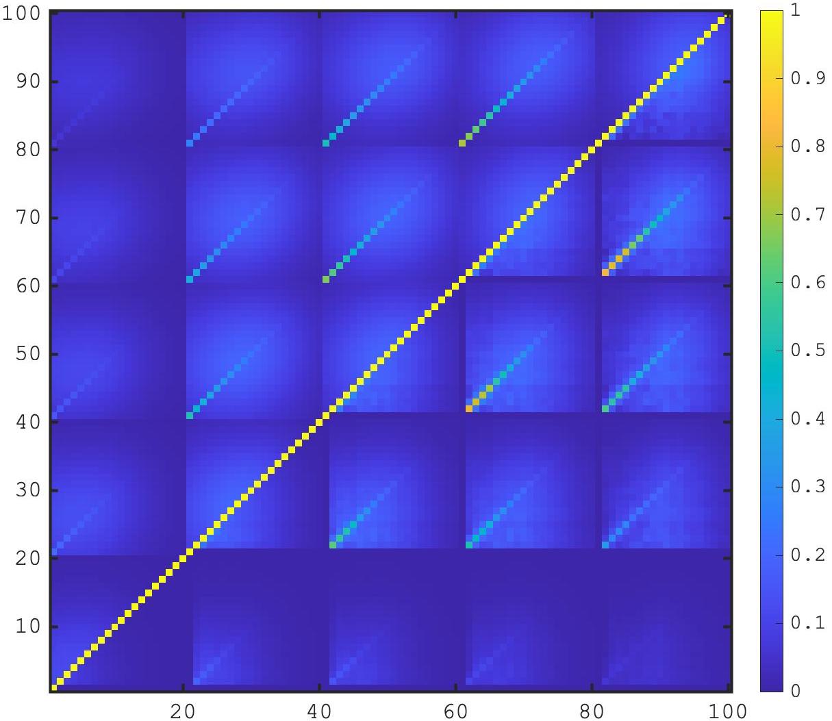
Sect. 4 details our likelihood sampling analysis, which takes as input a data vector, a covariance matrix and a theoretical model in which cosmology, gravity and nuisance parameters are varied simultaneously. As our baseline we use an analytical covariance matrix that describes the mode correlations, the shape noise and the sampling covariance expected for the different elements of our data vector. The calculations are fully detailed and validated in Harnois-Déraps et al. (2019) and Joachimi et al. (2021b) and we refer the reader to these for more information. In short they include the Gaussian, non-Gaussian and Super-Sample Covariance terms given a cosmology, a tomographic redshift distribution, a survey area and binning specifications for the angular multipoles. The non-Gaussian term requires an expensive trispectrum evaluation, while the SSC term assumes a circular survey geometry of 5000 deg². We show in Fig. 2 the cross-correlation coefficient matrix obtained with our survey specifications, and compare our results to an estimate obtained from the SLICS, which we describe in Sec. 3.1. Aside some residual noise patterns, both methods completely agree. We will quantify the impact of switching between these two later on, but basically the effect is completely subdominant given our statistical precision. This comparison validates both the theoretical approach and the SLICS maps, which will be used in companion non-Gaussian statistics studies.

3 Weak lensing simulations

The MGLenS weak lensing simulations are constructed by ray-tracing through series of mass shells obtained by collapsing the particle data either along one of the Cartesian axes (flat-sky method) or along the radial direction (curved-sky). Both methods have their pros and cons; we focus mainly on the flat-sky results in this paper for their ability to probe deeper in the small, non-linear regime, and discuss the curved-sky method in Appendix A. In either case, the mass sheets have a comoving thickness equal to exactly half the simulation box size (i.e. 250 $h^{-1}$Mpc), and between 15 and 23 shells are needed to continuously fill the light-cones up to $z=3$, depending on cosmology. We finally produce convergence maps for the five tomographic redshift bins shown in Fig. 1. In this paper we do not train our emulator on statistics measured from these maps and instead aim for their validation, however this logical extension will be presented in companion papers.

3.1 Weak lensing maps and power spectra

Figure 3: Fractional error between the emulated lensing power spectrum and that measured from the forge (upper) and bridge (lower) simulations. The grey lines are obtained for all 50 nodes, each time averaged over the 50 light-cones (two per initial conditions). The black dashed lines indicate the $1\sigma$ statistical error expected from our mock survey. Redshift increases from left to right, and the thin horizontal lines mark the 2.5% precision target.

Our flat-sky method heavily builds from the SimulLens algorithm, the multiple-plane technique described in Harnois-Déraps & van Waerbeke (2015): at each preselected redshift, the particles from half the simulation volume are projected along the shorter direction and assigned onto a 12,288² grid. This process is repeated with the other half-volume, and for the other two Cartesian axes, such that 6 density planes are extracted per snapshot.

Light-cone mass maps, $\delta_{2D}(\boldsymbol{\theta},z_{\rm lens})$, are extracted from the density planes with an opening angle of 10 deg² and $7745^{2}$ pixels. At each redshift, one of the 6 aforementioned planes is randomly selected and a random origin offset is added. This means that correlations between different mass shells are broken, but it was shown in Zorrilla Matilla et al. (2020) that this has a subdominant effect on weak lensing statistics due to the line-of-sight projection. Closely following Harnois-Déraps et al. (2019), we repeat this whole ray-tracing procedure in order to create 25 pseudo-independent light-cones $\delta_{2D}(\boldsymbol{\theta},z_{\rm lens})$ maps from each $N$-body run. Periodic boundary conditions are used wherever the area of the light-cone becomes larger than the simulation box itself.

In the multiple-plane approximation, each of these mass shells acts as a discrete gravitational lens, distorting the light as it passes through it. Within the Born approximation, the convergence $\kappa$ experienced by photons propagating along the direction $\boldsymbol{\theta}$ and originating from a source redshift distribution $n(z)$ can be computed as:

$$\kappa^{i}({\boldsymbol{\theta}})=\sum_{{\rm lens}}\delta_{2D}(\boldsymbol{\theta},z_{\rm lens})\,\,q^{i}\left(\chi(z_{\rm lens})\right)\,,$$ (20)

where $q^{i}(\chi)$ is the tomographic lensing kernel given by Eq. (18), and the index ‘lens’ runs over all foreground lens planes in the light-cone.

The cosmic shear power spectra are estimated from the square of the Fourier-transformed convergence map, first averaged in annuli of thickness $\Delta\ell=35$ centred on $\ell\in[35-5000]$:

$$C_{\ell}^{\kappa,ij}=\langle\kappa^{i}({\boldsymbol{\ell}})\kappa^{j}({\boldsymbol{\ell}})\rangle_{d\Omega}\,,$$ (21)

with $\langle...\rangle_{d\Omega}$ denoting an angular average over the solid angle of the annulus. Our measurements are then rebinned into 25 logarithmically-spaced bands over the same $\ell$-range to further reduced the sampling noise. We refer the reader to Harnois-Déraps & van Waerbeke (2015) for more details on the numerical implementation of our lensing power spectrum estimation method, which includes a mass-assignment de-biasing step; we have also checked that our measurements are consistent with those using the public code LensTools (Petri, 2016). Our fiducial cosmological inference excludes $\ell<150$ modes as these are not well measured on our 10$\times$10 deg² patches, and are affected by the finite lens thickness. The high-$\ell$ limit is an optimistic scenario, since in the real Universe these multipoles are plagued with systematic effects such as baryonic feedback, which are difficult to model and largely uncertain (Chisari et al., 2018). We therefore consider as well a more conservative scenario that further excludes the $\ell>3000$ modes. Note that we only extract the auto-angular power spectra in this work, however it is straight-forward to extend this to include cross-redshift terms as well.

3.2 Validation

Figure 4: Ratio between the tomographic weak lensing power spectrum of different forge models and that of model-00. Redshift increases from left to right, as indicated above the upper panels. Measurements from MGLenS are shown by the thin black lines, predictions from the forge emulator are indicated by the solid red lines, while the pair of thick dashed lines indicate the $\pm 1\sigma$ statistical uncertainty expected from our mock Stage-IV lensing survey. We also plot with the thin dashed red lines the GR predictions from Halofit at these cosmologies. The bridge simulations and predictions reach a similar level of agreement.

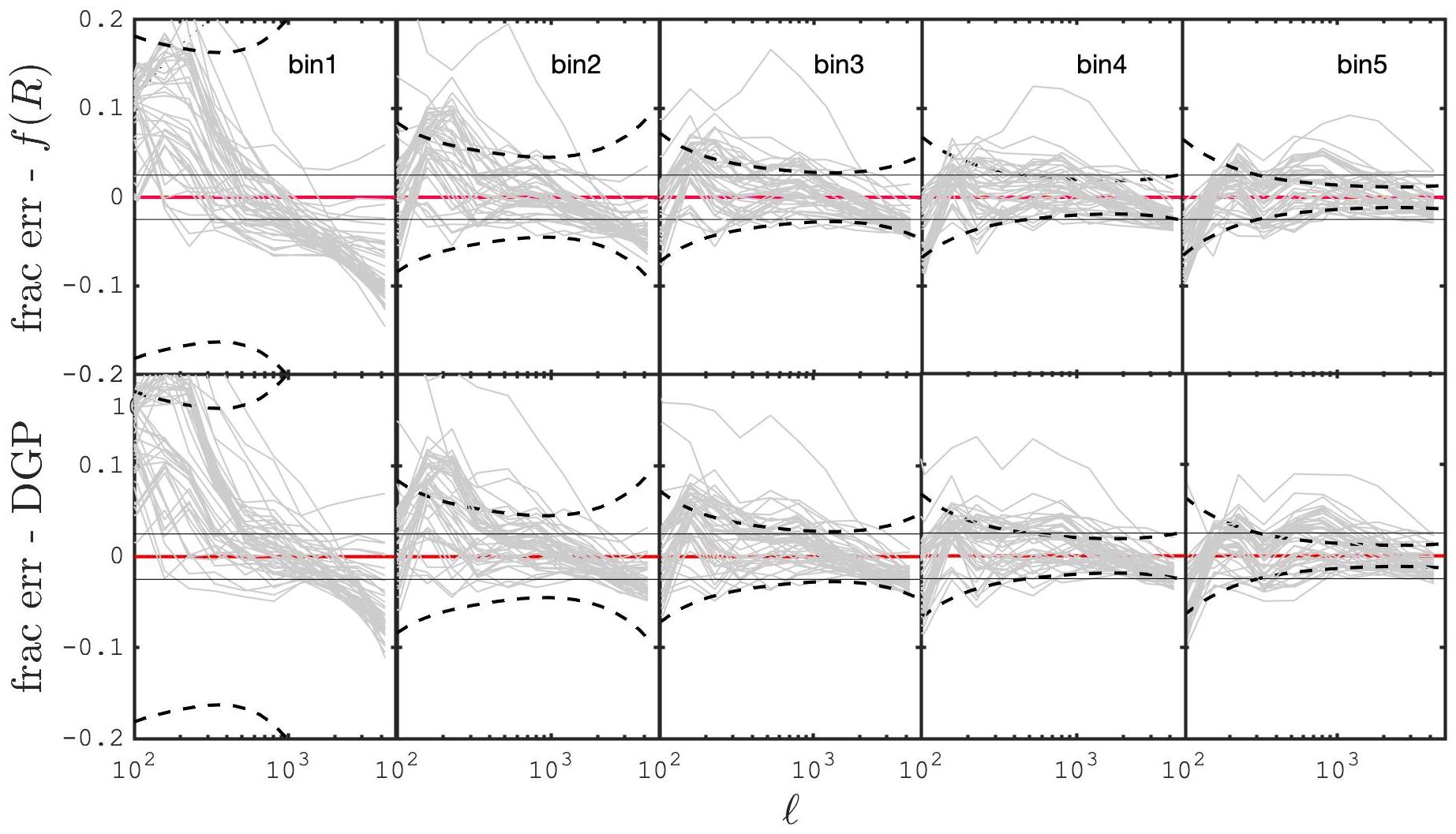
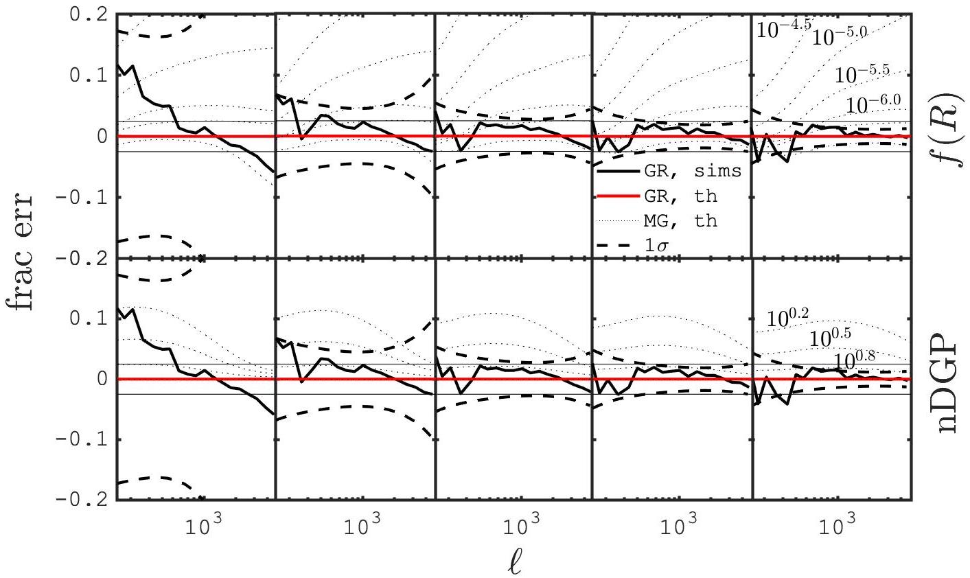
As a first validation test, we examine the fractional error between the $C_{\ell}$ measured from the forge and bridge simulations and their respective emulator predictions. We can see in Fig. 3 that the agreement is generally at the few percent level except for the lowest redshift bin, where the deviations are much larger. These are caused by reduced accuracy in the multiple lens approximation, combined with flat-sky projection effects and broken correlations, yielding tilted residuals in the left-most panel. Note that however large this might seem, the precision of lensing surveys is massively reduced at low redshifts, as seen by the black dashed lines, such that these differences should not lead to noticeable biases at the inference stage. On small scales (large $\ell$-modes) most of the measurements scatter inside the 2.5% region, consistent with the advertised 2.5% accuracy on the power spectrum emulator reported in A21. The intermediate scales (300 $<\ell<1000$) exhibit a larger scatter reaching $\sim 5\%$ at times, caused by limits in the emulator predictions combined with a small amount of residual sampling variance. From this we can expect that emulation of weak lensing statistics from these simulations should also reach 2-3% absolute accuracy.

Figure 5: top: Comparison between the lensing measurements on model-00 (black solid) relative to GR-theory (red solid), along with the expected error from the Stage-IV survey (dashed black), augmented with predictions for many $f(R)$ models (thin dotted). As before, redshift bins increases from left to right. (bottom:) Same as top panels, but now the dotted lines show nDGP model with different values of $H_{0}r_{c}$.

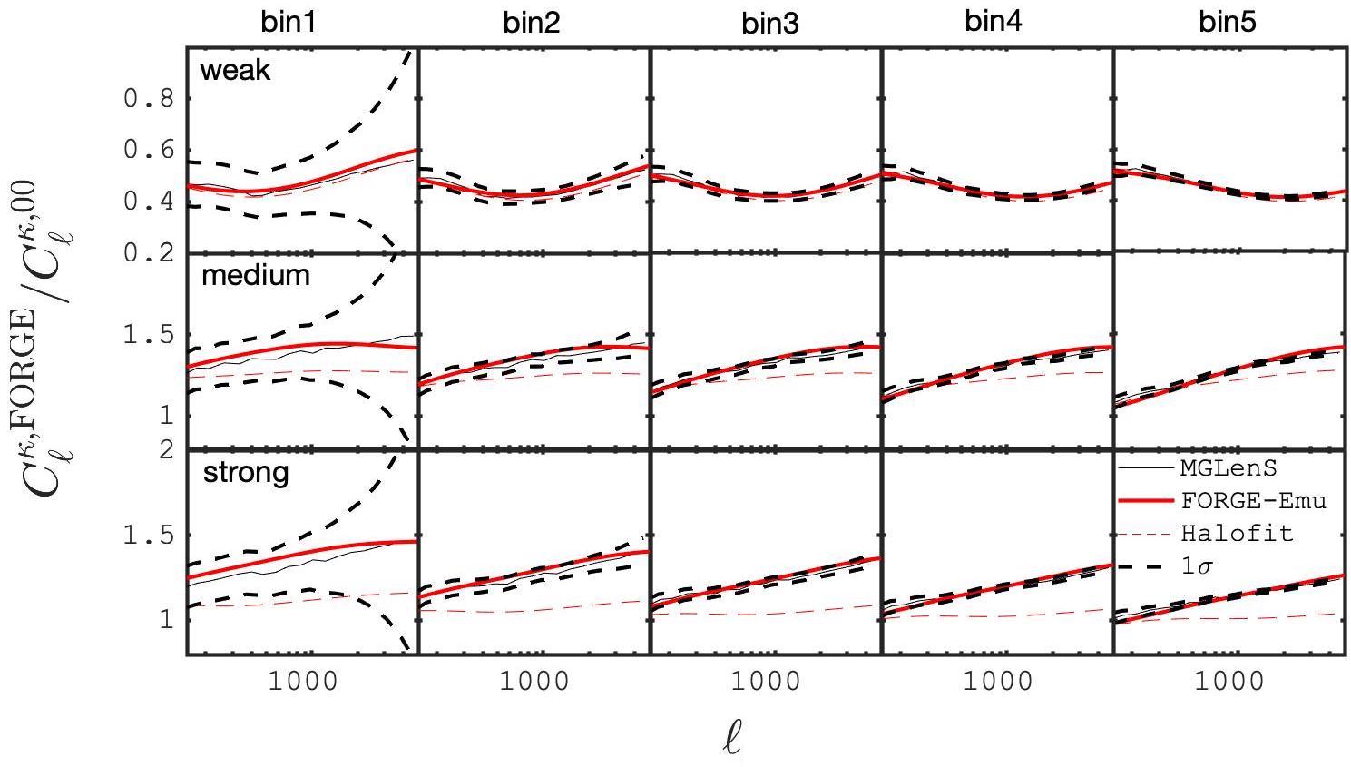
We next examine the cosmological dependence of the measurements in comparison with the emulators, shown in Fig. 4 for a representative sample of forge models. These are labelled as strong (model-13), medium (model-18) and weak (model-04), referring to the strength of their departure from GR. The match is excellent here and for most other cases; discrepancies occur only for a handful of nodes with exceptionally low $\Omega_{\rm m}$, which are poorly modelled by HaloFIT and by the forge emulator. This is well documented in A21 and is not expected to affect our cosmology and gravity inference results, which are all centred on larger values of the matter density. The emulator predictions (in red solid) is generally within the statistical precision of our mock survey (shown with the dashed black lines) for $\ell<1000$, beyond which it occasionally deviates by a few percent. This is caused by residual inaccuracies in the forge emulator itself, which was reported in A21 (see their figure 5) to emulate the simulated matter power spectrum only to a few percent precision. Similar agreements are found for all other forge and bridge models, which validates both the cosmology dependence of the light-cones and the cosmoSIS implementation of the two MG emulators.

Also shown in Fig. 4 are the predictions for the pure GR case (see the thin red-dashed curve), obtained by setting $B(k,z)=1.0$ while keeping the cosmology unchanged. The difference with respect to the solid red line is solely due to the absence of the fifth force, and falls well outside the statistical error for most models. In other words, in absence of observational and astrophysical systematics that are not included in this figure, deviations from GR would likely be observed to a high significance in our survey, if the Universe followed either the medium or strong forge models. This raises a key question: given our mock survey, how weak could be detectable deviations from GR, if they exist? The first step in answering this is to understand what redshift and angular scales mostly contribute towards such a measurement, an exercise that we carry out next with a Fisher analysis.

3.3 Fisher information

Figure 6: Fisher information as a function of $\ell_{\rm max}$, the highest mode included in the data vector, shown here for different selections of tomographic bins. The top and bottom panels are for $f_{R_{0}}$ and $H_{0}r_{c}$, respectively.

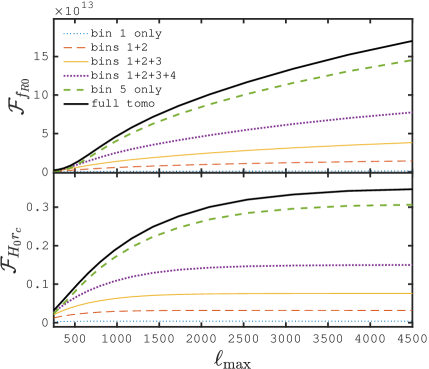
The origin of the constraining potential on $f_{R_{0}}$ and $H_{0}r_{c}$ from measurements of the lensing power spectrum is best understood by first fixing the cosmology in the emulators and varying only the modified gravity parameter. This is shown in Fig. 5 for cosmology otherwise identical to model-00, where we compare the measurements from the flat-sky GR-$\Lambda$CDM simulations (solid black) to the forge and bridge predictions with different values of their MG parameters (the thin dotted lines). Also shown are the expected statistical uncertainty. This figure suggests that the information about the $f_{R0}$ parameter mostly comes from the high redshift and high-$\ell$ modes, where the deviations with respect to GR are amplified and the statistical error bars vastly reduced. In comparison, the constraints on $H_{0}r_{c}$ arise from larger scales as well, again with the strongest detection potential coming from the highest redshift bins. This difference is driven by the type of fifth forces and screening mechanisms. In this section we dissect these signals and shine light on the data elements that better contribute to their constraints.

We carry out this investigation with a Fisher analysis (see, e.g. Takada & Jain, 2009, for a similar Fisher matrix calculation), which is cheaper to run than a full MCMC while providing exactly the information we are seeking. Given measurements of the lensing power spectrum, the Fisher information about a parameter $\pi$ is obtain from

$$\mathcal{F}_{\pi}=\left[\frac{{\rm d}C_{\ell}}{{\rm d}\pi}\right]{\rm Cov}^{-1}\left[\frac{{\rm d}C_{\ell}}{{\rm d}\pi}\right]^{\rm T}\,,$$ (22)

where Cov is the covariance matrix shown in Fig. 2, which we assume to be cosmology independent in our calculation. A matrix product is taken between the three terms, resulting in a single scalar quantity per parameter $\pi$. In short, the contribution to the information is large for elements of the data vector that are highly sensitive to changes in $\pi$ (i.e. their derivative is large) and for which the covariance is small (the inverse is large). The inverse of $\mathcal{F}$ provides an optimistic estimate of the covariance about $\pi$, which in our one-dimensional case gives $\sigma_{f_{R0}}=\sqrt{\mathcal{F}_{f_{R0}}^{-1}}$ and $\sigma_{H_{0}r_{c}}=\sqrt{\mathcal{F}_{H_{0}r_{c}}^{-1}}$.

Starting our dissection, we compute the Fisher information for different selections of the full data vector, first allowing variations in the maximal multipole included in our survey, $\ell_{\rm max}$. The results are shown in Fig. 6 with the solid black line, where for $f_{R_{0}}$ we observe that the increase in information remains significant for all scales included here. We notice a slight transition past $\ell_{\rm max}=1500$ where the slope becomes shallower, due to the non-linear coupling between the different Fourier modes (Takada & Jain, 2009). The flattening of the slope is more pronounced for $H_{0}r_{c}$, where a full information saturation is observed beyond $\ell=3000$, similar to that found by Takada & Jain (2009, see their figure 3).

We next explore the impact of adding each of the tomographic bins one at a time. The second line from the top shows the information contained solely in the highest tomographic bin, while the other lines correspond to different combinations of the lower redshift bins. It is clear from this that most of the information is contained in bin 5, the other four bins providing only a modest additional gain.

Using all scales and all tomographic bins, we could expect a detection of at least $3\sigma$ if $f_{R0}>2.3\times 10^{-7}$ or if $H_{0}r_{c}<5.1$, in absence of systematics and assuming that the cosmology is perfectly known from external data. We could include variations with cosmology and marginalisation over systematics in an upgraded Fisher calculation, however we choose instead to run full MCMC on mock data, yielding the most accurate picture of the inference capabilities provided by the MGLenS simulations.

4 Cosmology Inference

Table 2: Priors used in our cosmological inference. Except for $\delta z^{i}$, all parameters are sampled with a uniform (i.e. flat) prior; a Gaussian prior of width 0.01 is applied on the redshift parameters, reflecting a realistic precision we should have on the redshift distributions.

parameter	range
$\Omega_{\rm m}$	0.1 – 0.55
$S_{8}$	0.6 – 0.9
$h$	0.6 – 0.82
log${}_{10}[f_{R_{0}}]$	-8.0 – -4.5
log${}_{10}[H_{0}r_{c}]$	-0.6 – 1.0
$A_{\rm IA}$	-5.0 – 5.0
$\delta z^{i}$	-0.1 – 0.1

This section presents the inference method with which we quantify our ability to distinguish cosmological and gravitational parameters in different scenarios. After validating our inference pipeline, we run a sensitivity test on both MG models, this time varying both cosmological and gravity parameters. We next validate the measurements from the MGLenS simulations, then investigate the catastrophic impact of analysing mock MG data with the wrong gravity model, thereby demonstrating the strong model-dependence of this approach. We finally study the impact of various systematics effects on these measurements. Our data vector consists once again of the auto-spectra measured from the weak, medium and strong forge/bridge models in all five tomographic bins.

In all cases our likelihood assumes a standard multivariate Gaussian functional form with a fixed covariance matrix (see Section 2.5). The predictions are computed at arbitrary cosmologies using Eq. 17 augmented with the $B(k,z)$ emulators, with a flat prior on the four parameters ($\Omega_{\rm m}$, $S_{8}$, $h$ and either log${}_{10}[f_{R_{0}}]$ or log${}_{10}[H_{0}r_{c}]$) that spans the range for which the emulators are supported, listed in Table 3. One exception to this is the lower bound on log${}_{10}[f_{R_{0}}]$ which we set to $-8$ in order to reduce prior effects in the weak MG limit. Otherwise the inference pipeline could wrongly reject log${}_{10}[f_{R_{0}}]\sim-7$ simply because it is poorly sampled. As explained before, we set $B(k,z)$ to 1.0 whenever log${}_{10}[f_{R_{0}}]\in[-8,-7]$. The other cosmological parameters are held fixed to the values used in the $N$-body runs.

We carry out our cosmology inferences with the likelihood sampler Multinest (Feroz et al., 2009), which is run within cosmoSIS. This sampling method has been used and validated in a number of previous works, notably in the cosmic shear analysis of the KiDS-1000 data (Asgari et al., 2021) and of the DES-Year 3 data (Secco et al., 2021). It has been reported in Lemos et al. (2022) that the projected contours could be slightly over-constraining in some cases compared to alternative samplers, however we opted for Multinest as it is much faster and its accuracy is sufficient to support the scientific goals of this paper. The chains all ran in 5000 steps and are analysed with getdist.

4.1 Likelihood-based forecasts on $f_{R_{0}}$ and $H_{0}r_{c}$

Figure 7: Marginalised constraints on the forge (upper panel) and bridge (lower) parameters when analysing cosmology-00 in which the input data is taken directly from theory predictions, for three values of log${}_{10}\left[f_{R_{0}}\right]$ and log${}_{10}\left[H_{0}r_{c}\right]$ indicated in the legend.

Forecasts on weak lensing $f_{R_{0}}$ and $H_{0}r_{c}$ constraints found in the literature need to be revisited, mostly due to recent improvements in modelling the deep non-linear matter power spectrum in presence of a screened fifth force. For example, Pratten et al. (2016) forecast that with a full-sky 3D weak lensing analysis based on spectroscopic data, and assuming that the cosmological background is fixed by CMB data, one could constrain $f_{R_{0}}<5\times 10^{-6}$. Their $\chi^{2}$ analysis is simpler than our full MCMC approach, they used a hybrid one-loop perturbation theory and halo-model to compute the $P(k)$ in presence of MG, and unlike us they do not include WL systematics. Other examples include the Euclid forecast of Thomas et al. (2009) that predicts from a Fisher analysis that the nDGP signal will be clearly detectable from lensing alone. Martinelli et al. (2011) and Casas et al. (2017) also predicts clear detection of MG signal from Euclid, this time using MGcamb (Hojjati et al., 2011) for the $P(k)$ modelling, including $\ell$-modes up to 5000, and assuming the commonly used $(\mu,\Sigma)$ phenomenological parameterisation. None of these adequately investigate the sensitivity of modern cosmic shear surveys, which we here begin to address.

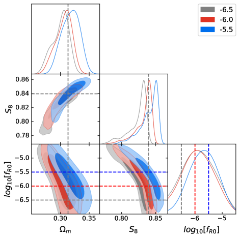
Fig. 7 (top panel) presents the posterior distributions from three likelihood samplings, in which the data is taken directly from the forge emulator predictions, at cosmology-00 and for log${}_{10}\left[f_{R_{0}}\right]=-6.5,-6.0$ and $-5.5$. We observe a strong degeneracy between $f_{R_{0}}$ and $S_{8}$, expected from the fact that these two parameters both modulate the overall amplitude of the lensing signal. This degrades the constraining performance with respect to our previous Fisher calculation (Sec. 3.3). If $S_{8}$ was fixed, we could indeed detect with high significance these three models (imagine slicing through the $S_{8}-f_{R_{0}}$ contours along the vertical dashed line at the input $S_{8}$ value), however the two weakest models are hitting the GR-limit when $S_{8}$ becomes large. The $f_{R_{0}}=10^{-5.5}$ model, on the other hand, would be detected at the $\sim\!3\sigma$ level. This is an order of magnitude less constraining that what was found by our one-dimensional Fisher forecast, but is more realistic as we are now fully including gravity-cosmology degeneracies.

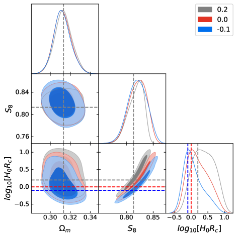
The lower panel of Fig. 7 shows a similar exercise carried out on nDGP data taken directly from the bridge emulator. We observe that in all cases the three parameters are correctly inferred, and that the $[S_{8}-H_{0}r_{c}]$ degeneracy direction is inverted compared to $f_{R_{0}}$ due to the fact that in this model strongest deviations occur for smaller $H_{0}r_{c}$ values. Finally, whereas the posterior from weakest nDGP model in this figure (grey contours, corresponding to log${}_{10}\left[H_{0}r_{c}\right]=0.2$) is prior-dominated towards the higher $H_{0}r_{c}=$ bound, the other two models are not: $H_{0}r_{c}<1.0$ could be detected beyond $3\sigma$ in this forecast. Once again this error is less constraining than our Fisher forecast, as expected from the added realism. Fixing cosmology would significantly help in this measurement as well, as the posteriors are narrow along a fixed $S_{8}$ value.

4.2 Recovering the GR-$\Lambda$CDM simulation

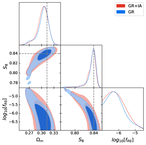
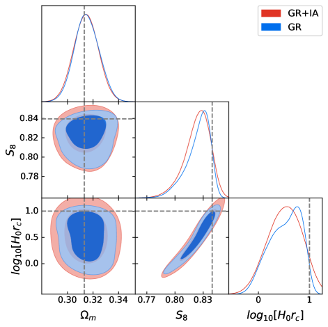
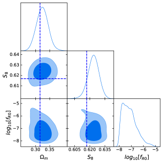
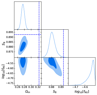
Fig. 8 presents our first inference validation test on the MGLenS simulations, where we run our analysis pipeline on the GR-only model, assuming consecutively a forge and bridge gravity model (top and bottom panels, respectively). It is important to note here that our noise-free data has been measured from 5000 deg², and our analytical covariance matrix assumes the same area and includes shape noise. We therefore expect the input truth to lie close to the center of the $1\sigma$ regions, but offset can be caused by residual sampling variance in the mocks and interpolation errors from the emulators. This is indeed consistent with what we observe in Fig. 8, establishing that we correctly infer the input cosmological parameters, and prefer modified gravity models that are beyond detection, with:

$${\rm log}_{10}\left[f_{R0}\right]<-5.08\,,$$

and

$${\rm log}_{10}\left[H_{0}r_{c}\right]>-0.051\,,$$

in absence of systematics (both upper limits are reported with 95%CL). Note that these one-sided limits depend on the prior range we adopt: larger sampled volumes (on the weak MG side) down-weight the tails and hence artificially increase the constraining power. For example, truncating the MCMC chains at ${\rm log}_{10}\left[f_{R0}\right]$=[$-7.0$,$-7.5$,$-8.0$] yield upper limits of [$-4.96$, $-5.08$ and $-5.24$], respectively. We selected the middle value in this work, but care must be taken when comparing these results with others found in the literature. Note that the results obtained here seems to contradict Fig. 5, in which models with $f_{R_{0}}>10^{-6.0}$ clearly stand out of the 2$\sigma$ region at high-redshift, but again, this observation is ignoring the $[f_{R_{0}}-S_{8}]$ degeneracy.

An important feature of this figure is that the degeneracy between $f_{R_{0}}$ and $S_{8}$ vanishes when sampling lower $f_{R_{0}}$ values, as seen in the lower part of the contours which are close to vertical; this is also seen in Fig. 7. That is likely due to the fact that a small $f_{R_{0}}$ tends to have little modification to the clustering in the linear regime on large scales, where the amplitude of clustering is influenced by $S_{8}$ more directly; instead, it tends to cause stronger deviations to its GR counterpart only at the very small scales, where there is also a stronger nonlinearity, thus a weaker connection to the amplitude parameter $S_{8}$. Put together, these two factors, the relatively stronger effect of $f_{R_{0}}$ on small scales and stronger nonlinearity, naturally break the degeneracy between $f_{R_{0}}$ and $S_{8}$ when $f_{R_{0}}$ is small. This is not the case for other forge models with a stronger MG sector, as we will see in the following section.

For nDGP, shown on the bottom panel of Fig. 8, the degeneracy with $S_{8}$ is present at every value of $H_{0}r_{c}$, even for weak deviations from GR, but the input cosmology is well recovered, even though this model is at the edge of the Latin Hypercube.

Figure 8: Marginalised constraints on the forge (upper) and bridge (lower) parameters when analysing the GR simulations. Given our prior limits and the important degeneracy between $S_{8}$ and the MG parameters, we recover the expectation that the input truth is well inside the $1\sigma$ contours, but not necessarily at the center.

Figure 9: Marginalised constraints on the forge (left) and bridge (right) parameters, for models-04 (upper panels, weak MG), -18 (middle panels, medium MG) and -13 (lower panels, strong MG). No systematics are included here.

Figure 10: Marginalised constraints on the two composite parameters introduced in this paper, $\zeta_{R_{0}}^{\alpha}$ and $\zeta_{r_{c}}^{\alpha}$ (see Eqs. 23 and 24), which are best measured by cosmic shear data when cosmology and modified gravity parameters are jointly varied. These are extracted at the weak $f(R)$ (left) and medium nDGP (right) gravity models.

4.3 Recovering the forge and bridge simulations

Table 3: Measurements of the modified gravity parameters inferred from the tomographic weak lensing power spectrum analysis of the forge and bridge simulations. We show the results for a selection of models (top to bottom show GR, $f(R)$ and nDGP gravity). The last column shows the impact of marginalising over the $A_{\rm IA}$ nuisance parameter. In our forge and bridge emulators, the GR node is taken at log${}_{10}\left[f_{R0}\right]=-7.0$ and log${}_{10}\left[H_{0}r_{c}\right]=1.0$, respectively. Upper and lower limits are reported at 95%CL.

model	parameter	truth	no-syst	IA
GR	$\Omega_{\rm m}$	$0.313$	$0.315^{+0.010}_{-0.010}$	$0.314^{+0.009}_{-0.009}$
	$S_{8}$	$0.840$	$0.834^{+0.011}_{-0.003}$	$0.834^{+0.011}_{-0.003}$
	log${}_{10}\left[f_{R0}\right]$	$-\infty$	$<-5.08$	$<-5.24$
	log${}_{10}\left[H_{0}r_{c}\right]$	$\infty$	$>-0.05$	$>-0.05$
forge-weak	$\Omega_{\rm m}$	$0.316$	$0.319^{+0.022}_{-0.025}$	$0.318^{+0.023}_{-0.027}$
	$S_{8}$	$0.617$	$0.618^{+0.008}_{-0.007}$	$0.618^{+0.008}_{-0.007}$
	log${}_{10}\left[f_{R0}\right]$	$-6.09$	$-6.69^{+0.67}_{-1.00}$	$-6.74^{+0.64}_{-1.00}$
	$\zeta_{R_{0}}$	-25.3	$-27.5^{+3.9}_{-2.3}$	$-27.7^{+3.9}_{-2.5}$
forge-medium	$\Omega_{\rm m}$	$0.323$	$0.313^{+0.010}_{-0.010}$	$0.310^{+0.010}_{-0.010}$
	$S_{8}$	$0.893$	$0.883^{+0.018}_{-0.007}$	$0.879^{+0.018}_{-0.016}$
	log${}_{10}\left[f_{R0}\right]$	$-5.43$	$-5.13^{+0.22}_{-0.33}$	$-5.05^{+0.36}_{-0.32}$
	$\zeta_{R_{0}}$	-3.55	$-3.55^{+0.14}_{-0.06}$	$-3.57^{+0.13}_{-0.11}$
forge-strong	$\Omega_{\rm m}$	0.347	$0.360^{+0.014}_{-0.026}$	$0.361^{+0.021}_{-0.021}$
	$S_{8}$	0.841	$0.858^{+0.020}_{-0.014}$	$0.858^{+0.020}_{-0.013}$
	log${}_{10}\left[f_{R0}\right]$	$-4.90$	$-5.25^{+0.59}_{-0.39}$	$-5.26^{+0.58}_{-0.46}$
	$\zeta_{R_{0}}$	-4.33	$-4.18^{+0.15}_{-0.10}$	$-4.19^{+0.20}_{-0.15}$
bridge-weak	$\Omega_{\rm m}$	$0.316$	$0.316^{+0.022}_{-0.022}$	$0.314^{+0.020}_{-0.023}$
	$S_{8}$	$0.617$	$0.617^{+0.009}_{-0.009}$	$0.617^{+0.009}_{-0.009}$
	log${}_{10}\left[H_{0}r_{c}\right]$	$0.602$	$0.53^{+0.34}_{-0.25}$	$0.53^{+0.30}_{-0.27}$
	$\zeta_{r_{c}}\times 10^{3}$	0.36	$0.40^{+0.14}_{-0.38}$	$0.39^{+0.16}_{-0.37}$
bridge-medium	$\Omega_{\rm m}$	$0.323$	$0.322^{+0.008}_{-0.008}$	$0.321^{+0.007}_{-0.007}$
	$S_{8}$	$0.893$	$0.886^{+0.013}_{-0.007}$	$0.885^{+0.012}_{-0.009}$
	log${}_{10}\left[H_{0}r_{c}\right]$	$-0.163$	$-0.24^{+0.10}_{-0.07}$	$-0.26^{+0.08}_{-0.08}$
	$\zeta_{r_{c}}$	-1.478	$-1.75^{+0.26}_{-0.26}$	$-1.76^{+0.23}_{-0.23}$
bridge-strong	$\Omega_{\rm m}$	0.347	$0.343^{+0.008}_{-0.008}$	$0.339^{+0.006}_{-0.006}$
	$S_{8}$	0.841	$0.849^{+0.013}_{-0.011}$	$0.846^{+0.012}_{-0.012}$
	log${}_{10}\left[H_{0}r_{c}\right]$	$-0.443$	$-0.40^{+0.10}_{-0.10}$	$-0.42^{+0.12}_{-0.14}$
	$\zeta_{r_{c}}$	-0.845	$-0.98^{+0.11}_{-0.16}$	$-0.92^{+0.12}_{-0.12}$

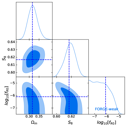
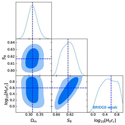
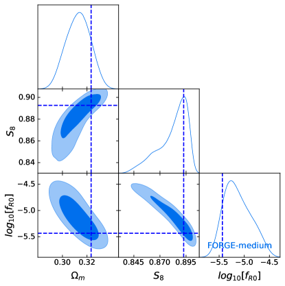
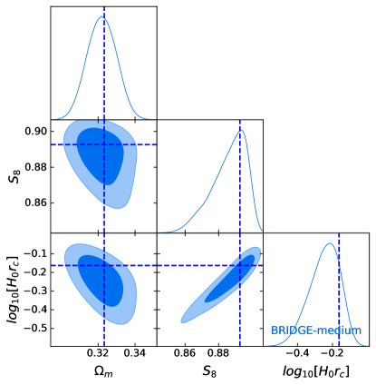
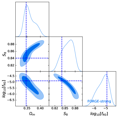
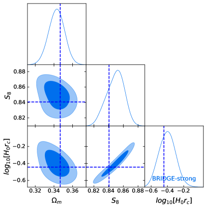
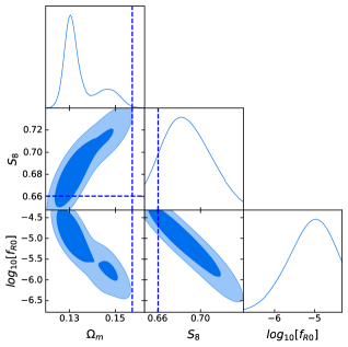
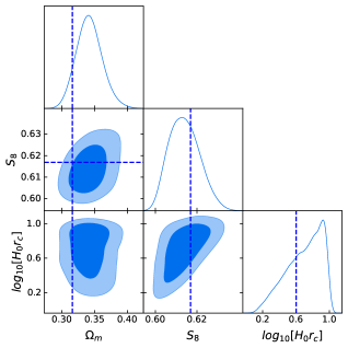
We now turn our attention to other MGLenS nodes, with Fig. 9 showing the inferred parameters when analysing a series of forge and bridge data vectors (left and right panels, respectively), specifying the correct gravity framework ($f(R)$ or DGP) at the moment; we investigate later the result of specifying the wrong framework. We present, from top to bottom, models with increasing deviations from GR. Once again the input cosmologies are recovered within $1\sigma$, which validates both the MGLenS simulations and the cosmoSIS implementation of the forge and bridge emulators in our end-to-end cosmological inference. One of the most important features seen here is the strong degeneracy between the MG parameters ($f_{R_{0}},H_{0}r_{c}$) and $S_{8}$. Looking now at the posteriors, according to these results, if the gravitational physics of our Universe matched the medium or strong models in these survey conditions, we could strongly rule out GR and constrain the MG sector with our survey. The marginalised posteriors on the parameters of interests are summarised in Table 3, where, for example, our measurement for the weak forge yields log${}_{10}\left[f_{R0}\right]=-6.69^{+0.67}_{-1.00}$, which is fully consistent with the input truth (-6.09). Similar results can be seen for the nDGP inference analyses, where the large values of $H_{0}r_{c}$ are heavily disfavoured, while successfully recovering the input simulation values.

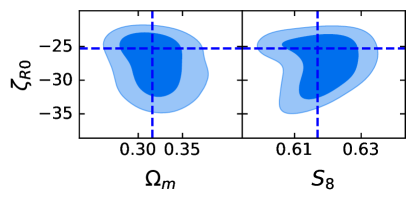
The observed [$f_{R_{0}},S_{8}$] degeneracy limits the precision we can achieve on these two parameters separately, which incites us to define a combination that is better measured. Inspired by the $\Sigma_{8}\equiv\sigma_{8}(\Omega_{\rm m}/0.3)^{\alpha}$ composite lensing parameter, we introduce a new variable which runs across the minor axis of the degeneracy ellipse:

$$\zeta_{R_{0}}^{\alpha}\equiv\mbox{ log}_{10}\left[f_{R_{0}}\right]\left(\frac{S_{8}}{0.82}\right)^{\alpha}\,,$$ (23)

where $\alpha$ is a free parameter to be optimised. For small values of $f_{R_{0}}$, $\alpha=5.0$ returns a $\zeta_{R_{0}}^{\alpha}$ that is mostly orthogonal to both $S_{8}$ and $\Omega_{\rm m}$, making this an attractive target measurement for future cosmic shear experiments. We post-pone to future work the impact of letting $\alpha$ free in a likelihood analysis.

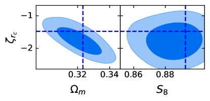
The equivalent degeneracy-breaking parameter for nDGP models can be constructed as

$$\zeta_{r_{c}}^{\alpha}\equiv\mbox{ log}_{10}\left[H_{0}r_{c}\right]\left(\frac{S_{8}}{0.82}\right)^{\alpha}\,,$$ (24)

where $\alpha=26$ works better for the nDGP models. We show in Fig. 10 the marginalised constraints on these two new parameters, $\zeta_{R_{0}}^{\alpha}$ and $\zeta_{r_{c}}^{\alpha}$, where the degeneracy with respect to $S_{8}$ and $\Omega_{\rm m}$ is highly suppressed. The accuracy on these composite parameters is increased, where for example a 9% measurement of log${}_{10}\left[f_{R_{0}}\right]$ results in a 3% precision on $\zeta_{R_{0}}^{\alpha}$ in the strong forge model. Similar improvements are seen on nDGP parameters, where a 25% measurement of log${}_{10}\left[H_{0}r_{c}\right]$ becomes a 14% measurement of $\zeta_{r_{c}}^{\alpha}$ in the strong bridge model. The measurements reported in Table 3 indicate a net gain in precision for all models.

By construction, the variables $\zeta_{R_{0}}^{\alpha}$ and $\zeta_{r_{c}}^{\alpha}$ down-weight parameter regions of weak modified gravity, which therefore interacts with prior limits. These parameters are therefore mostly useful for medium and strong modified gravity models, but we advise against using them for one-sided limits.

Figure 11: (Upper:) Marginalised parameter constraints when analysing forge simulations (left is weak model, center is medium, right is the strong model-05) with the bridge emulator, yielding to catastrophic biases. (Lower:) Counterpart of the upper panels, now analysing bridge simulations with the forge emulator.

4.4 Degeneracies between gravity models and cosmology

Table 4: Impact of analysing MG simulated data with the wrong gravity model. Column $\Lambda$CDM+GR shows the results of analysing MGLenS simulations with a GR model (i.e. Halofit), while the ‘Wrong MG’ columns consider forge data analysed with the bridge emulator and vice versa. The parameter shift are computed as $|$bestfit - true$|/\sigma$, and the $p$-values assume four free parameters.

True		True model		$\Lambda$CDM+GR		Wrong MG
gravity model	param	shift	$p$-value	shift	$p$-value	shift	$p$-value
forge-weak	$\Omega_{\rm m}$	0.7$\sigma$	1.0	$1.1\sigma$	1.0	$1.4\sigma$	1.0
	$S_{8}$	0.4$\sigma$		$0.3\sigma$		$0.4\sigma$
forge-medium	$\Omega_{\rm m}$	0.4$\sigma$	0.77	$23.7\sigma$	0.0	$11.3\sigma$	0.0
	$S_{8}$	0.8$\sigma$		$12.8\sigma$		$6.9\sigma$
forge-strong	$\Omega_{\rm m}$	1.8$\sigma$	1.0	$4.3\sigma$	1.0	$8.2\sigma$	0.997
	$S_{8}$	0.7$\sigma$		$17.6\sigma$		$13.4\sigma$
bridge-weak	$\Omega_{\rm m}$	0.7$\sigma$	1.0	$0.6\sigma$	1.0	$0.4\sigma$	1.0
	$S_{8}$	0.2$\sigma$		$1.2\sigma$		$1.2\sigma$
bridge-medium	$\Omega_{\rm m}$	0.2$\sigma$	0.97	$8.5\sigma$	0.0	$10.8\sigma$	0.0
	$S_{8}$	2.0$\sigma$		–		$3.7\sigma$
bridge-strong	$\Omega_{\rm m}$	1.0$\sigma$	1.0	$5.3\sigma$	0.002	$2.2\sigma$	0.003
	$S_{8}$	2.1$\sigma$		$20.7\sigma$		$1.2\sigma$

One of the main difficulties in detecting deviations from GR comes from the abundance of models to be tested, which each affect the growth of structures in different ways. A key question to be answered is whether one can confuse a clear detection of gravity model ‘A’ at some cosmology with a different gravity model ‘B’ at a different cosmology. The first part of the answer is already provided in the GR-only validation test, where both the forge and bridge emulators recognise negligible deviations from GR in model-00, both inferring the right cosmology. This is encouraging since it suggests that GR can be recognised as such.

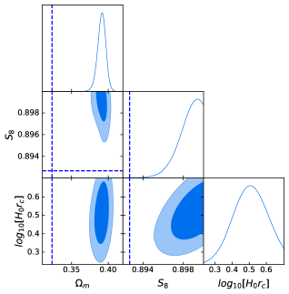
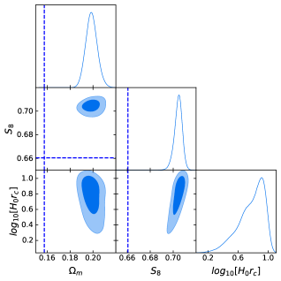
Complications arise when analysing truly non-GR data with the wrong gravity model. The upper panels of Fig. 11 shows such examples, where three forge data vectors are analysed with the bridge emulator. For the weak model (left), this results in a minor bias in $\Omega_{\rm m}$ and $S_{8}$, and a wide posterior on $H_{0}r_{c}$ that hits the upper edge prior, leading to inconclusive detection of MG. The central and right panels, however, reveal catastrophic biases on the cosmological parameters for the medium and strong models. The two cosmological parameters are shifted towards higher values, while the posteriors indicate an apparent $H_{0}r_{c}$ detection. Similarly catastrophic results are observed when, on the contrary, we analyse nDGP data with the forge emulator (see the lower panels of Fig. 11); in this case most inferred cosmological parameters are also far from the truth, and the $f_{R_{0}}$ parameter is falsely detected with high significance for both medium and strong nDGP models.

Biases also occur if data from a modified gravity universe is analysed with a GR-only model, in which case the additional structure formation caused by the fifth force is interpreted as a higher $S_{8}$ value, as expected from the degeneracy between these quantities. Table 4 summarises these parameter shifts, normalised by the precision $\sigma$. We see again that the weak models has almost no impact on the inferred cosmology (shift $\sim 1\sigma$), whereas the stronger model can offset $\Omega_{\rm m}$ by up to $23.7\sigma$ and $S_{8}$ by up to $17.6\sigma$.

This inevitably raises the question of whether we could know that we are analysing the data with the wrong gravity model. One of the standard approaches is to examine the goodness-of-fit, which informs us on the quality of the data-model match. This can be computed with the $p$-value measured at the best-fit parameters for different gravity models, from which one can test different model hypotheses. A $p$-value below 0.01 generally indicates that the hypothesis should be rejected. Table 4 presents the measured $p$-values for different combinations of models and data. In our case this test is done with noise-free data, so we expect the distributions of $p$-values to be sharply bimodal between 0.0 and 1.0. It turns out that some data (e.g. forge-04) and bridge-04 can be well fit by all three models, due to weakness of the departure from GR. GR and nDGP gravity can also provide a good fit to the forge-05 data, which is achieved at the cost of significantly increasing both $\Omega_{\rm m}$ and $S_{8}$. This bias is clearly seen in the lower-right panel of Fig. 11. One would have problems, in such a case, to distinguish between gravity models, unless augmenting the analysis with prior knowledge of the cosmological parameters from e.g. the CMB. Other test cases are easier to reject based on the bad goodness-of-fit, such as forge-18 and bridge-18, which can only be well fit with the correct gravity model.

Other metrics exist to quantify tensions between data and models such as Bayesian Evidence ratios (Hobson et al., 2002; Marshall et al., 2006) or Suspiciousness (Lemos et al., 2020), the latter being more robust to prior-effects (see also Joachimi et al., 2021a, for a recent discussion on the application of such metrics to real cosmological data). These metrics would be useful to explore as well, but have come with their own challenges and sets of requirements and hence we leave such investigations for future work.

4.5 Impact of systematics

Figure 12: Marginalised constraints on the parameters best probed by lensing, with and without including contamination from intrinsic alignment in the modelling.

Figure 13: Impact of scale cuts on the marginalised constraints, here shown for the forge strong model.

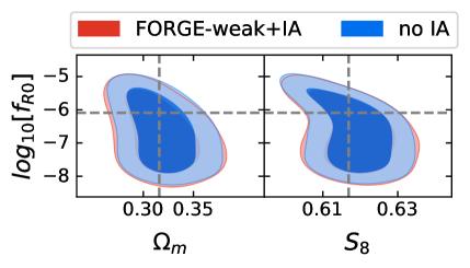
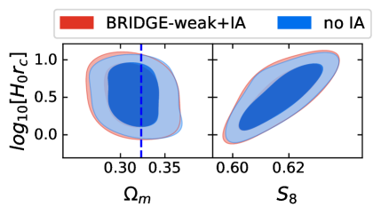
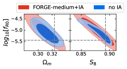
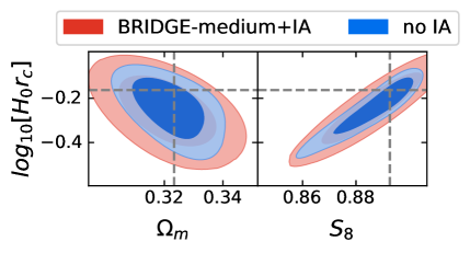
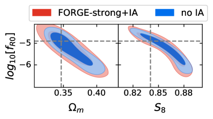
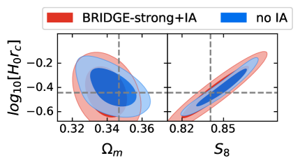
The results from the beginning of Sec. 4 are obtained in unrealistically clean conditions; as discussed previously, cosmic shear surveys are in fact affected by poorly constrained intrinsic alignments (IA), by uncertainty on the photometric redshift (photo-$z$) distributions and shape calibration, as well as by largely unconstrained baryonic feedback. Additionally the weak lensing signal is mildly sensitive to some of the other cosmological parameters such as the baryon density $\Omega_{\rm b}$, the sum of neutrino masses $\Sigma m_{\nu}$ or the tilt in the primordial power spectrum, $n_{\rm s}$, such that our constraints are likely slightly over-precise. Here we focus on two of these, namely the photo-$z$ and the IA, leaving a more comprehensive study of the others for future work. To some extent the impact of baryon can be reduced by removing some of the non-linear scales, which we also touch upon below.

Using cosmoSIS for the calculation of the theoretical cosmic shear predictions has key advantages when it comes to modelling and marginalising over the known weak lensing systematics. First, the public version includes an implementation of the widely used non-linear alignment model (Bridle & King, 2007), which describes the IA contamination from a linear coupling between the intrinsic galaxy orientations and the local tidal field. This model has been shown to accurately capture the IA signal in many cosmic shear analyses (see e.g. Asgari et al., 2021; Troxel et al., 2018), with weak signs of potential limitations in the most recent DES-Y3 analysis by Secco et al. (2021). In all cases, IA significantly bias the inferred cosmology if left unmodelled. Assuming no IA redshift evolution, the uncertainty is captured by a single scaling parameter, $A_{\rm IA}$, which we allow to vary over the range [-5.0, 5.0] in line with these previous analyses.

Second, cosmoSIS deals with the uncertainty on the redshift distribution by shifting the tomographic $n^{i}(z)$ by a constant quantity $\delta_{z}^{i}$, which we treat independently for each tomographic bin $i$: $n^{i}(z)=n^{i}(z+\delta_{z}^{i})$. It has been shown that in some cases these shift parameters are correlated (Wright et al., 2020), however we ignore this here. Our five $\delta_{z}^{i}$ parameters are sampled assuming a Gaussian prior of width 0.01, similar to the accuracy achieved by current weak lensing surveys (for example, an accuracy between 0.0084 and 0.0116 on these $\delta_{z}$ parameters is achieved with the KiDS-1000 data, see Hildebrandt et al., 2021). We do not include the uncertainty on shape calibration (i.e. the $m$-bias, see Giblin et al., 2021) as it is currently subdominant compared to the effect of IA and photometric redshift (Asgari et al., 2021; Secco et al., 2021). Importantly, we neglect the impact of baryon feedback, which is arguably the largest approximation in our analysis. Indeed, baryons significantly redistribute the matter distribution and suppress the lensing signal by tens of percent depending on the scales and baryonic physics (Semboloni et al., 2011; Harnois-Déraps et al., 2015). We could extend our results by using for instance the matter power spectrum provided by HMCode (Mead et al., 2021) in which the impact of baryons is modelled, but we leave this for future work. We finally assume a constant total neutrino mass set to $\Sigma m_{\nu}=0.0$ eV, in order to be consistent with the forge and bridge simulations. All of these analysis choices have an impact on the inference and will need to be revisited in order to make robust constraints on the MG parameters from cosmic shear data, however our simplified likelihood evaluations represent an important first step in this direction.

We show in Fig. 12 (and summarise the results in Table 3) the impact of IA on the marginalised constraints for some of the forge and bridge models. As expected, the presence of IA degrades the constraints on most parameters, where for example the 1.4% measurement of $S_{8}$ value in the forge medium model becomes a 1.9% measurement. The same model sees the constraints on log${}_{10}\left[f_{R_{0}}\right]$ degrade from a 5.4% to a 6.7% measurement. We also note that for some models (e.g. forge medium, bridge strong), the IA contamination acts mostly along the $\left[f_{R_{0}}-S_{8}\right]$ or $\left[H_{0}r_{c}-S_{8}\right]$ degeneracy directions, whereas for other models the posterior is inflated in all dimensions (e.g. forge-strong). Finally low-$S_{8}$ models appear to be less affected (e.g. forge weak), which is expected since the IA signal also scales with $S_{8}$, causing them to be harder to distinguish from the cosmological signal given our fixed covariance matrix. Also worth repeating here is that our data vector does not include any of the cross-tomographic terms, which are more affected by IA as they are highly sensitive to the ‘GI’ alignment term, i.e. the coupling between the background shearing and the intrinsic alignment of foreground galaxies (Hirata & Seljak, 2004). Adding this increases the contamination, but at the same time further help in constraining the IA sector and therefore self-calibrate. Indeed, $A_{\rm IA}$ is one of parameters that is best measured by cosmic shear data (Asgari et al., 2021; Secco et al., 2021; Heydenreich et al., 2022), even though it is an ‘effective’ model that depends on a number of physical selection effects such as galaxy types, colours and bias (Blazek et al., 2019). Interestingly, there is a mild degeneracy between the $A_{\rm IA}$ and the MG parameters, such using the wrong gravity model can therefore lead to an apparent IA signal. The effect is generally small, but can lead to a false detection larger than $1\sigma$, as it is the case for the GR analysis of the strong bridge model.

The redshift error are in comparison very small due to the narrow informative Gaussian prior that we are able to use. We have tested a few chains with the photo-$z$ nuisance turned on (plotted for example on Fig. 8) and found almost no visible effect on the marginalised contours. Since this is the case for all models analysed we conclude that under these circumstances photo-$z$ errors are completely subdominant to IA and we do not investigate this any further.

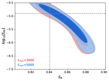
Regarding baryons, a common approach to protect analyses against their uncertain impact consists in excluding the deeply non-linear scales from the data vector (as in, e.g. Troxel et al., 2018; Amon et al., 2021), which in our case are the high-$\ell$ modes. Lowering the highest $\ell$ from 5000 to 3000 typically results in a degraded constraint on the modified gravity parameters, largely due to an increased degeneracy with $S_{8}$, but this degradation is not catastrophic, as shown in Fig. 13. This is consistent with our Fisher calculations, according to which the information partly saturates by $\ell=3000$. Therefore, while we expect the impact of varying $\ell_{\rm max}$ to lower the precision, the amount by which it does is not easily predictable due to the highly non-trivial degeneracies that exists in the high-dimensional likelihood space.

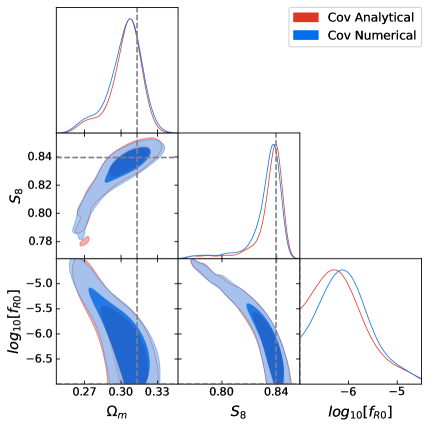
Finally, as mentioned earlier, an ingredient central to cosmological inference is the covariance matrix, which in the case of two-point statistics can be either modelled analytically or estimated numerically. This choice is not guaranteed to exists for all probes, and in fact many other weak lensing statistics must rely on an ensemble of mock data such as the SLICS to estimate the matrix. The validation process of these multi-purpose mocks generally includes a comparison with the analytical predictions for covariance matrix about two-point statistics. A first step of this comparison is shown already in Fig. 2, which visually demonstrate that the cross-correlation coefficient matrices are consistent with one another. A full quantitative validation must go beyond this, and we show in Fig. 14 the cosmological inference resulting from using the two matrices. We observe that both posteriors fully overlap, providing identical best-fit values on $\Omega_{\rm m}$, and differences on $S_{8}$ that vary by less than $0.3\sigma$. The upper limits of log${}_{10}\left[f_{R_{0}}\right]$ shift by under 1%, from $-5.08$ to $-5.05$. Note that the differences observed here are not exclusively caused by inaccuracies in the mocks, as many other factors can source important deviations, such as choices in the implementation of shape noise or masking (Joachimi et al., 2021b). In particular, the total survey areas match in both cases, however the analytical calculations assume a spherical survey whereas the mocks are square-shaped. Thus the small observed shifts in the cosmological inferences should be viewed as systematic uncertainties, not as biases, which thereby establishes the precision on the covariance one can expect from these SLICS mocks for any alternative weak lensing probes.

Also note that in an actual data analysis, the accuracy of the $B_{\delta}(k,z)$ emulator itself should be propagated into the covariance matrix in order to capture the modelling uncertainty.

Figure 14: Comparison between the cosmological inference resulting from using the analytical or the numerical covariance matrix when analysing the GR-$\Lambda$CDM simulated data.

5 Discussions and Conclusions

This paper introduces the MGLenS simulations, a large set of lensing maps sampling five cosmological and MG parameters within a volume that is wide and dense enough to analyse current Stage-III cosmic shear surveys. We demonstrate that the lensing power spectra measured from these simulations match well with the theoretical predictions obtained by the bridge and forge emulators, both at the level of the data vector and in a series of full gravito-cosmological inference analyses based on two-point statistics. Our results are robust to systematics such as multipole scale cuts, photometric redshift errors and intrinsic alignments of galaxies. We test our inference framework on theoretical data vectors using either an analytical or simulation-based covariance matrix, finding an excellent recovery of the input data vector.

Notably, we find that next generation lensing surveys will be powerful at constraining the gravity sector: in our simplified systematics-free analysis, we forecast that 5000 deg² of upcoming data could lead to $3\sigma$ detection of a value of $f_{R_{0}}$ as weak as $3.2\times 10^{-6}$, and $H_{0}r_{c}$ as low as 1.0. For weaker MG models, we find we are able to place an upper limit of $2.0\times 10^{-7}$ on $f_{R_{0}}$, and a lower limit of $2.6$ on $H_{0}r_{c}$, both at 95% CL. We acknowledge a number of caveats, including the absence of marginalisation over baryon feedback, or fixing the values of other cosmological parameters that have a secondary impact on the cosmic shear signal. These will inevitably translate into a slightly larger uncertainty budget in an more complete data analysis, however the statistical power displayed in our survey should remain relatively unchanged. Moreover, these forecasts are for auto-tomographic lensing data alone; adding cross-redshift bins, clustering and galaxy-galaxy lensing data could improve the constraints further. Another gain of precision could be achieved by analysing the data with non-Gaussian statistics.

When inferring cosmology from different input model vectors, we identify in many cases a strong degeneracy between the input $S_{8}$ value (related to the primordial power spectrum amplitude $A_{\rm s}$) and the modified gravity parameters; we propose new composite parameters that are better measured by lensing, namely $\zeta_{R_{0}}^{\alpha}$ and $\zeta_{r_{c}}^{\alpha}$, on which the precision is increased by up to a factor of two.

We lastly explored the impact of analysing data with the wrong gravity model, typically finding a catastrophic impact on the inferred cosmology with biases exceeding at times 20$\sigma$ in some cases, as well as an unphysical detection of MG features. The goodness-of-fit is generally best when using the correct gravity models, but some data are well fitted by GR, $f(R)$ and nDGP. This means that other analysis methods will need to be developed in order to better differentiate the gravity sector, such as Bayesian evidence ratios, the Suspiciousness metric, the recent empirical approach of Campos et al. (2022), or by looking at probes different from the lensing power spectrum.

The MGLenS simulations are organised as a series of flat-sky and curved-sky convergence maps, which can be analysed with any weak lensing statistics. Combined with the large SLICS ensemble produced for the evaluation of covariance matrix, the MGLenS suite are ideally suited to explore the sensitivity of novel statistics to cosmological and gravitational parameters, and can be used directly to analyse current Stage-III lensing surveys.

Data Availability

The MGLenS numerical simulations, the $B_{\delta}(k,z)$ CNN emulators and the cosmoSIS interface module will be made available upon acceptance to the Journal, while the SLICS simulations are already public.

Appendix A Curved-sky weak lensing light-cones

Table 5: Cosmological and gravity parameters of the forge and bridge simulations. The listed values of the structure growth parameters $\sigma_{8}$ and $S_{8}$ correspond to the input truth in the corresponding GR+$\Lambda$CDM simulations; the actual values in MGLenS are larger than these. Note that the emulators are specifically trained on $\Omega_{\rm m}$, $S_{8}$, $h$ and either log${}_{10}\left[f_{R_{0}}\right]$ or log${}_{10}\left[H_{0}r_{c}\right]$. In this paper we focus on weak, medium and strong models, which are respectively models-04, -18 and -13.

model	$\Omega_{\rm m}$	$\sigma_{8}$	$S_{8}$	$h$	$f_{R_{0}}$	$H_{0}r_{c}$
00	0.31315	0.82172	0.83954	0.6737	0	Inf
01	0.54725	0.49342	0.66642	0.78699	3.5502e-06	0.72533
02	0.53961	0.63783	0.85542	0.68393	3.0776e-06	0.81161
03	0.10721	1.2297	0.73513	0.6109	3.3107e-06	0.76647
04	0.31592	0.60111	0.61685	0.68845	8.0706e-07	3.9962
05	0.15741	0.91175	0.66044	0.71067	1.2093e-05	0.37375
06	0.35339	0.71886	0.78021	0.78052	5.2037e-06	0.56467
07	0.1124	1.2341	0.75539	0.79318	3.1185e-05	0.25000
08	0.39303	0.72152	0.82585	0.752	7.1372e-07	6.7113
09	0.18096	1.0378	0.80599	0.76132	9.1585e-07	3.3057
10	0.42927	0.5035	0.60228	0.77667	4.5479e-06	0.62132
11	0.40249	0.55523	0.64312	0.6912	1.3401e-06	1.7208
12	0.21286	1.0669	0.89867	0.70661	7.1154e-06	0.47331
13	0.34671	0.78191	0.84059	0.70056	1.2573e-05	0.36029
14	0.15464	0.9339	0.6705	0.77273	4.0961e-06	0.65314
15	0.28172	0.71367	0.69158	0.64968	4.9744e-06	0.59191
16	0.37032	0.61264	0.68066	0.76204	2.7753e-06	0.86134
17	0.41627	0.74242	0.87454	0.63427	1.4375e-05	0.33547
18	0.32331	0.85987	0.89266	0.81749	3.6751e-06	0.6877
19	0.47784	0.56403	0.71183	0.66724	6.7404e-06	0.49385
20	0.20509	0.75641	0.62541	0.64437	5.8109e-06	0.53938
21	0.44103	0.50237	0.60912	0.62046	6.2281e-06	0.51583
22	0.46403	0.5862	0.72906	0.80296	1.4121e-06	1.5615
23	0.13644	1.2584	0.84862	0.62473	1.0481e-06	2.4364
24	0.18832	0.85396	0.67659	0.80174	1.668e-05	0.32401
25	0.12066	1.3159	0.83454	0.69563	2.4559e-06	0.91639
26	0.28854	0.65331	0.6407	0.73943	8.7041e-06	0.43601
27	0.45016	0.72241	0.88492	0.71954	2.174e-05	0.2835
28	0.17155	1.1394	0.86159	0.62768	1.5757e-06	1.4266
29	0.51949	0.59577	0.78399	0.74473	9.6963e-06	0.40305
30	0.43909	0.61327	0.74195	0.67856	1.7774e-06	1.3111
31	0.49786	0.58288	0.75088	0.80806	1.8337e-06	1.2109
32	0.40909	0.54179	0.63268	0.73799	1.211e-06	1.9119
33	0.23227	0.86433	0.76052	0.60028	1.9037e-05	0.30276
34	0.3839	0.61174	0.69201	0.6557	2.2527e-06	1.0462
35	0.26234	0.88665	0.82914	0.76998	1.0089e-06	2.8097
36	0.25453	0.76212	0.702	0.66918	1.7789e-05	0.31312
37	0.29762	0.79347	0.79031	0.673	2.3584e-06	0.97764
38	0.22423	0.88911	0.76866	0.64603	1.3881e-05	0.34755
39	0.30799	0.71046	0.71985	0.66001	1.1732e-06	2.1452
40	0.51288	0.61834	0.80849	0.79098	7.8299e-06	0.45407
41	0.14061	1.1712	0.80186	0.73101	1.0743e-05	0.38798
42	0.33782	0.66702	0.70781	0.72256	7.9806e-07	5.0232
43	0.5252	0.66452	0.87924	0.81347	2.3279e-05	0.27454
44	0.19435	1.0172	0.8187	0.63911	2.7347e-05	0.25781
45	0.26963	0.91366	0.86618	0.75511	9.4886e-06	0.41903
46	0.49135	0.50927	0.65176	0.60766	2.5865e-05	0.26599
47	0.47207	0.58056	0.72827	0.61562	2.0816e-06	1.1234
48	0.24424	0.85676	0.77304	0.71436	6.6853e-07	10.0000
49	0.36187	0.56321	0.61856	0.72861	2.0258e-05	0.2929

Figure 15: Comparison between the curved- and flat-sky lensing power spectra. Plotted is the ratio between the measurements from the nodes 49 and 00, for all five tomographic redshift bins. The right-most plot exhibits large-scales systematics due to masking, which are increasingly important towards higher redshifts. Our flat-sky methods are mostly immune to this.

We develop a curved-sky ray-tracing algorithm adapted from UFalcon (Zürcher et al., 2021), in which the particle data falling into spherical mass shells are assigned onto a HealPIX (Górski et al., 2005) maps with nside=4096, instead of the Cartesian grids used in this paper. We again use periodic boundary conditions to fill the light-cone volume whenever it exits the simulation box, and repeat the procedure for 24 different observer’s positions. We modified the original UFalcon full-sky map making algorithm to implement instead a pencil-beam method, significantly reducing the memory load required to fill the high-redshift shells. This is achieved by stacking the simulation boxes along the [RA-Dec] = [0,0] direction only, and masking any pixel with RA/Dec $>$ 12 deg. Pseudo-independent light-cones are then extracted by selecting at random one of the 24 shells for each redshift, repeating the procedure 24 times per $N$-body simulation. The curved-sky angular power spectrum measurements are obtained from the standard Healpy routine map2alm, which performs Legendre transforms on the sphere and provides measurements for $\ell\in[1-12288]$, which we rebin to match the flat-sky measurements for an improved comparison.

We show that both flat- and curved-sky lensing simulations produce similar $C_{\ell}^{\kappa}$ measurements. Figure 15 presents the ratio between the lensing spectra from two models (the $f(R)$ model-49 and the GR model-00). The thin black lines present the mean over all flat-sky measurements while the thin blue lines show the curved-sky equivalent. The agreement between these two methods is excellent in the first four tomographic bins, whereas the last tomographic bin exhibits strong discrepancies on large scales. This is caused by the mixing between the maps and the mask, and can be removed with pseudo-$C_{\ell}$ estimators such as NaMaster (Alonso et al., 2019).

References

- Abbott et al. (2019) Abbott, T. M. C. et al. 2019, Phys. Rev. D, 99, 123505, 1810.02499
- Alonso et al. (2019) Alonso, D., Sanchez, J., Slosar, A., & LSST Dark Energy Science Collaboration. 2019, MNRAS, 484, 4127, 1809.09603
- Amon et al. (2021) Amon, A. et al. 2021, arXiv e-prints, arXiv:2105.13543, 2105.13543
- Angulo et al. (2021) Angulo, R. E., Zennaro, M., Contreras, S., Aricò, G., Pellejero-Ibañez, M., & Stücker, J. 2021, MNRAS, 507, 5869, 2004.06245
- Armijo et al. (2018) Armijo, J., Cai, Y.-C., Padilla, N., Li, B., & Peacock, J. A. 2018, MNRAS, 478, 3627, 1801.08975
- Arnold et al. (2019) Arnold, C., Leo, M., & Li, B. 2019, Nature Astron., 3, 945, 1907.02977
- Arnold et al. (2022) Arnold, C., Li, B., Giblin, B., Harnois-Déraps, J., & Cai, Y.-C. 2022, MNRAS, 515, 4161, 2109.04984
- Asgari et al. (2021) Asgari, M. et al. 2021, A&A, 645, A104, 2007.15633
- Babichev & Deffayet (2013) Babichev, E., & Deffayet, C. 2013, Class. Quant. Grav., 30, 184001, 1304.7240
- Babichev et al. (2009) Babichev, E., Deffayet, C., & Ziour, R. 2009, International Journal of Modern Physics D, 18, 2147, 0905.2943
- Barreira et al. (2015) Barreira, A., Bose, S., & Li, B. 2015, JCAP, 12, 059, 1511.08200
- Barreira et al. (2017) Barreira, A., Bose, S., Li, B., & Llinares, C. 2017, JCAP, 2017, 031, 1605.08436
- Barrera-Hinojosa et al. (2021) Barrera-Hinojosa, C., Li, B., Bruni, M., & He, J.-h. 2021, Mon. Not. Roy. Astron. Soc., 501, 5697, 2010.08257
- Blazek et al. (2019) Blazek, J. A., MacCrann, N., Troxel, M. A., & Fang, X. 2019, Phys. Rev. D, 100, 103506, 1708.09247
- Bose et al. (2015) Bose, S., Hellwing, W. A., & Li, B. 2015, JCAP, 02, 034, 1411.6128
- Bose et al. (2017) Bose, S., Li, B., Barreira, A., He, J.-h., Hellwing, W. A., Koyama, K., Llinares, C., & Zhao, G.-B. 2017, JCAP, 02, 050, 1611.09375
- Brax et al. (2004) Brax, P., van de Bruck, C., Davis, A. C., Khoury, J., & Weltman, A. 2004, AIP Conf. Proc., 736, 105, astro-ph/0410103
- Brax et al. (2008) Brax, P., van de Bruck, C., Davis, A.-C., & Shaw, D. J. 2008, Phys. Rev. D, 78, 104021, 0806.3415
- Bridle & King (2007) Bridle, S., & King, L. 2007, New Journal of Physics, 9, 444, 0705.0166
- Campos et al. (2022) Campos, A., Samuroff, S., & Mandelbaum, R. 2022, arXiv e-prints, arXiv:2211.02800, 2211.02800
- Casas et al. (2017) Casas, S., Kunz, M., Martinelli, M., & Pettorino, V. 2017, Physics of the Dark Universe, 18, 73, 1703.01271
- Charmousis et al. (2006) Charmousis, C., Gregory, R., Kaloper, N., & Padilla, A. 2006, JHEP, 10, 066, hep-th/0604086
- Chisari et al. (2018) Chisari, N. E. et al. 2018, MNRAS, 480, 3962, 1801.08559
- Crocce et al. (2006) Crocce, M., Pueblas, S., & Scoccimarro, R. 2006, MNRAS, 373, 369, astro-ph/0606505
- Cuesta-Lazaro et al. (2022) Cuesta-Lazaro, C., Arnold, C., Hernandez-Aguayo, C., Li, B., Giblin, B., Harnois-Déraps, J., & Cai, Y.-C. 2022, in prep.
- Davies et al. (2019) Davies, C. T., Cautun, M., & Li, B. 2019, MNRAS, 490, 4907, 1907.06657
- DES Collaboration et al. (2022) DES Collaboration et al. 2022, arXiv e-prints, arXiv:2207.05766, 2207.05766
- Dvali et al. (2000) Dvali, G. R., Gabadadze, G., & Porrati, M. 2000, Phys. Lett., B485, 208, hep-th/0005016
- Euclid Collaboration: Knabenhans et al. (2019) Euclid Collaboration: Knabenhans, M. et al. 2019, MNRAS, 484, 5509, 1809.04695
- Fairbairn & Goobar (2006) Fairbairn, M., & Goobar, A. 2006, Phys. Lett. B, 642, 432, astro-ph/0511029
- Fang et al. (2008) Fang, W., Wang, S., Hu, W., Haiman, Z., Hui, L., & May, M. 2008, Phys. Rev. D, 78, 103509, 0808.2208
- Feroz et al. (2009) Feroz, F., Hobson, M. P., & Bridges, M. 2009, MNRAS, 398, 1601, 0809.3437
- Giblin et al. (2021) Giblin, B. et al. 2021, A&A, 645, A105, 2007.01845
- Giocoli et al. (2018) Giocoli, C., Baldi, M., & Moscardini, L. 2018, MNRAS, 481, 2813, 1806.04681
- Górski et al. (2005) Górski, K. M., Hivon, E., Banday, A. J., Wandelt, B. D., Hansen, F. K., Reinecke, M., & Bartelmann, M. 2005, ApJ, 622, 759, astro-ph/0409513
- Hamana et al. (2020) Hamana, T. et al. 2020, PASJ, 72, 16, 1906.06041
- Harnois-Déraps et al. (2019) Harnois-Déraps, J., Giblin, B., & Joachimi, B. 2019, A&A, 631, A160, 1905.06454
- Harnois-Déraps et al. (2022) Harnois-Déraps, J., Martinet, N., & Reischke, R. 2022, MNRAS, 509, 3868, 2107.08041
- Harnois-Déraps et al. (2015) Harnois-Déraps, J., Munshi, D., Valageas, P., van Waerbeke, L., Brax, P., Coles, P., & Rizzo, L. 2015, MNRAS, 454, 2722, 1506.06313
- Harnois-Déraps & van Waerbeke (2015) Harnois-Déraps, J., & van Waerbeke, L. 2015, MNRAS, 450, 2857, 1406.0543
- Harnois-Déraps et al. (2015) Harnois-Déraps, J., van Waerbeke, L., Viola, M., & Heymans, C. 2015, MNRAS, 450, 1212
- Heitmann et al. (2014) Heitmann, K., Lawrence, E., Kwan, J., Habib, S., & Higdon, D. 2014, ApJ, 780, 111, 1304.7849
- Hendrycks & Gimpel (2016) Hendrycks, D., & Gimpel, K. 2016, arXiv e-prints, arXiv:1606.08415, 1606.08415
- Hernández-Aguayo et al. (2021) Hernández-Aguayo, C., Arnold, C., Li, B., & Baugh, C. M. 2021, Mon. Not. Roy. Astron. Soc., 503, 3867, 2006.15467
- Hernández-Aguayo et al. (2018) Hernández-Aguayo, C., Baugh, C. M., & Li, B. 2018, Mon. Not. Roy. Astron. Soc., 479, 4824, 1801.08880
- Hernández-Aguayo et al. (2022) Hernández-Aguayo, C., Ruan, C.-Z., Li, B., Arnold, C., Baugh, C. M., Klypin, A., & Prada, F. 2022, JCAP, 2022, 048, 2110.00566
- Heydenreich et al. (2022) Heydenreich, S., Brück, B., Burger, P., Harnois-Déraps, J., Unruh, S., Castro, T., Dolag, K., & Martinet, N. 2022, arXiv e-prints, arXiv:2204.11831, 2204.11831
- Heymans et al. (2021) Heymans, C. et al. 2021, A&A, 646, A140, 2007.15632
- Higuchi & Shirasaki (2016) Higuchi, Y., & Shirasaki, M. 2016, MNRAS, 459, 2762, 1603.01325
- Hikage et al. (2019) Hikage, C. et al. 2019, PASJ, 71, 43, 1809.09148
- Hildebrandt et al. (2021) Hildebrandt, H. et al. 2021, A&A, 647, A124, 2007.15635
- Hinterbichler & Khoury (2010) Hinterbichler, K., & Khoury, J. 2010, Phys. Rev. Lett., 104, 231301, 1001.4525
- Hinterbichler et al. (2011) Hinterbichler, K., Khoury, J., Levy, A., & Matas, A. 2011, Phys. Rev. D, 84, 103521, 1107.2112
- Hirata & Seljak (2004) Hirata, C. M., & Seljak, U. 2004, Phys. Rev. D, 70, 063526, astro-ph/0406275
- Hobson et al. (2002) Hobson, M. P., Bridle, S. L., & Lahav, O. 2002, MNRAS, 335, 377, astro-ph/0203259
- Hojjati et al. (2011) Hojjati, A., Zhao, G. B., Pogosian, L., & Silvestri, A. 2011, MGCAMB: Modification of Growth with CAMB, Astrophysics Source Code Library, record ascl:1106.013, 1106.013
- Hu & Sawicki (2007) Hu, W., & Sawicki, I. 2007, Phys. Rev., D76, 064004, 0705.1158
- Joachimi et al. (2021a) Joachimi, B., Köhlinger, F., Handley, W., & Lemos, P. 2021a, A&A, 647, L5, 2102.09547
- Joachimi et al. (2021b) Joachimi, B. et al. 2021b, A&A, 646, A129, 2007.01844
- Joudaki et al. (2017) Joudaki, S. et al. 2017, MNRAS, 471, 1259, 1610.04606
- Khoury & Weltman (2004a) Khoury, J., & Weltman, A. 2004a, Phys. Rev. D, 69, 044026, astro-ph/0309411
- Khoury & Weltman (2004b) ——. 2004b, Phys. Rev. Lett., 93, 171104, astro-ph/0309300
- Kilbinger et al. (2017) Kilbinger, M. et al. 2017, MNRAS, 472, 2126, 1702.05301
- Kingma & Ba (2014) Kingma, D. P., & Ba, J. 2014, arXiv e-prints, arXiv:1412.6980, 1412.6980
- Koyama (2016) Koyama, K. 2016, Reports on Progress in Physics, 79, 046902, 1504.04623
- Koyama & Silva (2007) Koyama, K., & Silva, F. P. 2007, Phys. Rev. D, 75, 084040, hep-th/0702169
- Lemos et al. (2020) Lemos, P., Köhlinger, F., Handley, W., Joachimi, B., Whiteway, L., & Lahav, O. 2020, MNRAS, 496, 4647, 1910.07820
- Lemos et al. (2022) Lemos, P. et al. 2022, arXiv e-prints, arXiv:2202.08233, 2202.08233
- Lewis et al. (2000) Lewis, A., Challinor, A., & Lasenby, A. 2000, Astrophys. J., 538, 473, astro-ph/9911177
- Li (2018) Li, B. 2018, Simulating Large-Scale Structure for Models of Cosmic Acceleration, 2514-3433 (IOP Publishing)
- Li et al. (2013a) Li, B., Barreira, A., Baugh, C. M., Hellwing, W. A., Koyama, K., Pascoli, S., & Zhao, G.-B. 2013a, JCAP, 11, 012, 1308.3491
- Li & Shirasaki (2018) Li, B., & Shirasaki, M. 2018, MNRAS, 474, 3599, 1710.07291
- Li et al. (2013b) Li, B., Zhao, G.-B., & Koyama, K. 2013b, JCAP, 05, 023, 1303.0008
- Li et al. (2012) Li, B., Zhao, G.-B., Teyssier, R., & Koyama, K. 2012, JCAP, 2012, 051, 1110.1379
- Llinares (2018) Llinares, C. 2018, Int. J. Mod. Phys. D, 27, 1848003, 2103.10890
- Lombriser et al. (2009) Lombriser, L., Hu, W., Fang, W., & Seljak, U. 2009, Phys. Rev. D, 80, 063536, 0905.1112
- Luty et al. (2003) Luty, M. A., Porrati, M., & Rattazzi, R. 2003, JHEP, 09, 029, hep-th/0303116
- Maartens & Majerotto (2006) Maartens, R., & Majerotto, E. 2006, Phys. Rev. D, 74, 023004, astro-ph/0603353
- Marshall et al. (2006) Marshall, P., Rajguru, N., & Slosar, A. 2006, Phys. Rev. D, 73, 067302, astro-ph/0412535
- Martinelli et al. (2011) Martinelli, M., Calabrese, E., de Bernardis, F., Melchiorri, A., Pagano, L., & Scaramella, R. 2011, Phys. Rev. D, 83, 023012, 1010.5755
- Martinet et al. (2021a) Martinet, N., Castro, T., Harnois-Déraps, J., Jullo, E., Giocoli, C., & Dolag, K. 2021a, A&A, 648, A115, 2012.09614
- Martinet et al. (2021b) Martinet, N., Harnois-Déraps, J., Jullo, E., & Schneider, P. 2021b, A&A, 646, A62, 2010.07376
- Mead et al. (2021) Mead, A. J., Brieden, S., Tröster, T., & Heymans, C. 2021, MNRAS, 502, 1401, 2009.01858
- Mota & Shaw (2006) Mota, D. F., & Shaw, D. J. 2006, Phys. Rev. Lett., 97, 151102, hep-ph/0606204
- Oyaizu (2008) Oyaizu, H. 2008, Phys. Rev. D, 78, 123523, 0807.2449
- Peel et al. (2018) Peel, A., Pettorino, V., Giocoli, C., Starck, J.-L., & Baldi, M. 2018, A&A, 619, A38, 1805.05146
- Petri (2016) Petri, A. 2016, Astronomy and Computing, 17, 73
- Pratten et al. (2016) Pratten, G., Munshi, D., Valageas, P., & Brax, P. 2016, Phys. Rev. D, 93, 103524, 1602.06711
- Ruan et al. (2022) Ruan, C.-Z., Hernández-Aguayo, C., Li, B., Arnold, C., Baugh, C. M., Klypin, A., & Prada, F. 2022, JCAP, 05, 018, 2110.00328
- Schmidt (2008) Schmidt, F. 2008, Phys. Rev. D, 78, 043002, 0805.4812
- Schmidt (2009) ——. 2009, Phys. Rev. D, 80, 123003, 0910.0235
- Secco et al. (2021) Secco, L. F. et al. 2021, arXiv e-prints, arXiv:2105.13544, 2105.13544
- Semboloni et al. (2011) Semboloni, E., Hoekstra, H., Schaye, J., van Daalen, M. P., & McCarthy, I. G. 2011, MNRAS, 1461
- Shirasaki et al. (2017) Shirasaki, M., Nishimichi, T., Li, B., & Higuchi, Y. 2017, MNRAS, 466, 2402, 1610.03600
- Springel (2010) Springel, V. 2010, MNRAS, 401, 791, 0901.4107
- Springel et al. (2005) Springel, V. et al. 2005, Nature, 435, 629, astro-ph/0504097
- Takada & Jain (2009) Takada, M., & Jain, B. 2009, MNRAS, 395, 2065
- Takahashi et al. (2012) Takahashi, R., Sato, M., Nishimichi, T., Taruya, A., & Oguri, M. 2012, ApJ, 761, 152
- Thomas et al. (2009) Thomas, S. A., Abdalla, F. B., & Weller, J. 2009, MNRAS, 395, 197, 0810.4863
- Tröster et al. (2021) Tröster, T. et al. 2021, A&A, 649, A88, 2010.16416
- Troxel et al. (2018) Troxel, M. A. et al. 2018, Phys. Rev. D, 98, 043528, 1708.01538
- Vainshtein (1972) Vainshtein, A. I. 1972, Physics Letters B, 39, 393
- Valogiannis & Bean (2017) Valogiannis, G., & Bean, R. 2017, Phys. Rev. D, 95, 103515, 1612.06469
- van den Busch et al. (2022) van den Busch, J. L. et al. 2022, A&A, 664, A170, 2204.02396
- Weinberger et al. (2020) Weinberger, R., Springel, V., & Pakmor, R. 2020, ApJS, 248, 32, 1909.04667
- Will (2006) Will, C. M. 2006, Living Rev. Rel., 9, 3, gr-qc/0510072
- Will (2014) ——. 2014, Living Rev. Rel., 17, 4, 1403.7377
- Winther et al. (2015) Winther, H. A., et al. 2015, Mon. Not. Roy. Astron. Soc., 454, 4208, 1506.06384
- Wright et al. (2020) Wright, A. H., Hildebrandt, H., van den Busch, J. L., Heymans, C., Joachimi, B., Kannawadi, A., & Kuijken, K. 2020, A&A, 640, L14, 2005.04207
- Zorrilla Matilla et al. (2020) Zorrilla Matilla, J. M., Waterval, S., & Haiman, Z. 2020, AJ, 159, 284, 1909.12345
- Zuntz et al. (2015) Zuntz, J. et al. 2015, Astronomy and Computing, 12, 45
- Zürcher et al. (2021) Zürcher, D., Fluri, J., Sgier, R., Kacprzak, T., & Refregier, A. 2021, JCAP, 2021, 028, 2006.12506