Sketched Gaussian Model Linear Discriminant Analysis via the Randomized Kaczmarz Method

Abstract

We present sketched linear discriminant analysis, an iterative randomized approach to binary-class Gaussian model linear discriminant analysis (LDA) for very large data. We harness a least squares formulation and mobilize the stochastic gradient descent framework. Therefore, we obtain a randomized classifier with performance that is very comparable to that of full data LDA while requiring access to only one row of the training data at a time. We present convergence guarantees for the sketched predictions on new data within a fixed number of iterations. These guarantees account for both the Gaussian modeling assumptions on the data and algorithmic randomness from the sketching procedure. Finally, we demonstrate performance with varying step-sizes and numbers of iterations. Our numerical experiments demonstrate that sketched LDA can offer a very viable alternative to full data LDA when the data may be too large for full data analysis.

Keywords: classification, stochastic optimization, supervised learning

1 Introduction

Linear discriminant analysis (LDA) is a classic method of supervised learning, or classification. Its many applications include classification in genetics [79, 77], facial recognition [44, 43], pattern recognition [16], hyperspectral imaging [24], and chemometrics [32] to name a few. Consider a matrix $\mathbf{X}\in\mathbb{R}^{n\times p}$, where each row contains an observation with measurements on $p$ variables, or features. Each observation $\mathbf{x}\in\mathbb{R}^{p}$ belongs to one of two classes with class label $y$ so that $y=1$ for Group 1 and $y=0$ for Group 2. Gaussian model LDA assumes that the class-conditional distribution for each observation $p(\mathbf{x}\;|\;y)$ is multivariate Gaussian with class means $\bm{\mu}_{1}\in\mathbb{R}^{p}$ and $\bm{\mu}_{2}$ $\in\mathbb{R}^{p}$ for Groups 1 and 2, respectively, and common covariance $\mathbf{\Sigma}\in\mathbb{R}^{p\times p}$. Therefore, we can employ Bayes rule to identify a linear decision boundary for classifying observations to the most likely class.

For moderately sized data in the overdetermined case where $n>p$, Gaussian model LDA is a classic statistical method of supervised learning. However, it encounters limitations when either $n$, or both $n$ and $p$, are very large. If $n$ is very large, it may be infeasible to store the entire dataset in working memory on a local machine. If $p$ is very large, it may be very costly to perform an eigenvalue decomposition on the covariance matrix $\mathbf{\Sigma}$ to obtain the LDA classification direction.

We harness the least squares formulation of LDA for the binary-class Gaussian model and propose sketched LDA for binary-class Gaussian classification via the randomized Kaczmarz method [72, 45, 46, 52, 53, 17, 12, 42, 59, 1, 58, 71, 83]. The randomized Kaczmarz method is an instance of stochastic gradient descent (SGD) [68] applied to least squares problems with a specific step-size that depends on the row chosen in a given iteration [53]. SGD is a well-known randomized approach to handling very large data problems [6, 7, 55]. By employing a least squares formulation, we can mobilize the SGD framework to obtain a sketched LDA classifier with performance that is very comparable to that of full data Gaussian model LDA while requiring access to only one row of the training data at a time. The keys to our method and analysis lie in combining the following facts.

1. For two classes, the full data least squares formulation of LDA produces the same direction as Gaussian model LDA ([34, Section 4.3, Exercise 4.2], [67, Section 3.2]).

2. The randomized Kaczmarz method is a special case of SGD with importance sampling applied to least squares problems. Moreover, the randomized Kaczmarz method with importance sampling converges exponentially to a horizon, or within a radius, of the least squares solution [72, 52, 53]. Therefore, the randomized Kaczmarz method solution of the least squares formulation of LDA converges to a horizon of the binary-class Gaussian model LDA direction.

3. Convergence guarantees for the randomized Kaczmarz method account for randomness from the iterates [53, 52, 31, 40]. However, one can account for both the Gaussian modeling assumptions in the data and algorithmic randomness from the randomized Kaczmarz iterates by applying the Law of Total Expectations [15, 47]. Therefore, we obtain convergence guarantees for the sketched LDA predictions on new data that account for both the randomness from the modeling assumptions and algorithmic randomness due to the sketching procedure.

Our theoretical results in Section 3 present convergence guarantees for the sketched LDA predictions on new data with a finite number of iterations and importance sampling. Our numerical experiments in Section 4 demonstrate that sketched LDA can offer a very viable alternative to binary class full data Gaussian model LDA when the data may be too large for full data analysis.

1.1 Related works

The least squares formulation of binary-class LDA is well-known ([34, Section 4.3, Exercise 4.2], [67, Section 3.2]) and has been employed for binary-class sparse discriminant analysis in ultrahigh dimensions [49]. For more than two classes, a least squares formulation is also available for Fisher’s LDA [29, 81], which does not require distributional assumptions on the data and is not the same as Gaussian model LDA in general. The least squares formulation has also been employed in other versions of discriminant analysis, including discriminant analysis by optimal scaling [9] and flexible discriminant analysis [34, Section 12.5]. These methods allow for potentially non-linear transformations of the class labels.

In recent years, sketching – or dimension reduction by random sampling, random projections, or a combination of both – has become a popular approach to large data problems. Sketching as a subspace embedding is commonly thought to have first appeared in [70]. Common classifications depend on whether the sketch achieves row compression [8, 22, 23, 37, 15, 14, 47, 64, 69], column compression [4, 38, 50, 74, 82], or both [51].

Some stochastic optimization algorithms can be viewed as variations on sketching [31]. One example is the randomized Kaczmarz method (RK) [72, 45, 46, 52, 53, 17, 12, 42, 59, 1, 58, 71, 83, 39]. Given $\mathbf{A}\in\mathbb{R}^{n\times p}$ and $\mathbf{b}\in\mathbb{R}^{n}$, the Kaczmarz method is an iterative algorithm for computing solutions to linear systems of the form $\mathbf{A}\mathbf{x}=\mathbf{b}$ [39]. While the Kaczmarz method proceeds through the rows of $\mathbf{A}$, the RK randomly samples a row from $\mathbf{A}$ in the $k^{th}$ iteration and projects the $k^{th}$ update onto the subspace spanned by the regression residual from the $k^{th}$ row. Therefore, the RK is an example of a sketch-and-project approach [31, 30] since random sampling from the rows of a matrix can be expressed as left multiplication with a sketching matrix. Strohmer and Vershynin showed in [72] that the RK converges exponentially in expectation if the rows are selected with probabilities proportional to their row norms. Variations on the RK now include applications to inconsistent linear systems [52], optimal weighting probabilities [31], hybrid Kaczmarz approaches [19], and a block Gaussian Kaczmarz method [65]. Section 2.3 contains additional details on the RK.

Some works on sketched LDA and its variations exist. These focus on sketching via subspace embeddings and include random Gaussian projections of the feature vectors [25], fast Johnson-Lindenstrauss transform (FJLT) [2] projection for Fisher’s LDA [80], and random projections in LDA ensembles [26]. These utilize the well-known two-step sketched subspace procedure of first performing efficient dimension reduction with a suitable random sketching matrix, and then solving the problem directly in the reduced dimension.

However, this two-step random projections approach has limited applicability in analyzing massive data. Although applying a random projection requires less computation time than dense matrix-matrix multiplication when utilizing FJLTs, it still requires $\mathcal{O}(np\log p)+\text{poly}\left(\frac{p}{\epsilon}\right)$ time [78, page 7] when $n>p$ and $\epsilon$ is the desired error level. Thus, the computation time required will be extraordinarily large for massive data. As an alternative for very large data, we consider sketched LDA via the RK in this work.

2 Background

We begin with an overview of some background material to set the stage for our presentation of sketched LDA via the RK. We define notation, review Gaussian model LDA in Section 2.1, and examine the least squares approach to binary Gaussian model LDA in Section 2.2. We then introduce the RK in Section 2.3.

We assume that all vectors are column vectors. Given a matrix $\mathbf{X}$, we denote its $j^{th}$ row by $\mathbf{x}_{j}^{\sf T}$, its Frobenius norm by $\|\mathbf{X}\|_{F}$, and its operator norm by $\|\mathbf{X}\|_{2}$. We denote the following scaled condition number of $\mathbf{X}$ by $\kappa(\mathbf{X})=\|\mathbf{X}\|_{F}^{2}\|(\mathbf{X}^{\sf T}\mathbf{X})^{-1}\|_{2}$ or $\kappa(\mathbf{X})=\|\mathbf{X}\|_{F}^{2}\|(\mathbf{X}^{\sf T}\mathbf{X})^{\dagger}\|_{2}$ if $\mathbf{X}$ does not have full column rank. This is related to the square of the scaled condition number for square matrices in [20]. Given an integer $n$, we employ $[n]$ to denote the set $\{1,2,\dots,n\}$. We employ ${\bf 1}_{n}$ to denote the vector of length $n$ whose entries are all $1$. We utilize $\mathbf{e}_{j}$ to denote the canonical basis vector whose $j^{th}$ entry is $1$ and whose entries are $0$ everywhere else.

2.1 Gaussian Model LDA

We review the Gaussian model approach to LDA to underscore the computational difficulties arising from computing an LDA classifier for very large data where $n>p$, and $n$ and $p$ may both be very large. Let $\mathbf{y}\in\mathbb{R}^{n}$ be a vector containing the class labels for the $n$ observations, each belonging to one of $g$ classes. Additionally, let the feature vector and class label for the $i^{th}$ observation be denoted by $\mathbf{x}_{i}$ and $y_{i}$, respectively.

Gaussian model LDA assumes that observations follow class-conditional Gaussian distributions with class means $\bm{\mu}_{k}\in\mathbb{R}^{p}$ for $1\leq k\leq g$, common covariance $\mathbf{\Sigma}\in\mathbb{R}^{p\times p}$, and prior probability $\pi_{k}$ of belonging to the $k^{th}$ class with $\sum_{k=1}^{g}\pi_{k}=1$. Suppose that $\mathbf{\Sigma}$ is nonsingular. For any new observation $\mathbf{\tilde{x}}\in\mathbb{R}^{p}$, Bayes rule provides the following classification rule ([34, Section 4.3], [67, Section 3.1])

$$\tilde{y} = \arg\max_{k}\delta_{k}(\mathbf{\tilde{x}}),$$ (1)

where

$$\delta_{k}(\mathbf{\tilde{x}}) = \log\pi_{k}+\mathbf{\tilde{x}}^{\sf T}\mathbf{\Sigma}^{-1}\bm{\mu}_{k}-\frac{1}{2}\bm{\mu}_{k}^{\sf T}\mathbf{\Sigma}^{-1}\bm{\mu}_{k}\quad\text{for}\quad 1\leq k\leq g$$ (2)

are the linear discriminant functions.

Since $\pi_{k},{\bm{\mathbf{{\mu}}}}_{k},$ and $\mathbf{\Sigma}$ are typically unknown, we employ their data-dependent estimates. Let $n_{k}$ denote the number of observations in the $k^{th}$ class. Then we define

$$\hat{\pi}_{k} = \frac{n_{k}}{n},$$

$$\hat{\bm{\mu}}_{k} = \sum_{y_{i}=k}\frac{1}{n_{k}}\,\mathbf{x}_{i}\,,\quad\text{and}$$

$$\hat{\mathbf{\Sigma}} = \frac{1}{n-g}\sum_{k=1}^{g}\sum_{y_{i}=k}(\mathbf{x}_{i}-\hat{\bm{\mu}}_{k})(\mathbf{x}_{i}-\hat{\bm{\mu}}_{k})^{\sf T}.$$

In practice, we do not compute $\mathbf{\Sigma}^{-1}$ explicitly. Rather than maximizing (2), we can equivalently minimize

$$\delta_{k}^{*}(\mathbf{\tilde{x}}) = -\delta_{k}(\mathbf{\tilde{x}})+\frac{1}{2}\mathbf{\tilde{x}}^{\sf T}\mathbf{\Sigma}^{-1}\mathbf{\tilde{x}}$$ (3)

$$= \frac{1}{2}(\mathbf{\tilde{x}}-\bm{\mu}_{k})^{\sf T}\mathbf{\Sigma}^{-1}(\mathbf{\tilde{x}}-\bm{\mu}_{k})-\log\pi_{k},$$

since the additive term does not depend on $k$. We recognize the first term on the right in (3) as the squared Mahalanobis distance between the new observation $\mathbf{\tilde{x}}$ and the distribution of the $k^{th}$ class. Let $\mathbf{\Sigma}=\mathbf{V}\mathbf{D}\mathbf{V}^{\sf T}$ be an eigenvalue decomposition of $\mathbf{\Sigma}$. Since we assume that $\mathbf{\Sigma}$ is nonsingular, $\mathbf{\Sigma}^{-1}=\mathbf{V}\mathbf{D}^{-1}\mathbf{V}^{\sf T}$ and we rewrite the first term in (3) as

$$\frac{1}{2}(\mathbf{\tilde{x}}-\bm{\mu}_{k})^{\sf T}\mathbf{\Sigma}^{-1}(\mathbf{\tilde{x}}-\bm{\mu}_{k}) = \frac{1}{2}\|\mathbf{D}^{-\frac{1}{2}}\mathbf{V}^{\sf T}(\mathbf{\tilde{x}}-\bm{\mu}_{k})\|_{2}^{2}$$

$$= \frac{1}{2}\|\mathbf{x}^{*}-\bm{\mu}_{k}^{*}\|_{2}^{2},$$

where $\mathbf{x}^{*}=\mathbf{D}^{-\frac{1}{2}}\mathbf{V}^{\sf T}\mathbf{\tilde{x}}$ and $\bm{\mu}_{k}^{*}=\mathbf{D}^{-\frac{1}{2}}\mathbf{V}^{\sf T}\bm{\mu}_{k}$. Therefore, we rewrite (3) as

$$\delta_{k}^{*}(\mathbf{\tilde{x}}) = \frac{1}{2}\|\mathbf{\tilde{x}}^{*}-\bm{\mu}_{k}^{*}\|_{2}^{2}-\log\pi_{k}.$$ (4)

Applying $\mathbf{D}^{-\frac{1}{2}}\mathbf{V}^{\sf T}$ on the left in (4) has a sphering effect since the sphered data $\mathbf{D}^{-\frac{1}{2}}\mathbf{V}^{\sf T}\mathbf{X}$ have identity covariance. Therefore, classifying $\mathbf{\tilde{x}}^{*}$ to the group with smallest $\delta_{k}^{*}$ is equivalent to classifying to the nearest centroid after sphering the data and adjusting for class proportions. Algorithm 1 summarizes the procedures for computing the Gaussian model LDA classifier.

Algorithm 1 Gaussian Model LDA

Input: Labeled data $(\mathbf{y}\in\mathbb{R}^{n},\mathbf{X}\in\mathbb{R}^{n\times p})$ and new unlabeled observation $\mathbf{\tilde{x}}\in\mathbb{R}^{p}$
Output: Predicted class label $\tilde{y}$ for $\mathbf{\tilde{x}}$

1:  Compute estimates $\hat{\pi}_{k},\hat{\bm{\mu}}_{k}$ for $1\leq k\leq g$ and $\hat{\mathbf{\Sigma}}$:

2:  $\quad\hat{\pi}_{k}=\frac{n_{k}}{n}$

3:  $\quad\hat{\bm{\mu}}_{k}=\sum_{y_{i}=k}\frac{1}{n_{k}}\mathbf{x}_{i}$

4:  $\quad\hat{\mathbf{\Sigma}}=\frac{1}{n-g}\sum_{k=1}^{g}\sum_{y_{i}=k}(\mathbf{x}_{i}-\hat{\bm{\mu}}_{k})(\mathbf{x}_{i}-\hat{\bm{\mu}}_{k})^{\sf T}$

5:  $\hat{\mathbf{\Sigma}}=\mathbf{V}\mathbf{D}\mathbf{V}^{\sf T}$ // Compute eigenvalue decomposition for $\hat{\mathbf{\Sigma}}$

6:  $\bm{\mu}_{k}^{*}=\mathbf{D}^{-\frac{1}{2}}\mathbf{V}^{\sf T}\hat{\bm{\mu}}_{k}$  for  $1\leq k\leq g$ // Sphere centroids

7:  $\mathbf{\tilde{x}}^{*}=\mathbf{D}^{-\frac{1}{2}}\mathbf{V}^{\sf T}\mathbf{\tilde{x}}$  // Sphere unlabeled observation

8:  $\delta_{k}^{*}=\frac{1}{2}\|\mathbf{\tilde{x}}^{*}-\hat{\bm{\mu}}_{k}^{*}\|_{2}-\log\hat{\pi}_{k}$  for  $1\leq k\leq g$ // Compute discriminant functions for $\mathbf{\tilde{x}}^{*}$

9:  return  $\tilde{y}=\arg\min_{k}\delta_{k}^{*}(\mathbf{\tilde{x}}^{*})$ // Classify to class with least $\delta_{k}^{*}$

Algorithm 1 highlights how the computational burden in solving (1) is in forming $\hat{\mathbf{\Sigma}}$ and computing an eigenvalue (or singular value) decomposition for it. This is straightforward for moderately sized data but is computationally burdensome when $n$ is very large or both $n$ and $p$ are very large since forming $\hat{\mathbf{\Sigma}}$ requires $\mathcal{O}(np^{2})$ computations and computing its eigenvalue decomposition requires $\mathcal{O}(p^{3})$ computations [61].

2.2 Least Squares LDA

For binary classification problems, we can employ least squares regression to obtain a Gaussian model LDA classifier in lieu of Algorithm 1. Therefore, we focus on the fundamental LDA problem of binary classification in the overdetermined case with $n>p$, where (1) reduces to the following decision rule: we classify $\mathbf{\tilde{x}}$ to the second class if and only if

$$\delta_{\text{LDA}}=\left\{\mathbf{\tilde{x}}-\frac{1}{2}(\bm{\mu}_{1}+\bm{\mu}_{2})\right\}^{\sf T}\mathbf{\Sigma}^{-1}(\bm{\mu}_{2}-\bm{\mu}_{1})+\log\left(\frac{\pi_{2}}{\pi_{1}}\right)>0.$$ (5)

Let $\bm{\beta}^{\text{LDA}}=\mathbf{\Sigma}^{-1}(\bm{\mu}_{2}-\bm{\mu}_{1})$ denote the LDA classifier in (5). Then binary Gaussian model LDA can be cast as a least squares regression problem, where the least squares solution vector is proportional to $\bm{\beta}^{\text{LDA}}$ ([34, Section 4.3, Exercise 4.2], [67, Section 3.2]).

Following the approach in ([29, Section 4], [34, Exercise 4.2], [49, Section 3.1]), we recode the class labels as $y_{i}=-\frac{n}{n_{1}}$ for observations belonging to Class 1 or $y_{i}=\frac{n}{n_{2}}$ for Class 2 with $1\leq i\leq n$. We then obtain the Bayes LDA classifier direction by first solving

$$\begin{pmatrix}\hat{\beta}_{\text{o}}\\ \hat{\bm{\beta}}^{\text{LS}}\end{pmatrix}=\arg\min_{\beta_{\text{o}},\,\bm{\beta}}\left\{\frac{1}{2}\sum_{i=1}^{n}(y_{i}-\beta_{\text{o}}-\mathbf{x}_{i}^{\sf T}\bm{\beta})^{2}\right\}.$$ (6)

Let $\hat{\beta}_{\text{o}}^{\text{opt}}$ denote an optimal choice of the intercept $\hat{\beta}_{\text{o}}$. Then we classify $\mathbf{\tilde{x}}$ to the second class if and only if

$$\delta_{\text{LSLDA}}=\mathbf{\tilde{x}}^{\sf T}\hat{\bm{\beta}}^{\text{LS}}+\hat{\beta}_{\text{o}}^{\text{opt}}>0.$$ (7)

2.2.1 Computing the Intercept

The direction vector $\hat{\bm{\beta}}^{\text{LDA}}$ produced by Gaussian model LDA with Algorithm 1 does not give rise to an intercept term. To obtain a direction vector $\hat{\bm{\beta}}^{\text{LS}}$ with Algorithm 2 that is a scalar multiple of $\hat{\bm{\beta}}^{\text{LDA}}$ so that the LDA direction remains unchanged, however, requires fitting an intercept in the least squares model. We illustrate this in our numerical experiments in Section 4, where $\hat{\bm{\beta}}^{\text{LS}}$ estimated with the intercept term $\beta_{0}$ in (6) is a scalar multiple of $\hat{\bm{\beta}}^{\text{LDA}}$ so that the decision boundaries $\delta_{\text{LDA}}$ and $\delta_{\text{LSLDA}}$ from (5) and (7) coincide.

The choice of the intercept term affects the LDA classifier substantially, however, and there are multiple approaches to selecting it. For example, [34, Section 4.3] recommends selecting the intercept via a data-driven approach that minimizes the training error for a given dataset. Meanwhile, [49, Proposition 2] shows that the following closed-form expression for the intercept term is optimal in the sense that it minimizes the expected prediction error on new data

$$\hat{\beta}_{\text{o}}^{\text{opt}}=-\frac{1}{2}(\hat{\bm{\mu}}_{1}+\hat{\bm{\mu}}_{2})^{\sf T}\hat{\bm{\beta}}^{\text{LS}}+(\hat{\bm{\beta}}^{\text{LS}})^{\sf T}\hat{\mathbf{\Sigma}}\hat{\bm{\beta}}^{\text{LS}}\{(\hat{\bm{\mu}}_{2}-\hat{\bm{\mu}}_{1})^{\sf T}\hat{\bm{\beta}}^{\text{LS}}\}^{-1}\log\left(\frac{n_{2}}{n_{1}}\right).$$ (8)

If we assume that $\hat{\bm{\beta}}^{\text{LS}}=\eta\hat{\bm{\beta}}^{\text{LDA}}=\eta\mathbf{\Sigma}^{-1}(\bm{\mu}_{2}-\bm{\mu}_{1})$ for some $\eta\neq 0$ and employ this in the second term in (8), we obtain $\hat{\beta}_{\text{o}}^{\text{opt}}=\eta\hat{\beta}_{\text{o}}^{\text{LDA}},$ where we obtain $\hat{\beta}_{\text{o}}^{\text{LDA}}$ by solving for $\beta_{\text{o}}$ with (5) and (7) from the Gaussian model. This is reassuring since it yields $\delta_{\text{LSLDA}}=\eta\,\delta_{\text{LDA}}$ so that the decision boundary remains unchanged.

Since $\eta$ is unknown, we employ the optimal $\hat{\beta}_{\text{o}}^{\text{opt}}$ from (8) in our experiments in Section 4. Algorithm 2 summarizes the procedures for computing the binary Gaussian model LDA classifier via least squares regression. While the least squares approach to LDA omits Gaussian assumptions [34], determining an optimal intercept via (8) assumes class-conditional Gaussian observations. Additionally, (8) requires computing $\hat{\mathbf{\Sigma}}\in\mathbb{R}^{p\times p}$, which can be costly if $p$ is very large. One solution may involve approximations of $\hat{\mathbf{\Sigma}}$ in these cases. A sketch of the proof for $\hat{\beta}_{\text{o}}^{\text{opt}}$ is in [49]. The supplement contains the details.

Algorithm 2 Binary Class Gaussian Model LDA via Least Squares Regression

Input: Labeled data $(\mathbf{y}\in\mathbb{R}^{n},\mathbf{X}\in\mathbb{R}^{n\times p}$) where the observations belong to one of two classes, and new unlabeled observation $\mathbf{\tilde{x}}\in\mathbb{R}^{p}$
Output: Predicted class label $\tilde{y}$ for $\mathbf{\tilde{x}}$

1:  Recode class labels as $y_{i}=\frac{-n}{n_{1}}$ for Class 1 and $y_{i}=\frac{n}{n_{2}}$ for Class 2 for $1\leq i\leq n$

2:  Compute centroid estimates $\hat{\bm{\mu}}_{1}$ and $\hat{\bm{\mu}}_{2}$: $\quad\hat{\bm{\mu}}_{k}=\sum_{y_{i}=k}\frac{1}{n_{k}}\mathbf{x}_{i}$ for $k=1,2$

3:  $\mathbf{X}_{c}=\begin{pmatrix}{\bf 1}_{n}&\mathbf{X}\end{pmatrix}$ // Append ${\bf 1}_{n}$ to estimate $\beta_{\text{o}}$

4:  $\hat{\bm{\beta}}=\arg\min_{\bm{\beta}}\frac{1}{2}\|\mathbf{y}-\mathbf{X}_{c}\bm{\beta}\|_{2}^{2}$

5:  Set $\hat{\bm{\beta}}^{\text{LS}}$ to be the vector obtained from the last $p$ entries in $\hat{\bm{\beta}}$

6:  $\hat{\beta}_{\text{o}}^{\text{opt}}=-\frac{1}{2}(\bm{\mu}_{1}+\bm{\mu}_{2})^{\sf T}\hat{\bm{\beta}}^{\text{LS}}+(\hat{\bm{\beta}}^{\text{LS}})^{\sf T}\hat{\mathbf{\Sigma}}\hat{\bm{\beta}}^{\text{LS}}\{(\bm{\mu}_{2}-\bm{\mu}_{1})^{\sf T}\hat{\bm{\beta}}^{\text{LS}}\}^{-1}\log\left(\frac{n_{2}}{n_{1}}\right)$

7:  Classify $\mathbf{\tilde{x}}$ to Class 2 if and only if $\mathbf{\tilde{x}}^{\sf T}\hat{\bm{\beta}}^{\text{LS}}+\hat{\beta}_{\text{o}}^{\text{opt}}>0$

8:  return  Predicted class label $\tilde{y}$ for $\mathbf{\tilde{x}}$

2.3 The Randomized Kaczmarz Method

For very large data, the RK [72, 45, 46, 52, 53, 17, 12, 42, 59, 1, 58, 71, 83, 39] offers a fast, iterative method for approximately solving least squares problems. Beginning with an initial estimate $\bm{\beta}_{0}$, the RK proceeds as follows. In the $k^{th}$ step, we sample the $i^{th}$ observation $i=i_{k}$ i.i.d. at random to select the feature vector $\mathbf{x}_{i}$ and class label $y_{i}$ according to some sampling distribution $\mathcal{D}$. We then obtain the $(k+1)^{th}$ update with

$$\bm{\beta}_{k+1}=\bm{\beta}_{k}+c\cdot\frac{y_{i}-\langle\mathbf{x}_{i},\bm{\beta}_{k}\rangle}{\|\mathbf{x}_{i}\|^{2}_{2}}\,\mathbf{x}_{i}\,,$$ (9)

where $c>0$ denotes the step-size. Therefore, the RK is an instance of weighted SGD where the objective function is the least squares objective [53]. If $c=1$ and the rows are sampled with probabilities proportional to their row norms, the RK converges exponentially to a solution that is within a radius of $\hat{\bm{\beta}}^{\text{LS}}$ [72]. Other works have shown that appropriate choices of $c<1$ can enable convergence within this radius [11, 33, 54, 73, 76]. Finite-iteration guarantees for the overdetermined case with $n>p$ demonstrate the trade-off between the size of this radius and the convergence rate for any choice of $c<1$ in (9) [53].

2.3.1 Importance Sampling

Selecting the rows in (9) with probabilities proportional to their row norms as described in [72] is an example of importance sampling, where greater sampling weights may be placed on some observations. If the Lipschitz constants of the SGD gradient estimates have substantially different values, importance sampling is preferable to uniform sampling, where all rows are given the same weight [53, Section 2].

Importance sampling [53, 72, 56, 66] in (9) with any normalized sampling weight $w_{i}\geq 0$ such that $\operatorname{\mathbb{E}}_{i\sim\mathcal{D}}[w_{i}]=1$ can be cast in the weighted SGD framework. Following the approach in [53], we employ the weighted SGD framework to develop convergence guarantees for sketched LDA via the RK with importance sampling. In the interest of expositional clarity, we relegate the details to the supplement.

Importance sampling appears prominently in the matrix sketching literature. A common variation is leverage score sampling, which appears in many sketched least squares problems employing column or row sketching or preconditioning [15, 21, 47, 37, 63, 14]. Given a matrix $\mathbf{X}\in\mathbb{R}^{n\times p}$ with thin singular value decomposition $\mathbf{X}=\mathbf{U}\mathbf{D}\mathbf{V}$, its row leverage scores are given by the squared Euclidean norms of the rows of $\mathbf{U}$ $\ell_{j}=\|\mathbf{e}_{j}^{\sf T}\mathbf{U}\|^{2}_{2}=\|\mathbf{u}_{j}\|^{2}_{2}\quad\text{for}\quad 1\leq j\leq n$. The leverage scores also satisfy $0\leq\ell_{j}\leq 1$ and $\sum_{i=j}^{n}\ell_{j}=p$ [21]. Also described as the $i^{th}$ diagonal element of the “hat” matrix [13, 36, 75], leverage scores are employed in identifying outlying observations.

3 Sketched LDA via Randomized Kaczmarz Method

Algorithm 3 presents sketched LDA via the RK with importance sampling for the overdetermined case where $n>p$. We consider i.i.d. weighted random sampling for selecting row $i=i_{k}$ at the $k^{th}$ step of (9) with probability $p_{i}$. Algorithm 3 depicts pseudo-code for sketched LDA via the RK with general sampling probabilities $p_{i}$. The convergence guarantees for the RK iterates in [53, Corollary 5.1, Corollary 5.2, Corollary 5.3] hold for the sketched LDA direction iterates $\bm{\beta}_{k}$ conditioned on $\mathbf{X}$.

Algorithm 3 Sketched LDA via the Randomized Kaczmarz Method

Input: Labeled data $(\mathbf{y}\in\mathbb{R}^{n}$, $\mathbf{X}\in\mathbb{R}^{n\times p}$) where the observations belong to one of two classes, new unlabeled observation $\mathbf{\tilde{x}}\in\mathbb{R}^{p}$, initial $\bm{\beta}_{0}\in\mathbb{R}^{p+1}$, maximum iterations $K\in\mathbb{N}$, and step-size $c<1$
Output: Predicted class label $\tilde{y}$ for $\mathbf{\tilde{x}}$

1:  Recode class labels as $y_{i}=\frac{-n}{n_{1}}$ for Class 1 and $y_{i}=\frac{n}{n_{2}}$ for Class 2

2:  Compute centroid estimates $\hat{\bm{\mu}}_{1}$ and $\hat{\bm{\mu}}_{2}$: $\quad\hat{\bm{\mu}}_{k}=\sum_{y_{i}=k}\frac{1}{n_{k}}\mathbf{x}_{i}$ for $k=1,2$

3:  $\mathbf{X}_{c}=\begin{pmatrix}{\bf 1}_{n}&\mathbf{X}\end{pmatrix}$ // Append ${\bf 1}_{n}$ to estimate $\beta_{\text{o}}$

4:  for $k=0,1,2,\dots,K-1$ do

5:        Randomly sample $i$ from $[n]$ with probability $p_{i}$

6:     $\quad\bm{\beta}_{k+1}=\bm{\beta}_{k}+c\cdot\frac{y_{i}-\langle\mathbf{x}_{c_{i}},\bm{\beta}_{k}\rangle}{\|\mathbf{x}_{c_{i}}\|^{2}_{2}}\,\mathbf{x}_{c_{i}}$

7:  end for

8:  Set $\hat{\bm{\beta}}^{\text{RK}}$ to be the vector obtained from the last $p$ entries of $\bm{\beta}_{K-1}$

9:  Select $\hat{\beta}_{\text{o}}^{\text{opt}}$ according to a data-driven approach [34, Section 4.3] or via (8)

10:  Classify $\mathbf{\tilde{x}}$ to Class 2 if and only if $\mathbf{\tilde{x}}^{\sf T}\hat{\bm{\beta}}^{\text{RK}}+\hat{\beta}_{\text{o}}^{\text{opt}}>0$

11:  return  Predicted class label $\tilde{y}$ for $\mathbf{\tilde{x}}$

3.1 Sketched LDA predictions on new data

Consider new unlabeled data $\widetilde{\mathbf{X}}\in\mathbb{R}^{N\times p}$ and let $\hat{\bm{\beta}}_{k}\in\mathbb{R}^{p}$ denote the vector obtained from the last $p$ entries in $\bm{\beta}_{k}$ from Algorithm 3. A primary question of interest is: How does the LDA prediction on new data $\widetilde{\mathbf{X}}$ change if we employ the sketched direction $\hat{\bm{\beta}}^{\text{RK}}$ from Algorithm 3 in place of the full data direction $\hat{\bm{\beta}}^{\text{LS}}$ from Algorithm 2? To answer this question, we consider three sources of randomness: 1) algorithmic randomness from the RK iterates $\{i\}$, which are sampled according to some sampling distribution $\mathcal{D}$; 2) model-induced randomness of the training data – the class-conditional distribution of the training data $\mathbf{X}$; and 3) model-induced randomness of the new data – the class-conditional distribution of the new unlabeled data $\widetilde{\mathbf{X}}$.

Recall that we compute the sketched LDA direction on the training data and employ it to predict the class membership of a new observation. Therefore, we focus on the total mean squared error (MSE) of the LDA prediction without the intercept on new data conditioned on the training data at the $k^{th}$ step of Algorithm 3: $\operatorname{\mathbb{E}}\left[\|\widetilde{\mathbf{X}}\hat{\bm{\beta}}_{k}-\widetilde{\mathbf{X}}\hat{\bm{\beta}}^{\text{LS}}\|^{2}_{2}\;|\;\mathbf{X}\right]$. Here, the expectation is with respect to both algorithmic randomness from the RK iterates and the model-induced randomness of the new data.

Theorem 1 presents the MSE of the sketched LDA prediction without the intercept for importance sampling with any sampling probability $p_{i}$ such that $\sum_{i}p_{i}=1$. For the full data problem, the LDA prediction $\widetilde{\mathbf{X}}\hat{\bm{\beta}}^{\text{LS}}$ is equivalent to the LDA decision boundary excluding the intercept term. While the intercept plays a critical role in classification, it is determined in a separate procedure after obtaining the LDA direction $\hat{\bm{\beta}}^{\text{LS}}$. Moreover, as discussed in Section 2.2, it can be computed via a number of methods. Since Theorem 1 focuses on the convergence of the predictions computed from the iterates from (9), we defer an examination of the role of the intercept on LDA classification to our numerical experiments in Section 4.

Although the optimal intercept is updated in a separate procedure, we compute the RK direction under the assumption that it will include an intercept term as in (6). Therefore, we compute the RK iterates in (9) after including the all ones vector ${\bf 1}_{n}$ as the first column in $\mathbf{X}$, as indicated by $\mathbf{X}_{c}$ in Algorithm 3. For notational simplicity, we assume in the rest of this section that the first column of the training data $\mathbf{X}\in\mathbb{R}^{n\times(p+1)}$ is ${\bf 1}_{n}$.

Theorem 1.

Given training data $\mathbf{X}\in\mathbb{R}^{n\times(p+1)}$ and their corresponding recoded class labels $\mathbf{y}\in\mathbb{R}^{n}$ as in Algorithm 3, let $\hat{\bm{\beta}}$ be the minimizer of

$$\hat{\bm{\beta}}=\arg\min_{\bm{\beta}}\frac{1}{2}\|\mathbf{X}\bm{\beta}-\mathbf{y}\|^{2}_{2},$$

and let $\hat{\bm{\beta}}_{k}$ and $\hat{\bm{\beta}}^{\text{LS}}$ be the vectors formed from the last $p$ entries in $\bm{\beta}_{k}$ from Algorithm 3 and from $\hat{\bm{\beta}}$, respectively. For notational simplicity, let $\alpha_{i}=\frac{\|\mathbf{x}_{i}\|^{2}_{2}}{p_{i}}$ for $1\leq i\leq n$ and let $\tilde{\alpha}$ be a lower bound for $\alpha_{i}$ so that $\tilde{\alpha}\leq\alpha_{i}\leq\sup_{i}\alpha_{i}=\|\mathbf{X}\|^{2}_{F}$ almost surely. For any new unlabeled data $\widetilde{\mathbf{X}}\in\mathbb{R}^{N\times p}$, the $k^{th}$ sketched LDA direction prediction $\widetilde{\mathbf{X}}\hat{\bm{\beta}}_{k}$ from Algorithm 3, where the $i^{th}$ observation is selected from $\mathbf{X}$ at the $k^{th}$ step with probability $p_{i}$ satisfies

$$\operatorname{\mathbb{E}}\left[\|\widetilde{\mathbf{X}}\hat{\bm{\beta}}_{k}-\widetilde{\mathbf{X}}\hat{\bm{\beta}}^{\text{LS}}\|^{2}_{2}\;|\;\mathbf{X}\right] \leq \left(1-2\frac{c}{\kappa(\mathbf{X})}\Big{(}1-\frac{c}{\tilde{\alpha}}\|\mathbf{X}\|^{2}_{F}\Big{)}\right)^{k}\operatorname{\mathbb{E}}\|\widetilde{\mathbf{X}}\|_{2}^{2}\;\|\hat{\bm{\beta}}_{0}-\hat{\bm{\beta}}^{\text{LS}}\|^{2}_{2}$$

$$+\frac{c}{\tilde{\alpha}}\,\frac{\kappa(\mathbf{X})}{(1-\frac{c}{\tilde{\alpha}}\|\mathbf{X}\|^{2}_{F})}\operatorname{\mathbb{E}}\|\widetilde{\mathbf{X}}\|_{2}^{2}\,r^{\star},$$

where $c<\frac{\alpha_{i}}{\sup_{i}\alpha_{i}}<1$ is a fixed step-size, and $r^{\star}=\|\mathbf{X}\hat{\bm{\beta}}-\mathbf{y}\|^{2}_{2}$. Here, the conditional expectation is with respect to both the sampling distribution of the iterates $\{i\}$ and the class-conditional distribution of the new data $\widetilde{\mathbf{X}}$.

Notice that the last term in (1) contains the radius, or convergence horizon, described in Section 1. First, we recall that the horizon is positive given the definitions of $\tilde{\alpha}$ and $c$. Additionally, we observe how the dependence on $c$ enables a trade-off between the size of the convergence horizon and convergence speed: a smaller step-size $c$ enables a smaller horizon but also results in slower convergence. Finally, we highlight how this radius depends on elements that are fixed for any given dataset with labels $\mathbf{y}$, training data $\mathbf{X}$, and new unlabeled data $\widetilde{\mathbf{X}}$. For example, the size of the radius depends on how close $\mathbf{y}$ is to the column space of $\mathbf{X}$ as indicated by the residual $r^{\star}$ and the conditioning of $\mathbf{X}$.

In particular, we observe how Theorem 1 depends on the conditioning of $\mathbf{X}$. Notice that from [72, (3)] we obtain $1\leq\frac{\kappa(\mathbf{X})}{p+1}\leq k^{2}(\mathbf{X})$, where $k(\mathbf{X})$ is the traditional condition number defined by the ratio of the largest singular value of $\mathbf{X}$ to its smallest singular value. If $\mathbf{X}$ is perfectly conditioned so that $k(\mathbf{X})=1$, then $\kappa(\mathbf{X})=p+1$. Moreover, $\kappa(\mathbf{X})$ increases as conditioning worsens. Therefore, the bound in Theorem 1 is larger when $\mathbf{X}$ is poorly conditioned and is smaller when $\mathbf{X}$ is well-conditioned.

We now obtain results on the number of iterations $k$ required to achieve an expected prediction error tolerance $\epsilon$ that follow directly from Theorem 1. For any desired tolerance $\epsilon>0$ and suitably chosen sampling probabilities $p_{i}$, we have the following.

Corollary 1.

Given a tolerance $\epsilon>0$, a step-size of

$$c=\frac{\epsilon\,\tilde{\alpha}}{2\,\kappa(\mathbf{X})\operatorname{\mathbb{E}}\|\widetilde{\mathbf{X}}\|^{2}_{2}\,r^{\star}+2\,\epsilon\|\mathbf{X}\|^{2}_{F}}$$

is sufficient to ensure that after

$$k=\log\left(\frac{2\epsilon_{0}\operatorname{\mathbb{E}}\|\widetilde{\mathbf{X}}\|^{2}_{2}}{\epsilon}\right)\frac{2\,\kappa(\mathbf{X})\Big{(}\kappa(\mathbf{X})\operatorname{\mathbb{E}}\|\widetilde{\mathbf{X}}\|^{2}_{2}\,r^{\star}+\epsilon\|\mathbf{X}\|^{2}_{F}\Big{)}^{2}}{\epsilon\,\tilde{\alpha}\,\Big{(}2\,\kappa(\mathbf{X})\operatorname{\mathbb{E}}\|\widetilde{\mathbf{X}}\|^{2}_{2}\,r^{\star}+\epsilon\|\mathbf{X}\|^{2}_{F}\Big{)}}$$ (11)

iterations in Algorithm 3, we have $\operatorname{\mathbb{E}}\Big{[}\|\widetilde{\mathbf{X}}\hat{\bm{\beta}}_{k}-\widetilde{\mathbf{X}}\hat{\bm{\beta}}^{\text{LS}}\|^{2}_{2}\;|\;\mathbf{X}\Big{]}<\epsilon$, where $\epsilon_{0}=\|\hat{\bm{\beta}}_{0}-\hat{\bm{\beta}}^{\text{LS}}\|^{2}_{2}$, $r^{\star}$ is as defined in Theorem 1, and the expectation is over the random sampling in Algorithm 3 as well as the randomness in $\widetilde{\mathbf{X}}$.

A proof is in the supplement. Compared with [53, Theorem 2.1], which holds generally for any $\mu$-strongly convex $F$, Theorem 1 focuses on the least squares formulation for binary LDA in (6) via the RK in (9). Since LDA is a classification problem, we focus on the predictions $\widetilde{\mathbf{X}}\hat{\bm{\beta}}_{k}$ on new unlabeled data at the $k^{th}$ iterate rather than the $k^{th}$ iterate $\hat{\bm{\beta}}_{k}$.

Theorem 1 accounts for the Gaussian model of LDA, which assumes randomness in the training data $\mathbf{X}$ and unlabeled data $\widetilde{\mathbf{X}}$. Therefore, the expectation in Theorem 1 is with respect to the model-induced randomness of $\widetilde{\mathbf{X}}$ after accounting for the algorithm-induced randomness from the iterates in (9) and conditioned on $\mathbf{X}$. Since we account for randomness in $\widetilde{\mathbf{X}}$, the first term in Theorem 1 depends additionally on $\operatorname{\mathbb{E}}\|\widetilde{\mathbf{X}}\|^{2}_{2}$.

We make some observations about $\operatorname{\mathbb{E}}\|\widetilde{\mathbf{X}}\|_{2}$, the expected largest singular value of the new data $\widetilde{\mathbf{X}}$. First, we note that for very large $N$ and $p$ and standardized data such that the entries of $\widetilde{\mathbf{X}}$ are i.i.d. $\mathcal{N}(0,1)$, one can employ asymptotic results on the largest singular value of $\widetilde{\mathbf{X}}$ from [27, Proposition 6.1]. Namely, [27, Proposition 6.1] states that if the entries of $\widetilde{\mathbf{X}}$ are i.i.d. $\mathcal{N}(0,1)$, and $N$ and $p$ tend to infinity such that $\frac{N}{p}$ tends to a limit $d\in[0,1]$, then $\frac{1}{\sqrt{N}}\|\widetilde{\mathbf{X}}\|_{2}$ converges to $1+\sqrt{d}$ almost surely. It follows that if we additionally have that $N=p$ so that $d=1$, then $\|\widetilde{\mathbf{X}}\|_{2}$ converges to $2\sqrt{N}$ almost surely. Second, we note that if $N=p$ and the entries of $\widetilde{\mathbf{X}}$ are i.i.d. $\mathcal{N}(0,\frac{1}{N})$, then [18, Theorem II.4] additionally offers the following bounds on $\|\widetilde{\mathbf{X}}\|_{2}$

$$\mathcal{P}\left(\|\widetilde{\mathbf{X}}\|_{2}\geq s_{u}\right)\leq\exp(-\gamma s_{u}^{2}N^{2})\quad\text{and}\quad\mathcal{P}\left(\|\widetilde{\mathbf{X}}\|_{2}\leq s_{l}\right)\leq(Cs_{l})^{N^{2}},$$

where $s_{u}\leq s_{0},s_{l}\geq 0$, and $\gamma,C$, and $s_{0}$ are universal positive constants. These bounds provide a streamlined view of how the largest singular value of the new data $\widetilde{\mathbf{X}}$ depends on $N$ under some simplified conditions.

The following corollaries illustrate Theorem 1 for some common choices of sampling probabilities $p_{i}$. Corollary 2 holds for row weight sampling, where $p_{i}=\frac{\|\mathbf{x}_{i}\|^{2}_{2}}{\|\mathbf{X}\|^{2}_{F}}$ ([53, Corollary 5.1] and [72, Section 2]).

Corollary 2.

Given training data $\mathbf{X}\in\mathbb{R}^{n\times(p+1)}$ and their corresponding recoded class labels $\mathbf{y}\in\mathbb{R}^{n}$ as in Algorithm 3, let $\hat{\bm{\beta}}$ be the minimizer of

$$\hat{\bm{\beta}}=\arg\min_{\bm{\beta}}\frac{1}{2}\|\mathbf{X}\bm{\beta}-\mathbf{y}\|^{2}_{2},$$

and let $\hat{\bm{\beta}}_{k}$ and $\hat{\bm{\beta}}^{\text{LS}}$ be the vectors formed from the last $p$ entries in $\bm{\beta}_{k}$ from Algorithm 3 and from $\hat{\bm{\beta}}$, respectively. Let $c<1$. For any new unlabeled data $\widetilde{\mathbf{X}}\in\mathbb{R}^{N\times p}$, the $k^{th}$ sketched LDA direction prediction $\widetilde{\mathbf{X}}\hat{\bm{\beta}}_{k}$ from Algorithm 3, where the $i^{th}$ observation is selected from $\mathbf{X}$ at the $k^{th}$ step with probability $p_{i}=\frac{\|\mathbf{x}_{i}\|^{2}_{2}}{\|\mathbf{X}\|^{2}_{F}}$ satisfies

$$\operatorname{\mathbb{E}}\left[\|\widetilde{\mathbf{X}}\hat{\bm{\beta}}_{k}-\widetilde{\mathbf{X}}\hat{\bm{\beta}}^{\text{LS}}\|^{2}_{2}\;|\;\mathbf{X}\right] \leq \left(1-2\frac{c(1-c)}{\kappa(\mathbf{X})}\right)^{k}\operatorname{\mathbb{E}}\|\widetilde{\mathbf{X}}\|_{2}^{2}\,\|\hat{\bm{\beta}}_{0}-\hat{\bm{\beta}}^{\text{LS}}\|^{2}_{2}+\frac{c}{1-c}\,\kappa(\mathbf{X})\operatorname{\mathbb{E}}\|\widetilde{\mathbf{X}}\|_{2}^{2}\,r,$$ (12)

where $r=\frac{\|\mathbf{X}\hat{\bm{\beta}}-\mathbf{y}\|^{2}_{2}}{\|\mathbf{X}\|^{2}_{F}}$. Here, the conditional expectation is with respect to both the sampling distribution of the iterates $\{i\}$ and the class-conditional distribution of the new data $\widetilde{\mathbf{X}}$.

Similar to [53, Corollary 5.1] and [72, Theorem 2], Corollary 2 does not depend on the number of observations $n$. Rather, the convergence of Algorithm 3 with row weight sampling depends on the conditioning of $\mathbf{X}$, the distance between the initial estimate $\hat{\bm{\beta}}_{0}$ and the minimum $\hat{\bm{\beta}}^{\text{LS}}$, the least squares residuals at the minimum in $r$, and $\operatorname{\mathbb{E}}\|\widetilde{\mathbf{X}}\|^{2}_{2}$. Additionally, notice that if $\mathbf{y}$ is close to the column space of $\mathbf{X}$ so that the least squares residuals are small in $r$, then the convergence horizon in (12) is likewise smaller.

For notational simplicity, we do not distinguish whether the $p_{i}$ in Corollary 2 are computed with ${\bf 1}_{n}$ included in the training data $\mathbf{X}$. However, it appears reasonable to compute the $p_{i}$ with the original $p$ variables only. Therefore, we adopt this approach in our numerical experiments in Section 4. For very large $n$, pre-computing the row norms may require batched computations on subsets of the rows of the training data. For comparison, Corollary 3 illustrates Theorem 1 with uniform sampling, where $p_{i}=\frac{1}{n}$ so that all rows are selected with equal probabilities.

Corollary 3.

Given training data $\mathbf{X}\in\mathbb{R}^{n\times(p+1)}$ and their corresponding recoded class labels $\mathbf{y}\in\mathbb{R}^{n}$ as in Algorithm 3, let $\hat{\bm{\beta}}$ be the minimizer of

$$\hat{\bm{\beta}}=\arg\min_{\bm{\beta}}\frac{1}{2}\|\mathbf{X}\bm{\beta}-\mathbf{y}\|^{2}_{2},$$

and let $\hat{\bm{\beta}}_{k}$ and $\hat{\bm{\beta}}^{\text{LS}}$ be the vectors formed from the last $p$ entries in $\bm{\beta}_{k}$ from Algorithm 3 and from $\hat{\bm{\beta}}$, respectively. Let $c<\min\Big{(}1,\frac{n}{\kappa(X)}\Big{)}$. For any new unlabeled data $\widetilde{\mathbf{X}}\in\mathbb{R}^{N\times p}$, the $k^{th}$ sketched LDA direction prediction $\widetilde{\mathbf{X}}\hat{\bm{\beta}}_{k}$ from Algorithm 3, where the $i^{th}$ observation is selected from the training data $\mathbf{X}$ at the $k^{th}$ step with probability $p_{i}=\frac{1}{n}$ satisfies

$$\operatorname{\mathbb{E}}\left[\|\widetilde{\mathbf{X}}\hat{\bm{\beta}}_{k}-\widetilde{\mathbf{X}}\hat{\bm{\beta}}^{\text{LS}}\|^{2}_{2}\;|\;\mathbf{X}\right] \leq \left(1-2c\Big{(}\frac{1}{\kappa(\mathbf{X})}-\frac{c}{n}\Big{)}\right)^{k}\operatorname{\mathbb{E}}\|\widetilde{\mathbf{X}}\|_{2}^{2}\,\|\hat{\bm{\beta}}_{0}-\hat{\bm{\beta}}^{\text{LS}}\|^{2}_{2}$$

$$+\frac{\frac{c}{n}\kappa(\mathbf{X})}{1-\frac{c}{n}\kappa(\mathbf{X})}\,\kappa(\mathbf{X})\operatorname{\mathbb{E}}\|\widetilde{\mathbf{X}}\|_{2}^{2}\,r,$$

where $r=\frac{\|\mathbf{X}\hat{\bm{\beta}}-\mathbf{y}\|^{2}_{2}}{\|\mathbf{X}\|^{2}_{F}}$. Here, the conditional expectation is with respect to both the sampling distribution of the iterates $\{i\}$ and the class-conditional distribution of the new data $\widetilde{\mathbf{X}}$.

Compared with [53, Corollary 5.2], which employs a diagonal scaling matrix $\mathbf{D}$ whose $i^{th}$ diagonal entry is $\|\mathbf{x}_{i}\|_{2}$, Corollary 3 employs the uniform sampling probabilities $p_{i}=\frac{1}{n}$. Directly employing the uniform sampling probabilities makes clear the increased dependency on the conditioning of $\mathbf{X}$; compared with Corollary 2, Corollary 3 depends on $\kappa^{2}(\mathbf{X})$ rather than just $\kappa(\mathbf{X})$. Therefore, the bounds obtained with uniform sampling are more sensitive to the conditioning of $\mathbf{X}$. If we were to employ a diagonal scaling matrix $\mathbf{D}$ with diagonal elements as described in [53, Corollary 5.2], we would likewise observe exponential convergence to a weighted least squares solution scaled by $\operatorname{\mathbb{E}}\|\widetilde{\mathbf{X}}\|^{2}_{2}$.

Finally, since leverage score sampling is a common form of importance sampling in many sketching problems, Corollary 4 illustrates Theorem 1 for leverage score sampling, where $p_{i}=\frac{\ell_{i}}{p}$ so that the rows are selected according to their leverage score probabilities.

Corollary 4.

Given training data $\mathbf{X}\in\mathbb{R}^{n\times(p+1)}$ and their corresponding recoded class labels $\mathbf{y}\in\mathbb{R}^{n}$ as in Algorithm 3, let $\hat{\bm{\beta}}$ be the minimizer of

$$\hat{\bm{\beta}}=\arg\min_{\bm{\beta}}\frac{1}{2}\|\mathbf{X}\bm{\beta}-\mathbf{y}\|^{2}_{2},$$

and let $\hat{\bm{\beta}}_{k}$ and $\hat{\bm{\beta}}^{\text{LS}}$ be the vectors formed from the last $p$ entries in $\bm{\beta}_{k}$ from Algorithm 3 and from $\hat{\bm{\beta}}$, respectively. Let $c<\frac{p}{\kappa(\mathbf{X})}$ and let $\ell_{i}$ denote the $i^{th}$ row leverage score of the training data computed from the original $p$ variables only. Then for any new unlabeled data $\widetilde{\mathbf{X}}\in\mathbb{R}^{N\times p}$, the $k^{th}$ sketched LDA direction prediction $\widetilde{\mathbf{X}}\hat{\bm{\beta}}_{k}$ from Algorithm 3, where the $i^{th}$ observation is selected from $\mathbf{X}$ with probability $p_{i}=\frac{\ell_{i}}{p}$ at the $k^{th}$ step, satisfies

$$\operatorname{\mathbb{E}}\left[\|\widetilde{\mathbf{X}}\hat{\bm{\beta}}_{k}-\widetilde{\mathbf{X}}\hat{\bm{\beta}}^{\text{LS}}\|^{2}_{2}\;|\;\mathbf{X}\right] \leq \left(1-2\frac{c}{\kappa(\mathbf{X})}\Big{(}1-\frac{c\,\kappa(\mathbf{X})}{p}\Big{)}\right)^{k}\operatorname{\mathbb{E}}\|\widetilde{\mathbf{X}}\|_{2}^{2}\,\|\hat{\bm{\beta}}_{0}-\hat{\bm{\beta}}^{\text{LS}}\|^{2}_{2}$$

$$+\frac{c\,\kappa(\mathbf{X})}{p-c\,\kappa(\mathbf{X})}\kappa(\mathbf{X})\operatorname{\mathbb{E}}\|\widetilde{\mathbf{X}}\|_{2}^{2}\,r,$$

where $r=\frac{\|\mathbf{X}\hat{\bm{\beta}}-\mathbf{y}\|^{2}_{2}}{\|\mathbf{X}\|^{2}_{F}}$. Here, the conditional expectation is with respect to both the sampling distribution of the iterates $\{i\}$ and the class-conditional distribution of the new data $\widetilde{\mathbf{X}}$.

Here, we employ the fact that if $p_{i}=\frac{\ell_{i}}{p}$, then $\tilde{\alpha}=\frac{p}{\|(\mathbf{X}^{\sf T}\mathbf{X})^{\dagger}\|_{2}}$ is a lower bound for the $\alpha_{i}$ to obtain the result. Similar to Corollaries 2 and 3, Corollary 4 does not depend on $n$. However, the leverage score sampling probabilities in Corollary 4 introduce a dependency on the number of variables $p$. Finally, similar to Corollary 3, Corollary 4 also depends on $\kappa^{2}(\mathbf{X})$. Therefore, similar to Corollary 3, the bounds obtained with leverage score sampling are also more sensitive to the conditioning of $\mathbf{X}$.

4 Numerical Experiments

We perform numerical experiments with sketched LDA from Algorithm 3 (LDA-RK) on real datasets to illustrate its performance in a variety of real data scenarios, and with varying numbers of iterations and step-sizes. We employ Gaussian model LDA from Algorithm 1 (LDA-GM) as the base for our comparisons. Therefore, we compare LDA-RK to LDA-GM and full data least squares LDA from Algorithm 2 (LDA-LS).

We employ real datasets with known labels. To assess their suitability for LDA, we employ the prcomp function from the base stats package in R to perform principal components analysis on the datasets with the default function settings so that the data are centered but unscaled. The data contain observations exhibiting relatively good linear class separation in their first two principal components. Therefore, these data are good candidates for LDA and our experiments demonstrate that LDA-RK performs very comparably to LDA-GM in these scenarios. In these cases, if the data are too large for full data computations, LDA-RK offers a potentially very effective alternative.

4.1 Experimental Setup

Our comparison metrics include the angle (in degrees) from LDA-GM and classification accuracy. We compute the angle without the intercept since the LDA-GM direction vector does not employ an intercept. For each result below, we present the mean of the comparison metric computed over 20 replicates for each combination of step-size $c$ and number of iterations $k$. Values for the step-size are $c=0.1,0.2,0.3,0.4$, and $0.5$. Values for the number of iterations vary by dataset, and we detail these in their respective sections below.

Whenever possible, we obtain the direction vector for LDA-GM with the lda function in the MASS package for R since it is the defacto method for performing Gaussian model LDA in R. In some cases, however, the LDA direction vector from the MASS package does not coincide with the direction vector from Algorithm 1. In these cases, we obtain the LDA-GM direction vector with Algorithm 1. We employ Algorithms 2 and 3 with row-weight sampling to obtain the LDA-LS and LDA-RK direction vectors, respectively.

4.2 Mammographic Mass Data

We employ the mammographic mass dataset [28] containing $830$ observations with complete measurements on four features: patient age, mass shape, mass margin, and mass density. The goal is to predict whether a mass is benign or malignant given the observed features.

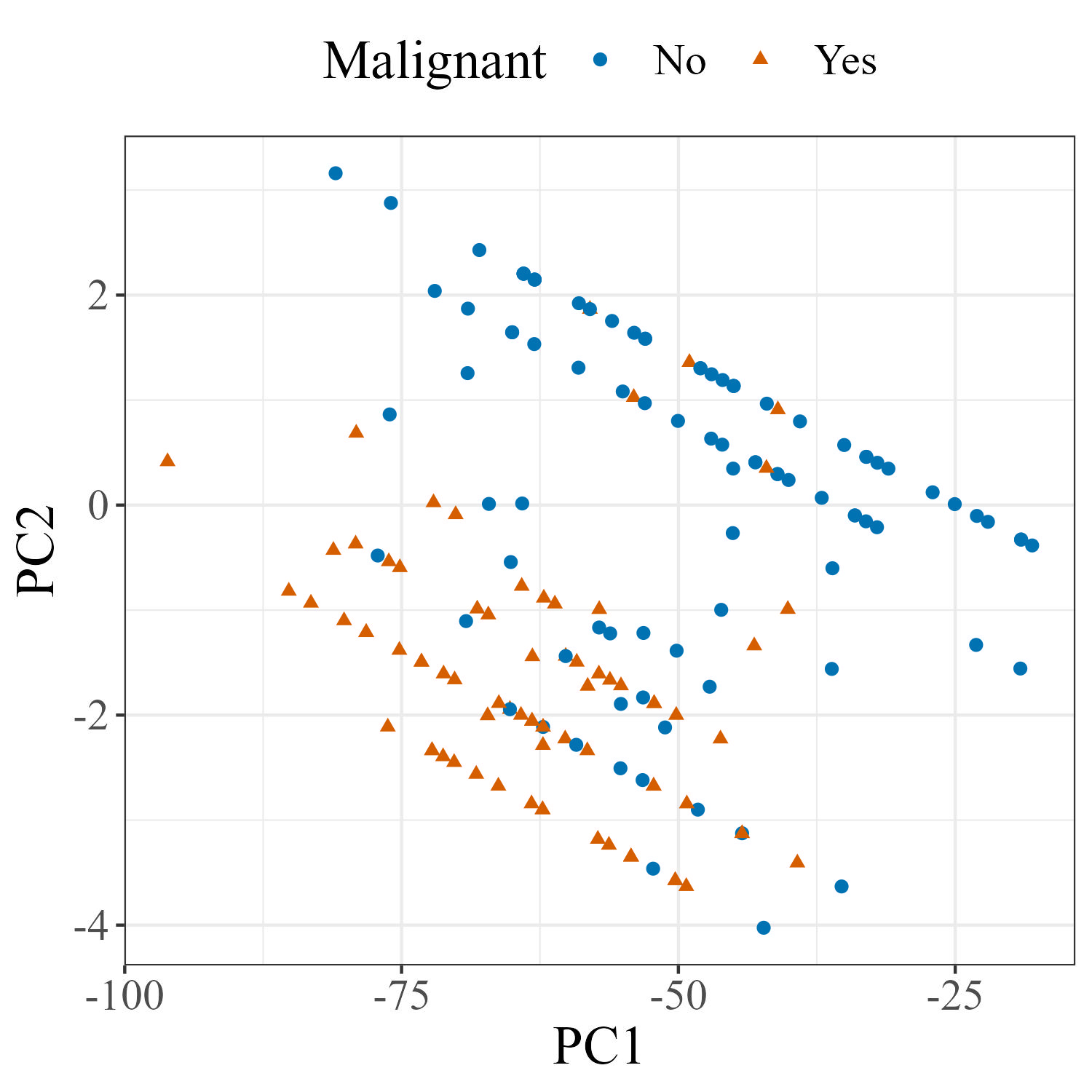
(a) Plot of the first two principal components of the mammographic mass training data. Plot depicts the separation between malignant and non-malignant masses in the reduced dimension data.

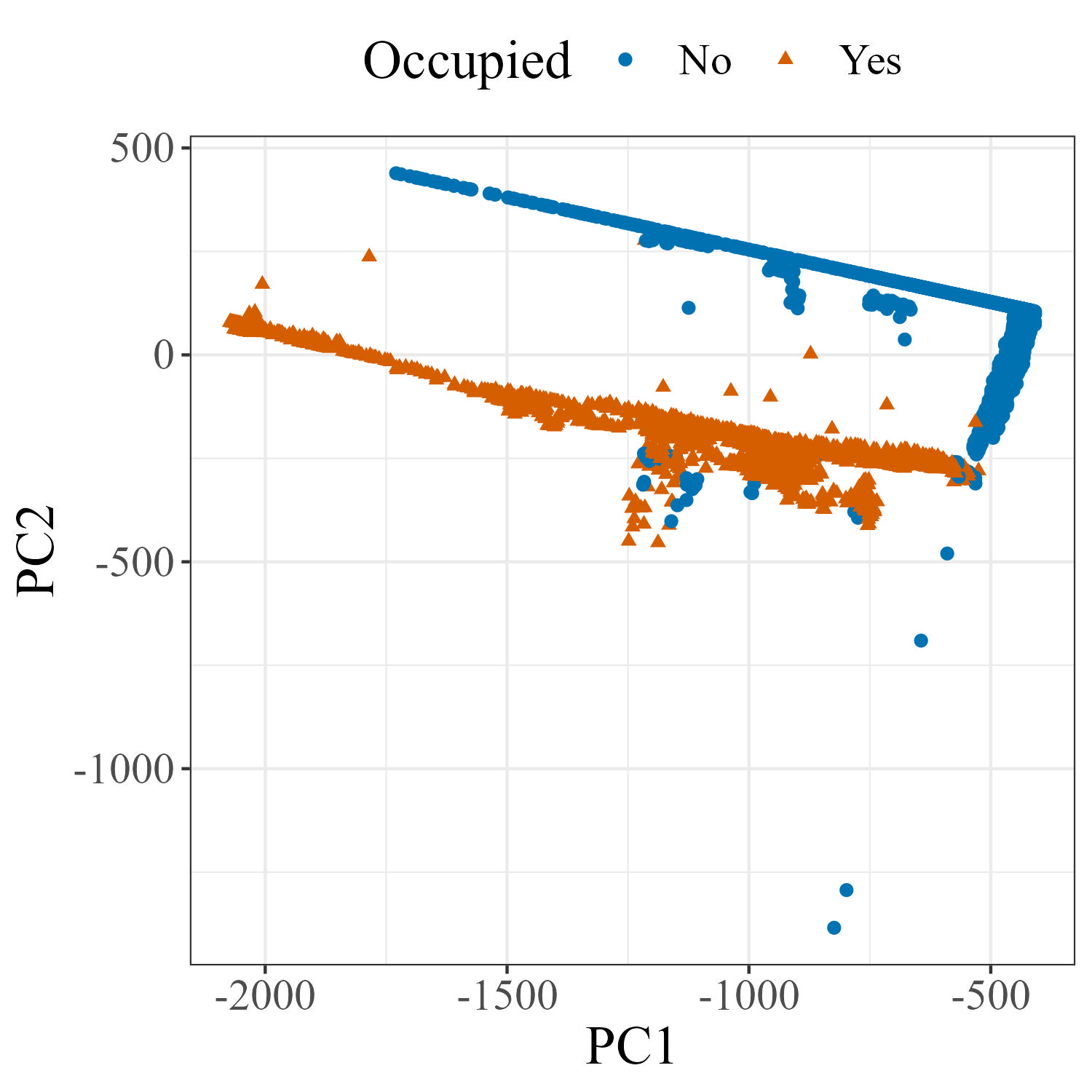
(b) Plot of the first two principal components (PC1 vs. PC2) of the occupancy detection data. Plot depicts the separation between occupied and non-occupied observations in the reduced dimension data.

Figure 1(a) depicts the first two principal components of the mammographic mass dataset. We observe relatively good linear separation between malignant and non-malignant masses in this reduced dimension in general. We randomly split the data into training (80 percent) and testing (20 percent) sets and perform 20 replicates of LDA-RK on this split so that differences among the replicates are due solely to algorithmic randomness in Algorithm 3. The resulting training and testing datasets both have rank equal to $4$ and have scaled condition numbers equal to $7{,}505$ and $7{,}312$, respectively.

Table 1 shows comparisons between LDA-GM, LDA-LS, and LDA-RK. The top portion of Table 1 shows the coefficients of the direction vectors from LDA-GM, LDA-LS, and a single replicate of LDA-RK with $c=0.9$ and $k=1{,}000{,}000$ iterations. We indicate the choice of the least squares (LS) and optimal intercepts (opt) in subscript. The middle portion shows the angles between the LDA-GM direction and the LDA-LS and LDA-RK directions. The bottom portion shows the overall and class-specific classification accuracies (with the classes denoted in subscript) of each approach including the intercept term when available. Values for the number of iterations $k$ come from an equally spaced sequence of ten numbers from $10^{3}$ to $10^{6.5}$. Therefore, $k$ ranges from $1000$ to approximately $3{,}000{,}000$.

	LDA-GM	LDA-LS${}_{\text{LS}}$	LDA-LS${}_{\text{opt}}$	Scaling	LDA-RK${}_{\text{LS}}$	LDA-RK${}_{\text{opt}}$	Scaling
Intercept		-3.17	-3.17		-3.05	-3.49
Age	0.02	0.02	0.02	0.99	0.03	0.03	0.93
Shape	0.50	0.51	0.51	0.99	0.54	0.54	0.94
Margin	0.40	0.40	0.40	0.99	0.40	0.40	1.00
Density	-0.20	-0.20	-0.20	0.99	-0.25	-0.25	0.82
Angle		0.00			3.35
Accuracy	0.80	0.79	0.79		0.79	0.80
Accuracy1	0.74	0.71	0.75		0.69	0.76
Accuracy2	0.85	0.88	0.84		0.88	0.84

Table 1: Top: Coefficients from LDA-GM, LDA-LS, and LDA-RK direction vectors with least squares (LS) and optimal (opt) intercepts denoted in subscript. Middle: Angle (degrees) from LDA-GM direction. Bottom: Overall classification accuracy and class-specific accuracies.

We observe that the LDA-LS direction vector is the same as the one from LDA-GM up to a factor of $0.99$. Therefore, LDA-GM and LDA-LS produce the same LDA directions and the angle between the two is $0$. Meanwhile, the LDA-RK direction vector after $k=1{,}000{,}000$ iterations is $3.35$ degrees away from the LDA-GM direction. Both LDA-LS and LDA-RK produce overall accuracy that is very similar to that of LDA-GM with some variation in the class-specific accuracy (Accuracy₁ and Accuracy₂ in Table 1).

Figure 2(a) depicts the mean angle (in degrees) between the LDA-GM and LDA-RK direction vectors obtained over 20 replicates as a function of the number of iterations $k$. Colored lines depict results from different step-size values $c$. While results with all step-sizes appear to approach the LDA-GM direction, larger step-sizes converge more quickly to a direction that is very close to the LDA-GM direction.

Figure 2(b) depicts the mean overall classification accuracy of the LDA-RK direction vectors obtained over 20 replicates with the optimal intercept as a function of the number of iterations $k$. Colored lines depict results from different step-size values $c$. The dashed gray line depicts the LDA-GM overall classification accuracy. Accuracy obtained with all choices of step-size $c$ approach the LDA-GM accuracy.

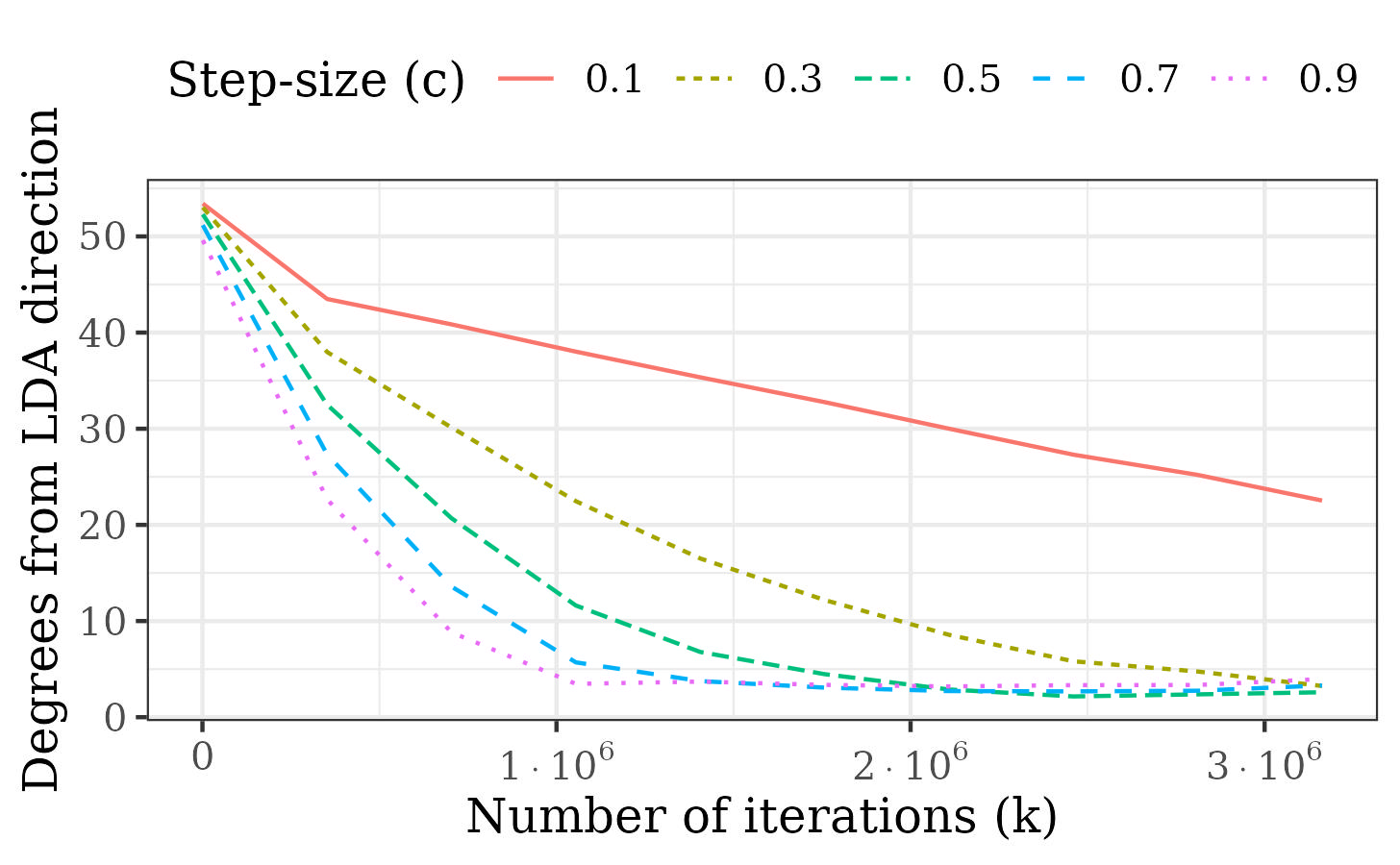
(a) Mean angle (degrees) between Gaussian model LDA and sketched LDA directions over $20$ replicates as a function of the number of iterations.

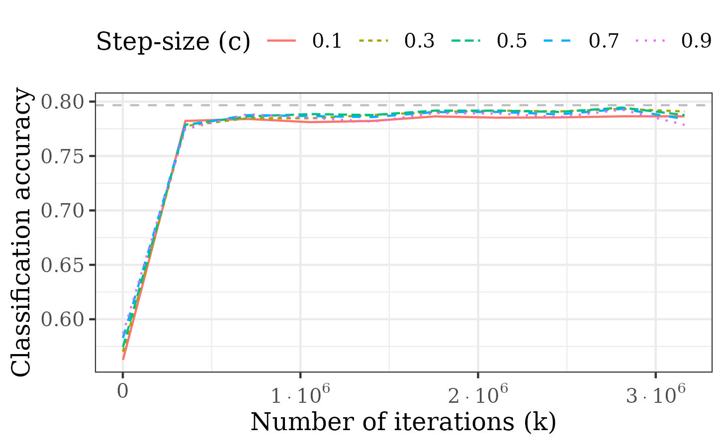
(b) Mean sketched LDA accuracy with optimal intercept over $20$ replicates as a function of the number of iterations. Gaussian model LDA accuracy ($0.797$) in gray.

These results illustrate how LDA-RK can achieve results that are very similar to that of LDA-GM while utilizing only a randomly selected row of the training data in each iteration $k$. Therefore, in data scenarios that are suitable for LDA but where the data may be too large for full data analysis, LDA-RK offers a viable alternative that performs very comparably to full data Gaussian model LDA.

4.3 Occupancy Detection Data

We also employ the occupancy detection dataset from [10] containing $8{,}143$ training and $9{,}752$ testing observations on four features: temperature (in Celsius), relative humidity (as a percent), light (in lux), and CO₂ (in ppm). The goal is to predict whether or not a room is occupied given the observed features. Figure 1(b) shows a plot of the first two principal components of the data and shows the separation between occupied and non-occupied rooms in this reduced dimension. In general, there appears to be substantial linear separation between occupied and unoccupied rooms in this reduced dimension. We perform 20 replicates of LDA-RK on the given training and testing data so that differences among the replicates are due solely to algorithmic randomness from the sampling procedure in Algorithm 3. The training and testing datasets both have rank equal to $4$ and scaled condition numbers equal to $43{,}979$ and $120{,}589$, respectively.

Table 2 shows comparisons between LDA-GM, LDA-LS, and LDA-RK. The top portion of Table 2 shows the coefficients of the direction vectors from LDA-GM, LDA-LS, and a single iterate of LDA-RK with $c=0.9$ and $k=100{,}000$ iterations. We indicate the choice of the least squares (LS) and optimal intercepts (opt) in subscript. The middle portion shows the angles between the LDA-GM direction and the LDA-LS and LDS-RK directions. The bottom portion shows the overall and class-specific classification accuracies (with the classes denoted in subscript) from each approach including the intercept term when available. Values for the number of iterations $k$ come from an equally spaced sequence of ten numbers from $10^{3}$ to $10^{6}$. Therefore, $k$ ranges from $1000$ to approximately $1{,}000{,}000$.

	LDA-GM	LDA-LS${}_{\text{LS}}$	LDA-LS${}_{\text{opt}}$	Scaling	LDA-RK${}_{\text{LS}}$	LDA-RK${}_{\text{opt}}$	Scaling
Intercept		5.65	2.86		0.94	-2.28
Temperature	-0.44	-0.38	-0.38	1.17	-0.14	-0.14	3.17
Humidity	-0.02	-0.01	-0.01	1.17	-0.01	-0.01	1.35
Light	0.01	0.01	0.01	1.17	0.01	0.01	0.99
CO2	0.00	0.00	0.00	1.17	0.00	0.00	1.78
Angle		0.00			4.63
Accuracy	0.99	0.88	0.98		0.94	0.99
Accuracy1	0.99	0.85	0.99		0.93	0.99
Accuracy2	1.00	1.00	0.93		1.00	0.99

Table 2: Top: Coefficients from LDA-GM, LDA-LS, and LDA-RK direction vectors with least squares (LS) and optimal (opt) intercepts denoted in subscript. Middle: Angle (degrees) from LDA-GM direction. Bottom: Overall classification accuracy and class-specific accuracies.

We observe that the LDA-LS direction vector is the same as the one from LDA-GM up to a scaling factor of $1.17$. Therefore, LDA-GM and LDA-LS produce the same LDA directions and the angle between the two is $0$. Meanwhile, the LDA-RK direction vector after $k=100{,}000$ iterations is $4.63$ degrees away from the LDA-GM direction. Both LDA-LS and LDA-RK produce overall accuracy that is very comparable to that of LDA-GM.

Figure 3(a) depicts the mean angle (in degrees) between the LDA-GM and LDA-RK direction vectors obtained over 20 replicates as a function of the number of iterations $k$. Colored lines depict results from different step-size values $c$. Again, we observe that results with all step-sizes appear to approach the LDA-GM direction and larger step-sizes converge more quickly to a direction that is very close to the LDA-GM direction.

Figure 3(b) depicts the mean overall classification accuracy of the LDA-RK direction vectors obtained over 20 replicates with the optimal intercept as a function of the number of iterations $k$. Colored lines depict results from different step-size values $c$ while the dashed gray line depicts the LDA-GM overall classification accuracy. Once again, the accuracy obtained with all choices of step-size $c$ approach the LDA-GM accuracy.

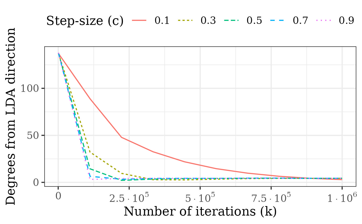
(a) Mean angle (degrees) between Gaussian model LDA and sketched LDA directions over $20$ replicates as a function of the number of iterations.

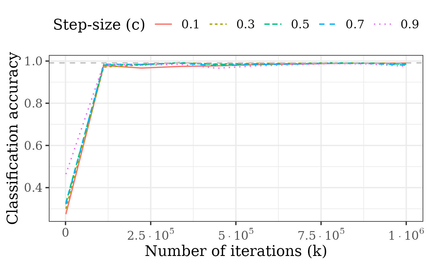
(b) Mean sketched LDA accuracy with optimal intercept over $20$ replicates as a function of the number of iterations. Gaussian model LDA accuracy ($0.991$) in gray.

These results again illustrate how LDA-RK can achieve results that are very similar to that of LDA-GM while employing only a randomly selected row of the training data in each iteration $k$. Therefore, LDA-RK offers a potent alternative to full data Gaussian model LDA when the data may be too large for full data analysis.

5 Discussion

In this work, we present sketched LDA, an iterative randomized approach to binary-class Gaussian model LDA for very large data. The keys to our method and analysis lie in harnessing the least squares formulation of binary-class Gaussian model LDA, employing the machinery of the stochastic gradient descent framework with importance sampling [53], and combining these with previous work on the statistical analysis of sketched linear regression [15]. Therefore, our convergence guarantees for the sketched LDA predictions on new data account for both the randomness from the modeling assumptions on the data and algorithmic randomness from the RK iterates.

We briefly describe how one can employ sketched LDA when the data may be too large to store in working memory on a local machine. Since Algorithm 3 only requires one row of the training data in each iteration, one may store and compute iterates on batches of sampled rows from the training data sequentially. In this way, one bypasses the need to store the full data. We note that unlike the leverage scores, the row norms and $\hat{\mathbf{\Sigma}}$ for the optimal intercept in (8) can also be computed by viewing only batches of the data sequentially. Similar to the leverage scores, however, both the row norms and $\hat{\mathbf{\Sigma}}$ would need to be computed prior to the computation of the RK iterates. The idea of viewing batches of the data in sequence is similar to that of streaming discriminant analysis [62, 35, 3]. While these are viable alternatives to full data analysis in the streaming cases, a primary difference is that these lack theoretical convergence guarantees for how close the resulting classifier is to the original full data classifier.

Finally, we conclude with some directions for future work. First, we consider the overdetermined $n>p$ case in this work but many applications, such as those in image recognition and text analysis, can involve $p>n$. This ultrahigh dimension case is a well-known problem in Gaussian model LDA since $\hat{\mathbf{\Sigma}}^{-1}$ in Algorithm 1 does not exist in this case [48] and there have been a number of works addressing this issue [5, 60, 41, 57]. Along a similar vein, a second avenue of future work would be to adapt the optimal intercept in (8) for the very large $p$ case. Since (8) involves computing $\hat{\mathbf{\Sigma}}\in\mathbb{R}^{p\times p}$, this may become computationally prohibitive for $p$ sufficiently large. One possibility may be to employ randomized approaches to computing the sample covariance. However, there exists necessary work in exploring how these approximations in the optimal intercept may influence the LDA classification accuracy.

SUPPLEMENTARY MATERIAL

Proofs:

Proofs of main results. (.pdf file)

References

- Agaskar et al., [2014] Agaskar, Ameya, Wang, Chuang, and Lu, Yue M (2014),, Randomized Kaczmarz algorithms: Exact MSE analysis and optimal sampling probabilities. in 2014 IEEE Global Conference on Signal and Information Processing (GlobalSIP), 389–393. IEEE.
- Ailon and Chazelle, [2006] Ailon, Nir and Chazelle, Bernard (2006),, Approximate nearest neighbors and the fast Johnson-Lindenstrauss transform. in Proceedings 38th Annual ACM Symp. on Theory of Computing, 557–563.
- Anagnostopoulos et al., [2012] Anagnostopoulos, Christoforos, Tasoulis, Dimitris K, Adams, Niall M, Pavlidis, Nicos G, and Hand, David J (2012), “Online linear and quadratic discriminant analysis with adaptive forgetting for streaming classification,” Statistical Analysis and Data Mining, 5, 2, 139–166.
- Avron et al., [2010] Avron, Haim, Maymounkov, Petar, and Toledo, Sivan (2010), “Blendenpik: Supercharging LAPACK’s least-squares solver,” SIAM Journal on Scientific Computing, 32, 3, 1217–1236.
- Bickel and Levina, [2004] Bickel, Peter J and Levina, Elizaveta (2004), “Some theory for Fisher’s linear discriminant function, naive Bayes’, and some alternatives when there are many more variables than observations,” Bernoulli, 10, 6, 989–1010.
- Bottou, [2010] Bottou, Léon (2010), “Large-scale machine learning with stochastic gradient descent,” In Proceedings of COMPSTAT’2010, ed. I. Proceedings of COMPSTAT’2010, Springer, pp. 177–186.
- Bottou, [2012] — (2012), “Stochastic gradient descent tricks,” In Neural Networks: Tricks of the Trade, ed. I. Neural Networks: Tricks of the Trade, Springer, pp. 421–436.
- Boutsidis and Drineas, [2009] Boutsidis, Christos and Drineas, Petros (2009), “Random projections for the nonnegative least-squares problem,” Linear Algebra and its Applications, 431, 5-7, 760–771.
- Breiman and Ihaka, [1984] Breiman, Leo and Ihaka, Ross (1984),. Nonlinear discriminant analysis via scaling and ACE. Tech. rep., Department of Statistics, University of California Davis.
- Candanedo and Feldheim, [2016] Candanedo, Luis M and Feldheim, Véronique (2016), “Accurate occupancy detection of an office room from light, temperature, humidity and CO2 measurements using statistical learning models,” Energy and Buildings, 112, 28–39.
- Censor et al., [1983] Censor, Yair, Eggermont, Paul PB, and Gordon, Dan (1983), “Strong underrelaxation in Kaczmarz’s method for inconsistent systems,” Numerische Mathematik, 41, 1, 83–92.
- Censor et al., [2009] Censor, Yair, Herman, Gabor T, and Jiang, Ming (2009), “A note on the behavior of the randomized Kaczmarz algorithm of Strohmer and Vershynin,” Journal of Fourier Analysis and Applications, 15, 4, 431–436.
- Chatterjee and Hadi, [1986] Chatterjee, Samprit and Hadi, Ali S (1986), “Influential observations, high leverage points, and outliers in linear regression,” Statistical Science, 379–393.
- Chi and Ipsen, [2021] Chi, Jocelyn T. and Ipsen, Ilse C. F. (2021), “Multiplicative Perturbation Bounds for Multivariate Multiple Linear Regression in Schatten -Norms,” Linear Algebra and its Applications, 624, 87–102.
- Chi and Ipsen, [2022] — (2022), “A Projector-Based Approach to Quantifying Total and Excess Uncertainties for Sketched Linear Regression,” Information and Inference, 11, 1055–1077.
- Cooke, [2002] Cooke, Tristrom (2002), “Two variations on Fisher’s linear discriminant for pattern recognition,” IEEE Transactions on Pattern Analysis and Machine Intelligence, 24, 2, 268–273.
- Dai et al., [2013] Dai, Liang, Soltanalian, Mojtaba, and Pelckmans, Kristiaan (2013), “On the randomized Kaczmarz algorithm,” IEEE Signal Processing Letters, 21, 3, 330–333.
- Davidson and Szarek, [2001] Davidson, Kenneth R and Szarek, Stanislaw J (2001), “Local operator theory, random matrices and Banach spaces,” Handbook of the Geometry of Banach Spaces, 1, 317-366, 131.
- De Loera et al., [2017] De Loera, Jesus A, Haddock, Jamie, and Needell, Deanna (2017), “A sampling Kaczmarz–Motzkin algorithm for linear feasibility,” SIAM Journal on Scientific Computing, 39, 5, S66–S87.
- Demmel, [1988] Demmel, James W (1988), “The probability that a numerical analysis problem is difficult,” Mathematics of Computation, 50, 182, 449–480.
- Drineas et al., [2012] Drineas, Petros, Magdon-Ismail, Malik, Mahoney, Michael W, and Woodruff, David P (2012), “Fast approximation of matrix coherence and statistical leverage,” The Journal of Machine Learning Research, 13, 1, 3475–3506.
- Drineas et al., [2006] Drineas, P., Mahoney, M. W., and Muthukrishnan, S. (2006),, Sampling algorithms for regression and applications. in Proceedings of the 17th Annual ACM-SIAM Symposium on Discrete Algorithms, 1127–1136. ACM, New York.
- Drineas et al., [2011] Drineas, P., Mahoney, M. W., Muthukrishnan, S., and Sarlós, T. (2011), “Faster least squares approximation,” Numerische Mathematik, 117, 219–249.
- Du, [2007] Du, Qian (2007), “Modified Fisher’s linear discriminant analysis for hyperspectral imagery,” IEEE Geoscience and Remote Sensing letters, 4, 4, 503–507.
- Durrant and Kabán, [2010] Durrant, Robert J and Kabán, Ata (2010),, Compressed Fisher linear discriminant analysis: Classification of randomly projected data. in Proceedings of the 16th ACM SIGKDD International Conference on Knowledge Siscovery and Data Mining, 1119–1128.
- Durrant and Kabán, [2015] — (2015), “Random projections as regularizers: Learning a linear discriminant from fewer observations than dimensions,” Journal of Machine Learning Research, 99, 2, 257–286.
- Edelman, [1989] Edelman, Alan (1989), Eigenvalues and Condition Numbers of Random Matrices, D.Phil. thesis, Yale University.
- Elter et al., [2007] Elter, Matthias, Schulz-Wendtland, Rüdiger, and Wittenberg, Thomas (2007), “The prediction of breast cancer biopsy outcomes using two CAD approaches that both emphasize an intelligible decision process,” Medical Physics, 34, 11, 4164–4172.
- Fisher, [1936] Fisher, Ronald A (1936), “The use of multiple measurements in taxonomic problems,” Annals of Eugenics, 7, 2, 179–188.
- Gower et al., [2019] Gower, Robert, Molitor, Denali, Moorman, Jacob, and Needell, Deanna (2019), “Adaptive sketch-and-project methods for solving linear systems,”.
- Gower and Richtárik, [2015] Gower, Robert M and Richtárik, Peter (2015), “Randomized iterative methods for linear systems,” SIAM Journal on Matrix Analysis and Applications, 36, 4, 1660–1690.
- Guimet et al., [2006] Guimet, Francesca, Boqué, Ricard, and Ferré, Joan (2006), “Application of non-negative matrix factorization combined with Fisher’s linear discriminant analysis for classification of olive oil excitation–emission fluorescence spectra,” Chemometrics and Intelligent Lab. Systems, 81, 1, 94–106.
- Hanke and Niethammer, [1990] Hanke, Martin and Niethammer, Wilhelm (1990), “On the acceleration of Kaczmarz’s method for inconsistent linear systems,” Linear Algebra and its Applications, 130, 83–98.
- Hastie et al., [2009] Hastie, Trevor, Tibshirani, Robert, and Friedman, Jerome (2009), The elements of statistical learning: data mining, inference, and prediction, Springer Science & Business Media.
- Hayes and Kanan, [2020] Hayes, Tyler L and Kanan, Christopher (2020),, Lifelong machine learning with deep streaming linear discriminant analysis. in Proceedings of the IEEE/CVF Conference on Computer Vision and Pattern Recognition Workshops, 220–221.
- Hoaglin and Welsch, [1978] Hoaglin, David C and Welsch, Roy E (1978), “The hat matrix in regression and ANOVA,” The American Statistician, 32, 1, 17–22.
- Ipsen and Wentworth, [2014] Ipsen, Ilse CF and Wentworth, Thomas (2014), “The effect of coherence on sampling from matrices with orthonormal columns, and preconditioned least squares problems,” SIAM Journal on Matrix Analysis and Applications, 35, 4, 1490–1520.
- Kabán, [2014] Kabán, Ata (2014),, New bounds on compressive linear least squares regression. in Artificial Intelligence and Statistics, 448–456. PMLR.
- Kaczmarz, [1937] Kaczmarz, S (1937), “Angenaherte auflosung von systemen linearer gleichungen: Bulletin international de l’académie polonaise des sciences et des lettres,” Classe des Sciences Mathématiques et Naturelles. Série A, Sciences Mathématiques, 35, 355–357.
- Khaled et al., [2020] Khaled, Ahmed, Sebbouh, Othmane, Loizou, Nicolas, Gower, Robert M, and Richtárik, Peter (2020), “Unified analysis of stochastic gradient methods for composite convex and smooth optimization,” arXiv preprint arXiv:2006.11573.
- Li et al., [2019] Li, Yanming, Hong, Hyokyoung G, and Li, Yi (2019), “Multiclass linear discriminant analysis with ultrahigh-dimensional features,” Biometrics, 75, 4, 1086–1097.
- Lin and Zhou, [2015] Lin, Junhong and Zhou, Ding-Xuan (2015), “Learning theory of randomized Kaczmarz algorithm,” The Journal of Machine Learning Research, 16, 1, 3341–3365.
- Liu and Wechsler, [1998] Liu, Chengjun and Wechsler, Harry (1998),, Enhanced Fisher linear discriminant models for face recognition. in Proceedings. Fourteenth International Conference on Pattern Recognition (Cat. No. 98EX170), vol. 2, 1368–1372. IEEE.
- Liu and Wechsler, [2002] — (2002), “Gabor feature based classification using the enhanced Fisher linear discriminant model for face recognition,” IEEE Transactions on Image Processing, 11, 4, 467–476.
- Liu and Wright, [2016] Liu, Ji and Wright, Stephen (2016), “An accelerated randomized Kaczmarz algorithm,” Mathematics of Computation, 85, 297, 153–178.
- Liu et al., [2014] Liu, Ji, Wright, Stephen J, and Sridhar, Srikrishna (2014), “An asynchronous parallel randomized Kaczmarz algorithm,” arXiv preprint arXiv:1401.4780.
- Ma et al., [2015] Ma, P., Mahoney, M. W., and Yu, B. (2015), “A statistical perspective on algorithmic leveraging,” Journal of Machine Learning Research, 16, 861–911.
- Mai, [2013] Mai, Qing (2013), “A review of discriminant analysis in high dimensions,” Wiley Interdisciplinary Reviews: Computational Statistics, 5, 3, 190–197.
- Mai et al., [2012] Mai, Qing, Zou, Hui, and Yuan, Ming (2012), “A direct approach to sparse discriminant analysis in ultra-high dimensions,” Biometrika, 99, 1, 29–42.
- Maillard and Munos, [2009] Maillard, Odalric and Munos, Rémi (2009), “Compressed least-squares regression,” Advances in Neural Information Processing Systems, 22.
- Meng et al., [2014] Meng, X., Saunders, M. A., and Mahoney, M. W. (2014), “LSRN: a parallel iterative solver for strongly over- or underdetermined systems,” SIAM Journal on Scientific Computing, 36, 2, C95–C118.
- Needell, [2010] Needell, Deanna (2010), “Randomized Kaczmarz solver for noisy linear systems,” BIT Numerical Mathematics, 50, 2, 395–403.
- Needell et al., [2016] Needell, Deanna, Srebro, Nathan, and Ward, Rachel (2016), “Stochastic gradient descent, weighted sampling, and the randomized Kaczmarz algorithm,” Mathematical Programming, 155, 1-2, 549–573.
- Needell and Ward, [2013] Needell, Deanna and Ward, Rachel (2013), “Two-subspace projection method for coherent overdetermined systems,” Journal of Fourier Analysis and Applications, 19, 2, 256–269.
- Nemirovski et al., [2009] Nemirovski, Arkadi, Juditsky, Anatoli, Lan, Guanghui, and Shapiro, Alexander (2009), “Robust stochastic approximation approach to stochastic programming,” SIAM Journal on Optimization, 19, 4, 1574–1609.
- Nesterov, [2012] Nesterov, Yu (2012), “Efficiency of coordinate descent methods on huge-scale optimization problems,” SIAM Journal on Optimization, 22, 2, 341–362.
- Ni and Fang, [2016] Ni, Lyu and Fang, Fang (2016), “Entropy-based model-free feature screening for ultrahigh-dimensional multiclass classification,” Journal of Nonparametric Statistics, 28, 3, 515–530.
- Niu and Zheng, [2020] Niu, Yu-Qi and Zheng, Bing (2020), “A greedy block Kaczmarz algorithm for solving large-scale linear systems,” Applied Mathematics Letters, 104, 106294.
- Nutini et al., [2016] Nutini, Julie, Sepehry, Behrooz, Laradji, Issam, Schmidt, Mark, Koepke, Hoyt, and Virani, Alim (2016), “Convergence rates for greedy Kaczmarz algorithms, and faster randomized Kaczmarz rules using the orthogonality graph,” arXiv preprint arXiv:1612.07838.
- Pan et al., [2016] Pan, Rui, Wang, Hansheng, and Li, Runze (2016), “Ultrahigh-dimensional multiclass linear discriminant analysis by pairwise sure independence screening,” Journal of the American Statistical Association, 111, 513, 169–179.
- Pan and Chen, [1999] Pan, Victor Y and Chen, Zhao Q (1999),, The complexity of the matrix eigenproblem. in Proceedings of the 31st Annual ACM Symposium on Theory of Computing, 507–516.
- Pang et al., [2005] Pang, Shaoning, Ozawa, Seiichi, and Kasabov, Nikola (2005), “Incremental linear discriminant analysis for classification of data streams,” IEEE Trans. on Systems, Man, and Cybernetics (B), 35, 5, 905–914.
- Papailiopoulos et al., [2014] Papailiopoulos, Dimitris, Kyrillidis, Anastasios, and Boutsidis, Christos (2014),, Provable deterministic leverage score sampling. in Proceedings 20th ACM SIGKDD International Conference on Knowledge Discovery and Data Mining, 997–1006.
- Raskutti and Mahoney, [2016] Raskutti, G. and Mahoney, M. W. (2016), “A statistical perspective on randomized sketching for ordinary least-squares,” Journal of Machine Learning Research, 17, 1, 7508–7538.
- Rebrova and Needell, [2020] Rebrova, Elizaveta and Needell, Deanna (2020), “On block Gaussian sketching for the Kaczmarz method,” Numerical Algorithms, 1–31.
- Richtárik and Takáč, [2014] Richtárik, Peter and Takáč, Martin (2014), “Iteration complexity of randomized block-coordinate descent methods for minimizing a composite function,” Mathematical Programming, 144, 1, 1–38.
- Ripley, [2007] Ripley, Brian D (2007), Pattern recognition and neural networks, Cambridge university press.
- Robbins and Monro, [1951] Robbins, Herbert and Monro, Sutton (1951), “A stochastic approximation method,” The Annals of Mathematical Statistics, 400–407.
- Rokhlin and Tygert, [2008] Rokhlin, V. and Tygert, M. (2008), “A fast randomized algorithm for overdetermined linear least-squares regression,” Proceedings of the National Academy of Sciences USA, 105, 36, 13212–13217.
- Sarlos, [2006] Sarlos, Tamas (2006),, Improved approximation algorithms for large matrices via random projections. in 2006 47th annual IEEE symposium on foundations of computer science (FOCS’06), 143–152. IEEE.
- Steinerberger, [2021] Steinerberger, Stefan (2021), “A weighted randomized Kaczmarz method for solving linear systems,” Mathematics of Computation, 90, 332, 2815–2826.
- Strohmer and Vershynin, [2009] Strohmer, Thomas and Vershynin, Roman (2009), “A randomized Kaczmarz algorithm with exponential convergence,” Journal of Fourier Analysis and Applications, 15, 2, 262.
- Tanabe, [1971] Tanabe, Kunio (1971), “Projection method for solving a singular system of linear equations and its applications,” Numerische Mathematik, 17, 3, 203–214.
- Thanei et al., [2017] Thanei, Gian-Andrea, Heinze, Christina, and Meinshausen, Nicolai (2017), “Random projections for large-scale regression,” In Big and complex data analysis, ed. I. Big and complex data analysis, Springer, pp. 51–68.
- Velleman and Welsch, [1981] Velleman, Paul F and Welsch, Roy E (1981), “Efficient computing of regression diagnostics,” The American Statistician, 35, 4, 234–242.
- Whitney and Meany, [1967] Whitney, TM and Meany, RK (1967), “Two algorithms related to the method of steepest descent,” SIAM journal on Numerical Analysis, 4, 1, 109–118.
- Witten and Tibshirani, [2011] Witten, Daniela M and Tibshirani, Robert (2011), “Penalized classification using Fisher’s linear discriminant,” Journal of the Royal Statistical Society: Series B, 73, 5, 753–772.
- Woodruff et al., [2014] Woodruff, David P et al. (2014), “Sketching as a tool for numerical linear algebra,” Foundations and Trends® in Theoretical Computer Science, 10, 1–2, 1–157.
- Xiong et al., [2000] Xiong, Momiao, Jin, Li, Li, Wuju, and Boerwinkle, Eric (2000), “Computational methods for gene expression-based tumor classification,” Biotechniques, 29, 6, 1264–1270.
- Ye et al., [2017] Ye, Haishan, Li, Yujun, Chen, Cheng, and Zhang, Zhihua (2017), “Fast Fisher discriminant analysis with randomized algorithms,” Pattern Recognition, 72, 82–92.
- Ye, [2007] Ye, Jieping (2007),, Least squares linear discriminant analysis. in Proceedings of the 24th international conference on Machine learning, 1087–1093.
- Zhou et al., [2007] Zhou, Shuheng, Wasserman, Larry, and Lafferty, John (2007), “Compressed regression,” Advances in Neural Information Processing Systems, 20.
- Zouzias and Freris, [2013] Zouzias, Anastasios and Freris, Nikolaos M (2013), “Randomized extended Kaczmarz for solving least squares,” SIAM Journal on Matrix Analysis and Applications, 34, 2, 773–793.