A Randomised Subspace Gauss-Newton Method for Nonlinear Least-Squares

Abstract

We propose a Randomised Subspace Gauss-Newton (R-SGN) algorithm for solving nonlinear least-squares optimization problems, that uses a sketched Jacobian of the residual in the variable domain and solves a reduced linear least-squares on each iteration. A sublinear global rate of convergence result is presented for a trust-region variant of R-SGN, with high probability, which matches deterministic counterpart results in the order of the accuracy tolerance. Promising preliminary numerical results are presented for R-SGN on logistic regression and on nonlinear regression problems from the CUTEst collection.

1 Introduction

We aim to solve the nonlinear least-squares problem

$$\min_{x\in\mathbb{R}^{d}}f(x)=\frac{1}{2}\sum_{i=1}^{n}\norm{r_{i}(x)}_{2}^{2}=\frac{1}{2}\|r(x)\|_{2}^{2}$$ (1)

where $r=(r_{1},\dots,r_{n}):\mathbb{R}^{d}\to\mathbb{R}^{n}$ is a smooth vector of nonlinear (possibly nonconvex) residual functions. We define the Jacobian (matrix of first order derivatives) as

$$J(x)=\left(\partialderivative{r_{i}(x)}{x_{j}}\right)_{ij}\in\mathbb{R}^{n\times d}$$

and can then compactly write the gradient as $\gradient f(x)=J(x)^{T}r(x)$. The classical Gauss-Newton (GN) algorithm simply applies Newton’s method to minimising $f$ with only the first-order $J(x)^{T}J(x)$ term in the Hessian, dropping the second-order terms involving the Hessians of the residuals $r_{i}$. Thus, at every iterate $x_{k}$, Gauss-Newton approximately minimises the following convex quadratic local model

$$f(x_{k})+\langle J(x_{k})^{T}r(x_{k}),\hat{s}\rangle+\frac{1}{2}\langle\hat{s},J(x_{k})^{T}J(x_{k})\hat{s}\rangle$$

over $\hat{s}\in\mathbb{R}^{d}$. In our approach, which we call Randomised Subspace Gauss-Newton (R-SGN), we reduce the dimensionality of this model by minimising in an $l$-dimensional randomised subspace $\mathcal{L}\subset\mathbb{R}^{d}$, with $l\ll d$, by approximately minimising the following reduced model

$$f(x_{k})+\langle J_{\mathcal{S}}(x_{k})^{T}r(x_{k}),s\rangle+\frac{1}{2}\langle s,J_{\mathcal{S}}(x_{k})^{T}J_{\mathcal{S}}(x_{k})s\rangle$$ (2)

over $s\in\mathbb{R}^{l}$, where $J_{\mathcal{S}}(x_{k})\in\mathbb{R}^{n\times l}$ denotes the reduced Jacobian. Compared to the classical Gauss-Newton model, this reduced model also offers the computational advantage that it only needs to evaluate $l$ Jacobian actions, giving $J_{\mathcal{S}}(x_{k})$, instead of the full Jacobian matrix $J(x_{k})$.

In its simplest form, $J_{\mathcal{S}}$ can be thought of as a random subselection of columns of the full Jacobian $J$, which leads to variants of our framework that are Block-Coordinate Gauss-Newton (BC-GN) methods. In this case, for example, if the Jacobian were being calculated by finite-differences of the residual $r$, only a small number of evaluations of $r$ along coordinate directions would be needed; such a BC-GN variant has already been used for parameter estimation in climate modelling (Tett et al., 2017).

2 Related Work and Motivation

Block-coordinate descent methods have been, by now, extensively studied, especially for minimizing convex functions (Richtárik & Takáč, 2014), but not only; the randomised nonmonotone block proximal-gradient method (Lu & Xiao, 2017) minimises the sum of a smooth (possibly nonconvex) function and a block-separable (possibly nonconvex nonsmooth) function, with global rates of convergence being provided for when the expected value of the (true) gradient is sufficiently small. In a similar vein, Facchinei et al. (2015) propose a general decomposition framework for the parallel optimization of the sum of a smooth (possibly nonconvex) function and a block-separable nonsmooth convex function. Both of these proposals are gradient descent frameworks, while for improved and robust practical performance, (some) second-order information of the objective function needs to be employed in the algorithm. As second-order methods may be too computationally expensive for large-scale applications, subspace variants have been devised; extensive literature exists on deterministic choices such as Newton-CG (conjugate gradient) and Krylov methods, both for calculating approximate Newton directions for general optimization and approximate Gauss-Newton directions for nonlinear least-squares (see for example, Nocedal & Wright, 2006; Gratton et al., 2007). However, though these methods are really powerful and very much state-of-the-art for inexact second-order methods, they still require (full) Hessian-vector products, which may be too expensive for some applications (Tett et al., 2017). Also, we are interested in using randomisation techniques for choosing the subspace of minimization, in an attempt to exploit the benefits of Johnson-Lindenstrauss (JL) Lemma-like results, that essentially reduce the dimension of the optimization problem without loss of information. Such sketching techniques have already been proposed, especially for convex optimization, as we describe next. The sketched Newton algorithm (Pilanci & Wainwright, 2017) requires a sketching matrix that is proportional to the rank of the Hessian, which may be too computationally expensive. By contrast, sketched online Newton (Luo et al., 2016) uses streaming sketches to scale up a second-order method, comparable to Gauss–Newton, for solving online learning problems. The randomised subspace Newton (Gower et al., 2019) efficiently sketches the full Newton direction for a family of generalised linear models, such as logistic regression. The stochastic dual Newton ascent algorithm in Qu et al. (2016) requires a positive definite upper bound $M$ on the Hessian and proceeds by selecting random principal submatrices of $M$ that are then used to form and solve an approximate Newton system. The randomized block cubic Newton method in Doikov & Richtárik (2018) combines the ideas of randomized coordinate descent with cubic regularization and requires the optimization problem to be block separable.

Here, we propose a randomized subspace Gauss-Newton method for nonlinear least-squares problems, that, at each iteration, only needs a sketch of the Jacobian matrix in the variable domain, which it then uses to solve a reduced linear least-squares problem for the step calculation. To ensure global convergence of the method, from any starting point, we include a trust-region technique (and also have results for a quadratic regularization variant); unlike most prior work, we focus on the general nonconvex case of problem (1).

3 The R-SGN Algorithm

As mentioned above, at each iterate $x_{k}$, $k\geq 0$, R-SGN uses Jacobian actions $J_{\mathcal{S}}(x_{k})$ in an $l$-dimensional randomised subspace $\mathcal{L}\subset\mathbb{R}^{d}$, $l\ll d$. To obtain these actions we draw a random sketching matrix $S_{k}\in\mathbb{R}^{l\times d}$ from a chosen random matrix distribution $\mathcal{S}$ at each iteration, and set

$$J_{\mathcal{S}}(x_{k})\mathrel{\mathop{:}}=J(x_{k})S_{k}^{T}$$

in the local model (2). This model is then approximately minimized over a trust region ball, $\norm{s}_{2}\leq\Delta_{k}$, so that a typical Cauchy decrease condition (see e.g. Conn et al., 2000) is satisfied,

$$m_{k}(0)-m_{k}(s_{k})\geq c_{1}\|g_{k}\|_{2}\min\left(\Delta_{k},\frac{\|g_{k}\|_{2}}{\|B_{k}\|_{2}}\right),$$ (3)

for some constant $c_{1}>0$; where $g_{k}\mathrel{\mathop{:}}=J_{\mathcal{S}}(x_{k})^{T}r(x_{k})$ and $B_{k}\mathrel{\mathop{:}}=J_{\mathcal{S}}(x_{k})^{T}J_{\mathcal{S}}(x_{k})$. The step is then either accepted or rejected depending on the ratio $\rho_{k}$ between the actual objective decrease and the decrease predicted by the model,

$$\rho_{k}\mathrel{\mathop{:}}=\frac{f(x_{k})-f(x_{k}+S_{k}^{T}s_{k})}{f(x_{k})-m_{k}(s_{k})}.$$ (4)

A full description of the R-SGN with trust region algorithm is provided in Algorithm 1 below.

Algorithm 1 R-SGN with Trust Region

  Input: $x_{0}\in\mathbb{R}^{d}$

  Parameters: $l<d$, $\eta\in(0,1)$, $0<\gamma_{1}<1<\gamma_{2}$, such that $\gamma_{2}=\gamma_{1}^{-c}$ for some $c\in\mathbb{N}$, $\Delta_{0}\in\mathbb{R}$.

  for $k=0$ to $N$ do

     Randomly draw a sketching matrix $S_{k}\in\mathbb{R}^{l\times d}$.

      Compute step $s_{k}$ to approximately minimise the model (2) satisfying (3).

      Compute decrease $\rho_{k}$ given by (4).

     if $\rho_{k}\geq\eta$ then

        $x_{k+1}=x_{k}+S_{k}^{T}s_{k}$

        $\Delta_{k+1}=\gamma_{2}\Delta_{k}$

     else

        $\Delta_{k+1}=\gamma_{1}\Delta_{k}$

     end if

  end for

4 A global rate of convergence for R-SGN

We assume the following properties of the residual $r(x)$, the Jacobian $J(x)$ and the random sketching matrices $S_{k}$.

Assumption 1.

The residual $r$ is continuously differentiable, and $r$ and its Jacobian $J$ are Lipschitz continuous on $\mathbb{R}^{d}$.

Assumption 2.

Let $\epsilon_{S},\delta_{S}\in(0,1)$. At each iterate $x_{k}$, with probability at least $1-\delta_{S}$, we have that

$$\|S_{k}\gradient f(x_{k})\|_{2}^{2}\geq(1-\epsilon_{S})\|\gradient f(x_{k})\|_{2}^{2},$$ (5)

and

$$\|S_{k}\|_{2}\leq S_{max}.$$ (6)

Assumption 3.

The probability in Assumption 2 satisfies

$$1-\delta_{S}>c_{2},$$ (7)

where $c_{2}=\frac{c+2}{2c+2}$, with $c$ being a user chosen parameter defined in Algorithm 1. If $c=1$, i.e. we have $\gamma_{2}=\gamma_{1}^{-1}$ in Algorithm 1, then $c_{2}=3/4$.

The following result shows that the R-SGN algorithm produces an iterate with arbitrarily small $\|\gradient f(x_{k})\|_{2}$, with exponentially small failure probability, in a quantifiable number of iterations.

Theorem 1.

Let Assumptions 1, 2, 3 hold. Let $\epsilon>0$, and $\delta_{1}\in(0,1)$ such that $(1-\delta_{S})(1-\delta_{1})>c_{2}$. Then the R-SGN algorithm takes at most

$$N\leq\frac{1}{(1-\delta_{S})(1-\delta_{1})-c_{2}}\mathcal{O}\left(\frac{f(x_{0})-f^{*}}{(1-\epsilon_{S})\epsilon^{2}}\right)$$ (8)

iterations and evaluations of the residual and sketched Jacobian such that $\min_{k\leq N}\|\gradient f(x_{k})\|_{2}\leq\epsilon$, with probability at least $1-e^{-\frac{\delta_{1}^{2}}{2}(1-\delta_{S})N}$.

We note that as a function of the tolerance $\epsilon$, this bound matches deterministic complexity bounds for first-order and Gauss-Newton methods (Cartis et al., 2012), despite having only partial Jacobian information available at each iteration.

We also have similar global rates of convergence results for R-SGN with quadratic regularization techniques instead of trust region. There is no convexity or special structure requirement on $f$ or $r$ in our results. Our proof employs techniques from convergence/complexity analysis of optimisation methods based on probabilistic models in Cartis & Scheinberg (2018); Gratton et al. (2018). However, our result only assumes a weaker condition, namely, that the ’model gradient’ $S_{k}\gradient f(x_{k})$ has similar norm to that of the full gradient $\gradient f(x_{k})$, while previous results assume the model gradient itself approximates the true gradient.

4.1 Discussion on generating the random matrix $S_{k}$

We give a few suitable choices of the random matrix ensemble $\cal{S}$ satisfying Assumption 2.

Definition 1 (Non-uniformity dependent oblivious JL embedding).

Let $\epsilon_{S},\delta_{S}\in(0,1)$, $\nu_{S}\in(0,1]$, $d\in\mathbb{N}$. A distribution on $S\in\mathbb{R}^{l\times d}$ with $l=l(d,\nu_{S},\epsilon_{S},\delta_{S})$ is a $(\nu_{S},\epsilon_{S},\delta_{S})$-oblivious JL embedding if, given fixed $y\in\mathbb{R}^{d}$ with $\|y\|_{\infty}/\|y\|_{2}\leq\nu_{S}$, we have that with probability at least $1-\delta_{S}$, a matrix $S$ drawn from the distribution satisfies

$$(1-\epsilon_{S})\|y\|_{2}^{2}\leq\|Sy\|_{2}^{2}\leq(1+\epsilon_{S})\|y\|_{2}^{2}.$$ (9)

Thus we can satisfy (5) with probability at least $1-\delta_{S}$ at each R-SGN iteration if our random matrix distribution $\cal{S}$ is a $(\nu_{S},\epsilon_{S},\delta_{S})$-oblivious JL embedding, and we have that $\|\gradient f(x_{k})\|_{\infty}/\|\gradient f(x_{k})\|_{2}\leq\nu_{S}$ for all iterates $x_{k}$ by taking $y=\gradient f(x_{k})$ in Definition 1.

The well studied oblivious JL-embedding (see Woodruff, 2014), is a special case of Definition 1 with $\nu_{S}=1$. In particular, we have the following result.

Lemma 1 (Dasgupta & Gupta, 2003).

We say $S\in\mathbb{R}^{l\times d}$ is a Gaussian matrix if $S_{ij}$ are identically distributed as $N(0,{l}^{-1/2})$. Let $\epsilon_{S},\delta_{S}\in(0,1)$, then the distribution of Gaussian matrices $S\in\mathbb{R}^{l\times d}$ with $l=\mathcal{O}(|\log\delta_{S}|/\epsilon_{S}^{2})$ is an $(1,\epsilon_{S},\delta_{S})$-oblivious JL embedding.

The following hashing/sparse embedding matrices are also $(1,\epsilon_{S},\delta_{S})$-oblivious JL embeddings.

Lemma 2 (Kane & Nelson, 2014; Cohen et al., 2018).

We define $S\in\mathbb{R}^{l\times d}$ to be a s-hashing matrix if, independently for each $j\in[d]$, we sample without replacement $i_{1},i_{2},\dots,i_{s}\in[l]$ uniformly at random and let $S_{i_{k}j}=\pm 1/\sqrt{s}$, $k=1,2,\dots,s$. Let $\epsilon_{S},\delta_{S}\in(0,1)$, then the distribution of s-hashing matrices $S\in\mathbb{R}^{l\times d}$ with $s=\mathcal{O}(|\log\delta_{S}|/\epsilon_{S})$ and $l=\mathcal{O}\left(|\log\delta_{S}|/\epsilon_{S}^{2}\right)$ is an $(1,\epsilon_{S},\delta_{S})$-oblivious JL embedding.

The distribution of sampling matrices is not usually an oblivious JL embedding. However it can be shown to be a non-uniformity dependent oblivious JL embedding.

Lemma 3.

We define $S\in\mathbb{R}^{l\times d}$ to be a sampling matrix if, independently for each $i\in[l]$, we sample $j\in[d]$ uniformly at random and let $S_{ij}=(d/l)^{-1/2}$. Let $\epsilon_{S},\delta_{S},\nu_{S}\in(0,1)$, then the distribution of sampling matrices $S\in\mathbb{R}^{l\times d}$ with $l=\mathcal{O}(d\nu_{S}^{2}|\log\delta_{S}|/\epsilon_{S}^{2})$ is an $(\epsilon_{S},\delta_{S},\nu_{S})$-oblivious JL embedding.

Note that R-SGN with a sampling choice for $S_{k}$ leads to block-coordinate variants (BC-GN) of R-SGN, with fixed block size $l$.

The above properties of Gaussian and hashing matrices imply that their embedding dimension $l$ is independent of the variable dimension $d$, while for sampling matrices $l\propto d\nu_{S}^{2}$; this has direct implications on the size of the sketch in R-SGN; in particular, it does not have to grow asymptotically. However, when $\|\gradient f(x_{k})\|_{\infty}\leq Cd^{-1/2}\|\gradient f(x_{k})\|_{2}$ for some constant $C$ (thus the maximum gradient component is no larger than a constant multiple of the average gradient component), then sampling matrices also have an embedding dimension $l$ that is independent of the variable dimension $d$. Thus the more uniformly distributed the magnitude of the gradient entries, the better sampling works in R-SGN (namely, in BC-GN), ensuring a.s. global convergence.

It can be easily verified that (6) is satisfied for sampling and hashing matrices. For Gaussian matrices, one may use the non-asymptotic bound established for the maximum singular value of Gaussian matrices in Rudelson & Vershynin (2010) to show $\|S_{k}\|_{2}$ is bounded with high probability. Assumption 2 can then be satisfied with a union bound.

5 Preliminary Numerical Results

For simplicity, in our performance evaluation of R-SGN, we use sampling sketching matrices as defined in Lemma 3, which leads to a BC-GN variant of R-SGN. We first consider logistic regression, written in the form (1), by letting $r_{i}(x)=\ln(1+\exp(-y_{i}a_{i}^{T}x))$, where $a_{i}\in\mathbb{R}^{d}$ are the observations and $y_{i}\in\{-1,1\}$ are the class labels; we also include a quadratic regularization term $\lambda\|x\|_{2}^{2}$ by treating it as an additional residual.

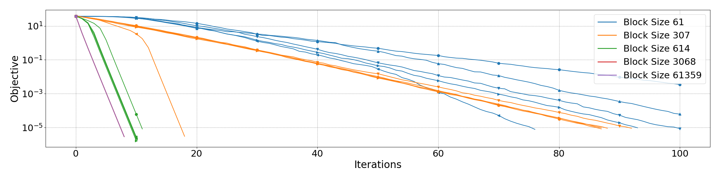
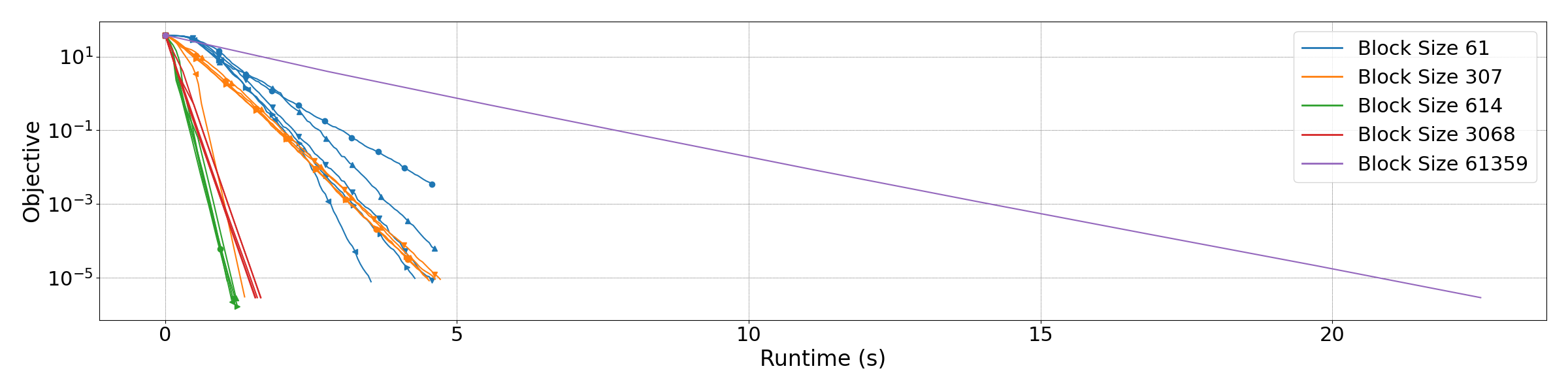
Figure 1: R-SGN on the chemotherapy dataset

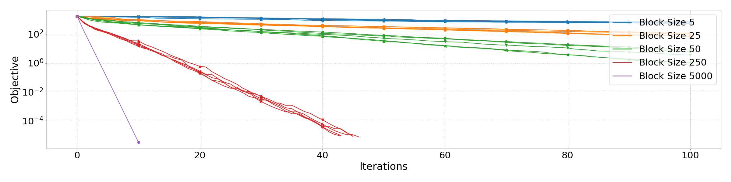
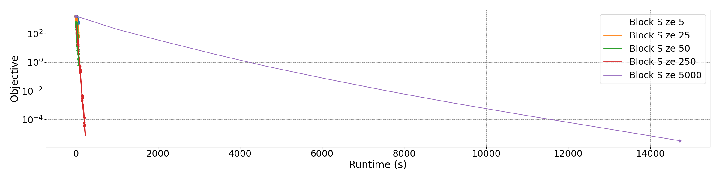
Figure 2: R-SGN on the gisette dataset

We first test on the chemotherapy and gisette datasets from OpenML (Vanschoren et al., 2013) for $100$ iterations with $\lambda=10^{-10}$, using block sizes of 0.1%, 0.5%, 1%, 5% and 100% of the original for the $61,359$ dimensional chemotherapy dataset and the $5,000$ dimensional gisette dataset; in a similar testing setup to Gower et al. (2019). As R-SGN is randomised, we perform five runs of the algorithm for each block size starting at $x_{0}=0$. We terminate once the objective $f(x_{k})$ goes below $10^{-5}$ and plot $f(x_{k})$ against iterations and runtime in each Figure. On the chemotherapy dataset, we see from Figure 1 that we are able to get comparable performance to full GN ($d=61,359$ in purple) using only $1\%$ of the original block size ($l=614$ in green) at $1/20$th of the runtime. For the gisette dataset, we see from Figure 2 that similarly, we are able to get good performance compared to GN ($d=5,000$ in purple) using $5\%$ of the original block size ($l=250$ in red) at $1/60$th of the runtime.

We next test on the artif and oscigrne nonlinear least-squares problems from the CUTEst collection (Gould et al., 2015) with dimension $5,000$ and $10,000$ respectively in both $n$ and $d$. As before we run R-SGN five times for each problem for $100$ iterations from the given starting points for each problem, with block sizes of 1%, 5%, 10%, 50% and 100% of the original. As we can see from the results in Figure 3 and Figure 4, R-SGN does not perform as well as on the logistic regression problems, due possibly to the increased difficulty/nonlinearity of these problems. However, it is still able to reach low accuracy solutions reasonably well, achieving a reduction of several orders of magnitude in the objective after just one second for both problems at $50\%$ block size (plotted in red). The CUTEst examples show that more sophisticated approaches may be needed to tackle general nonlinear least-squares problems; for example instead of keeping the block size fixed at $l$, we may consider increasing $l$ over iterations, a topic of future investigation.

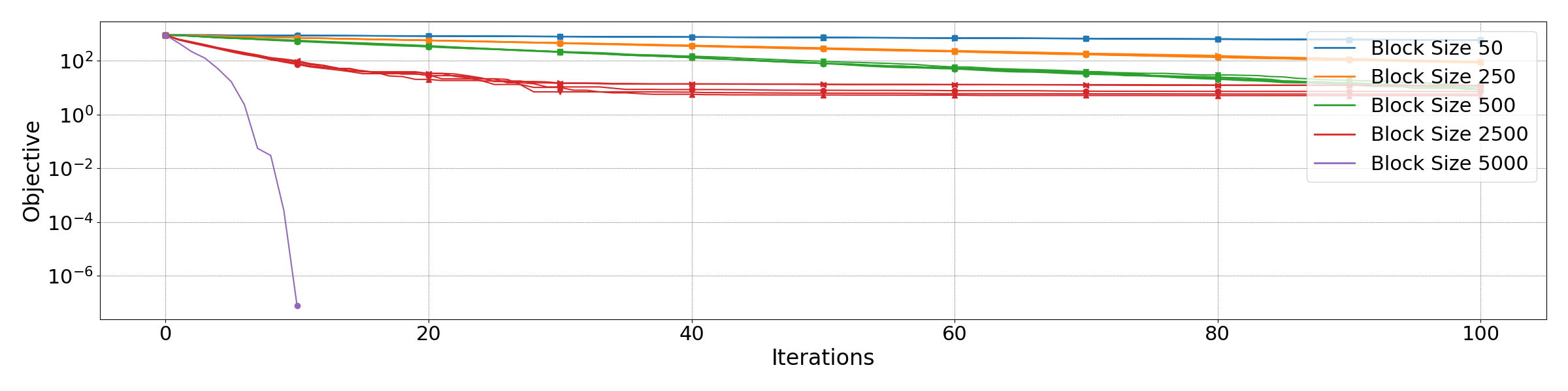
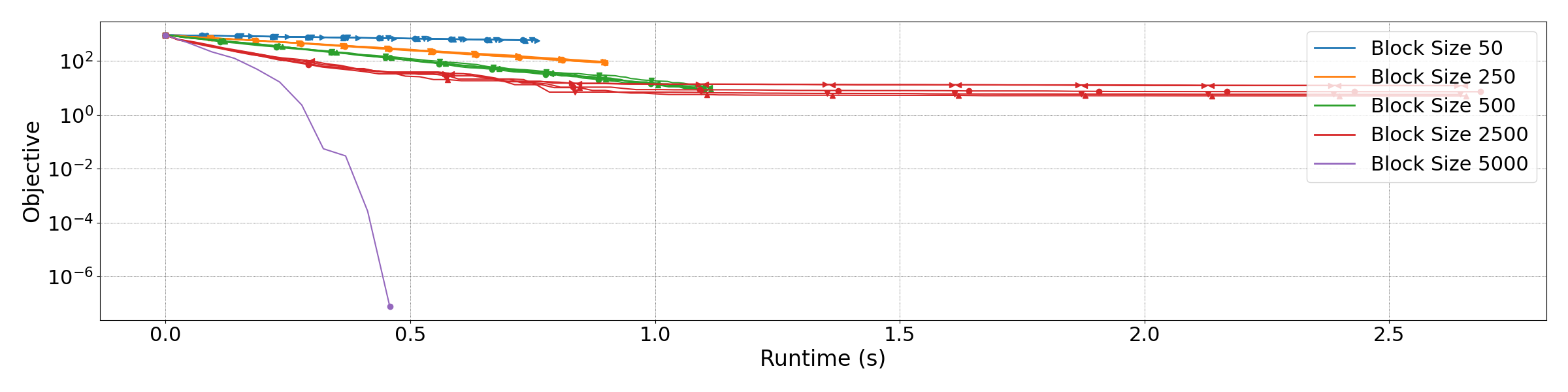
Figure 3: R-SGN on the artif dataset

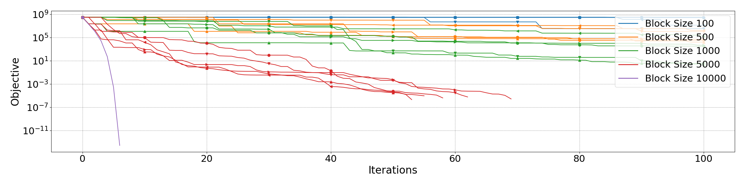
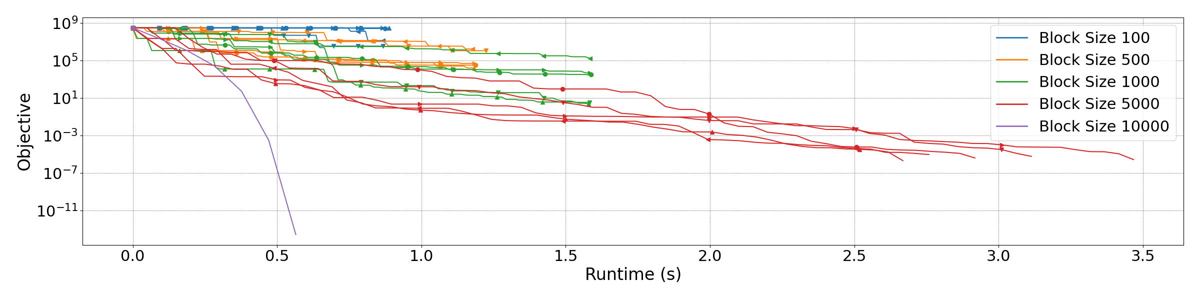
Figure 4: R-SGN on the oscigrne dataset

6 Conclusions

We have presented an optimization algorithm for solving nonlinear least-squares problems that uses a sketched Gauss-Newton approximation to the objective’s second derivatives, in a randomised subspace of the full space. A global rate of convergence, with high probability, is presented. We have demonstrated promising numerical results on logistic regression problems and nonlinear CUTEst test problems.

References

- Cartis & Scheinberg (2018) Cartis, C. and Scheinberg, K. Global convergence rate analysis of unconstrained optimization methods based on probabilistic models. Mathematical Programming, 169(2):337–375, 2018.
- Cartis et al. (2012) Cartis, C., Gould, N. I., and Toint, P. L. How much patience do you have? A worst-case perspective on smooth nonconvex optimization. Optima. Mathematical Optimization Society Newsletter, (88):1–10, 2012.
- Cohen et al. (2018) Cohen, M. B., Jayram, T., and Nelson, J. Simple analyses of the sparse Johnson-Lindenstrauss transform. 2018.
- Conn et al. (2000) Conn, A. R., Gould, N. I., and Toint, P. L. Trust region methods. SIAM, 2000.
- Dasgupta & Gupta (2003) Dasgupta, S. and Gupta, A. An elementary proof of a theorem of Johnson and Lindenstrauss. Random Structures & Algorithms, 22(1):60–65, 2003.
- Doikov & Richtárik (2018) Doikov, N. and Richtárik, P. Randomized block cubic Newton method. In International Conference on Machine Learning, pp. 1290–1298, 2018.
- Facchinei et al. (2015) Facchinei, F., Scutari, G., and Sagratella, S. Parallel selective algorithms for nonconvex big data optimization. IEEE Transactions on Signal Processing, 63(7):1874–1889, 2015.
- Gould et al. (2015) Gould, N. I., Orban, D., and Toint, P. L. CUTEst: a constrained and unconstrained testing environment with safe threads for mathematical optimization. Computational Optimization and Applications, 60(3):545–557, 2015.
- Gower et al. (2019) Gower, R., Koralev, D., Lieder, F., and Richtárik, P. RSN: randomized subspace Newton. In Advances in Neural Information Processing Systems, pp. 614–623, 2019.
- Gratton et al. (2007) Gratton, S., Lawless, A. S., and Nichols, N. K. Approximate Gauss–Newton methods for nonlinear least squares problems. SIAM Journal on Optimization, 18(1):106–132, 2007.
- Gratton et al. (2018) Gratton, S., Royer, C. W., Vicente, L. N., and Zhang, Z. Complexity and global rates of trust-region methods based on probabilistic models. IMA Journal of Numerical Analysis, 38(3):1579–1597, 2018.
- Kane & Nelson (2014) Kane, D. M. and Nelson, J. Sparser Johnson-Lindenstrauss transforms. Journal of the ACM, 61(1):1–23, 2014.
- Lu & Xiao (2017) Lu, Z. and Xiao, L. A randomized nonmonotone block proximal gradient method for a class of structured nonlinear programming. SIAM Journal on Numerical Analysis, 55(6):2930–2955, 2017.
- Luo et al. (2016) Luo, H., Agarwal, A., Cesa-Bianchi, N., and Langford, J. Efficient second order online learning by sketching. In Advances in Neural Information Processing Systems, pp. 902–910, 2016.
- Nocedal & Wright (2006) Nocedal, J. and Wright, S. Numerical optimization. Springer, 2006.
- Pilanci & Wainwright (2017) Pilanci, M. and Wainwright, M. J. Newton sketch: a near linear-time optimization algorithm with linear-quadratic convergence. SIAM Journal on Optimization, 27(1):205–245, 2017.
- Qu et al. (2016) Qu, Z., Richtárik, P., Takác, M., and Fercoq, O. SDNA: stochastic dual Newton ascent for empirical risk minimization. In International Conference on Machine Learning, pp. 1823–1832, 2016.
- Richtárik & Takáč (2014) Richtárik, P. and Takáč, M. Iteration complexity of randomized block-coordinate descent methods for minimizing a composite function. Mathematical Programming, 144(1-2):1–38, 2014.
- Rudelson & Vershynin (2010) Rudelson, M. and Vershynin, R. Non-asymptotic theory of random matrices: extreme singular values. In Proceedings of the International Congress of Mathematicians 2010, pp. 1576–1602. World Scientific, 2010.
- Tett et al. (2017) Tett, S. F., Yamazaki, K., Mineter, M. J., Cartis, C., and Eizenberg, N. Calibrating climate models using inverse methods: case studies with HadAM3, HadAM3P and HadCM3. Geoscientific Model Development, 10, 2017.
- Vanschoren et al. (2013) Vanschoren, J., van Rijn, J. N., Bischl, B., and Torgo, L. OpenML: networked science in machine learning. SIGKDD Explorations, 15(2):49–60, 2013.
- Woodruff (2014) Woodruff, D. P. Sketching as a tool for numerical linear algebra. arXiv preprint arXiv:1411.4357, 2014.