Essence of independence:
Hodge theory of matroids since June Huh
Abstract.
Matroids are combinatorial abstractions of independence, a ubiquitous notion that pervades many branches of mathematics. June Huh and his collaborators recently made spectacular breakthroughs by developing a Hodge theory of matroids that resolved several long-standing conjectures in matroid theory. We survey the main results in this development and ideas behind them.
2020 Mathematics Subject Classification:
05B35, 05E14, 14F43, 14C171. Introduction
The notion of “independence” resides everywhere, for example in graphs, vector configurations, field extensions, hyperplane arrangements, matchings, and discrete optimizations. Matroid theory captures the combinatorial essence of “independence” shared in these structures. For example, let us consider the following graph with edges labelled and the set of vectors .
|
We observe a common combinatorial structure: a subset of edges in is acyclic if and only if the corresponding subset of vectors is linearly independent. This combinatorial structure is encoded as a matroid, introduced by Whitney [Whi32].
Definition 1.1.
A matroid consists of a finite set , called its ground set, and a nonempty collection of subsets of , called the independent sets of , such that
-
if and , then , and
-
if and , then there exists an element such that .
The definition implies that every maximal independent set of has the same cardinality , which we call the rank of .
Graphs and vector spaces give prototypical examples of matroids:
-
•
When is identified with the set of edges of a finite graph , setting
defines a matroid . Matroids arising in this way are called graphical matroids.
-
•
When is identified with a finite set of vectors spanning a vector space , setting
defines a matroid . Matroids arising in this way are called realizable matroids.
We see that the graph and the set of vectors in Figure 1 define the same matroid.
1.1. Combinatorial sequences from a matroid
Several long-standing conjectures in matroid theory, recently resolved by June Huh and his collaborators, concern the behavior of sequences of invariants of a matroid. For a sequence of nonnegative real numbers, we say that it
-
•
is unimodal if there exists such that
-
•
is log-concave if for all ,
-
•
has no internal zeros if implies for all , and
-
•
is top-heavy if for all where is the largest index such that .
Note that a log-concave sequence is unimodal if and only if it has no internal zeroes. For a survey of unimodality and log-concavity in combinatorics, see [Sta89, Bre94].
We consider the following sequences of invariants of a rank matroid . For some of them, we describe them only for a graphical or a realizable matroid, postponing their descriptions for arbitrary matroids to Section 2.
-
(a)
For , let be the number of independent sets of of cardinality . In other words, the sequence is the -vector of the simplicial complex whose faces are the independent sets of .
-
(b)
We may also consider the -vector. That is, for , let be defined by the identity , where is as in (a).
-
(c)
Suppose is the graphical matroid of a finite connected nontrivial graph . The chromatic polynomial of is defined as
where a coloring of the vertices is proper if no edge has both vertices the same color. It is polynomial in of degree , and is always divisible by . Let be the absolute values of the coefficients of , starting from the highest degree term.
-
(d)
Continuing the assumption that is the graphical matroid of , we define as the absolute values of the coefficients of .
-
(e)
Suppose is the realizable matroid of a set of vectors spanning a vector space . Let be a sequence defined by setting for each ,
We leave it as an exercise to check that for the matroid associated to the graph or the vector configuration in Figure 1, we have:
| , | , |
| , | , |
| . |
Notice in this example that every sequence is unimodal, log-concave, and top-heavy. Several conjectures from the 70’s posited that these sequences are unimodal, log-concave, or top-heavy for an arbitrary matroid. We describe these conjectures and their history more fully in Section 2.2.
1.2. An approach from algebraic geometry
After decades of little progress, a breakthrough occurred when many of these conjectures were resolved for realizable matroids using algebraic geometry: Huh and Katz [Huh12, HK12] showed that the sequence (c) is log-concave (with no internal zeros), Huh [Huh15] showed that (d) is log-concave (with no internal zeros), and Huh and Wang [HW17] showed that (e) is top-heavy. These developments were particularly significant in light of the following phenomena in matroid theory:
The geometry of realizable matroids often inspires purely combinatorial constructions for all matroids. Certain geometric properties, a priori applicable only to realizable matroids, persist to all matroids through these purely combinatorial constructions. This is surprising because almost all matroids are not realizable [Nel18], but such a creative tension between geometry and combinatorics is a recurring theme in matroid theory.
A recent spectacular example of this phenomenon is the development of the Hodge theory of matroids by June Huh and his collaborators [AHK18, ADH22, BHM+22, BHM+], which successfully resolved conjectures about log-concavity or top-heaviness of the sequences (a),…,(e) for arbitrary (not necessarily realizable) matroids. They established that matroids satisfy combinatorial analogues of certain Hodge-theoretic properties in algebraic geometry, known sometimes as the “Kähler package”:
Definition 1.2.
Let be a finite-dimensional graded real vector space with a symmetric bilinear form , and let be a convex subset of graded linear operators satisfying for all . The triple is said to satisfy the Kähler package if the following three properties hold for all nonnegative integers :
-
(PD)
The pairing is non-degenerate (Poincaré duality).
-
(HL)
For any , the linear map
is an isomorphism (hard Lefschetz property in degree ).
-
(HR)
For any , the symmetric bilinear pairing
is positive definite when restricted to the kernel of the map given by (Hodge-Riemann relations in degree ).
Classical Hodge theory tells us that these properties are satisfied when is the cohomology ring of real -forms on a complex projective manifold, is the Poincaré duality pairing, and consists of multiplication by ample divisor classes (see [Huy05] or [Voi02]).
The geometry behind realizable matroids led to purely combinatorial constructions for various “cohomologies” of a matroid. These constructions include the Chow ring of a matroid [FY04, AHK18], the conormal Chow ring of a matroid [ADH22], and the intersection cohomology of a matroid [BHM+]. For a matroid realizable over , all three satisfy the Kähler package due to classical algebraic geometry. The incredible result of June Huh and his collaborators—Karim Adiprasito, Federico Ardila, Tom Braden, Graham Denham, Eric Katz, Jacob Matherne, Nick Proudfoot, Botong Wang—is that the Kähler package continues to hold for these “cohomologies” of a matroid even when the matroid is not realizable.
We survey this remarkable development in matroid theory and its connection to algebraic geometry in four parts. In Section 2, we give a brief introduction to matroids, and describe the long-standing conjectures resolved by the Hodge theory of matroids. In Section 3, we explain how the conjectures in the case of realizable matroids were resolved using algebraic geometry. In Section 4, we discuss the Kähler package for Chow rings of fans and matroids, and how the validity of (HR) implies the conjectures about log-concavity. In Section 5, we discuss the intersection cohomology of a matroid, and explain its implication to top-heaviness.
Several interesting topics had to be omitted, even though they are closely related to the topics discussed here. A partial list includes the following:
- •
- •
- •
We hope that this survey will spark the reader’s general interest in this active field of the study of matroids from an algebro-geometric perspective.
Notation.
Throughout, let be a finite set of cardinality . For a subset , we denote by the sum of standard basis vectors in , where the field will be clear in context. An algebraic variety is reduced and irreducible (over an algebraically closed field).
Acknowledgements
The author thanks June Huh for helpful conversations, and Matt Baker, Andrew Berget, Tom Braden, Eric Katz, Matt Larson, and Lauren Williams for helpful suggestions and comments on a preliminary draft of this article.
2. Background in matroid theory
Here we give a minimal introduction to matroids. In addition to standard references on matroids such as [Wel76, Oxl11], we point to [Ard22, Bak18, Huh18, Kat16] for surveys tailored towards studying matroids from an algebro-geometric viewpoint.
2.1. Constructions
Since subsets of independent sets are independent, we may specify a matroid by its maximal independent sets, called the bases of the matroid.
Example 2.1.
For an integer , the uniform matroid of rank on is the matroid whose bases are all subsets of cardinality . When , we say that is the Boolean matroid on . The Boolean matroid , i.e. when so , is called the trivial matroid. Any uniform matroid is realizable over any infinite field as a general collection of vectors in .
Example 2.2.
We may visualize a collection of vectors in a 4-dimensional vector space as a collection of points in the projective 3-space . For example, the 5 column vectors of the matrix
![[Uncaptioned image]](/html/2211.05724/assets/x2.png)
|
can be visualized as the purple points, four of which lie in a common projective plane. The bases of this matroid are .
We define the dual matroid of a matroid on ground set by declaring
For example, we have . For the matroid in 2.2, its dual has the set of bases . Many notions in matroid theory come in pairs via matroid duality. For instance, an element is a loop of if it is in no bases, and is a coloop if it is in every basis of . The matroid in 2.2 has no loops and has a coloop 5, or equivalently, its dual matroid has no coloops and has a loop 5.
Another useful way of describing a matroid is by its rank function. For a matroid , its rank function is defined by
In particular, an independent set of a matroid is a subset whose rank equals its cardinality . That is, independent sets are the minimal subsets of with respect to a given rank. Considering the maximal subsets leads to the notion of flats of a matroid.
Definition 2.3.
A flat of a matroid on is a subset of that is maximal for its rank. That is, a subset is a flat of if .
The set of flats of a matroid forms a poset under inclusion. This poset is a lattice with meet and join defined by
For example, the lattice of flats of the matroid in 2.2 is
Exercise 2.4.
-
(1)
Show that every subset is contained in a unique flat of the same rank. In particular, the join of flats is well-defined.
-
(2)
How can one recover the bases of a matroid from the lattice of its flats?
-
(3)
Compute the lattice of flats of the matroid of the graph in Figure 1.
We record some linear algebraic interpretations of the notions introduced for a matroid realized by a set of vectors spanning a vector space :
-
•
The bases of are subsets such that is a basis of .
-
•
An element is a loop if and only if .
-
•
We have for any subset .
-
•
The flats of are subsets such that for some linear subspace . That is, the flats correspond to the different spans of subsets of the vectors.
Per the last bullet point, we now define the sequence (e) for arbitrary matroids.
Definition 2.5.
For a matroid of rank , the Whitney numbers of the second kind are defined by
Exercise 2.6.
Show that if is the graphical matroid of the complete graph on vertices, then its flats of rank correspond to partitions of into (nonempty) parts. In particular, the numbers in this case are known as the Stirling numbers of the second kind.
Matroid duality also admits a linear algebraic interpretation, given in the next exercise.
Exercise 2.7.
Let be the map given by , and let be its kernel. The short exact sequence dualizes to . Show that the surjection realizes the dual matroid .
An important pair of operations for forming new matroids from a given matroid is the restriction and contraction.
Definition 2.8.
For a matroid on ground set , and a subset , we define two matroids and on ground sets and , respectively, by specifying their rank functions:
| for all . | |||
The matroid is called the restriction of to , and the matroid is called the contraction of by . The deletion of by is the restriction .
These operations behave particularly well for a flat of a matroid :
-
•
The set of flats of is .
-
•
The set of flats of is .
These operations have a graphical and linear algebraic interpretations as well: For the graphical matroid of a graph , deletion corresponds to deleting the corresponding edges, and contraction corresponds to contracting the corresponding edges. When a matroid is realized by a set of vectors , the restriction is realized by the subset of vectors . The contraction is realized by the images of the vectors under the quotient by the span of .
Exercise 2.9.
Show that deletion and contraction are dual notions, that is, we have .
2.2. Invariants
Introduced for graphs by Tutte [Tut67] and extended to matroids by Crapo [Cra69], the Tutte polynomial is among the most famous invariants of a matroid. For the proofs of the statements here, as well as a fuller treatment of Tutte polynomials, see [BO92].
Definition 2.10.
Tutte polynomial of a matroid of rank on ground set is the bivariate polynomial defined by
The Tutte polynomial is the universal deletion-contraction invariant:
Theorem 2.11.
The Tutte polynomial can be defined recursively by
with . If is an invariant of matroids with values in a (commutative unital) ring such that and there exists satisfying
for all matroids and an element . Then, we have
The theorem implies the following basic properties of the Tutte polynomial:
-
•
The Tutte polynomial of a matroid has nonnegative coefficients.
-
•
The constant term of is zero unless is the trivial matroid.
-
•
For the dual matroid , we have .
Univariate specializations of the Tutte polynomial lead to many interesting combinatorial sequences. For example, we deduce from the definition that for a matroid of rank ,
where we recall from (a) that is the number of independent sets of of cardinality . Consequently, we have that the sequence of (b) is given by
Another important specialization is the characteristic polynomial of a matroid of rank , defined as
The basic properties of the Tutte polynomial listed above imply that the coefficients of have alternating signs, and that is divisible by unless is a trivial matroid. Thus, one often divides out to define the reduced characteristic polynomial . It follows from 2.11 that if has a loop.
The characteristic polynomial of a graphical matroid essentially equals the chromatic polynomial of the graph in the following way.
Exercise 2.12.
Show that if is the graphical matroid of a finite graph , and has connected components, then . (Hint: Appeal to 2.11 by showing that both satisfy an identical deletion-contraction relation).
We may now define the sequences (c) and (d), which we previously only defined for graphical matroids, for arbitrary nontrivial matroids: they are the coefficients of and , respectively.
Summarizing, we have the following sequences for a matroid of rank .
-
(a)
The coefficients of .
-
(b)
The coefficients of .
-
(c)
The coefficients of .
-
(d)
The coefficients of .
-
(e)
The Whitney numbers of the second kind of .
Theorem 2.13.
[AHK18, ADH22, BHM+] Let be a matroid of rank .
-
(a)
The sequence is unimodal, log-concave, and top-heavy.
-
(b)
The sequence is unimodal, log-concave, and top-heavy.
-
(c)
The sequence is unimodal, log-concave, and top-heavy.
-
(d)
The sequence is unimodal, log-concave, and top-heavy.
-
(e)
The sequence satisfies for all . In particular, it is top-heavy.
The statements of the theorem were long-standing conjectures in matroid theory. The unimodality and log-concavity conjectures are due to: Welsh [Wel71] and Mason [Mas72] for (a), Dawson [Daw84] for (b), Read [Rea68] and Hoggar [Hog74] for (c) of graphical matroids, Heron [Her72], Rota [Rot71], and Welsh [Wel76] for (c), and Brylawski [Bry82] for (d). Hibi [Hib92] and Swartz [Swa03] posed the top-heaviness of (b) and (d) (respectively).111A slightly different terminology of flawless-ness appears in [Hib92] and related works [Hib89, JKL18]. A nonnegative sequence is flawless if it is top-heavy and additionally satisfies , where is the largest index such that . Note that unimodal and top-heavy sequences are flawless. Dowling and Wilson [DW74, DW75] conjectured the top-heaviness of (e), generalizing a theorem of de Bruijn and Erdös [dBE48] on point-line incidences in projective planes. There are two notable conjectures on (e) that remain open: Rota [Rot71] conjectured its unimodality, and Mason [Mas72] its log-concavity.
Remark 2.14.
One may ask if there is a log-concavity statement for the whole Tutte polynomial of a matroid that explains the log-concavity of the four specializations in 2.13. This was achieved by Berget, Spink, Tseng, and the author [BEST23] who showed that the 4-variable transformation
of the Tutte polynomial of a matroid satisfies a multivariate version of log-concavity. We note that without such a transformation, the coefficients of can fail to be unimodal [Sch93].
In this survey, we will explain how the sequences (c) and (d) are shown to be log-concave with no internal zeros,222As observed by Lenz [Len13], a result of Brylawski [Bry77, Theorem 4.2] implies that the statements for (a) and (b) follow from those for (c) and (d). The top-heaviness of (c) and (d) follows from their unimodality due to [JKL18, Theorem 1.2]. and how the sequence (e) is shown to be top-heavy. Since if has a loop, and deleting loops of a matroid does not change the lattice of its flats, we assume the following:
Assumption. From now on, a matroid is loopless unless specified otherwise.
3. The realizable case
We explain how the statements in 2.13 can be deduced using algebraic geometry when the matroid in question is realizable. We assume familiarity with algebraic geometry; those who prefer purely combinatorial treatments may skip this section. For simplicity, we consider matroids realizable over . For other fields, one can run nearly identical arguments using the Chow cohomology ring [Ful98] or the -adic (intersection) cohomology in place of singular (intersection) cohomology with rational coefficients.
Throughout this section, let be a (nontrivial) matroid of rank realized by a set of vectors spanning a vector space . The corresponding surjection dualizes to give an -dimensional linear subspace .
Notation. Let us denote to avoid repeated use of the superscript .
The set of independent sets of can then be described also as the collection
We will often projectivize and work with .
3.1. Hyperplane arrangements
We first discuss some structures of the matroid in terms of its realization as a subspace . For each let be the -th coordinate hyperplane of . Our assumption that is loopless implies that is not contained in any . We thus have a hyperplane arrangement on consisting of the hyperplanes . Dualizing the correspondence between the flats of and the spans of subsets of the vectors , we obtain a correspondence
Note that the correspondence is order-reversing, and in particular, a flat of rank maps to the linear subspace of dimension .
Example 3.1.
The columns of the matrix below realizes the matroid . Equivalently, the embedded subspace , where is the row-span of the matrix, realizes the matroid .
![[Uncaptioned image]](/html/2211.05724/assets/x3.png) |
Next to the matrix, we have depicted the lattice of flats of and the projectivization of the hyperplane arrangement in .
We denote the complement of the hyperplane arrangement by
Exercise 3.2.
Suppose is not a coloop, and let be the smallest flat containing . Show that the subspace is a realization of the contraction , and that the hyperplane arrangement complement is a realization of the deletion . What happens when is a coloop?
The geometric study of (complements of) hyperplane arrangements and its interaction with matroid theory is a rich and on-going research field; some references include [OT92, Dim17]. Here, we only note the following classical fact [OS80], which states that the characteristic polynomial records the dimensions of the cohomologies of the arrangement complement.
Theorem 3.3.
Let realize a matroid of rank . Then, we have
or equivalently, by applying the Künnuth formula to ,
3.2. Log-concavity via intersection degrees
We now explain how the log-concavity of the sequences (c) and (d) can be shown using algebraic geometry. We start by describing a general strategy for log-concavity.
Let be a smooth projective -variety of dimension . When considered as a -dimensional real compact manifold, Poincaré duality for the cohomology ring provides the isomorphism , called the degree map. Recall that a divisor on is ample (resp. semi-ample) if the line bundle is very ample (resp. globally generated) for some integer . The general strategy arises from the following Khovanskii-Teissier inequalities (see [Laz04a, Section 1.6] for a history and a fuller treatment).
Proposition 3.4.
Let be the cohomology classes of two semi-ample (or more generally, nef) divisors on a smooth projective -variety of dimension . Then,
is log-concave with no internal zeros.
Sketch of the proof.
By continuity, one can assume to be ample, and then one reduces to the case of surfaces via the Bertini theorem. Then, one of the equivalent forms of the Hodge index theorem for surfaces [Har77, Exercise V.1.9] exactly yields the desired log-concavity. We note that the Hodge index theorem for surfaces stated as [Har77, Theorem V.1.9] is exactly the validity of the Hodge-Riemann relations for surfaces. ∎
Thus, starting from the realization , one may seek a smooth projective -variety equipped with two semi-ample divisor classes such that their intersection degrees yield the appropriate combinatorial sequence. We explain how this is done for the sequences (c) and (d).
3.2.1. Log-concavity of (c)
We show the slightly stronger statement that the closely related sequence defined by
is log-concave with no internal zeros. 3.3 states that this sequence is exactly the Betti numbers of the arrangement complement . The sought-after projective variety is the wonderful compactification of a hyperplane arrangement complement introduced in [DCP95].
Definition 3.5.
The wonderful compactification is the variety obtained by blowing-up at all the points , then by blowing-up all strict transforms of the lines , and so forth. Let be the blow-down map.
By construction is isomorphism on the open loci . The boundary is a simple-normal-crossing divisor on [DCP95]. For the sought-after divisor classes on , the wonderful compactification for the Boolean matroid plays a special role.
When , that is, when , the wonderful compactification is known as the permutohedral variety . Explicitly, it is obtained from by blowing-up all coordinate points of , then blowing-up all strict transforms of coordinate lines of , and so forth. Let be the blow-down map. Blowing-down the exceptional divisors in a “reverse manner” (see [Huh18] for a detailed description via toric geometry), one obtains a different blow-down map . The resulting birational transformation is the Cremona transformation given by in the projective coordinates.
Returning to the case where is not necessarily Boolean, we note the following: Because the arrangement on is the restriction to of the coordinate hyperplane arrangement on , the universal property of blow-ups implies that is the strict transform of under the blow-up . Summarizing, we have a commuting diagram:
| () |
Let be the hyperplane class of , and define divisor classes and on to be the restrictions of and , respectively. Huh–Katz [HK12] showed that
Since and are both hyperplane class pullbacks, they are globally-generated, so 3.4 implies the desired log-concavity.
How might one think to do this, at least in hindsight? Two key steps are as follows.
-
(1)
The commuting diagram ( ‣ 3.2.1) shows that is also the pullback to of the hyperplane class in , so we may loosely interpret multiplication by as restriction to a general hyperplane in . As a linear subvariety , this hyperplane is again a realization of a matroid, known as the truncation matroid of . With well-known properties of characteristic polynomials [Zas87], it is straightforward to verify that is obtained from by erasing the constant term and then dividing by . That is, the sequence for is obtained from that of by simply removing the last entry.
-
(2)
With the previous step, we now only need compare with the constant term . Let be the closure of the image of under the Cremona transformation, often known as the reciprocal linear space. By the construction of , the degree of as a subvariety of equals . On the other hand, the degree of also equals . This last key fact was proven in several contexts [Ter02, PS06, Huh12, HK12]. A topological approach in [Huh12] is as follows: A result of Dimca and Papadima [DP03] from (complex) Morse theory related the Euler characteristic of a hypersurface complement to the degree of the gradient map. The hypersurface is the coordinate hyperplane arrangement that restricts to the hyperplane arrangement on , and the gradient map of is exactly the Cremona map. Combining these facts with 3.3, one can deduce .
Exercise 3.6.
Let be as in 3.1. Verify that , and verify that is a cubic surface known as the Cayley nodal cubic. This cubic surface has four singular points, with a line through each pair of points; explain where these come from in terms of the wonderful compactification . (Bonus: This cubic surface has three more lines, for the total of nine; where do they come from?)
3.2.2. Log-concavity of (d)
The sought-after projective variety is the variety of critical points , formally introduced in [CDFV11] but implicit in previous works related to Varchenko’s problem on critical points of master functions on an affine hyperplane arrangement [Var95]. Here, in order to build upon our previous discussion in Section 3.2.1, we follow [BEST23, Section 8] to describe a smooth birational model of in terms of the wonderful compactification , although it differs slightly from the original description in [Huh15].
Consider the embedding in the diagram ( ‣ 3.2.1). Let be the normal bundle, and let be the projectivization333Our convention for the projectivization of a vector bundle on a variety is that , which agrees with [EH16] but is the opposite of [Har77, Laz04b]. of the conormal bundle with the projection map . Recall the blow-down map .
The sought-after divisor classes on are as follows. Let be the pullback of the hyperplane class in via the composition . Let be the first Chern class of the line bundle from the construction of as a projectivization of a vector bundle, which turns out to be semi-ample. One can then translate [DGS12, Theorem 1.1] to the statement that
3.4 now implies the desired log-concavity.
How might one think to do this, at least in hindsight? For the original formulation of , maximum likelihood problems in algebraic statistics provided a motivation; see [Huh13, HS14]. For the related construction here, we highlight some key steps. In either cases, one uses properties of log-tangent bundles and their characteristic classes; see [Alu05] for an introduction to these tools.
-
(1)
By 3.3, the constant term equals
the signed Euler characteristic of . Euler characteristics satisfy the “scissors relation” that for a closed embedding of -varieties. More generally, Chern-Schwartz-MacPherson (CSM) classes [Mac74] of -varieties are homological objects that respect such scissors relation. One then uses 3.2 to show that the degrees of the CSM classes of satisfy the same deletion-contraction relation satisfied by the coefficients of , so that 2.11 implies that they are the same.
-
(2)
Having related the CSM classes to , we now relate powers of with the CSM classes of . The varieties and have simple-normal-crossing boundaries and . Under the embedding , one can show that scheme-theoretically. Consequently, one has a short exact sequence (see for instance [EHL, Section 9])
Because is a toric variety with the dense open torus , the log-tangent bundle is trivial [CLS11, Chapter 8]. Thus, the normal bundle is globally-generated so that is semi-ample. Moreover, the Segre classes of , which are given by powers of , equal the Chern classes of , which are the CSM classes of the complement [Alu99].
3.3. The top-heaviness via intersection cohomology
We start with a general strategy for establishing top-heaviness, which first appeared in [BE09] to establish top-heaviness for Bruhat intervals. Suppose we have a (not necessarily smooth) projective -variety with an affine stratification: There is a finite collection of locally closed subvarieties of , called the strata, such that is the disjoint union of , the closure of any strata is again a union of strata, and each strata is isomorphic to for some .
Theorem 3.7.
[BE09, Theorem 3.1] For , let be the number of strata of dimension . Then, we have for all .
Sketch of the proof.
Let us assume we have shown that . If were smooth, the hard Lefschetz theorem implies that is in fact unimodal and symmetric, so we would be done. Since may not be smooth, we need to consider the intersection cohomology , for which the hard Lefschetz theorem still holds [GM83, BBD82]. There is a natural graded map , fitting into a commutative diagram
for any ample line bundle on , where the injectivity of the right vertical map follows from the validity of the hard Lefschetz property for intersection cohomology. Thus, if is injective, then the left vertical map is necessarily injective, so we can conclude the desired .
Björner and Ekedahl [BE09] used 3.7 on Schubert varieties of a generalized flag variety to deduce top-heaviness for Bruhat intervals of a finite crystallographic Coxeter group. In our case, for a realization of a matroid , we consider its matroid Schubert variety defined as
where via the identification . Note that the identification induces an affine stratification of with strata . One shows that this stratification restricts to give an affine stratification of by using the computation of (the Gröbner basis for) the defining ideal of given by Ardila and Boocher [AB16].
Theorem 3.8.
Exercise 3.9.
Verify 3.8 for a realization of the uniform matroid .
For Schubert varieties in generalized flag varieties, their intersection cohomology is closely related to Kazhdan-Lusztig theory. The terminology “matroid Schubert variety” was chosen because of the analogous relation between the intersection cohomology and Kazhdan-Lusztig theory of matroid developed in [EPW16, PXY18].
4. Tropical Hodge theory
We will begin by explaining how polyhedral fans and matroids give rise to “cohomology” rings. We then discuss two fundamental theorems for these “cohomology” rings concerning the validity of the Kähler package (1.2). We then explain how the log-concavity statements for arbitrary matroids can be deduced from these fundamental theorems. We will assume some familiarity with the basics of polyhedral geometry. For a brief introduction see [Ful93, Chapter 1.2], and see [Zie95] for a fuller treatment.
4.1. Chow rings of fans and matroids
Let be a lattice, i.e. a finitely generated free abelian group . Let denote its dual lattice. We write . Recall that a fan in is rational if each ray in equals for some , simplicial if every -dimensional cone in is generated by rays, and pure-dimensional if every maximal cone has the same dimension. For each ray , let be the primitive ray generator, i.e. the element such that . Let denote the set of rays of . The support of is denoted . A fan in is complete if .
Assumption.
All fans we treat will be rational, simplicial, and pure-dimensional, but not necessarily complete.
Definition 4.1.
The Chow (cohomology) ring (with real coefficients) of a fan in is the graded -algebra
where and are the ideals
It is an exercise to show that the -th graded piece of is generated by square-free monomials of degree in the variables. In particular, for all greater than the dimension of , and is a finite-dimensional graded real vector space.
Exercise 4.2.
For two fans and , show that .
Borrowing language from algebraic geometry, let us call a linear combination of the variables a divisor and its image in its divisor class on . Because is simplicial, a divisor determines a piecewise-linear function on by assigning the value to each primitive ray generator .
Definition 4.3.
A divisor on a complete fan is ample if the piecewise-linear function is strictly-convex, i.e. for all not in the same cone of . It is nef if only the weak inequality is satisfied.
For a not necessarily complete fan , a divisor is ample (resp. nef) if is the restriction of the piecewise-linear function of an ample (resp. nef) divisor on a complete fan containing as a subfan. We denote by the convex set of the divisor classes of ample divisors on .444Technically, our definition of ample/nef divisors on non-complete fans differs from that of [ADH22], which makes our a subset of the one in [ADH22], but will suffice for our discussion. We often consider as a set of graded linear maps given by multiplication.
In terms of toric geometry, the ring is the Chow cohomology ring of the toric variety associated to the fan [Dan78, Bri96]. When is the normal fan of a simple polytope, the toric variety is a projective variety with mild (i.e. orbifold) singularities, whose ample cone is . Classical results in algebraic geometry then imply the validity of the Kähler package for the ring . Stanley used this to resolve McMullen’s -conjecture on the number of faces of a simple polytope [Sta80]. Afterwards, McMullen [McM93] gave a purely combinatorial proof of the Kähler package that works even for nonrational fans (with no associated toric variety in the background). In our case, the fans will not in general be complete, so a priori there is no reason to expect any validity of the Kähler package, since the associated toric varieties are not in general compact. The miraculous result is that certain fans from matroids turn out to enjoy the Kähler package.
For a matroid on of rank , we construct a fan introduced and studied in [Stu02, AK06, Spe08] as tropical geometric analogue of linear spaces. The fan will be in the real vector space over the lattice . For a subset , let us denote by the image of under the quotient map .
Definition 4.4.
The Bergman fan of a rank matroid is a pure -dimensional fan in consisting of the maximal cones , one for each maximal chain of nonempty proper flats of .
Example 4.5.
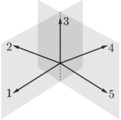
The Bergman fans of and are depicted below.
![[Uncaptioned image]](/html/2211.05724/assets/x4.png) |
![[Uncaptioned image]](/html/2211.05724/assets/x5.png)
|
Example 4.6.
For the Boolean matroid , note that the maximal cones of its Bergman fan correspond to permutations of the ground set . The fan is known as the permutohedral fan or as the braid arrangement, denoted . Note that by construction the Bergman fan of any matroid (on ground set ) is a subfan of . See [AA] for a survey of remarkable combinatorial properties of the permutohedral fan.
Definition 4.7.
The Chow ring of a matroid is the Chow ring of its Bergman fan. Explicitly, it is
where and are the ideals
Remark 4.8.
When has a realization , the wonderful compactification defined in Section 3.2.1 is the closure of inside the toric variety . The resulting pullback map of cohomologies is an isomorphism between the Chow ring of the toric variety of and the cohomology ring of [FY04, DCP95]. This “Chow equivalence” is informed by the theory of tropical compactifications [Tev07]; see [MS15, Chapter 6] for an introduction. While the Kähler package for the Chow ring in this realizable case thus follows from classical Hodge theory, [AHK18, Theorem 5.12] states that the existence of such Chow equivalence is equivalent to the realizability of the matroid.
We note another fan associated to a matroid whose Chow ring will be used for log-concavity statements.
Definition 4.9.
The conormal fan of a (loopless and coloopless) matroid is a fan in whose support equals the support of the product .
We omit the precise definition, which involves the intricate and interesting combinatorics of the bipermutohedron and biflags introduced in [ADH22]. See [ADH22, Section 2.8] for its origin story.
Remark 4.10.
Just as the Chow ring of a matroid is modeled after the wonderful compactification, the conormal Chow ring of a matroid is modeled after the geometry described in Section 3.2.2. For instance, 2.7 suggests how the product can serve as a polyhedral model of the projectivized conormal bundle .
4.2. Fundamental theorems of tropical Hodge theory
We now discuss two fundamental theorems concerning the Kähler package for Chow rings of not necessarily complete fans. To state them, we need a few more terminologies.
For a cone of a fan in , the star is a fan in whose cones are the images under the projection of the cones of containing . Geometrically, the toric variety of the star is the closure of the torus-orbit of corresponding to the cone .
Exercise 4.11.
-
(1)
The star of the Bergman fan at the ray corresponding to a nonempty proper flat is isomorphic to the product .
-
(2)
Show that the Chow ring of the star is isomorphic to the quotient ring .
A positive Minkowski weight on a (pure) -dimensional fan is a linear map such that for any maximal cone of . It defines a symmetric bilinear pairing by , which by abuse of notation we also denote .
Geometrically, Minkowski weights in general are fundamental objects in tropical intersection theory, serving the role of “Chow homology classes.” For their definition and properties, see [FS97, KP08] and [MS15, Chapter 6], as well as [AHK18, Section 5]. Fans arising in the context of tropical compactifications (4.8) provide many examples of positive Minkowski weights. For instance, the following can be deduced from what is known as the cover-partition property of flats.
Proposition 4.12.
[AHK18, Proposition 5.2] For a matroid of rank , the assignment for any maximal chain of nonempty proper flats of gives a well-defined linear map .
Similarly, the conormal fan of a matroid also has a natural positive Minkowski weight . The key notion for the statement of the two fundamental theorems is the notion of Lefschetz-ness of fans, introduced in [ADH22].
Definition 4.13.
A fan of dimension is said to be Lefschetz if the following are satisfied:
-
(1)
is spanned by a positive Minkowski weight .
-
(2)
The triple satisfies the Kähler package (1.2).
-
(3)
For any positive dimensional cone of , the star is Lefschetz.
We can now state the two fundamental theorems.
Theorem 4.14.
[AHK18, Theorem 1.4] The Bergman fan of a matroid is Lefschetz.
Theorem 4.15.
[ADH22, Theorem 1.6] Let and be fans in with the same support, and suppose and are nonempty. Then is Lefschetz if and only if is Lefschetz.
The product of two Lefschetz fans is again Lefschetz [AHK18, Section 7.2]. Combining this with the two theorems yields the following.
Corollary 4.16.
The conormal fan of the matroid is Lefschetz.
Exercise 4.17.
Let be a matroid of rank . Let for any . Note that is independent of the choice of due to the linear relations .
-
(1)
Show that for any flat of rank 2.
-
(2)
Show that for any element .
-
(3)
Show that for any element and a flat of rank 2.
-
(4)
Use these steps to establish the Kähler package for with .
Let us give a broad overview of the proofs of the two theorems. Both employ the following strategy for establishing the Kähler package for a graded -algebra of “dimension ” in the sense that . This general strategy and variations thereof appear in several previous works on the Kähler package across varied mathematical fields, such as the works of McMullen [McM93] on simple polytopes, Elias and Williamson [EW14] on Soergel bimodules, and [dCM09] on the topology of algebraic maps.
- (i)
-
(ii)
Next, one can set up an induction on the “dimension” as follows. In many situations, the quotient algebra for certain choices of is again in the family of graded -algebras that one is seeking to establish the Kähler package for. Here, denotes the annihilator . The key observation then is that
(see for instance [BES, Proposition 6.1.6]). Because the quotient has smaller “dimension”, i.e. its -th graded part is zero, one can now proceed by induction on .
-
(iii)
By the validity of (HL) from the inductive hypothesis, the validity of (HR) for any single element then implies (HR) for all . Thus, the last step is to finish the induction by establishing (HR) for a well-chosen . This is often the most intricate step.
Returning to the case of matroids, step (ii) is provided by 4.11, which showed that for a nonempty proper flat of . Hence, one can induct on the rank of the matroid. In the case of 4.15, step (ii) is essentially built into the definition that the stars of Lefschetz fans are Lefschetz, so that one can induct on the dimension of the fan.
In the original proof [AHK18] of 4.14, in order to carry out step (iii), Adiprasito, Huh, and Katz introduced the notion of “flips,” inspired by the proof of the Kähler package for simple polytopes by McMullen [McM93]. This process converts the Bergman fan of through a sequence of fans until it reaches a fan for which (HR) can be verified easily, and the process is set up such that the validity of (HR) for any one fan in the sequence implies (HR) for all fans in the sequence. Geometrically, one may interpret the process of flips as a combinatorial abstraction of the process of constructing the wonderful compactification as a sequence of blow-ups (3.5).
Afterwards, it was recognized that a key property of semi-small maps [dCM02] inspires a strategy that can greatly simplify step (iii). For a map of smooth projective varieties, the pullbacks to of ample divisors on generally fail (HL) and (HR) in the cohomology ring of , since the pullbacks are generally not ample on but only nef (i.e. is a limit of ample divisors). However, a characterizing property of a semi-small map is that the pullbacks still satisfy (HL) and (HR). This inspires the following approach: One can look for a map of graded algebras, behaving like a pullback along a semi-small map. If (HR) is known to hold for , say by induction, step (iii) would follow.
This insight allowed Braden, Huh, Matherne, Proudfoot, and Wang to give a considerably simplified proof of 4.14 in [BHM+22]. Using that the deletion of a matroid by a non-coloop element behaves like a semi-small map, they carry out step (iii) by an induction that reduces to the case of Boolean matroids. This insight on semi-small maps is also essential in the proof of 4.15 by Ardila, Denham, and Huh. A key step [ADH22, Theorem 5.9], building upon the works [Wło97, AKMW02], states that any two fans with the same support can be related by a sequence of edge stellar subdivisions, which are operations on fans that play the role of semi-small maps in toric geometry.
4.3. Applications of Hodge-Riemann relations in degree 1
The Kähler package gives rise to log-concave sequences in the following way.
Proposition 4.18.
Suppose is a Lefschetz fan of dimension with a positive Minkowski weight . Then, for any nef divisor classes and ,
is log-concave with no internal zeros.
Proof.
We may assume that are ample, and show that the sequence is strictly positive and log-concave, since a limit of such sequences is necessarily log-concave with no internal zeros. Strict positivity is then implied by Hodge-Riemann relations (HR) in degree 0. For log-concavity, (HR) in degree 1, with , implies that the symmetric bilinear pairing given by has at most one positive eigenvalue. This implies that the symmetric matrix
cannot be positive definite, but it also cannot be negative definite because all of its entries are positive. Hence, the determinant of the matrix is non-positive, or equivalently, . ∎
Returning to showing log-concavity for a matroid of rank , one now searches for appropriate divisor classes on the Bergman fan or the conormal fan . This step benefits heavily from the geometry of realizable matroids explained in Section 3.
The divisor classes for the log-concavity of the sequence (c) come from an involutive symmetry of the permutohedral fan (4.6). As , the minus map on gives an involution of . This equips with two distinguished coarsenings to a normal fan of a simplex: Let (resp. be ) be the fan whose rays are (resp. ) and whose cones are generated by any subsets of the rays with cardinality . The fan is a common refinement of both the fans and .
Let us fix an element , and let be the piecewise-linear function on given by and for all , which is clearly a convex (but not strictly-convex) function. Restricting this piecewise-linear function to , it defines a divisor on whose divisor class is denoted . Similarly, starting with the fan , we obtain a divisor class . Both and are nef, and independent of the choice of we fixed. Algebraically, we may take and for any choice of . We have the following.
Proposition 4.19.
Combining the proposition with 4.14 and 4.18, we obtain that the coefficients of are log-concave with no internal zeros, which implies the same property for the coefficients of , i.e. the log-concavity of the sequence (c). One can also consider other kinds of divisor classes on and their values under to study properties of matroids: See for instance [Eur20, BES, BST, DR22].
Remark 4.20.
In geometric terms, the toric variety of is the permutohedral variety defined in Section 3.2.1. That the fan coarsens to and gives the two blow-down maps , related by the Cremona transformation, which were described in ( ‣ 3.2.1). Thus, the divisor classes and here and the computations involving them agree with those described in Section 3.2.1.
For the sequence (d), recall that the conormal fan of a matroid is a fan in with support equal to the support of . Let
By pulling back the piecewise-linear function on along these two maps, we obtain two divisor classes and .
Proposition 4.21.
[ADH22, Theorem 1.2] With the notations as above, we have
Combining the proposition with 4.16 and 4.18, we conclude the log-concavity of the sequence (d). The proposition was proved via an intricate combinatorics of biflags in [ADH22] and the Chern-Schwartz-MacPherson classes of matroids [LdMRS20]. By developing a new framework of tautological classes of matroids, Berget, Spink, Tseng and the author proved a formula [BEST23, Theorem A & Theorem 9.7] that contains both 4.19 and 4.21 as special cases.
Note that only a part of the Kähler package, the Hodge-Riemann relations in degrees at most 1, was required for concluding log-concavity. Extracting the essence of the analytic properties behind (HR) in degrees at most 1 leads to the fascinating theory of Lorentzian polynomials [BH20] and (equivalently) completely log-concave polynomials [ALOGV18]. One powerful feature of this theory is that it often allows one to reduce to “dimension 2” cases, mirroring the feature in classical algebraic geometry that (HR) in degree 1 can be reduced to the case of surfaces. For instance, by reducing to an analysis of rank 2 matroids, Brändén and Huh [BH20] and independently Anari, Liu, Oveis-Gharan, and Vinzant [ALOGV18] proved that the sequence (a) is in fact ultra-log-concave, in the sense that
which was conjectured by Mason [Mas72]. Moreover, by analyzing rank 3 matroids (cf. 4.17), one can use Lorentzian polynomials to give a simplified proof of the log-concavity of the sequence (c) [BES, BL]. We point to [Huh22, Section 2] for a survey of Lorentzian polynomials and their applications.
5. Intersection cohomology of a matroid
We describe the intersection cohomology of a matroid, and its role in showing the top-heaviness of the sequence (e). We begin by considering the following graded algebra.
Definition 5.1.
For a matroid of rank , its Möbius algebra is a graded -algebra where has basis for each , and multiplication is given by
A strategy for the top-heaviness is to show that there is an injective linear map for every . The statement of the hard Lefschetz property inspires a candidate for such a map: the multiplication by a power of an element in . We then immediately face the difficulty that usually cannot satisfy Poincaré duality (PD) or the hard Lefschetz property (HL), since the sequence of the dimensions of graded pieces is usually not symmetric.
The intersection cohomology , introduced in [BHM+], is a graded vector space containing that “most efficiently” amends the failure of (PD) and (HL). We give a broad outline of their construction and their properties. The following remark explains some geometric motivation.
Remark 5.2.
Recall from Section 3.3 the matroid Schubert variety of a realization of a matroid . One deduces from 3.8 that the algebra is the cohomology ring (in even degrees) of the matroid Schubert variety (see [HW17, Theorem 14]). The variety is usually quite singular, which witnesses the failure of (PD) and (HL) for . Motivated by the proof of 3.7, one seeks to understand the intersection cohomology , which contains as a subalgebra.
To do so, let be a resolution of singularities of . The decomposition theorem of Beilinson, Bernstein, Deligne, and Gabber [BBD82] implies that can be decomposed into a direct sum of -modules, and that is a direct summand. In general, computing these decompositions to get a handle on can be intractible, but for there is a resolution by the augmented wonderful variety of [BHM+22] (see also [EHL]), such that its cohomology ring and the injection have explicit combinatorial descriptions in terms of the matroid .
We first find a bigger graded -algebra containing that satisfies the Kähler package. The augmented Bergman fan [BHM+22, Definition 2.4] of a matroid of rank is an -dimensional fan in closely related to the Bergman fan . Its Chow ring has the following explicit description.
Definition 5.3.
The augmented Chow ring (with real coefficients) of a matroid is the graded -algebra
where and are the ideals
The augmented Chow ring has the following useful features:
-
•
The assignment defines an injection of graded -algebras [BHM+22, Proposition 2.28].
-
•
4.14 combined with 4.15 implies that the augmented Bergman fan is Lefschetz, because the support of the augmented Bergman fan of can be identified with the support of the usual Bergman fan of the free co-extension matroid of (see [EHL, Section 5.3]). Thus, the Chow ring satisfies the Kähler package.
Thus, we have found a bigger algebra containing that satisfies the Kähler package. However, we are not done because is “too big”: To conclude injectivity properties for , we need the graded linear operators satisfying (HL) on to come from , but this is almost never the case—a positive linear combination of the ’s usually does not satisfy (HL) on . One instead must consider the following -submodule of that “most efficiently” repairs the the failure of (HL) on .
Theorem 5.4.
Up to isomorphism there is a unique indecomposable -module direct summand of containing . This direct summand is the intersection cohomology of .
In fact, the authors of [BHM+] establish a canonical decomposition of as a -module, and identify the direct summand . This decomposition along with the Kähler package for is then fed into a highly intricate version of the general strategy for establishing the Kähler package outlined in Section 4.2, resulting in the following main theorem.
Theorem 5.5.
[BHM+, Theorem 1.6] The intersection cohomology of a matroid satisfies the Kähler package with .
As a corollary, for any positive linear combination and , we have a commuting diagram
where the right vertical map is injective by the hard Lefschetz property of . The left vertical map is thus injective, and the desired top-heaviness of the sequence (e) follows.
6. Conclusion
Matroids are combinatorial structures that capture the essence of independence. There were several conjectures about the behavior of sequences of invariants of a matroid, involving log-concavity or top-heaviness. June Huh and his collaborators made fundamental contribution to matroid theory [AHK18, ADH22, BHM+], resolving many of these conjectures. They began by answering the conjectures for realizable matroids using algebraic geometry, a significant step on its own. Then, with considerable effort, they were able to extract the combinatorial heart, and establish Hodge-theoretic properties for arbitrary, not necessarily realizable, matroids. This development of the Hodge theory of matroids forms an integral part of the foundation for studying matroids from an algebro-geometric perspective.
References
- [AA] Marcelo Aguiar and Federico Ardila. Hopf monoids and generalized permutahedra. Memoirs of the American Mathematical Society (to appear).
- [AB16] Federico Ardila and Adam Boocher. The closure of a linear space in a product of lines. J. Algebraic Combin., 43(1):199–235, 2016.
- [ADH22] Federico Ardila, Graham Denham, and June Huh. Lagrangian geometry of matroids. J. Amer. Math. Soc., to appear. DOI: https://doi.org/10.1090/jams/1009, 2022.
- [AHK18] Karim Adiprasito, June Huh, and Eric Katz. Hodge theory for combinatorial geometries. Ann. of Math. (2), 188(2):381–452, 2018.
- [AK06] Federico Ardila and Caroline J. Klivans. The Bergman complex of a matroid and phylogenetic trees. J. Combin. Theory Ser. B, 96(1):38–49, 2006.
- [AKMW02] Dan Abramovich, Kalle Karu, Kenji Matsuki, and Jarosław Włodarczyk. Torification and factorization of birational maps. J. Amer. Math. Soc., 15(3):531–572, 2002.
- [ALOGV18] Nima Anari, Kuikui Liu, Shayan Oveis Gharan, and Cynthia Vinzant. Log-concave polynomials ii: high-dimensional walks and an fpras for counting bases of a matroid. https://arxiv.org/abs/1811.01816, 2018.
- [Alu99] Paolo Aluffi. Differential forms with logarithmic poles and Chern-Schwartz-MacPherson classes of singular varieties. C. R. Acad. Sci. Paris Sér. I Math., 329(7):619–624, 1999.
- [Alu05] Paolo Aluffi. Characteristic classes of singular varieties. In Topics in cohomological studies of algebraic varieties, Trends Math., pages 1–32. Birkhäuser, Basel, 2005.
- [AP] Omid Amini and Matthieu Piquerez. Hodge theory for tropical varieties. arXiv:2007.07826.
- [Ard22] Federico Ardila. The geometry of geometries: matroid theory, old and new. arXiv:2111.08726, 2022.
- [Bak18] Matthew Baker. Hodge theory in combinatorics. Bull. Amer. Math. Soc. (N.S.), 55(1):57–80, 2018.
- [BBD82] A. A. Beĭlinson, J. Bernstein, and P. Deligne. Faisceaux pervers. In Analysis and topology on singular spaces, I (Luminy, 1981), volume 100 of Astérisque, pages 5–171. Soc. Math. France, Paris, 1982.
- [BE09] Anders Björner and Torsten Ekedahl. On the shape of Bruhat intervals. Ann. of Math. (2), 170(2):799–817, 2009.
- [BES] Spencer Backman, Christopher Eur, and Connor Simpson. Simplicial generation of Chow rings of matroids. (to appear). arXiv:1905:07114.
- [BEST23] Andrew Berget, Christopher Eur, Hunter Spink, and Dennis Tseng. Tautological classes of matroids. Inventiones mathematicae, 2023.
- [BH20] Petter Brändén and June Huh. Lorentzian polynomials. Ann. of Math. (2), 192(3):821–891, 2020.
- [BHM+] Tom Braden, June Huh, Jacob Matherne, Nicholas Proudfoot, and Botong Wang. Singular Hodge theory for combinatorial geometries. arXiv:2010.06088.
- [BHM+22] Tom Braden, June Huh, Jacob P. Matherne, Nicholas Proudfoot, and Botong Wang. A semi-small decomposition of the Chow ring of a matroid. Adv. Math., 409:Paper No. 108646, 49, 2022.
- [BL] Petter Brändén and Jonathan Leake. Lorentzian polynomials on cones and the heron-rota-welsh conjecture. arXiv:2110.00487.
- [BO92] Thomas Brylawski and James Oxley. The Tutte polynomial and its applications. In Matroid applications, volume 40 of Encyclopedia Math. Appl., pages 123–225. Cambridge Univ. Press, Cambridge, 1992.
- [Bre94] Francesco Brenti. Log-concave and unimodal sequences in algebra, combinatorics, and geometry: an update. In Jerusalem combinatorics ’93, volume 178 of Contemp. Math., pages 71–89. Amer. Math. Soc., Providence, RI, 1994.
- [Bri96] Michel Brion. Piecewise polynomial functions, convex polytopes and enumerative geometry. pages 25–44, 1996.
- [Bry77] Tom Brylawski. The broken-circuit complex. Trans. Amer. Math. Soc., 234(2):417–433, 1977.
- [Bry82] Thomas Brylawski. The Tutte polynomial. I. General theory. In Matroid theory and its applications, pages 125–275. Liguori, Naples, 1982.
- [BST] Andrew Berget, Hunter Spink, and Dennis Tseng. Log-concavity of matroid h-vectors and mixed eulerian numbers. https://arxiv.org/abs/2005.01937.
- [Cat08] Eduardo Cattani. Mixed Lefschetz theorems and Hodge-Riemann bilinear relations. Int. Math. Res. Not. IMRN, (10):Art. ID rnn025, 20, 2008.
- [CDFV11] D. Cohen, G. Denham, M. Falk, and A. Varchenko. Critical points and resonance of hyperplane arrangements. Canad. J. Math., 63(5):1038–1057, 2011.
- [CLS11] David A. Cox, John B. Little, and Henry K. Schenck. Toric varieties, volume 124 of Graduate Studies in Mathematics. American Mathematical Society, Providence, RI, 2011.
- [Cra69] Henry H. Crapo. The Tutte polynomial. Aequationes Math., 3:211–229, 1969.
- [Dan78] V. I. Danilov. The geometry of toric varieties. Uspekhi Mat. Nauk, 33(2(200)):85–134, 247, 1978.
- [Daw84] Jeremy E. Dawson. A collection of sets related to the Tutte polynomial of a matroid. In Graph theory, Singapore 1983, volume 1073 of Lecture Notes in Math., pages 193–204. Springer, Berlin, 1984.
- [dBE48] N. G. de Bruijn and P. Erdös. On a combinatorial problem. Nederl. Akad. Wetensch., Proc., 51:1277–1279 = Indagationes Math. 10, 421–423 (1948), 1948.
- [dCM02] Mark Andrea A. de Cataldo and Luca Migliorini. The hard Lefschetz theorem and the topology of semismall maps. Ann. Sci. École Norm. Sup. (4), 35(5):759–772, 2002.
- [dCM09] Mark Andrea A. de Cataldo and Luca Migliorini. The decomposition theorem, perverse sheaves and the topology of algebraic maps. Bull. Amer. Math. Soc. (N.S.), 46(4):535–633, 2009.
- [DCP95] C. De Concini and C. Procesi. Wonderful models of subspace arrangements. Selecta Math. (N.S.), 1(3):459–494, 1995.
- [Del71] Pierre Deligne. Théorie de Hodge. II. Inst. Hautes Études Sci. Publ. Math., (40):5–57, 1971.
- [DGS12] Graham Denham, Mehdi Garrousian, and Mathias Schulze. A geometric deletion-restriction formula. Adv. Math., 230(4-6):1979–1994, 2012.
- [Dim17] Alexandru Dimca. Hyperplane arrangements. Universitext. Springer, Cham, 2017. An introduction.
- [DP03] Alexandru Dimca and Stefan Papadima. Hypersurface complements, Milnor fibers and higher homotopy groups of arrangments. Ann. of Math. (2), 158(2):473–507, 2003.
- [DR22] Jeshu Dastidar and Dustin Ross. Matroid psi classes. Selecta Math. (N.S.), 28(3):Paper No. 55, 38, 2022.
- [DW74] Thomas A. Dowling and Richard M. Wilson. The slimmest geometric lattices. Trans. Amer. Math. Soc., 196:203–215, 1974.
- [DW75] Thomas A. Dowling and Richard M. Wilson. Whitney number inequalities for geometric lattices. Proc. Amer. Math. Soc., 47:504–512, 1975.
- [EH16] David Eisenbud and Joe Harris. 3264 and all that—a second course in algebraic geometry. Cambridge University Press, Cambridge, 2016.
- [EHL] Christopher Eur, June Huh, and Matt Larson. Stellahedral geometry of matroids. arXiv:2207.10605.
- [EPW16] Ben Elias, Nicholas Proudfoot, and Max Wakefield. The Kazhdan-Lusztig polynomial of a matroid. Adv. Math., 299:36–70, 2016.
- [Eur20] Christopher Eur. Divisors on matroids and their volumes. J. Combin. Theory Ser. A, 169:105135, 31, 2020.
- [EW14] Ben Elias and Geordie Williamson. The Hodge theory of Soergel bimodules. Ann. of Math. (2), 180(3):1089–1136, 2014.
- [FS97] William Fulton and Bernd Sturmfels. Intersection theory on toric varieties. Topology, 36(2):335–353, 1997.
- [Ful93] William Fulton. Introduction to toric varieties, volume 131 of Annals of Mathematics Studies. Princeton University Press, Princeton, NJ, 1993. The William H. Roever Lectures in Geometry.
- [Ful98] William Fulton. Intersection theory, volume 2 of Ergebnisse der Mathematik und ihrer Grenzgebiete. 3. Folge. A Series of Modern Surveys in Mathematics [Results in Mathematics and Related Areas. 3rd Series. A Series of Modern Surveys in Mathematics]. Springer-Verlag, Berlin, second edition, 1998.
- [FY04] Eva Maria Feichtner and Sergey Yuzvinsky. Chow rings of toric varieties defined by atomic lattices. Invent. Math., 155(3):515–536, 2004.
- [GGMS87] I. M. Gelfand, R. M. Goresky, R. D. MacPherson, and V. V. Serganova. Combinatorial geometries, convex polyhedra, and Schubert cells. Adv. in Math., 63(3):301–316, 1987.
- [GM83] Mark Goresky and Robert MacPherson. Intersection homology. II. Invent. Math., 72(1):77–129, 1983.
- [Har77] Robin Hartshorne. Algebraic geometry. Springer-Verlag, New York-Heidelberg, 1977. Graduate Texts in Mathematics, No. 52.
- [Her72] A. P. Heron. Matroid polynomials. pages 164–202, 1972.
- [Hib89] Takayuki Hibi. Flawless -sequences and Hilbert functions of Cohen-Macaulay integral domains. J. Pure Appl. Algebra, 60(3):245–251, 1989.
- [Hib92] Takayuki Hibi. Face number inequalities for matroid complexes and Cohen-Macaulay types of Stanley-Reisner rings of distributive lattices. Pacific J. Math., 154(2):253–264, 1992.
- [HK12] June Huh and Eric Katz. Log-concavity of characteristic polynomials and the Bergman fan of matroids. Math. Ann., 354(3):1103–1116, 2012.
- [Hog74] S. G. Hoggar. Chromatic polynomials and logarithmic concavity. J. Combinatorial Theory Ser. B, 16:248–254, 1974.
- [HS14] June Huh and Bernd Sturmfels. Likelihood geometry. In Combinatorial algebraic geometry, volume 2108 of Lecture Notes in Math., pages 63–117. Springer, Cham, 2014.
- [Huh12] June Huh. Milnor numbers of projective hypersurfaces and the chromatic polynomial of graphs. J. Amer. Math. Soc., 25(3):907–927, 2012.
- [Huh13] June Huh. The maximum likelihood degree of a very affine variety. Compos. Math., 149(8):1245–1266, 2013.
- [Huh15] June Huh. -vectors of matroids and logarithmic concavity. Adv. Math., 270:49–59, 2015.
- [Huh18] June Huh. Tropical geometry of matroids. Current Developments in Mathematics 2016, pages 1–46, 2018.
- [Huh22] June Huh. Combinatorics and hodge theory. 2022.
- [Huy05] Daniel Huybrechts. Complex geometry. Universitext. Springer-Verlag, Berlin, 2005. An introduction.
- [HW17] June Huh and Botong Wang. Enumeration of points, lines, planes, etc. Acta Math., 218(2):297–317, 2017.
- [IKMZ19] Ilia Itenberg, Ludmil Katzarkov, Grigory Mikhalkin, and Ilia Zharkov. Tropical homology. Math. Ann., 374(1-2):963–1006, 2019.
- [JKL18] Martina Juhnke-Kubitzke and Dinh Van Le. Flawlessness of -vectors of broken circuit complexes. Int. Math. Res. Not. IMRN, (5):1347–1367, 2018.
- [Kat16] Eric Katz. Matroid theory for algebraic geometers. pages 435–517, 2016.
- [KP08] Eric Katz and Sam Payne. Piecewise polynomials, Minkowski weights, and localization on toric varieties. Algebra Number Theory, 2(2):135–155, 2008.
- [Laf03] L. Lafforgue. Chirurgie des grassmanniennes, volume 19 of CRM Monograph Series. American Mathematical Society, Providence, RI, 2003.
- [Laz04a] Robert Lazarsfeld. Positivity in algebraic geometry. I, volume 48 of Ergebnisse der Mathematik und ihrer Grenzgebiete. 3. Folge. A Series of Modern Surveys in Mathematics [Results in Mathematics and Related Areas. 3rd Series. A Series of Modern Surveys in Mathematics]. Springer-Verlag, Berlin, 2004. Classical setting: line bundles and linear series.
- [Laz04b] Robert Lazarsfeld. Positivity in algebraic geometry. II, volume 49 of Ergebnisse der Mathematik und ihrer Grenzgebiete. 3. Folge. A Series of Modern Surveys in Mathematics [Results in Mathematics and Related Areas. 3rd Series. A Series of Modern Surveys in Mathematics]. Springer-Verlag, Berlin, 2004. Positivity for vector bundles, and multiplier ideals.
- [LdMRS20] Lucía López de Medrano, Felipe Rincón, and Kristin Shaw. Chern-Schwartz-MacPherson cycles of matroids. Proc. Lond. Math. Soc. (3), 120(1):1–27, 2020.
- [Len13] Matthias Lenz. The -vector of a representable-matroid complex is log-concave. Adv. in Appl. Math., 51(5):543–545, 2013.
- [Mac74] R. D. MacPherson. Chern classes for singular algebraic varieties. Ann. of Math. (2), 100:423–432, 1974.
- [Mas72] J. H. Mason. Matroids: unimodal conjectures and Motzkin’s theorem. pages 207–220, 1972.
- [McM93] Peter McMullen. On simple polytopes. Invent. Math., 113(2):419–444, 1993.
- [MS15] Diane Maclagan and Bernd Sturmfels. Introduction to tropical geometry, volume 161 of Graduate Studies in Mathematics. American Mathematical Society, Providence, RI, 2015.
- [Nel18] Peter Nelson. Almost all matroids are nonrepresentable. Bull. Lond. Math. Soc., 50(2):245–248, 2018.
- [OS80] Peter Orlik and Louis Solomon. Combinatorics and topology of complements of hyperplanes. Invent. Math., 56(2):167–189, 1980.
- [OT92] Peter Orlik and Hiroaki Terao. Arrangements of hyperplanes, volume 300 of Grundlehren der mathematischen Wissenschaften [Fundamental Principles of Mathematical Sciences]. Springer-Verlag, Berlin, 1992.
- [Oxl11] James Oxley. Matroid theory, volume 21 of Oxford Graduate Texts in Mathematics. Oxford University Press, Oxford, 2 edition, 2011.
- [Pro18] Nicholas Proudfoot. The algebraic geometry of Kazhdan-Lusztig-Stanley polynomials. EMS Surv. Math. Sci., 5(1-2):99–127, 2018.
- [PS06] Nicholas Proudfoot and David Speyer. A broken circuit ring. Beiträge Algebra Geom., 47(1):161–166, 2006.
- [PXY18] Nicholas Proudfoot, Yuan Xu, and Ben Young. The -polynomial of a matroid. Electron. J. Combin., 25(1):Paper No. 1.26, 21, 2018.
- [Rea68] Ronald C. Read. An introduction to chromatic polynomials. J. Combinatorial Theory, 4:52–71, 1968.
- [Rot71] Gian-Carlo Rota. Combinatorial theory, old and new. In Actes du Congrès International des Mathématiciens (Nice, 1970), Tome 3, pages 229–233. Gauthier-Villars, Paris, 1971.
- [Sch93] Werner Schwärzler. The coefficients of the Tutte polynomial are not unimodal. J. Combin. Theory Ser. B, 58(2):240–242, 1993.
- [Spe08] David E. Speyer. Tropical linear spaces. SIAM J. Discrete Math., 22(4):1527–1558, 2008.
- [Sta80] Richard P. Stanley. The number of faces of a simplicial convex polytope. Adv. in Math., 35(3):236–238, 1980.
- [Sta89] Richard P. Stanley. Log-concave and unimodal sequences in algebra, combinatorics, and geometry. In Graph theory and its applications: East and West (Jinan, 1986), volume 576 of Ann. New York Acad. Sci., pages 500–535. New York Acad. Sci., New York, 1989.
- [Stu02] Bernd Sturmfels. Solving systems of polynomial equations, volume 97 of CBMS Regional Conference Series in Mathematics. Published for the Conference Board of the Mathematical Sciences, Washington, DC; by the American Mathematical Society, Providence, RI, 2002.
- [Swa03] Ed Swartz. -elements of matroid complexes. J. Combin. Theory Ser. B, 88(2):369–375, 2003.
- [Ter02] Hiroaki Terao. Algebras generated by reciprocals of linear forms. J. Algebra, 250(2):549–558, 2002.
- [Tev07] Jenia Tevelev. Compactifications of subvarieties of tori. Amer. J. Math., 129(4):1087–1104, 2007.
- [Tut67] W. T. Tutte. On dichromatic polynominals. J. Combinatorial Theory, 2:301–320, 1967.
- [Var95] A. Varchenko. Critical points of the product of powers of linear functions and families of bases of singular vectors. Compositio Math., 97(3):385–401, 1995.
- [Voi02] Claire Voisin. Hodge theory and complex algebraic geometry. I, volume 76 of Cambridge Studies in Advanced Mathematics. Cambridge University Press, Cambridge, 2002. Translated from the French original by Leila Schneps.
- [Web04] Andrzej Weber. Pure homology of algebraic varieties. Topology, 43(3):635–644, 2004.
- [Wel71] D. J. A. Welsh. Combinatorial problems in matroid theory. In Combinatorial Mathematics and its Applications (Proc. Conf., Oxford, 1969), pages 291–306. Academic Press, London, 1971.
- [Wel76] D. J. A. Welsh. Matroid theory. Academic Press [Harcourt Brace Jovanovich, Publishers], London-New York, 1976. L. M. S. Monographs, No. 8.
- [Whi32] Hassler Whitney. The coloring of graphs. Ann. of Math. (2), 33(4):688–718, 1932.
- [Wło97] Jarosław Włodarczyk. Decomposition of birational toric maps in blow-ups & blow-downs. Trans. Amer. Math. Soc., 349(1):373–411, 1997.
- [Zas87] Thomas Zaslavsky. The Möbius function and the characteristic polynomial. In Combinatorial geometries, volume 29 of Encyclopedia Math. Appl., pages 114–138. Cambridge Univ. Press, Cambridge, 1987.
- [Zie95] Günter M. Ziegler. Lectures on polytopes, volume 152 of Graduate Texts in Mathematics. Springer-Verlag, New York, 1995.
