On power sum kernels on symmetric groups

Abstract

In this note, we introduce a family of “power sum” kernels and the corresponding Gaussian processes on symmetric groups $\operatorname{S}_{n}$. Such processes are bi-invariant: the action of $\operatorname{S}_{n}$ on itself from both sides does not change their finite-dimensional distributions. We show that the values of power sum kernels can be efficiently calculated, and we also propose a method enabling approximate sampling of the corresponding Gaussian processes with polynomial computational complexity. By doing this we provide the tools that are required to use the introduced family of kernels and the respective processes for statistical modeling and machine learning.

1 Introduction

Gaussian processes on various non-Euclidean domains are of great interest both from the point of view of pure mathematics [18, 12, 20, 4, 3], and in terms of various applications where they can be used as statistical models [13, 11, 6].

Important are the cases when Gaussian processes and their kernels respect the geometric structure of their domain $X$. Usually this means stationarity in a generalized sense, that is, the invariance of all finite-dimensional distributions to the symmetry group of the space $X$. For example, if $X$ is a Riemannian manifold, with respect to the isometry group, or, if $X$ is a group, with respect to the action of $X$ on itself. In this note, we will be interested in the latter case: we will consider symmetric groups $X=\operatorname{S}_{n}$ and bi-invariant Gaussian processes with their respective kernels, i.e. invariant under the action of $\operatorname{S}_{n}$ on itself by left and right translations [20]. This, under the assumption that the Gaussian process is centered, is expressed by the relation

$$k(\sigma g,\sigma h)=k(g\sigma,h\sigma)=k(g,h)$$ (1)

for its kernel $k:\operatorname{S}_{n}\times\operatorname{S}_{n}\to\mathbb{R}$ and elements $g,h,\sigma\in\operatorname{S}_{n}$.

We define the family of power sum kernels generating bi-invariant Gaussian processes on symmetric groups $\operatorname{S}_{n}$. As far as the authors’ knowledge goes, these were not considered before in the literature. These kernels are defined in terms of the cycle type of the quotient of two permutations, and due to classical relations in representation theory are automatically non-negative definite. Moreover, it turns out that these kernels can be computed efficiently and it is possible to sample the corresponding Gaussian processes efficiently, which makes these objectives attractive for statistical modeling of functions on $\operatorname{S}_{n}$.

For comparison, the typical covariances considered in the literature are defined as decreasing functions of some distance [2], with different possible definitions of distance (see [7, Chapter 6B]) yielding different covariances functions. In all these cases, it is required to separately prove their non-negative definiteness. The covariances we define are not, in general, functions of distance in any standard sense, but they remain monotonic along shortest paths in the Cayley graph of the symmetric group.

2 Power sum kernels

We call a finite sequence of natural numbers $\lambda=(\lambda_{1},\lambda_{2},\ldots,\lambda_{\ell})$ with $\lambda_{1}\geq\lambda_{2}\geq\ldots\geq\lambda_{\ell}$ and with $\lambda_{1}+\ldots+\lambda_{\ell}=n$ a partition of $n$ of height $\ell$.

Let $d\in\mathbb{Z}_{+}$, $m\in\mathbb{N}$, and let $p_{d}:\operatorname{\mathbb{C}}^{m}\to\operatorname{\mathbb{C}}$ denote the Newton’s power sum, that is, a symmetric polynomial of the form

$$p_{d}(z_{1},\ldots,z_{m})=z_{1}^{d}+z_{2}^{d}+\ldots+z_{m}^{d}.$$ (2)

For a partition $\lambda=(\lambda_{1},\lambda_{2},\ldots,\lambda_{\ell})$ define $p_{\lambda}=\prod_{j=1}^{\ell}p_{\lambda_{j}}$. Finally, for a permutation $g\in\operatorname{S}_{n}$ define $\mu(g)=(\mu_{1},\mu_{2},\ldots,\mu_{\ell})$, where $\ell$ is the total number of cycles in permutation $g$, and $\mu_{j}$ is the length of the $j$-th largest cycle.

We will define a new family of stationary kernels on $\operatorname{S}_{n}$, which we will call power sum kernels in what follows.

• For a vector $\boldsymbol{z}=(z_{1},\ldots,z_{m})\in\mathbb{R}^{m}$, where $z_{j}\geq 0$, set

  $$k_{\boldsymbol{z}}(g,h)=p_{\mu(gh^{-1})}(\boldsymbol{z}).$$ (3)

Theorem 1.

Function $k_{\boldsymbol{z}}:\operatorname{S}_{n}\times\operatorname{S}_{n}\to\mathbb{R}$ is positive definite and bi-invariant, i.e. $k_{\boldsymbol{z}}(\sigma g,\sigma h)=k_{\boldsymbol{z}}(g\sigma,h\sigma)=k_{\boldsymbol{z}}(g,h)$ for all $\sigma\in\operatorname{S}_{n}$. Moreover, if the permutation $gh^{-1}$ has cycle type $(c_{1},\ldots,c_{n})$, i.e. the permutation $gh^{-1}$ has $c_{j}$ cycles of length $j$ with $j=1,\ldots,n$, then

$$k_{\boldsymbol{z}}(g,h)=\prod_{j=1}^{n}p_{j}(z)^{c_{j}}.$$ (4)

The proof of Theorem 1 will be given in Section 2.2. For now we will focus on simple properties and examples of kernels from this family.

2.1 Properties and examples of power sum kernels

First, note that Equation 4 does obviously make it possible to compute the values of power kernels $k_{\boldsymbol{z}}(g,h)$ efficiently.

Since $k_{\boldsymbol{z}}(g,h)$, as a function of $z$, is a homogeneous polynomial of degree $n$, we have $k_{r\boldsymbol{z}}(g,h)=r^{n}k_{\boldsymbol{z}}(g,h)$. In case $\sum_{j=1}^{m}z_{j}=1$ one gets that $k_{\boldsymbol{z}}(g,g)=(\sum_{j=1}^{m}z_{j})^{n}=1$, which implies that the variance $k_{\boldsymbol{z}}(g,g)$ equals $|\boldsymbol{z}|_{1}^{n}$.

In what follows, without loss of generality, we assume that $k_{\boldsymbol{z}}(g,g)\equiv 1$. With this normalization, it can be seen that the constructed covariance multiplicatively penalizes each cycle of length $j$, multiplying the result by $z_{1}^{j}+\ldots+z_{m}^{j}$.

Consider the Cayley graph of the group $\operatorname{S}_{n}$ with respect to the set of all transpositions (permutations that swap only two elements). This is a graph $G=(V,E)$ whose vertex set $V$ coincides with $\operatorname{S}_{n}$, and the set of edges $E$ consists of those pairs $(g,h)$ for which the permutation $gh^{-1}$ is a transposition.

The distance between permutations $g$ and $h$ in this graph (commonly called the Cayley distance) can be computed as

$$d_{C}(g,h)=n-|\operatorname{cycles}(gh^{-1})|,$$ (5)

where $\operatorname{cycles}(g)$ denotes the set of cycles of $g$, including cycles of length $1$. Note that $|\operatorname{cycles}(gh^{-1})|=\ell$, where $\ell$ is the total number of cycles of $gh^{-1}$ from the definition of $\mu(gh^{-1})$.

Let us introduce the following order relation on $\operatorname{S}_{n}$: we say that $h\prec g$ if there is a shortest path in the Cayley graph from vertex $e$ (the identity permutation) to vertex $g$ passing through vertex $h$.

Proposition 1.

If $h\prec g$ and $\boldsymbol{z}\in\mathbb{R}^{m}$ for $m>1$ then $k_{\boldsymbol{z}}(h,e)\geq k_{\boldsymbol{z}}(g,e)$. If $z_{j}>0$ for at least two distinct indices $j$, then $k_{\boldsymbol{z}}(h,e)>k_{\boldsymbol{z}}(g,e)$.

Proof.

For each vertex of the Cayley graph along the shortest path from $g$ to $e$, the number of cycles increases by $1$ by formula (5). Hence, it suffices to prove that $k_{\boldsymbol{z}}(g,e)\leq k_{\boldsymbol{z}}(g\sigma,e)$, where $\sigma$ is a permutation that increases the number of cycles by $1$. Let the permutation split some cycle of length $a$ into two cycles of lengths $b$ and $c$ (so that $a=b+c$). Then

$$k_{\boldsymbol{z}}(g,e)=k_{\boldsymbol{z}}(g\sigma,e)\frac{(z_{1}^{a}+z_{2}^{a}+\ldots+z_{m}^{a})}{(z_{1}^{b}+z_{2}^{b}+\ldots+z_{m}^{b})(z_{1}^{c}+z_{2}^{c}+\ldots+z_{m}^{c})}\leq k_{\boldsymbol{z}}(g\sigma,e),$$ (6)

since expanding the product in the denominator produces the sum of the numerator and terms of the form $z_{j}^{b}z_{l}^{c}\geq 0$. If there are distinct indices $j,l$ for which $z_{j}>0$ and $z_{l}>0$, then $z_{j}^{b}z_{l}^{c}>0$ and the strict inequality holds. ∎

Substituting different values of $z$, we can see that the family of power kernels includes the following Gaussian processes as “extreme” cases.

• For $\boldsymbol{z}=(1)\in\mathbb{R}^{1}$ one gets

  $$k_{\boldsymbol{z}}(g,h)=\prod_{j=1}^{n}1^{c_{j}}\equiv 1.$$ (7)

  Therefore, if $f$ is a centered Gaussian process with covariance $k_{\boldsymbol{z}}$, then $f(g)=f(e)$, $g\in\operatorname{S}_{n}$, where $f(e)\sim\operatorname{N}(0,1)$.

• For $\boldsymbol{z}=(1,\ldots,1)\in\mathbb{R}^{m}$ one gets

  $$k_{\boldsymbol{z}}(g,h)=\prod_{j=1}^{\ell}\Big{(}\sum_{l=1}^{m}1^{\mu_{j}(gh^{-1})}\Big{)}=m^{\ell}$$ (8)

  where, by the definition of $\mu$, the number $\ell$ is the total number of cycles of the permutation $gh^{-1}$. In particular, in this case, the covariance is a function of the Cayley distance. Note that the frequently used Cayley distance kernels, given by $\exp(-\beta\cdot d_{C}(g,h))$, are positive semidefinite under the sufficient condition $\exp(\beta)\in\{1,\ldots,n-1\}\cup[n,\infty)$ [5], and Equation 8 corresponds precisely to the Cayley distance kernel with $\log$-integer “inverse temperature” $\beta$.

• For $\boldsymbol{z}=(1/m,\ldots,1/m)\in\mathbb{R}^{m}$, using homogeneity, it is easy to see that for any permutation other than the identity the following inequality holds:

  $$k_{\boldsymbol{z}}(g,e)=m^{k-n}\leq m^{-1}.$$ (9)

  This means that for $m\to\infty$ the covariance $k_{\boldsymbol{z}}$ converges to delta function, and the process itself converges to the Gaussian white noise on $\operatorname{S}_{n}$.

Some of the power sum kernels are illustrate on Figure 1.

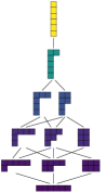
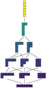
Figure 1: The values of power-sum kernels on $\operatorname{S}_{6}$, corresponding to $\boldsymbol{z}=(1/2,1/2)$, $(2/3,1/3)$, $(3/4,1/4)$ and $(4/5,1/5)$. The underlying graph is the quotient of the Cayley graph of $\operatorname{S}_{6}$ with vertices partitioned into conjugacy classes, given by Young diagrams.

2.2 Proof of the theorem 1

Yaglom’s theory [20] implies that bi-invariant kernels on compact groups can be described in terms of representation theory. In particular, any bi-invariant kernel $k:G\times G\to\mathbb{R}$ on a compact group $G$, whose identity element we denote by $e_{G}$, has the form

$$k(g,h)=k(gh^{-1},e_{G})=k(e_{G},g^{-1}h)=\sum_{\lambda}a_{\lambda}\chi_{\lambda}(gh^{-1}),$$ (10)

where $a_{\lambda}\geq 0$ and $\sum_{\lambda}a_{\lambda}d_{\lambda}<\infty$, the summation is over all irreducible unitary representations $\pi_{\lambda}$ of the group $G$, $\chi_{\lambda}\colon G\to\operatorname{\mathbb{C}}$ denotes the character of the representation $\pi_{\lambda}$, and $d_{\lambda}$ denotes its dimension. Moreover, any function of the form (10) is bi-invariant and positive semidefinite (thus a well-defined kernel).

The group $\operatorname{S}_{n}$ is finite, and therefore compact. The number of its irreducible unitary representations is finite. It is known that irreducible representations of the group $\operatorname{S}_{n}$ can be indexed by Young diagrams of size $n$. A Young diagram is the representation of a partition $\lambda$ in form of the table with rows of size $\lambda_{1},\lambda_{2},\ldots,\lambda_{\ell}$. In this case, the number $\ell$ is called the length of the Young diagram, and $n=\sum_{j=1}^{\ell}\lambda_{j}$ is called its weight. It known that the characters $\chi_{\lambda}$ in the case of $\operatorname{S}_{n}$ are real-valued and even integer [16, Section 13.1, Corollary 1].

Young diagrams are also closely related to the unitary group $\operatorname{U}(m)$: diagrams of length at most $m$ enumerate the irreducible representations of $\operatorname{U}(m)$. Moreover, there is a deep connection between the representations of $\operatorname{S}_{n}$ and $\operatorname{U}(m)$, expressed through the Schur–Weyl duality. The character $s_{\lambda}$ of the irreducible representation of the group $\operatorname{U}(m)$ corresponding to the Young diagram $\lambda$ can be expressed as the Schur polynomial in the eigenvalues $z_{1},\ldots,z_{m}$ of the unitary matrix $\mathbf{Z}$. Using Weyl’s formula [17, §7.15] it can be expressed by:

$$s_{\lambda}(\mathbf{Z})=s_{\lambda}(z_{1},\ldots,z_{m})=\frac{\det\left(z_{i}^{\lambda_{j}+m-j}\right)_{i,j=1}^{m}}{\det\left(z_{i}^{m-j}\right)_{i,j=1}^{m}},$$ (11)

where for $j$ greater than the length of $\lambda$ it is assumed that $\lambda_{j}=0$, and the denominator divides the numerator, implying that $s_{\lambda}$ is indeed a polynomial in the variables $z_{1},\ldots,z_{m}$. Note that representations of the group $\operatorname{U}(m)$ can be extended to representations of the ambient general linear group $\operatorname{GL}(m,\operatorname{\mathbb{C}})$, whose character is also given by Equation 11.

There is another representation for $s_{\lambda}$, given in terms of semistandard Young tableaux, which we will now define. Let $\lambda$ be a partition. A semistandard tableau of shape $\lambda$ is a Young diagram corresponding to the partition $\lambda$, filled with natural numbers in such a way that values do not decrease in rows and increase in columns. Polynomials $s_{\lambda}$ can be described as follows [17, §7.10]:

$$s_{\lambda}(\boldsymbol{z})=\sum_{T}\boldsymbol{z}^{T}=\sum_{T}\prod_{j=1}^{m}z_{j}^{t_{j}},$$ (12)

where the summation is over all semistandard tables $T$ of shape $\lambda$ filled with numbers from $1$ to $m$, and $t_{j}$ denotes the number of cells in the table $T$ containing the number $j$.

The set of polynomials $s_{\lambda}$, similarly to the set of polynomials $p_{\lambda}$, forms a basis of the space of symmetric polynomials, while the characters $\chi_{\lambda}$ of the group $\operatorname{S}_{n}$ define the elements of the basis change matrix. More formally, the following holds.

Theorem (Frobenius Formula, [10, §4.1]).

$$p_{\mu(g)}(z_{1},z_{2},\ldots,z_{m})=\sum\chi_{\lambda}(g)s_{\lambda}(z_{1},z_{2},\ldots,z_{m}),$$ (13)

where the sum is over all Young diagrams of weight $n$ and length at most $m$, that is, partitions $\lambda$ of $n$ into at most $m$ terms.

We are now ready to prove the theorem 1.

Using (13), we write

$$k_{\boldsymbol{z}}(g,h)=p_{\mu(gh^{-1})}(\boldsymbol{z})=\sum\chi_{\lambda}(gh^{-1})s_{\lambda}(z_{1},z_{2},\ldots,z_{m}).$$ (14)

Since $z_{j}\geq 0$ for $j=1,\ldots,n$ by assumption, we see from the equality (12) that $s_{\lambda}(z_{1},z_{2},\ldots,z_{n})\geq 0$. It follows that $k_{\boldsymbol{z}}$ is of form (10) and is therefore a bi-invariant covariance on $\operatorname{S}_{n}$.

Finally, by definition of $\mu(gh^{-1})$ we have $|\{\mu_{j}(gh^{-1})=r\}|=c_{r}$. Taking this into account and grouping polynomials by their respective values of $\mu_{j}$, we get

$$k_{\boldsymbol{z}}(g,h)=p_{\mu(gh^{-1})}(\boldsymbol{z})=p_{\mu_{j}(gh^{-1})}(\boldsymbol{z})=\prod_{r=1}^{n}p_{r}^{c_{r}}(\boldsymbol{z}).$$ (15)

3 Sampling power sum Gaussian processes

Here we discuss ways of sampling Gaussian processes with power sum covariance functions, i.e. computational algorithms for obtaining their (approximate) trajectories. Let $f$ be a centered Gaussian process on the group $\operatorname{S}_{n}$ with covariance $k\colon\operatorname{S}_{n}\times\operatorname{S}_{n}\to\mathbb{R}$. Let $\boldsymbol{f}=\left(f(g_{1}),\ldots,f(g_{n!})\right)^{\top}$, where $g_{1},\ldots,g_{n!}$ are arbitrarily enumerated elements of $\operatorname{S}_{n}$. Then $\boldsymbol{f}\sim\operatorname{N}(\boldsymbol{0},\mathbf{K})$, where $\mathbf{K}$ is the covariance matrix of the random vector $\boldsymbol{f}$. Its elements are $\mathbf{K}_{jr}=k(g_{j},g_{r})$. Sampling the process $f$ means sampling the vector $\boldsymbol{f}$. Let us write

$$\boldsymbol{f}=\mathbf{K}^{1/2}\boldsymbol{\varepsilon}, \boldsymbol{\varepsilon}\sim\operatorname{N}(\boldsymbol{0},\mathbf{I}),$$ (16)

where $\mathbf{K}^{1/2}$ is a root of the matrix $\mathbf{K}$ in the sense that $\left(\mathbf{K}^{1/2}\right)^{\top}\mathbf{K}^{1/2}=\mathbf{K}$, and $\mathbf{I}$ is the identity matrix of size $n!$.

The representation (16) makes it possible to algorithmically sample $f$ by 1) calculating the root $\mathbf{K}^{1/2}$, 2) sampling the standard normal vector $\boldsymbol{\varepsilon}\sim\operatorname{N}(\boldsymbol{0},\mathbf{I})$, and 3) computing the matrix-vector product $\mathbf{K}^{1/2}\boldsymbol{\varepsilon}$. Step (2) has computational complexity $O(n!)$, step (3) has computational complexity $O((n!)^{2})$, and step (1) has computational complexity $O((n!)^{3})$. This ultimately makes this approach untenable for computing. This is not surprising given its excessive generality and not even relying on bi-invariance in any way. In what follows, we propose other techniques that leverage bi-invariance to allow, albeit approximately, sampling $f$ in a much more computationally efficient way.

The first such technique is a special case of the generalized random phase Fourier features method proposed by [1] for modeling bi-invariant Gaussian processes on general compact groups.

Let $k\colon\operatorname{S}_{n}\times\operatorname{S}_{n}\to\mathbb{R}$ be a bi-invariant covariance. Then it is of form (10), i.e. $k(g,h)=\sum_{\lambda}a_{\lambda}\chi_{\lambda}(gh^{-1})$. Thus [1] gives

$$f(g)\approx\sum_{r=1}^{R}\frac{1}{\sqrt{L}}\sum_{l=1}^{L}w_{l}^{\lambda_{r}}\chi_{\lambda_{r}}(gu_{l}), w_{l}^{\lambda_{r}}\mathrel{{}\mathop{\sim}\limits^{\text{i.i.d.}}}\operatorname{N}\left(0,\frac{a_{\lambda_{r}}}{d_{\lambda_{r}}}\right),$$ (17)

where $u_{l}\mathrel{{}\mathop{\sim}\limits^{\text{i.i.d.}}}\operatorname{U}(\operatorname{S}_{n})$ with $\operatorname{U}(\operatorname{S}_{n})$ denoting the uniform distribution (Haar probability measure) on $\operatorname{S}_{n}$, $d_{\lambda}$ denotes the dimension of the representation $\pi_{\lambda}$, and $\lambda_{1},\ldots,\lambda_{R}$ correspond to the $R$ representations of the group $\operatorname{S}_{n}$ with the highest value $a_{\lambda}d_{\lambda}$. To apply this approach, one has to be able to find $R$ representations with the largest value $a_{\lambda}d_{\lambda}$. The number of representations of $\operatorname{S}_{n}$ grows as $\left(4n\sqrt{3}\right)^{-1}e^{\pi\sqrt{2n/3}}$ [8], thus it is not clear how to do this in a computationally tractable way. Because of this we propose another technique for approximate modeling that does not require such a search.

It is similar to the technique from [1] described above, but it is intended for bi-invariant processes on $\operatorname{S}_{n}$ specifically. To do this, we need some preliminaries.

As before, by $s_{\lambda}(\mathbf{X})$, where $\mathbf{X}\in\operatorname{GL}(m,\operatorname{\mathbb{C}})$ is a diagonalizable matrix, we denote $s_{\lambda}(x_{1},x_{2},\ldots,x_{m})$, where $x_{j}$ are eigenvalues of the matrix $\mathbf{X}$. By the symbol $\operatorname{N}_{\operatorname{\mathbb{C}}^{m\times m}}$ we denote the ensemble of random matrices of size $m\times m$ with complex entries of the form $\operatorname{N}(0,1/2)+i\operatorname{N}(0,1/2)$, where all real and imaginary parts are jointly independent. Then the following is true [15, 9]:

$$\operatorname*{\mathbb{E}}_{\mathbf{Z}\sim\operatorname{N}_{\operatorname{\mathbb{C}}^{m\times m}}}s_{\lambda}(\mathbf{A}\mathbf{Z})\overline{s_{\lambda}(\mathbf{A}\mathbf{Z})} =\pi^{-m^{2}}\int_{-\infty}^{\infty}s_{\lambda}(\mathbf{A}\mathbf{Z})\overline{s_{\lambda}(\mathbf{A}\mathbf{Z})}e^{-\operatorname{tr}(\mathbf{Z}\mathbf{Z}^{*})}\mathop{}\!\mathrm{d}\mathbf{Z}$$ (18)

$$=\frac{n!\cdot s_{\lambda}(\mathbf{A}\mathbf{A}^{*})}{d_{\lambda}}.$$

Also for any character $\chi_{\lambda}$ of an irreducible representation of $\operatorname{S}_{n}$ we have [1]

$$\frac{\chi_{\lambda}(gh^{-1})}{d_{\lambda}}=\int_{\operatorname{S}_{n}}\chi_{\lambda}(gu)\chi_{\lambda}(hu)=\operatorname*{\mathbb{E}}_{u\sim\operatorname{U}(\operatorname{S}_{n})}\chi_{\lambda}(gu)\chi_{\lambda}(hu).$$ (19)

Rewriting the right hand side of the formula (14) using (18) with

$$\mathbf{A}=\operatorname{diag}(\sqrt{z_{1}},\sqrt{z_{2}},\ldots,\sqrt{z_{m}})$$ (20)

and using Equation 19 afterwards, we get that

$$k_{\boldsymbol{z}}(gh^{-1}) =\sum_{\lambda}\chi_{\lambda}(gh^{-1})s_{\lambda}(z_{1},z_{2},\ldots,z_{m})$$ (21)

$$=\sum_{\lambda}\frac{d_{\lambda}^{2}}{n!}\operatorname*{\mathbb{E}}_{u\sim\operatorname{U}(\operatorname{S}_{n})}\operatorname*{\mathbb{E}}_{\mathbf{Z}\sim\operatorname{N}_{\operatorname{\mathbb{C}}^{m\times m}}}\chi_{\lambda}(gu)\chi_{\lambda}(hu)s_{\lambda}(\mathbf{A}\mathbf{Z})\overline{s_{\lambda}(\mathbf{A}\mathbf{Z})}.$$

Finally, we need some properties of the Robinson—Schensted algorithm [14]. Given a permutation $g\in\operatorname{S}_{n}$, this algorithm constructs in a bijective way a pair of standard Young tableaux $(P(g),Q(g))$ of the same shape $\lambda(g)$. We omit all the detail details concerning this mapping, but note only that there is an implementation with computational complexity $O(n^{3/2})$ [19]. For $\lambda(g)$ from the Robinson—Schensted algorithm and for $g\sim\operatorname{U}(\operatorname{S}_{n})$ the equality $\operatorname{\mathbb{P}}(\lambda(g)=\lambda)=d_{\lambda}^{2}/n!$ holds. Therefore, summing over $\lambda$ in the expression (LABEL:eqn:sampling_before_rh) can be rewritten so that

$$k_{x}(gh^{-1})=\operatorname*{\mathbb{E}}_{\begin{subarray}{c}v,u\sim\operatorname{U}(\operatorname{S}_{n})\\ \mathbf{Z}\sim\operatorname{N}_{\operatorname{\mathbb{C}}^{m\times m}}\end{subarray}}\chi_{\lambda(v)}(gu)\chi_{\lambda(v)}(hu)s_{\lambda(v)}(\mathbf{A}\mathbf{Z})\overline{s_{\lambda(v)}(\mathbf{A}\mathbf{Z})}.$$ (22)

As a result, we obtain the desired approximation of the following form:

$$f(g)\approx\frac{1}{\sqrt{L}}\sum_{j=1}^{L}\left(w_{j,1}\operatorname{Re}s_{\lambda(v_{j})}(\mathbf{A}\mathbf{Z}_{j})+w_{j,2}\operatorname{Im}s_{\lambda(v_{j})}(\mathbf{A}\mathbf{Z}_{j})\right)\chi_{\lambda(v_{j})}(gu_{j}),$$ (23)

with random coefficients $w_{j,1}\mathrel{{}\mathop{\sim}\limits^{\text{i.i.d.}}}\operatorname{N}(0,1)$, $w_{j,2}\mathrel{{}\mathop{\sim}\limits^{\text{i.i.d.}}}\operatorname{N}(0,1)$, and indices $v_{j}\mathrel{{}\mathop{\sim}\limits^{\text{i.i.d.}}}U(\operatorname{S}_{n})$, $u_{j}\mathrel{{}\mathop{\sim}\limits^{\text{i.i.d.}}}U(\operatorname{S}_{n})$, $\mathbf{Z}_{j}\mathrel{{}\mathop{\sim}\limits^{\text{i.i.d.}}}\operatorname{N}_{\operatorname{\mathbb{C}}^{m\times m}}$.

References

- [1] Iskander Azangulov, Andrei Smolensky, Alexander Terenin and Viacheslav Borovitskiy “Stationary Kernels and Gaussian Processes on Lie Groups and their Homogeneous Spaces I: the Compact Case” In arXiv preprint arXiv:2208.14960, 2022
- [2] François Bachoc, Baptiste Broto, Fabrice Gamboa and Jean-Michel Loubes “Gaussian field on the symmetric group: Prediction and learning” In Electronic Journal of Statistics 14.1 Institute of Mathematical StatisticsBernoulli Society, 2020, pp. 503–546
- [3] Serge Cohen and Jacques Istas “Fractional Fields and Applications” 73, Mathématiques et Applications Springer, 2013
- [4] Serge Cohen and MA Lifshits “Stationary Gaussian random fields on hyperbolic spaces and on Euclidean spheres” In ESAIM: Probability and Statistics 16 EDP Sciences, 2012, pp. 165–221
- [5] D. Corfield, H. Sati and U. Schreiber “Fundamental weight systems are quantum states” In arXiv preprint arXiv:2105.02871, 2021
- [6] Sam Coveney et al. “Gaussian process manifold interpolation for probabilistic atrial activation maps and uncertain conduction velocity” In Philosophical Transactions of the Royal Society A 378.2173, 2020, pp. 20190345
- [7] Persi Diaconis “Group Representations in Probability and Statistics” 11, IMS Lecture Notes Monogr. Ser., 1988
- [8] Paul Erdős “On an Elementary Proof of Some Asymptotic Formulas in the Theory of Partitions” In Annals of Mathematics 43.3 Annals of Mathematics, 1942, pp. 437–450
- [9] Peter J Forrester and Eric M Rains “Matrix averages relating to Ginibre ensembles” In Journal of Physics A: Mathematical and Theoretical 42.38 IOP Publishing, 2009, pp. 385205
- [10] William Fulton and Joe Harris “Representation theory: a first course” 129, Graduate Texts in Mathematics Springer-Verlag, 1991
- [11] Michael Hutchinson et al. “Vector-valued Gaussian Processes on Riemannian Manifolds via Gauge Independent Projected Kernels” In Advances in Neural Information Processing Systems 34, 2021, pp. 17160–17169
- [12] Jacques Istas “Spherical and Hyperbolic Fractional Brownian Motion” In Electronic Communications in Probability 10 Institute of Mathematical StatisticsBernoulli Society, 2005, pp. 254–262
- [13] Noémie Jaquier et al. “Geometry-aware Bayesian Optimization in Robotics using Riemannian Matérn Kernels” In Conference on Robot Learning, 2022, pp. 794–805 PMLR
- [14] D.E. Knuth “The Art of Computer Programming: Volume 3: Sorting and Searching” Pearson Education, 1998
- [15] A.. Orlov “Tau Functions and Matrix Integrals” arXiv, 2002
- [16] J.-P. Serre “Linear Representations of Finite Groups” Springer, 1977
- [17] R.P. Stanley and S. Fomin “Enumerative Combinatorics: Volume 2”, Cambridge Studies in Advanced Mathematics Cambridge University Press, 1997
- [18] Jonathan E Taylor and Robert J Adler “Euler characteristics for Gaussian fields on manifolds” In The Annals of Probability 31.2 Institute of Mathematical Statistics, 2003, pp. 533–563
- [19] Alexander Tiskin “Fast RSK Correspondence by Doubling Search” In 30th Annual European Symposium on Algorithms (ESA 2022) 244, Leibniz International Proceedings in Informatics (LIPIcs) Schloss Dagstuhl – Leibniz-Zentrum für Informatik, 2022, pp. 86:1–86:10
- [20] A.. Yaglom “Second-order homogeneous random fields” In Proceedings of the Fourth Berkeley Symposium on Mathematical Statistics and Probability, Volume 2: Contributions to Probability Theory, 1961, pp. 593–622 University of California Press