Smearing lattice gauge fields on a quantum computer
Abstract
Smearing of gauge-field configurations in lattice field theory improves the results of lattice simulations by suppressing high energy modes from correlation functions. In quantum simulations, high kinetic energy eigenstates are introduced when the time evolution operator is approximated such as Trotterization. While improved Trotter product formulae exist to reduce the errors, they have diminishing accuracy returns with respect to resource costs. Therefore having an algorithm that has fewer resources than an improved Trotter formula is desirable. In this work I develop a representation agnostic method for quantum smearing and show that it reduces the coupling to high energy modes in the discrete nonabelian gauge theory .
1 Introduction. Classical lattice gauge theory (LGT) offers the ability for high precision determinations of observables such as decay constants, hadron masses, scattering amplitudes below multiparticle thresholds, finite temperature QCD, and equations of state [1, 2, 3, 4, 5, 6, 7, 8, 9]. However, these simulations struggle to extract multiparticle threshold final states and dynamical quantities such as viscosities which encounter sign problems using stochastic methods [10, 11]. Quantum computers offer a method to circumvent this sign problem entirely by using a Hamiltonian formulation for the deterministic evolution of a quantum system [12, 13, 14].
There has been a significant effort to develop methods for simulating LGTs on quantum computers [15, 16, 17, 18, 19, 20, 21, 22, 23, 24, 25, 26, 27, 28, 29, 30, 31, 32, 33, 34, 35, 36, 37, 38, 39, 40, 41, 42, 43, 44, 45, 46, 47, 48, 49, 50, 51, 52, 53, 54, 55, 56, 57, 58, 59, 60, 61, 62, 63, 64, 65, 66, 67, 68, 69, 70, 71, 72, 73]. The benefits for high energy physics from quantum simulators stems from the ability to do real-time simulations and study finite density physics. However it is known that many time evolution methods introduce couplings to other energy modes which is undesirable [74, 75, 40].
Implementations of the time evolution operator for quantum simulations involve approximating this operator [76, 77, 78, 79, 80, 81, 82, 83, 84, 85, 86]. One method, Trotterization, break the Hamiltonian, , is broken into commuting terms, e.g. potential () and kinetic (), such that , which are easily implemented on a quantum computer [76, 77, 87]. All approximations distort the Hamiltonian spectrum. Trotterization affects the spectrum by introducing terms proportional to multiplied by commutators such as ; this significantly affects observables such as time dependent correlation functions [74]. The spectrum distortion induces couplings to other energy states [88, 75]. Therefore one wants a band-pass filter that cuts out the energy modes unconnected to the states of interest; higher order Trotter product formulae do this [77]. However, higher order Trotter products become increasingly more expensive in terms of gates and have diminishing accuracy returns [89]. The gate costs for quantum electrodynamics (QED) and quantum chromodynamics (QCD) simulations in Ref. [90] is expensive; therefore, finding methods to bring these costs down is crucial. One method would be finding an alternative way to bring down the systematic errors from approximate time evolution (APE) other than improved operators.
Classical LGT theory developed tools such as smearing [91, 92, 93, 94, 95, 96, 97, 98, 99, 100] and gradient flow [101, 102, 103, 104] as a method for dealing with high energy states in lattice configurations. This allows for classical simulations with fewer statistics and coarser lattices [105, 106, 100, 107]. All smearing methods averages neighboring fluctuations on a lattice configuration to remove ultraviolet (UV) contamination; gradient flow moves the configuration along the renormalization group and dampens high-momentum field modes which can be used as a continuous method of smearing [102, 108, 103, 109]. In addition smearing comes in two forms: operator smearing and link smearing. Operator smearing mitigates the excited state contamination from a lattice operator choices, link smearing suppresses the noise from UV fluctuations from the background field configurations themselves. Since one does not know the UV state explicitly one approximates them by the using the kinetic energy operator as a proxy.
Therefore one would like to have a quantum equivalent of classical lattice link smearing that is both cost effective and removes some couplings to high energy modes induced by approximate time evolution or state preparation. The quantum case of smearing can be understood as introducing a small imaginary component to the kinetic energy operator that will suppress their contribution to time dependent observables. In many cases these non-unitary algorithms can yield shorter local circuits than their unitary counter parts at the expense of some probability of failure [110, 111, 112, 40, 113, 114].
In this context one can estimate the cost of smearing for a larger group that could approximate QCD, . Using the chosen smearing strength is from Ref [115] as an approximate value for the smearing parameter used for a quantum simulation of , the quantum smearing operator has an approximate nonunitarity of for a single link using the definition of in Ref. [116]. If one estimates that a stochastic implementation such as in [113] of the non-unitary operator succeeds with probability , then every time all the links are smeared it will succeed with probability where is the number of dimensions and is the number of sites on the lattice in one direction. Using the volume as an estimate for gluon viscosity from Ref. [90], this would imply that for a lattice using smearing 50 times would succeed stochastically with probability . This is nearly impossible and the unitary method provided in this work would win out even with a subexponential increase in the number of required qubits.
In this letter, I develop a unitary quantum smearing algorithm based on classical stout smearing in a representation agnostic way. This quantum smearing algorithm scales linearly with the number of qubits and circuit depth compared to exponential costs with nonunitary operators. Using a discrete nonabelian gauge theory on a lattice I demonstrate that the high energy modes are suppressed and the underlying physics is not distorted.
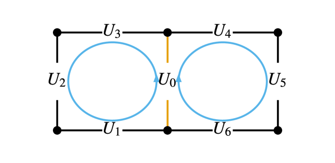
2 Stout smearing as a classical algorithm. Stout smearing takes a linear combination of plaquettes connected to a link, see Fig. 1, and then uses an exponential mapping of the linear combinations to transform the target link to a smeared link. The benefits of this smearing algorithm are that it smears out fluctuations at the lattice scale, preserves group structure, and is gauge invariant. Following the notation in Ref. [97], I cover the basics of stout smearing.
The staples connected to our target link in the direction are defined as
| (1) |
this is the sum of the plaquettes in Fig. 1. Next, one defines the linear combination of plaquettes as
| (2) |
A new variable, , defined as
| (3) |
creates a traceless Hermitian matrix which is a generator for a group element. The target link is then transformed to
| (4) |
where is a tunable parameter to determine how strong the smearing is and indicates that some projection back onto the group may be required if the group is not sufficiently continuous. Hereinafter the element will be referred to as the shift element, . A graphical depiction of these terms is shown in Fig. 1.
3 Stout smearing as a quantum algorithm. A direct mapping of smearing encounters difficulties because it requires making a copy of the lattice; this is not allowed in quantum computation [117, 118, 119, 120, 121]. The copying procedure is required to avoid stroboscopic approximations. Therefore we need to alter the smearing algorithm to allow for reversibility which increases the required physical quantum resources compared to the classical algorithm.
Before introducing the algorithm, I will cover the necessary quantum operations needed for this algorithm. One requires three primitive group operations: which multiplies two group elements together, which inverts a group element, and which generates the shift elements. The algorithm is summarized in Fig. 2.

This algorithm is representation agnostic; any Hamiltonian formulation requires a method to represent group element basis states. However, the process of implementing , , and is representation dependent. Nevertheless, given group element basis exists this the function is equivalent to a function that takes as inputs numbers and outputs a new number onto a clean scratch register which is a valid unitary operation on a quantum computer [117]. A side effect of this algorithm is that a new lattice’s worth of qubits is required every time the smearing operation is applied in order to ensure reversibility. Therefore there is a linear cost in the number of qubits to use this algorithm.
We show in Fig. 3 how to construct the state on an ancilla register for any group and formulation. It is straight forward once all shift elements have been constructed to multiply these elements with their corresponding physical lattice link using the operator.
4 gauge theory example. It is illustrative to demonstrate smearing by a using discrete group which has the benefit of being defined explicitly in the group element basis. A dihedral group, , whose primitive gates have been derived in Refs. [122, 123], is useful as a proof of principle example. The elements of the group are with and and are two of the Pauli matrices. A group element is repesented by the qubit state . This example uses a two plaquette theory with periodic boundary conditions as shown in Fig. 5 The Hamiltonian for this theory is
| (5) |
where is the kinetic term of the Hamiltonian, , and is defined in [122] and is the potential term of the Hamiltonian, . In this example .
An implementation of for is necessary. The realization of the circuit depends on the chosen value of . In order to ensure that smearing occurs but is not too significant that it distorts the underlying physics, let . For less than this value no smearing will take place. Since is discrete, within given ranges will yield the same . Fig. 5 shows the implementation of this quantum circuit for . The time evolution operator , where is the Trotterization order, is at second order
| (6) |
and third order
| (7) |
where and are the kinetic and potential parts of the Hamiltonian. For these simulations . This is an example which shows contributions from other eigenstates.


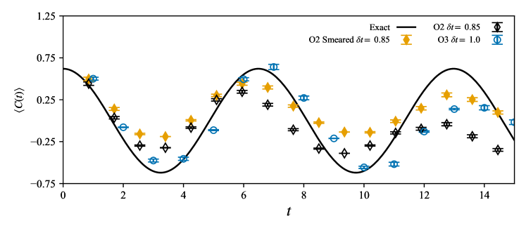
Fig. 6 shows the time evolution with , of the plaquette correlator,
| (8) |
where is the gauge invariant ground state, is the gauge invariant projection of the first excited state, and is the plaquette . A third order Trotterization at which has nearly the same root mean square error as the smeared evolution is also shown. While the third order Trotterization is superior to the second order Trotterization with and with out smearing before , afterwards the higher energy states begin to distort the time evolution which is expected for a coarse Trotterization and aligns with the second order smeared Trotterization. The ancilla registers are reset in order to minimize the memory resource requirements on the classical simulations.
It is worth examining the resource costs of smearing in a fault tolerant perspective. Many error correcting codes for fault tolerant quantum computing have costly single qubit rotation operations such as the T-gate [124, 125, 126, 127, 128, 129]. For this reason T-gates are an important metric for algorithm costs on fault tolerant quantum computers.
| operator | T gates |
|---|---|
| 2nd order Trotter | 696 + 46 |
| 3rd order Trotter | 1008 + 131.1 |
| smearing | 560 |
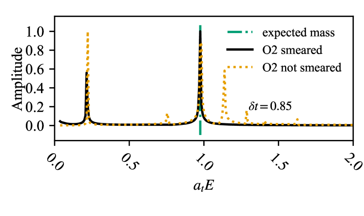
The T-gate costs of a single second order Trotter step for , third order Trotter, and the smearing operator on the whole lattice in Tab. 1. These costs are derived from the gates provided in Refs. [122, 123] and the single qubit gates are approximated using the repeat until success method with T gate cost where is the desired gate infidelity [130]. The total cost for third order Trotterization for infidelity, and requires 1.75 times more T gates than a second order Trotterization at with smearing and 2.5 times as many T-gates if the third order Trotterization is used with . This T gate saving should increase for larger groups as the projection operation will not require approximations using T-gate synthesis. The second order smeared evolution has fewer high energy oscillations than the unsmeared evolution. Information regarding energy states can be extracted from the fourier spectrum of the time series data. Examining the Fourier spectrum for the smeared and unsmeared evolution using second order Trotterization (see Fig. 7) shows that many high kinetic energy modes are mitigated. It is found that smearing does not uniformly suppress higher order energies.
5. Conclusions This work developed a unitary algorithm for smearing real-time quantum simulations of LGTS. Somewhat analogously to classical LGT, this algorithm acts as expected by reducing higher energy modes. For the small lattice size investigated the benefits of smearing are noticable and achieves a factor of 2 reduction in T-gates compared to improved Trotterization. The computational costs scale linearly with the number of times smearing is applied compared to exponential costs for nonunitary evolution. The representation agnostic method in which this algorithm is presented allows it to be applied to a wide range of Hamiltonian formulations [131, 43, 132, 133, 134, 135, 136, 50, 71, 137, 138, 139, 140, 141, 142, 143, 144, 115, 123, 145, 146, 147, 148, 149]for quantum simulation of LGTs and will likely bring down the cost of many fault tolerant applications. This opens the way to build smearing algorithms for larger groups that could approximate and as well as extend the method to the inclusion of dynamical fermions.
Acknowledgements.
I wish to thank Mike Wagman, Ruth Van de Water, Norman Tubman, Stuart Hadfield, Henry Lamm, Judah Unmuth-Yockey, and Matthew Reagor for comments and advice. This work is supported by the DOE QuantISED program through the theory consortium “Intersections of QIS and Theoretical Particle Physics” at Fermilab and by the U.S. Department of Energy. Fermilab is operated by Fermi Research Alliance, LLC under contract number DE-AC02-07CH11359 with the United States Department of Energy.References
- Detmold et al. [2019] W. Detmold, R. G. Edwards, J. J. Dudek, M. Engelhardt, H.-W. Lin, S. Meinel, K. Orginos, and P. Shanahan (USQCD), Hadrons and Nuclei, Eur. Phys. J. A 55, 193 (2019), arXiv:1904.09512 [hep-lat] .
- Aoyama et al. [2020] T. Aoyama et al., The anomalous magnetic moment of the muon in the Standard Model, Phys. Rept. 887, 1 (2020), arXiv:2006.04822 [hep-ph] .
- Aoki et al. [2022] Y. Aoki et al. (Flavour Lattice Averaging Group (FLAG)), FLAG Review 2021, Eur. Phys. J. C 82, 869 (2022), arXiv:2111.09849 [hep-lat] .
- Kronfeld et al. [2022] A. S. Kronfeld et al. (USQCD), Lattice QCD and Particle Physics (2022), arXiv:2207.07641 [hep-lat] .
- Bazavov et al. [2019a] A. Bazavov, F. Karsch, S. Mukherjee, and P. Petreczky (USQCD), Hot-dense Lattice QCD: USQCD whitepaper 2018, Eur. Phys. J. A 55, 194 (2019a), arXiv:1904.09951 [hep-lat] .
- Boyle et al. [2022] P. A. Boyle et al., A lattice QCD perspective on weak decays of and quarks Snowmass 2022 White Paper, in 2022 Snowmass Summer Study (2022) arXiv:2205.15373 [hep-lat] .
- Kronfeld et al. [2019] A. S. Kronfeld, D. G. Richards, W. Detmold, R. Gupta, H.-W. Lin, K.-F. Liu, A. S. Meyer, R. Sufian, and S. Syritsyn (USQCD), Lattice QCD and Neutrino-Nucleus Scattering, Eur. Phys. J. A 55, 196 (2019), arXiv:1904.09931 [hep-lat] .
- Davoudi et al. [2022] Z. Davoudi et al., Report of the Snowmass 2021 Topical Group on Lattice Gauge Theory, in 2022 Snowmass Summer Study (2022) arXiv:2209.10758 [hep-lat] .
- Briceño et al. [2018] R. A. Briceño, J. J. Dudek, and R. D. Young, Scattering processes and resonances from lattice QCD, Reviews of Modern Physics 90, 10.1103/revmodphys.90.025001 (2018).
- de Forcrand [2009] P. de Forcrand, Simulating QCD at finite density, PoS LAT2009, 010 (2009), arXiv:1005.0539 [hep-lat] .
- Tripolt et al. [2019] R.-A. Tripolt, P. Gubler, M. Ulybyshev, and L. Von Smekal, Numerical analytic continuation of Euclidean data, Comput. Phys. Commun. 237, 129 (2019), arXiv:1801.10348 [hep-ph] .
- Feynman [1982] R. P. Feynman, Simulating physics with computers, Int. J. Theor. Phys. 21, 467 (1982).
- Jordan et al. [2014] S. P. Jordan, K. S. M. Lee, and J. Preskill, Quantum Computation of Scattering in Scalar Quantum Field Theories, Quant. Inf. Comput. 14, 1014 (2014), arXiv:1112.4833 [hep-th] .
- Jordan et al. [2012] S. P. Jordan, K. S. M. Lee, and J. Preskill, Quantum Algorithms for Quantum Field Theories, Science 336, 1130 (2012), arXiv:1111.3633 [quant-ph] .
- Banerjee et al. [2012] D. Banerjee, M. Dalmonte, M. Muller, E. Rico, P. Stebler, U. J. Wiese, and P. Zoller, Atomic Quantum Simulation of Dynamical Gauge Fields coupled to Fermionic Matter: From String Breaking to Evolution after a Quench, Phys. Rev. Lett. 109, 175302 (2012), arXiv:1205.6366 [cond-mat.quant-gas] .
- Mueller et al. [2022] N. Mueller, J. A. Carolan, A. Connelly, Z. Davoudi, E. F. Dumitrescu, and K. Yeter-Aydeniz, Quantum computation of dynamical quantum phase transitions and entanglement tomography in a lattice gauge theory (2022), arXiv:2210.03089 [quant-ph] .
- Ciavarella et al. [2022] A. Ciavarella, N. Klco, and M. J. Savage, Some Conceptual Aspects of Operator Design for Quantum Simulations of Non-Abelian Lattice Gauge Theories (2022) arXiv:2203.11988 [quant-ph] .
- Zohar et al. [2012] E. Zohar, J. I. Cirac, and B. Reznik, Simulating Compact Quantum Electrodynamics with ultracold atoms: Probing confinement and nonperturbative effects, Phys. Rev. Lett. 109, 125302 (2012), arXiv:1204.6574 [quant-ph] .
- Zohar et al. [2013a] E. Zohar, J. I. Cirac, and B. Reznik, Cold-Atom Quantum Simulator for SU(2) Yang-Mills Lattice Gauge Theory, Phys. Rev. Lett. 110, 125304 (2013a), arXiv:1211.2241 [quant-ph] .
- Zohar et al. [2013b] E. Zohar, J. I. Cirac, and B. Reznik, Quantum simulations of gauge theories with ultracold atoms: local gauge invariance from angular momentum conservation, Phys. Rev. A88, 023617 (2013b), arXiv:1303.5040 [quant-ph] .
- Zohar and Burrello [2015] E. Zohar and M. Burrello, Formulation of lattice gauge theories for quantum simulations, Phys. Rev. D91, 054506 (2015), arXiv:1409.3085 [quant-ph] .
- Zohar et al. [2016] E. Zohar, J. I. Cirac, and B. Reznik, Quantum Simulations of Lattice Gauge Theories using Ultracold Atoms in Optical Lattices, Rept. Prog. Phys. 79, 014401 (2016), arXiv:1503.02312 [quant-ph] .
- Zohar et al. [2017] E. Zohar, A. Farace, B. Reznik, and J. I. Cirac, Digital lattice gauge theories, Phys. Rev. A95, 023604 (2017), arXiv:1607.08121 [quant-ph] .
- Klco et al. [2020] N. Klco, J. R. Stryker, and M. J. Savage, SU(2) non-Abelian gauge field theory in one dimension on digital quantum computers, Phys. Rev. D 101, 074512 (2020), arXiv:1908.06935 [quant-ph] .
- Ciavarella et al. [2021a] A. Ciavarella, N. Klco, and M. J. Savage, A Trailhead for Quantum Simulation of SU(3) Yang-Mills Lattice Gauge Theory in the Local Multiplet Basis (2021a), arXiv:2101.10227 [quant-ph] .
- Bender et al. [2018] J. Bender, E. Zohar, A. Farace, and J. I. Cirac, Digital quantum simulation of lattice gauge theories in three spatial dimensions, New J. Phys. 20, 093001 (2018), arXiv:1804.02082 [quant-ph] .
- Liu and Xin [2020] J. Liu and Y. Xin, Quantum simulation of quantum field theories as quantum chemistry (2020), arXiv:2004.13234 [hep-th] .
- Hackett et al. [2019] D. C. Hackett, K. Howe, C. Hughes, W. Jay, E. T. Neil, and J. N. Simone, Digitizing Gauge Fields: Lattice Monte Carlo Results for Future Quantum Computers, Phys. Rev. A 99, 062341 (2019), arXiv:1811.03629 [quant-ph] .
- Alexandru et al. [2019a] A. Alexandru, P. F. Bedaque, S. Harmalkar, H. Lamm, S. Lawrence, and N. C. Warrington (NuQS), Gluon field digitization for quantum computers, Phys.Rev.D 100, 114501 (2019a), arXiv:1906.11213 [hep-lat] .
- Yamamoto [2021] A. Yamamoto, Real-time simulation of (2+1)-dimensional lattice gauge theory on qubits, PTEP 2021, 013B06 (2021), arXiv:2008.11395 [hep-lat] .
- Haase et al. [2021] J. F. Haase, L. Dellantonio, A. Celi, D. Paulson, A. Kan, K. Jansen, and C. A. Muschik, A resource efficient approach for quantum and classical simulations of gauge theories in particle physics, Quantum 5, 393 (2021), arXiv:2006.14160 [quant-ph] .
- Armon et al. [2021] T. Armon, S. Ashkenazi, G. García-Moreno, A. González-Tudela, and E. Zohar, Photon-mediated Stroboscopic Quantum Simulation of a Lattice Gauge Theory (2021), arXiv:2107.13024 [quant-ph] .
- Bazavov et al. [2019b] A. Bazavov, S. Catterall, R. G. Jha, and J. Unmuth-Yockey, Tensor renormalization group study of the non-abelian higgs model in two dimensions, Phys. Rev. D 99, 114507 (2019b).
- Honda et al. [2022] M. Honda, E. Itou, Y. Kikuchi, and Y. Tanizaki, Negative string tension of a higher-charge Schwinger model via digital quantum simulation, PTEP 2022, 033B01 (2022), arXiv:2110.14105 [hep-th] .
- Bazavov et al. [2015a] A. Bazavov, Y. Meurice, S.-W. Tsai, J. Unmuth-Yockey, and J. Zhang, Gauge-invariant implementation of the Abelian Higgs model on optical lattices, Phys. Rev. D92, 076003 (2015a), arXiv:1503.08354 [hep-lat] .
- Zhang et al. [2018a] J. Zhang, J. Unmuth-Yockey, J. Zeiher, A. Bazavov, S. W. Tsai, and Y. Meurice, Quantum simulation of the universal features of the Polyakov loop, Phys. Rev. Lett. 121, 223201 (2018a), arXiv:1803.11166 [hep-lat] .
- Unmuth-Yockey et al. [2018a] J. Unmuth-Yockey, J. Zhang, A. Bazavov, Y. Meurice, and S.-W. Tsai, Universal features of the Abelian Polyakov loop in 1+1 dimensions, Phys. Rev. D98, 094511 (2018a), arXiv:1807.09186 [hep-lat] .
- Unmuth-Yockey [2019] J. F. Unmuth-Yockey, Gauge-invariant rotor Hamiltonian from dual variables of 3D gauge theory, Phys. Rev. D 99, 074502 (2019), arXiv:1811.05884 [hep-lat] .
- Kreshchuk et al. [2020a] M. Kreshchuk, W. M. Kirby, G. Goldstein, H. Beauchemin, and P. J. Love, Quantum Simulation of Quantum Field Theory in the Light-Front Formulation (2020a), arXiv:2002.04016 [quant-ph] .
- Gustafson [2020] E. Gustafson, Projective Cooling for the transverse Ising model, Phys. Rev. D 101, 071504 (2020), arXiv:2002.06222 [hep-lat] .
- Gustafson et al. [2021] E. Gustafson, B. Holzman, J. Kowalkowski, H. Lamm, A. C. Y. Li, G. Perdue, S. Boixo, S. Isakov, O. Martin, R. Thomson, C. Vollgraff Heidweiller, J. Beall, M. Ganahl, G. Vidal, and E. Peters, Large scale multi-node simulations of gauge theory quantum circuits using Google Cloud Platform, arXiv e-prints , arXiv:2110.07482 (2021), arXiv:2110.07482 [quant-ph] .
- Kreshchuk et al. [2020b] M. Kreshchuk, S. Jia, W. M. Kirby, G. Goldstein, J. P. Vary, and P. J. Love, Simulating Hadronic Physics on NISQ devices using Basis Light-Front Quantization (2020b), arXiv:2011.13443 [quant-ph] .
- Raychowdhury and Stryker [2018] I. Raychowdhury and J. R. Stryker, Solving Gauss’s Law on Digital Quantum Computers with Loop-String-Hadron Digitization (2018), arXiv:1812.07554 [hep-lat] .
- Raychowdhury and Stryker [2020a] I. Raychowdhury and J. R. Stryker, Loop, String, and Hadron Dynamics in SU(2) Hamiltonian Lattice Gauge Theories, Phys. Rev. D 101, 114502 (2020a), arXiv:1912.06133 [hep-lat] .
- Chakraborty et al. [2022] B. Chakraborty, M. Honda, T. Izubuchi, Y. Kikuchi, and A. Tomiya, Classically emulated digital quantum simulation of the Schwinger model with a topological term via adiabatic state preparation, Phys. Rev. D 105, 094503 (2022), arXiv:2001.00485 [hep-lat] .
- Wang et al. [2022] H.-Y. Wang, W.-Y. Zhang, Z.-Y. Yao, Y. Liu, Z.-H. Zhu, Y.-G. Zheng, X.-K. Wang, H. Zhai, Z.-S. Yuan, and J.-W. Pan, Interrelated Thermalization and Quantum Criticality in a Lattice Gauge Simulator (2022), arXiv:2210.17032 [cond-mat.quant-gas] .
- Davoudi et al. [2021] Z. Davoudi, I. Raychowdhury, and A. Shaw, Search for efficient formulations for Hamiltonian simulation of non-Abelian lattice gauge theories, Phys. Rev. D 104, 074505 (2021), arXiv:2009.11802 [hep-lat] .
- Wiese [2014] U.-J. Wiese, Towards Quantum Simulating QCD, Proceedings, 24th International Conference on Ultra-Relativistic Nucleus-Nucleus Collisions (Quark Matter 2014): Darmstadt, Germany, May 19-24, 2014, Nucl. Phys. A931, 246 (2014), arXiv:1409.7414 [hep-th] .
- Luo et al. [2019] D. Luo, J. Shen, M. Highman, B. K. Clark, B. DeMarco, A. X. El-Khadra, and B. Gadway, A Framework for Simulating Gauge Theories with Dipolar Spin Systems (2019), arXiv:1912.11488 [quant-ph] .
- Brower et al. [2020] R. C. Brower, D. Berenstein, and H. Kawai, Lattice Gauge Theory for a Quantum Computer, PoS LATTICE2019, 112 (2020), arXiv:2002.10028 [hep-lat] .
- Mathis et al. [2020] S. V. Mathis, G. Mazzola, and I. Tavernelli, Toward scalable simulations of Lattice Gauge Theories on quantum computers, Phys. Rev. D 102, 094501 (2020), arXiv:2005.10271 [quant-ph] .
- Singh [2019] H. Singh, Qubit nonlinear sigma models (2019), arXiv:1911.12353 [hep-lat] .
- Singh and Chandrasekharan [2019] H. Singh and S. Chandrasekharan, Qubit regularization of the sigma model, Phys. Rev. D 100, 054505 (2019), arXiv:1905.13204 [hep-lat] .
- Buser et al. [2020] A. J. Buser, T. Bhattacharya, L. Cincio, and R. Gupta, Quantum simulation of the qubit-regularized O(3)-sigma model (2020), arXiv:2006.15746 [quant-ph] .
- Bhattacharya et al. [2020] T. Bhattacharya, A. J. Buser, S. Chandrasekharan, R. Gupta, and H. Singh, Qubit regularization of asymptotic freedom (2020), arXiv:2012.02153 [hep-lat] .
- Barata et al. [2020] J. a. Barata, N. Mueller, A. Tarasov, and R. Venugopalan, Single-particle digitization strategy for quantum computation of a scalar field theory (2020), arXiv:2012.00020 [hep-th] .
- Kreshchuk et al. [2020c] M. Kreshchuk, S. Jia, W. M. Kirby, G. Goldstein, J. P. Vary, and P. J. Love, Light-Front Field Theory on Current Quantum Computers (2020c), arXiv:2009.07885 [quant-ph] .
- Ji et al. [2020a] Y. Ji, H. Lamm, and S. Zhu (NuQS), Gluon Field Digitization via Group Space Decimation for Quantum Computers, Phys. Rev. D 102, 114513 (2020a), arXiv:2005.14221 [hep-lat] .
- Bauer and Grabowska [2021] C. W. Bauer and D. M. Grabowska, Efficient Representation for Simulating U(1) Gauge Theories on Digital Quantum Computers at All Values of the Coupling (2021), arXiv:2111.08015 [hep-ph] .
- Gustafson [2021] E. Gustafson, Prospects for Simulating a Qudit Based Model of (1+1)d Scalar QED, Phys. Rev. D 103, 114505 (2021), arXiv:2104.10136 [quant-ph] .
- Hartung et al. [2022] T. Hartung, T. Jakobs, K. Jansen, J. Ostmeyer, and C. Urbach, Digitising SU(2) gauge fields and the freezing transition, Eur. Phys. J. C 82, 237 (2022), arXiv:2201.09625 [hep-lat] .
- Grabowska et al. [2022] D. M. Grabowska, C. Kane, B. Nachman, and C. W. Bauer, Overcoming exponential scaling with system size in Trotter-Suzuki implementations of constrained Hamiltonians: 2+1 U(1) lattice gauge theories (2022), arXiv:2208.03333 [quant-ph] .
- Murairi et al. [2022] E. M. Murairi, M. J. Cervia, H. Kumar, P. F. Bedaque, and A. Alexandru, How many quantum gates do gauge theories require? (2022), arXiv:2208.11789 [hep-lat] .
- Jahin et al. [2022] A. Jahin, A. C. Y. Li, T. Iadecola, P. P. Orth, G. N. Perdue, A. Macridin, M. Sohaib Alam, and N. M. Tubman, Fermionic approach to variational quantum simulation of Kitaev spin models, Phys. Rev. A 106, 022434 (2022), arXiv:2204.05322 [quant-ph] .
- Farrell et al. [2022a] R. C. Farrell, I. A. Chernyshev, S. J. M. Powell, N. A. Zemlevskiy, M. Illa, and M. J. Savage, Preparations for Quantum Simulations of Quantum Chromodynamics in 1+1 Dimensions: (II) Single-Baryon -Decay in Real Time (2022a), arXiv:2209.10781 [quant-ph] .
- Li et al. [2022] A. C. Y. Li, A. Macridin, S. Mrenna, and P. Spentzouris, Simulating scalar field theories on quantum computers with limited resources (2022), arXiv:2210.07985 [quant-ph] .
- Farrell et al. [2022b] R. C. Farrell, I. A. Chernyshev, S. J. M. Powell, N. A. Zemlevskiy, M. Illa, and M. J. Savage, Preparations for Quantum Simulations of Quantum Chromodynamics in 1+1 Dimensions: (I) Axial Gauge (2022b), arXiv:2207.01731 [quant-ph] .
- Maxton and Meurice [2022] R. Maxton and Y. Meurice, Perturbative boundaries of quantum computing: real-time evolution for digitized lambda phi^4 lattice models (2022), arXiv:2210.05493 [quant-ph] .
- Asaduzzaman et al. [2022] M. Asaduzzaman, S. Catterall, G. C. Toga, Y. Meurice, and R. Sakai, Quantum Simulation of the N flavor Gross-Neveu Model (2022), arXiv:2208.05906 [hep-lat] .
- Gustafson [2022] E. Gustafson, Noise Improvements in Quantum Simulations of sQED using Qutrits, arXiv e-prints , arXiv:2201.04546 (2022), arXiv:2201.04546 [quant-ph] .
- Gustafson et al. [2022] E. J. Gustafson, H. Lamm, F. Lovelace, and D. Musk, Primitive Quantum Gates for an SU(2) Discrete Subgroup: BT, arXiv e-prints , arXiv:2208.12309 (2022), arXiv:2208.12309 [quant-ph] .
- [72] A. Janni, H. Lamm, and R. Van de Water, Gluon Representation for Lattice QCD Computer Simulations.
- Ciavarella and Chernyshev [2022] A. N. Ciavarella and I. A. Chernyshev, Preparation of the SU(3) lattice Yang-Mills vacuum with variational quantum methods, Phys. Rev. D 105, 074504 (2022), arXiv:2112.09083 [quant-ph] .
- Carena et al. [2021] M. Carena, H. Lamm, Y.-Y. Li, and W. Liu, Lattice Renormalization of Quantum Simulations, arXiv e-prints , arXiv:2107.01166 (2021), arXiv:2107.01166 [hep-lat] .
- Childs et al. [2019] A. M. Childs, Y. Su, M. C. Tran, N. Wiebe, and S. Zhu, A Theory of Trotter Error, arXiv e-prints , arXiv:1912.08854 (2019), arXiv:1912.08854 [quant-ph] .
- Lloyd [1996] S. Lloyd, Universal quantum simulators, Science 273, 1073 (1996).
- Suzuki [1985] M. Suzuki, Decomposition formulas of exponential operators and lie exponentials with some applications to quantum mechanics and statistical physics, Journal of Mathematical Physics 26, 10.1063/1.526596 (1985), https://doi.org/10.1063/1.526596 .
- Commeau et al. [2020] B. Commeau, M. Cerezo, Z. Holmes, L. Cincio, P. J. Coles, and A. Sornborger, Variational hamiltonian diagonalization for dynamical quantum simulation, arXiv preprint arXiv:2009.02559 (2020).
- Bharti and Haug [2021] K. Bharti and T. Haug, Quantum Assisted Simulator, Phys. Rev. A 104, 042418 (2021), arXiv:2011.06911 [quant-ph] .
- Li and Benjamin [2017] Y. Li and S. C. Benjamin, Efficient variational quantum simulator incorporating active error minimization, Phys. Rev. X 7, 021050 (2017).
- Lim et al. [2021] K. H. Lim, T. Haug, L. C. Kwek, and K. Bharti, Fast-Forwarding with NISQ Processors without Feedback Loop, Quantum Sci. Technol. 7, 015001 (2021), arXiv:2104.01931 [quant-ph] .
- Lau et al. [2022] J. W. Z. Lau, T. Haug, L. C. Kwek, and K. Bharti, Nisq algorithm for hamiltonian simulation via truncated taylor series, SciPost Physics 12, 122 (2022).
- Zoufal et al. [2021] C. Zoufal, D. Sutter, and S. Woerner, Error bounds for variational quantum time evolution, arXiv preprint arXiv:2108.00022 (2021).
- Zagury et al. [2010] N. Zagury, A. Aragao, J. Casanova, and E. Solano, Unitary expansion of the time evolution operator, Physical Review A 82, 042110 (2010).
- Barison et al. [2021] S. Barison, F. Vicentini, and G. Carleo, An efficient quantum algorithm for the time evolution of parameterized circuits, Quantum 5, 512 (2021).
- Yuan et al. [2019] X. Yuan, S. Endo, Q. Zhao, Y. Li, and S. C. Benjamin, Theory of variational quantum simulation, Quantum 3, 191 (2019).
- Casas and Murua [2009] F. Casas and A. Murua, An efficient algorithm for computing the baker–campbell–hausdorff series and some of its applications, Journal of Mathematical Physics 50, 033513 (2009), https://doi.org/10.1063/1.3078418 .
- Childs et al. [2018] A. M. Childs, D. Maslov, Y. Nam, N. J. Ross, and Y. Su, Toward the first quantum simulation with quantum speedup, Proceedings of the National Academy of Science 115, 9456 (2018), arXiv:1711.10980 [quant-ph] .
- Wiebe et al. [2010] N. Wiebe, D. Berry, P. Høyer, and B. C. Sanders, Higher order decompositions of ordered operator exponentials, Journal of Physics A Mathematical General 43, 065203 (2010), arXiv:0812.0562 [math-ph] .
- Kan and Nam [2021] A. Kan and Y. Nam, Lattice quantum chromodynamics and electrodynamics on a universal quantum computer (2021), arXiv:2107.12769 [quant-ph] .
- Kamleh et al. [2002] W. Kamleh, D. H. Adams, D. B. Leinweber, and A. G. Williams, Accelerated overlap fermions, Phys. Rev. D 66, 014501 (2002).
- Joó et al. [2019] B. Joó, J. Karpie, K. Orginos, A. V. Radyushkin, D. G. Richards, R. S. Sufian, and S. Zafeiropoulos, Pion valence structure from ioffe-time parton pseudodistribution functions, Physical Review D 100, 114512 (2019).
- Güsken et al. [1989] S. Güsken, R. Sommer, K.-H. Mütter, U. Löw, K. Schilling, and A. Patel, Non-singlet axial vector couplings of the baryon octet in lattice qcd, Phys. Lett. B 227, 266 (1989).
- Morningstar and Peardon [2004] C. Morningstar and M. Peardon, Analytic smearing of link variables in lattice qcd, Phys. Rev. D 69, 054501 (2004).
- Zhang et al. [2009] J. B. Zhang, P. J. Moran, P. O. Bowman, D. B. Leinweber, and A. G. Williams, Stout-link smearing in lattice fermion actions, Phys. Rev. D 80, 074503 (2009), arXiv:0908.3726 [hep-lat] .
- Bruckmann et al. [2009] F. Bruckmann, F. Gruber, C. B. Lang, M. Limmer, T. Maurer, A. Schäfer, and S. Solbrig, Comparison of filtering methods in SU(3) lattice gauge theory, arXiv e-prints , arXiv:0901.2286 (2009), arXiv:0901.2286 [hep-lat] .
- Moran and Leinweber [2008] P. J. Moran and D. B. Leinweber, Over-improved stout-link smearing, Phys. Rev. D 77, 094501 (2008), arXiv:0801.1165 [hep-lat] .
- Basak et al. [2006] S. Basak, I. Sato, S. Wallace, R. Edwards, D. Richards, G. T. Fleming, U. M. Heller, A. C. Lichtl, and C. Morningstar, Combining quark and link smearing to improve extended baryon operators, PoS LAT2005, 076 (2006), arXiv:hep-lat/0509179 .
- Güsken [1990] S. Güsken, A study of smearing techniques for hadron correlation functions, Nuclear Physics B - Proceedings Supplements 17, 361 (1990).
- Albanese et al. [1987] M. Albanese, F. Costantini, G. Fiorentini, F. Flore, M. Lombardo, R. Tripiccione, P. Bacilieri, L. Fonti, P. Giacomelli, E. Remiddi, M. Bernaschi, N. Cabibbo, E. Marinari, G. Parisi, G. Salina, S. Cabasino, F. Marzano, P. Paolucci, S. Petrarca, F. Rapuano, P. Marchesini, and R. Rusack, Glueball masses and string tension in lattice qcd, Physics Letters B 192, 163 (1987).
- Luscher [2010] M. Luscher, Trivializing maps, the Wilson flow and the HMC algorithm, Commun. Math. Phys. 293, 899 (2010), arXiv:0907.5491 [hep-lat] .
- Luscher and Weisz [2011] M. Luscher and P. Weisz, Perturbative analysis of the gradient flow in non-abelian gauge theories, JHEP 02, 051, arXiv:1101.0963 [hep-th] .
- Bonati and D’Elia [2014] C. Bonati and M. D’Elia, Comparison of the gradient flow with cooling in SU(3) pure gauge theory, Phys. Rev. D 89, 105005 (2014), arXiv:1401.2441 [hep-lat] .
- Lüscher and Weisz [2011] M. Lüscher and P. Weisz, Perturbative analysis of the gradient flow in non-abelian gauge theories, Journal of High Energy Physics 2011, 51 (2011), arXiv:1101.0963 [hep-th] .
- Hasenfratz and Knechtli [2001] A. Hasenfratz and F. Knechtli, Flavor symmetry and the static potential with hypercubic blocking, Phys. Rev. D64, 034504 (2001), arXiv:hep-lat/0103029 [hep-lat] .
- Durr [2005] S. Durr, Gauge action improvement and smearing, Comput. Phys. Commun. 172, 163 (2005), arXiv:hep-lat/0409141 .
- Karthik [2014] N. Karthik, Studies on gauge-link smearing and their applications to lattice QCD at finite temperature, Ph.D. thesis (2014).
- Nogradi et al. [2014] D. Nogradi, Z. Fodor, K. Holland, J. Kuti, S. Mondal, and C. H. Wong, The lattice gradient flow at tree level, PoS LATTICE2014, 328 (2014), arXiv:1410.8801 [hep-lat] .
- Fodor et al. [2012] Z. Fodor, K. Holland, J. Kuti, D. Nogradi, and C. H. Wong, The Yang-Mills gradient flow in finite volume, JHEP 11, 007, arXiv:1208.1051 [hep-lat] .
- Hite et al. [2022] M. Hite, J. Hubisz, B. Sambasivam, J. Unmuth-Yockey, and E. Gustafson, Quantum Simulation of Open Lattice Field Theories, in APS March Meeting Abstracts, APS Meeting Abstracts, Vol. 2022 (2022) p. Q40.002.
- Lee et al. [2020] D. Lee, J. Bonitati, G. Given, C. Hicks, N. Li, B.-N. Lu, A. Rai, A. Sarkar, and J. Watkins, Projected Cooling Algorithm for Quantum Computation, Phys. Lett. B 807, 135536 (2020), arXiv:1910.07708 [quant-ph] .
- Choi et al. [2021] K. Choi, D. Lee, J. Bonitati, Z. Qian, and J. Watkins, Rodeo Algorithm for Quantum Computing, Phys. Rev. Lett. 127, 040505 (2021), arXiv:2009.04092 [quant-ph] .
- Hubisz et al. [2021] J. Hubisz, B. Sambasivam, and J. Unmuth-Yockey, Quantum algorithms for open lattice field theory, Phys. Rev. A 104, 052420 (2021), arXiv:2012.05257 [hep-lat] .
- Qian et al. [2021] Z. Qian, J. Watkins, G. Given, J. Bonitati, K. Choi, and D. Lee, Demonstration of the Rodeo Algorithm on a Quantum Computer (2021), arXiv:2110.07747 [quant-ph] .
- Alexandru et al. [2022] A. Alexandru, P. F. Bedaque, R. Brett, and H. Lamm, Spectrum of digitized QCD: Glueballs in a S (1080 ) gauge theory, Phys. Rev. D 105, 114508 (2022), arXiv:2112.08482 [hep-lat] .
- Zou et al. [2022] Y.-Y. Zou, Y. Zhou, L.-M. Chen, and P. Ye, Measuring non-Unitarity in non-Hermitian Quantum Systems (2022), arXiv:2208.14944 [quant-ph] .
- Nielsen and Chuang [2010] M. A. Nielsen and I. L. Chuang, Quantum Computation and Quantum Information: 10th Anniversary Edition (Cambridge University Press, 2010).
- Park [1970] J. L. Park, The concept of transition in quantum mechanics, Foundations of Physics 1, 23 (1970).
- Wootters and Zurek [1982] W. K. Wootters and W. H. Zurek, A single quantum cannot be cloned, Nature (London) 299, 802 (1982).
- Dieks [1982] D. Dieks, Communication by EPR devices, Physics Letters A 92, 271 (1982).
- Buzek and Hillery [1996] V. Buzek and M. Hillery, Quantum copying: Beyond the no cloning theorem, Phys. Rev. A 54, 1844 (1996), arXiv:quant-ph/9607018 .
- Lamm et al. [2019] H. Lamm, S. Lawrence, and Y. Yamauchi (NuQS), General Methods for Digital Quantum Simulation of Gauge Theories, Phys. Rev. D100, 034518 (2019), arXiv:1903.08807 [hep-lat] .
- Sohaib Alam et al. [2021] M. Sohaib Alam, S. Hadfield, H. Lamm, and A. C. Y. Li, Quantum Simulation of Dihedral Gauge Theories, arXiv e-prints , arXiv:2108.13305 (2021), arXiv:2108.13305 [quant-ph] .
- Chuang and Nielsen [1997] I. L. Chuang and M. A. Nielsen, Prescription for experimental determination of the dynamics of a quantum black box, J. Mod. Opt. 44, 2455 (1997), arXiv:quant-ph/9610001 .
- Calderbank and Shor [1996] A. R. Calderbank and P. W. Shor, Good quantum error-correcting codes exist, Phys. Rev. A 54, 1098 (1996), arXiv:quant-ph/9512032 [quant-ph] .
- Steane [1996] A. M. Steane, Error correcting codes in quantum theory, Phys. Rev. Lett. 77, 793 (1996).
- Steane [1996] A. Steane, Multiple-Particle Interference and Quantum Error Correction, Proceedings of the Royal Society of London Series A 452, 2551 (1996), arXiv:quant-ph/9601029 [quant-ph] .
- Steane [1996] A. M. Steane, Simple quantum error-correcting codes, Phys. Rev. A 54, 4741 (1996).
- Eastin and Knill [2009] B. Eastin and E. Knill, Restrictions on transversal encoded quantum gate sets, Physical Review Letters 102, 10.1103/physrevlett.102.110502 (2009).
- Paetznick and Svore [2013] A. Paetznick and K. M. Svore, Repeat-Until-Success: Non-deterministic decomposition of single-qubit unitaries, arXiv e-prints , arXiv:1311.1074 (2013), arXiv:1311.1074 [quant-ph] .
- Raychowdhury and Stryker [2020b] I. Raychowdhury and J. R. Stryker, Loop, string, and hadron dynamics in su(2) hamiltonian lattice gauge theories, Physical Review D 101, 10.1103/physrevd.101.114502 (2020b).
- Dasgupta and Raychowdhury [2022] R. Dasgupta and I. Raychowdhury, Cold-atom quantum simulator for string and hadron dynamics in non-Abelian lattice gauge theory, Phys. Rev. A 105, 023322 (2022), arXiv:2009.13969 [hep-lat] .
- Mathew and Raychowdhury [2022] E. Mathew and I. Raychowdhury, Protecting local and global symmetries in simulating 1+1-D non-abelian gauge theories, arXiv e-prints , arXiv:2206.07444 (2022), arXiv:2206.07444 [hep-lat] .
- Murairi et al. [2022] E. M. Murairi, M. J. Cervia, H. Kumar, P. F. Bedaque, and A. Alexandru, How many quantum gates do gauge theories require?, arXiv e-prints , arXiv:2208.11789 (2022), arXiv:2208.11789 [hep-lat] .
- Brower et al. [2004] R. Brower, S. Chandrasekharan, S. Riederer, and U.-J. Wiese, D-theory: field quantization by dimensional reduction of discrete variables, Nuclear Physics B 693, 149 (2004).
- Beard et al. [1998] B. Beard, R. Brower, S. Chandrasekharan, D. Chen, A. Tsapalis, and U.-J. Wiese, D-theory: field theory via dimensional reduction of discrete variables, Nuclear Physics B - Proceedings Supplements 63, 775–789 (1998).
- Brower et al. [1999] R. Brower, S. Chandrasekharan, and U. J. Wiese, QCD as a quantum link model, Phys. Rev. D60, 094502 (1999), arXiv:hep-th/9704106 [hep-th] .
- Ciavarella et al. [2021b] A. Ciavarella, N. Klco, and M. J. Savage, A trailhead for quantum simulation of su(3) yang-mills lattice gauge theory in the local multiplet basis (2021b), arXiv:2101.10227 [quant-ph] .
- Zohar et al. [2013c] E. Zohar, J. I. Cirac, and B. Reznik, Quantum simulations of gauge theories with ultracold atoms: Local gauge invariance from angular-momentum conservation, Physical Review A 88, 10.1103/physreva.88.023617 (2013c).
- Meurice [2019] Y. Meurice, Examples of symmetry-preserving truncations in tensor field theory, Phys. Rev. D 100, 014506 (2019), arXiv:1903.01918 [hep-lat] .
- Meurice [2020] Y. Meurice, Discrete aspects of continuous symmetries in the tensorial formulation of Abelian gauge theories, Phys. Rev. D 102, 014506 (2020), arXiv:2003.10986 [hep-lat] .
- Bazavov et al. [2015b] A. Bazavov, Y. Meurice, S.-W. Tsai, J. Unmuth-Yockey, and J. Zhang, Gauge-invariant implementation of the abelian-higgs model on optical lattices, Physical Review D 92, 10.1103/physrevd.92.076003 (2015b).
- Zhang et al. [2018b] J. Zhang, J. Unmuth-Yockey, J. Zeiher, A. Bazavov, S.-W. Tsai, and Y. Meurice, Quantum simulation of the universal features of the polyakov loop, Phys. Rev. Lett. 121, 223201 (2018b).
- Unmuth-Yockey et al. [2018b] J. Unmuth-Yockey, J. Zhang, A. Bazavov, Y. Meurice, and S.-W. Tsai, Universal features of the abelian polyakov loop in 1+1 dimensions, Physical Review D 98, 10.1103/physrevd.98.094511 (2018b).
- Ji et al. [2020b] Y. Ji, H. Lamm, and S. Zhu, Gluon field digitization via group space decimation for quantum computers, Physical Review D 102, 10.1103/physrevd.102.114513 (2020b).
- González-Cuadra et al. [2022] D. González-Cuadra, T. V. Zache, J. Carrasco, B. Kraus, and P. Zoller, Hardware efficient quantum simulation of non-abelian gauge theories with qudits on Rydberg platforms, arXiv e-prints , arXiv:2203.15541 (2022), arXiv:2203.15541 [quant-ph] .
- Alexandru et al. [2019b] A. Alexandru, P. F. Bedaque, S. Harmalkar, H. Lamm, S. Lawrence, and N. C. Warrington, Gluon field digitization for quantum computers, Physical Review D 100, 10.1103/physrevd.100.114501 (2019b).
- Vartiainen et al. [2004] J. J. Vartiainen, M. Möttönen, and M. M. Salomaa, Efficient Decomposition of Quantum Gates, Phys. Rev. Lett. 92, 177902 (2004), arXiv:quant-ph/0312218 [quant-ph] .
- Sawaya et al. [2020] N. P. D. Sawaya, T. Menke, T. H. Kyaw, S. Johri, A. Aspuru-Guzik, and G. G. Guerreschi, Resource-efficient digital quantum simulation of d-level systems for photonic, vibrational, and spin-s Hamiltonians, npj Quantum Information 6, 49 (2020), arXiv:1909.12847 [quant-ph] .