Side-Informed Steganography for JPEG Images by Modeling Decompressed Images

Abstract

Side-informed steganography has always been among the most secure approaches in the field. However, a majority of existing methods for JPEG images use the side information, here the rounding error, in a heuristic way. For the first time, we show that the usefulness of the rounding error comes from its covariance with the embedding changes. Unfortunately, this covariance between continuous and discrete variables is not analytically available. An estimate of the covariance is proposed, which allows to model steganography as a change in the variance of DCT coefficients. Since steganalysis today is best performed in the spatial domain, we derive a likelihood ratio test to preserve a model of a decompressed JPEG image. The proposed method then bounds the power of this test by minimizing the Kullback-Leibler divergence between the cover and stego distributions. We experimentally demonstrate in two popular datasets that it achieves state-of-the-art performance against deep learning detectors. Moreover, by considering a different pixel variance estimator for images compressed with Quality Factor 100, even greater improvements are obtained.

I Introduction

Steganography is a tool for covert communication, in which Alice and Bob want to communicate secretly through a public channel. Their requirement states that Eve, monitoring their public communication channel, should not be aware of the secret communication. This requirement is achieved by ’hiding’ the communicated message in an ordinarily looking medium - the cover object while preserving the semantic meaning of the cover. Modifying a cover to carry the secret message then yields a stego object. A typical cover medium is a digital image because of the vast number of pixels and hard-to-model content. This difficulty of modeling content allows Alice to create statistically undetectable modifications and communicate secret messages of non-trivial size. While there are dozens, maybe even hundreds, of possible ways to tackle this problem, the state-of-the-art of hiding messages stems mainly from side-informed steganography.

Side-informed steganography is a special case of covert communication in which the steganographer (Alice) has access to the so-called side information. The side information is usually defined as any additional information about the cover image unavailable to the steganalyst (Eve). Typically it results from some information-losing processing, such as downsampling, JPEG compression, color conversion, etc., as long as the last step of the processing is quantization. In these cases, the side information consists of rounding errors because these information-losing operations are always followed by quantizing the image coefficients (whether DCT coefficients or pixels) to integers. Alice can then use this information while creating her stego object to preserve better the statistics of the original (precover) image before it was processed and embedded with the secret message.

The most popular side information comes from JPEG compression [27, 13, 6, 22, 26, 30, 29, 20, 28]. During JPEG compression, we change the representation of a given precover image represented in the pixel domain with the Discrete Cosine Transformation (DCT) (and consecutive quantization with a quantization matrix defined by the JPEG quality factor), which is, in fact, an invertible operation. However, this transformation produces non-integer DCT coefficients. To perform the actual compression, the DCT coefficients are additionally rounded to integers and only then saved to a JPEG file [42]. This loss of information makes the JPEG compression lossy, and the signal that gets lost (the DCT rounding errors u ) is then used as the side information. We want to note that many imaging devices today round the quantized DCT coefficients to the nearest integer, but many of them round toward zero instead [1].

One of the early uses of side information for steganography was employed for double-compressed images [27]. The side information, in this case, would be created by recompressing a JPEG cover image, and the embedding scheme would make changes only in coefficients with the corresponding rounding errors close to $\pm 1/2$. Such coefficients are intuitively the most ’unstable’ ones, meaning that even a tiny perturbation can flip its value. In [13], this idea was extended into content-adaptive steganography by allowing changes only in specific ’contributing’ DCT modes producing many DCT coefficients with rounding errors close to $\pm 1/2$.

Table I: Comparison of different side-informed schemes with the proposed JEEP.

Algorithm	Stego model	Model domain	Emb. Domain	Modulation	SI use	RAW	Pipeline	|Alphabet|
SI-UNIWARD [22]	N/A	N/A	spatial/JPEG	$(1-2|u|)$	heuristic	✗	✗	$3$
SI-MiPOD [23]	Gauss. mixture	Pixel	spatial	$(1-2|u|)^{2}$	model	✗	✗	$3$
SI-JMiPOD [20]	Gauss. mixture	DCT	JPEG	$(1-2|u|)^{4}$	heuristic	✗	✗	$3$
NS [44, 45, 2]	Gaussian	Pixel/DCT	spatial/JPEG	N/A	model	✓	✓	$\geq 3$
GE [28]	Gaussian	DCT	JPEG	N/A	model	✗	✓	$\geq 3$
JEEP	Gaussian	Decompressed	JPEG	Eq. (7)	model	✗	✗	$3$

I-A Side Information Usage in Literature

With the development of content-adaptive steganography [37, 34, 39, 43, 33, 31, 32, 19], the use of side information has changed. The steganographic algorithms output costs $\rho_{i}$ of changing the $i$-th cover element (pixel or DCT coefficient) by $+1$ or $-1$, which are then used inside Syndrome-Trellis Codes [25] for near-optimal coding. Having the embedding costs $\rho_{i}$ and the side information $u_{i}$, it was proposed [35] to heuristically modulate the cost of changing an element ’towards the precover’ by $1-2|u_{i}|$, where $u_{i}$ is the rounding error introduced during the JPEG compression. The embedding change in the opposite direction is prohibited, resulting in a binary embedding scheme. This modulation technique was extended for ternary embedding schemes by keeping the embedding cost in the opposite direction intact [22]. This creates asymmetry in the ternary embedding, and the embedder ends with embedding costs $\rho_{i}(\pm 1)$ of changing the $i$-th element by $+1$ or $-1$:

$$\rho_{i}(\mathrm{sign}(u_{i})) = \rho_{i}(1-2|u_{i}|),$$ (1)

$$\rho_{i}(-\mathrm{sign}(u_{i})) = \rho_{i}.$$ (2)

Based on an investigation of JPEG images compressed with the Trunc quantizer [12, 1], it was shown [10] that increasing the embedding cost in the opposite direction by a factor of $1+2|u|$ provides additional improvements in security, giving embedding costs:

$$\rho_{i}(+1) = \rho_{i}(1-2u_{i}),$$ (3)

$$\rho_{i}(-1) = \rho_{i}(1+2u_{i}).$$ (4)

For binary MiPOD [43], which uses steganographic Fisher information instead of embedding costs, it was shown [23] that the Fisher information $I_{i}$ should be modulated by

$$I_{i} = I_{i}(1-2|u_{i}|)^{2}.$$ (5)

Even though (5) is the only side-informed modulation derived from a model, the embedding was assumed binary for simplicity.

Recently, it was proposed for the JPEG variant of MiPOD [20] to modulate its Fisher information by

$$I_{i} = I_{i}(1-2|u_{i}|)^{4}.$$ (6)

Yet, the embedding algorithm had to be used in a binary setting because it was unclear what to do with the Fisher information in ’the opposite direction.’

For JPEG side-informed steganography, it was proposed [37] to avoid embedding in the so-called ’rational’ DCT modes $(0,0),(0,4),(4,0),(4,4)$, whenever the rounding error is close to $\pm 1/2$. One can easily show that these modes can only produce rounding errors $\{\frac{k}{8},k\in\{-4,-3,\ldots,4\}\}$. In effect, this causes a significant portion of the errors in these modes to satisfy $|u_{i}|=1/2$, leading to embedding costs equal to 0. Consequently, many of these coefficients would be changed, causing easily exploitable artifacts in the embedding scheme. Boroumand et al. [6] made a further improvement to side-informed embedding schemes by synchronizing the selection channel - making embedding costs aware of already performed embedding changes during iterative embedding on lattices.

A different approach to side-informed steganography uses even more information during embedding than just the precover. Having the out-of-camera RAW image, Natural Steganography [2, 3] (NS) points out that processing of the RAW image creates natural dependencies between pixels. These dependencies were further exploited for JPEG images [44, 45]. Recent work by Giboulot et al. [29] proposes to derive a covariance matrix of the heteroscedastic noise naturally present in images. This model is then extended to subsequent JPEG compression, and the embedding algorithm aims to preserve the statistical model of such noise. The method was extended in Gaussian Embedding [30, 28] (GE), where the algorithm no longer requires the RAW image. Still, other important information about the development has to be known, namely ISO setting, camera model, and the processing pipeline. The main drawback of these methods is that we need access to the RAW image or the processing pipeline together with additional camera information.

I-B Comparison to Prior Art and Novelty

We now point out the key differences and originality of the proposed method w.r.t. prior art. In this work, for the first time (to the best of our knowledge), we model both the decompressed JPEG image and the effect of JPEG steganography in the spatial (pixel) domain. Having these models, we propose a new steganographic method, JEEP - JPEG Embedding preserving spatial Error Properties. We consider the effect on the spatial domain because the state-of-the-art detectors of JPEG steganography are Convolutional Neural Networks that operate on decompressed images [47, 16, 48, 46, 9, 18]. Similarly to [28, 44, 45], we show that the side information emerges naturally from the proposed model. However, since we are modeling the decompressed image, we do not need additional information on the processing pipeline of the precover image, nor do we need to model the discrete stego signal with a continuous distribution.

Furthermore, we show that having the Fisher information $I_{i}$, the right thing to do is to construct a Fisher information matrix $\mathbf{I}_{i}=\begin{pmatrix}I_{i}^{+}&I_{i}^{\pm}\\ I_{i}^{\pm}&I_{i}^{-}\end{pmatrix}$ with entries:

$$I_{i}^{+} = I_{i}(1-2u_{i})^{4},$$

$$I_{i}^{-} = I_{i}(1+2u_{i})^{4},$$

$$I_{i}^{\pm} = I_{i}(1-2u_{i})^{2}(1+2u_{i})^{2}.$$ (7)

We can notice that this very much resembles (6); however, in [20], the modulation is introduced heuristically and does not allow for ternary embedding. Additionally, in [20], the image is modeled in the DCT domain as a mixture of distributions since the stego signal cannot be assumed normally distributed. In this work, we model the image in the spatial domain, which allows us to consider steganography as a change of variance. Further comparison is given in Table I.

The main contribution of this paper can be summarized by the following:

• JPEG steganography is modeled in the pixel domain, where steganalysis performs the best.

• The side information cannot improve security against an omniscient attacker. Hence it is crucial to constrain the attacker’s knowledge.

• We design a model-based side-informed scheme without additional knowledge about the precover. This scheme has the side information naturally present in the variance of stego distribution.

• The proposed method is on par with or outperforms current state-of-the-art steganography across all quality factors and payloads with Deep Learning and Feature-based steganalyzers.

• By considering a different pixel variance estimator for high-quality JPEG images, the proposed algorithm is also highly robust against the Reverse JPEG Compatibility Attack [17, 11].

I-C Organization of the paper

The rest of the paper is organized as follows: In the next section, we introduce the proposed cover and stego model of a decompressed JPEG image. Section III presents the proposed embedding scheme, JEEP, designed to preserve the cover model. In Section IV, we introduce the datasets and detectors used for empirical evaluation of its security. Numerical results are shown in Section V, and the paper is concluded in Section VI.

II Proposed Image Model

This section first introduces the notation we keep using throughout the paper and the basic mechanisms of JPEG compression. Then we present a statistical model for decompressed cover and stego images in the pixel domain. Finally, we will show that the side information available to Alice is naturally contained in the variance of the stego pixels. To derive our cover and stego models, we use several simplifying assumptions introduced at the beginning of their respective sections. The validity of these assumptions is then discussed at the end of their sections.

II-A JPEG Compression and Notation

Boldface symbols are reserved for matrices and vectors. Uniform distribution on the interval $[a,b]$ is denoted $\mathcal{U}[a,b]$ while $\mathcal{N}(\mu,\sigma^{2})$ is used for the Gaussian distribution with mean $\mu$ and variance $\sigma^{2}$. The operation of rounding $x$ to an integer is the square bracket $[x]$. The sets of all integers and real numbers are denoted $\mathbb{Z}$ and $\mathbb{R}$. Expectation and variance of a random variable $X$ are denoted as $\mathbb{E}[X]$ and $\mathrm{Var}(X)$. Covariance between two random variables $X$ and $Y$ is denoted as $\mathrm{Cov}(X,Y)$. The original uncompressed 8-bit grayscale image with $N$ pixels is denoted $\mathbf{x}\in\{0,\ldots,255\}^{N}$. For simplicity, we assume that the width and height of the image are multiples of 8.

Constraining $\mathbf{x}=(x_{ij})$ into one specific $8\times 8$ block, we use indices $0\leq i,j\leq 7$ to index elements from this pixel block. Conversely, indices $0\leq k,l\leq 7$ are strictly used to index elements in the DCT domain. During JPEG compression, the DCT coefficients before quantization, $d_{kl}\in\mathbb{R}$, are obtained using the 2D-DCT transformation $d_{kl}=\mathrm{DCT}_{kl}(\mathbf{x})=\sum_{i,j=0}^{7}f_{kl}^{ij}x_{ij}$, where

$$f_{kl}^{ij}=\frac{\omega_{k}\omega_{l}}{4}\cos\frac{\pi k(2i+1)}{16}\cos\frac{\pi l(2j+1)}{16},$$ (8)

$\omega_{0}=1/\sqrt{2},\omega_{k}=1$ for $0<k\leq 7$ are the discrete cosines. Before applying the DCT, each pixel is adjusted by subtracting 128 from it during JPEG compression, a step we omit here for simplicity.

The quantized DCT coefficients are $c_{kl}=[d_{kl}/q_{kl}]$, $c_{kl}\in\{-1024,\ldots,1020\}$, where $q_{kl}$ are the quantization steps in a luminance quantization table, provided in the header of the JPEG file.

Sometimes, it will be helpful to represent an $8\times 8$ block of elements with a vector of 64 dimensions instead. To this end, we denote $\mathbf{D}\in\mathbb{R}^{64\times 64}$ the matrix representing the DCT transformation, and $\mathbf{c}\in\mathbb{R}^{64}$ a vector containing the DCT coefficients. Additionally, we denote $\mathbf{Q}\in\mathbb{R}^{64\times 64}$ the quantization matrix, containing the quantization steps on the diagonal.

Compression and decompression can then be written as

$$\mathbf{c} = \left[\mathbf{Q}^{-1}\mathbf{D}\mathbf{x}\right],$$ (9)

$$\mathbf{y} = \mathbf{D}^{T}\mathbf{Qc},$$ (10)

where $\mathbf{y}\neq\mathbf{x}$ represents the decompressed image.

To prevent confusion, we will be denoting $\Sigma_{ij}$ and $\Sigma_{kl}$ the diagonal covariance matrices in the spatial and DCT domains, respectively. The elements on their diagonals will be denoted as $\sigma_{ij}^{2}$ and $\sigma_{kl}^{2}$, $0\leq i,j,k,l\leq 7$. To propagate pixel variances into the DCT domain, we compute

$$\Sigma_{kl}=\mathbf{D}\Sigma_{ij}\mathbf{D}^{T},$$ (11)

and similarly, to compute spatial variances from the DCT covariance matrix

$$\Sigma_{ij}=\mathbf{D}^{T}\Sigma_{kl}\mathbf{D}.$$ (12)

II-B Cover Model

Recall, in [11], the DCT rounding errors $u_{kl}$ are modeled with a uniform distribution $\mathcal{U}(-1/2,1/2)$, and thus spatial domain rounding errors $y_{ij}-[y_{ij}]$ are modeled with Wrapped Gaussian distribution $\mathcal{N}_{W}(0,s_{ij})$, where $s_{ij}=\sum_{k,l=0}^{7}\left(f_{kl}^{ij}\right)^{2}q_{kl}^{2}\mathrm{Var}(u_{kl})$. That initially motivated this work because we realized that to preserve the Wrapped Gaussian distribution of the model (see [11] for more details), the steganographer (Alice) can maintain the underlying Gaussian, which is computed as $y_{ij}-x_{ij}\sim\mathcal{N}(0,s_{ij})$. Moreover, since we want to create a secure embedding scheme, we do not have to limit ourselves only to quality factors (QFs) 99 and 100, as was the case for Reverse JPEG Compatibility Attack (RJCA) [11, 17].

In this work, instead of modeling the decompression error, we will model the decompressed pixels with full knowledge of the DCT rounding errors. In turn, by preserving the pixel model, we shall also be preserving the rounding error model as a consequence. But first, let us mention several simplifying assumptions for our image model, which we will comment upon at the end of this section:

• (C1) Uncompressed pixels are independent random variables $X_{ij}$ with $\mathbb{E}[X_{ij}]=x_{ij}$ and $\mathrm{Var}(X_{ij})=\sigma_{ij}^{2}$.

• (C2) DCT rounding errors are independent random variable $U_{kl}$ with $\mathbb{E}[U_{kl}]=u_{kl}$ and $\mathrm{Var}(U_{kl})=0$.

• (C3) Uncompressed pixels are independent of DCT rounding errors.

Note that we have not made any assumptions on the distributions of the random variables so far because we consider the Central Limit Theorem causing the decompressed pixels to be Normally distributed. We can express the decompressed pixels as

$$\mathbf{y} = \mathbf{D}^{T}\mathbf{Q}\mathbf{c}$$ (13)

$$= \mathbf{D}^{T}\mathbf{d}-\mathbf{D}^{T}\mathbf{Q}\mathbf{u}$$

$$= \mathbf{x}-\mathbf{D}^{T}\mathbf{Q}\mathbf{u}.$$

We can therefore model them with

$$\mathbf{y}\sim\mathcal{N}(\mathbf{x}-\mathbf{D}^{T}\mathbf{Qu},\Sigma_{ij}),$$ (14)

where $\Sigma_{ij}$ is the diagonal covariance matrix of the precover.

We used several assumptions (C1-C3) to derive meaningful cover image models, and we would like to address their reasoning:

• (C1) The independence assumption is made to simplify the model. Alternatively, we can consider the covariance between pixels as part of a modeling error when estimating their variances since they are not available in practice.

• (C2) We investigated intra-block and inter-block correlations of the DCT rounding errors, but we did not find any evidence of correlation.

• (C3) Similarly, as in (C1-C2), we did not find any evidence of correlation. Alternatively, they could also be considered as part of a modeling error.

II-C Stego Model

To further simplify the situation, we make additional assumptions on the embedding changes, which we will discuss at the end of the section:

• (S1) Embedding changes are mutually independent.

• (S2) Embedding changes are correlated with DCT errors.

We can model embedding changes $\eta_{kl}\in\{-1,0,1\}$ as random variables with $P(\eta_{kl}=\pm 1)=\beta_{kl}^{\pm}$ and $P(\eta_{kl}=0)=1-\beta_{kl}^{+}-\beta_{kl}^{-}$, where $\beta_{kl}^{\pm}$ is the change rate (of change by +1 or -1). This implies

$$\mathbb{E}[\eta_{kl}] = \beta_{kl}^{+}-\beta_{kl}^{-},$$ (15)

$$\mathrm{Var}(\eta_{kl}) = \beta_{kl}^{+}+\beta_{kl}^{-}-(\beta_{kl}^{+}-\beta_{kl}^{-})^{2}.$$ (16)

The stego image pixel values $\mathbf{z}$ can be expressed as

$$\mathbf{z} = \mathbf{D}^{T}\mathbf{Q}(\mathbf{c}+\boldsymbol{\eta})$$ (17)

$$= \mathbf{D}^{T}\mathbf{d}+\mathbf{D}^{T}\mathbf{Q}(\boldsymbol{\eta}-\mathbf{u})$$

$$= \mathbf{x}+\mathbf{D}^{T}\mathbf{Q}\boldsymbol{\eta}-\mathbf{D}^{T}\mathbf{Qu}.$$

Assuming the Central Limit Theorem again, we can now model the decompressed stego pixels as Gaussian variables with mean

$$\mathbb{E}[\mathbf{z}] = \mathbf{x}+\mathbf{D}^{T}\mathbf{Q}(\boldsymbol{\beta}^{+}-\boldsymbol{\beta}^{-}-\mathbf{u}),$$ (18)

and variance

$$\overline{\Sigma}_{ij} = \Sigma_{ij}+\mathbf{D}^{T}\mathbf{Q}^{2}(\mathbf{E}-2\mathbf{C})\mathbf{D},$$ (19)

where $\mathbf{E}$ is the diagonal covariance matrix of the embedding changes and $\mathbf{C}$ is the diagonal covariance matrix between embedding changes and the DCT errors.

We will see later in Section V-A that Eve’s knowledge of the expectation of embedding changes will severely affect Alice’s embedding strategy.

II-C1 Variance

One of the most significant contributions of this work is exploiting the dependence between embedding changes and the side information. Unfortunately, the covariance between the embedding changes and the rounding errors $\mathrm{Cov}(\eta,U)=\mathbb{E}[\eta\cdot U]-\mathbb{E}[\eta]\cdot\mathbb{E}[U]$ is impossible to compute because we do not know how to calculate the joint expectation. Instead, we will use several assumptions that will allow us to approximate the covariance. For the ease of the following derivations, we assume

• (S3) $\beta^{+}\geq 2\beta^{-}$ (or $\beta^{-}\geq 2\beta^{+}$ ).

• (S4) $\mathbb{E}[\eta\cdot U]\geq 0$.

It follows from Lemma 1 that $3\mathbb{E}[\eta]\cdot\mathbb{E}[U]\geq 2\mathbb{E}[\eta^{2}]\cdot\mathbb{E}[U^{2}].$ We want to point out that in our experiments, we have observed this inequality violated only when both change rates are either close to 1/3 or 0. Combining Lemma 1 with (S4), we will approximate the joint probability as

$$\mathbb{E}[\eta\cdot U] = 3\mathbb{E}[\eta]\cdot\mathbb{E}[U]-2\mathbb{E}[\eta^{2}]\cdot\mathbb{E}[U^{2}].$$ (20)

The covariance can then be expressed as

$$\mathrm{Cov}(\eta,U) = 2(\beta^{+}-\beta^{-})u-2(\beta^{+}+\beta^{-})u^{2}.$$ (21)

The approximation (20) is reasonable because, with a bigger expectation of embedding change, we get a bigger correlation with the side information. Moreover, we would obtain a slight negative correlation for symmetric change rates, which is logical because the expectation of embedding change would be zero irrespectively of the rounding error magnitude. Finally, for rounding errors close to zero, the correlation would also be very close to zero.

Plugging (21) into (19) reveals that we can write the covariance matrix of the decompressed stego image as

$$\overline{\Sigma}_{ij} = \Sigma_{ij}+\mathbf{D}^{T}\mathbf{Q}^{2}\left(\boldsymbol{\beta}^{+}(1-2\mathbf{u})\right.$$ (22)

$$\left.+\boldsymbol{\beta}^{-}(1+2\mathbf{u})-(\boldsymbol{\beta}^{+}-\boldsymbol{\beta}^{-})^{2}\right)\mathbf{D}.$$

We can notice that this already resembles the usage of the side information proposed in (3),(4).

As with the cover model, we will now elaborate on the stego assumptions:

• (S1) In theory, this assumption is wrong because, during decompression, the change rates get mixed together. We assumed independence across change rates; otherwise, the optimization problem in (30) involves computing an extremely numerically unstable hessian matrix of size $128\times 128$ for every $8\times 8$ block. This turned out to be relatively computationally heavy. However, it is something we will consider solving in the future.

• (S2) Without this correlation, we cannot fully utilize the side information during embedding.

• (S3) In other cases, the two change rates can be assumed to be relatively close to each other. Thus it is reasonable to think that the side information does not bring additional security to the model. We can imagine those are the cases in which embedding does not change the underlying model, such as in extremely noisy areas of the image. For ease of the following derivations, we thus consider the other cases negligible.

• (S4) Without this assumption, the variance in (19) rises too rapidly with increasing change rates, and we cannot efficiently preserve the cover distribution (14) [8].

III Minimizing Power of the Most Powerful Detector

In this section, we will derive Alice’s embedding strategy to minimize the power of the most powerful detector, which will turn out to be the Likelihood Ratio Test (LRT). We consider two types of attackers (steganalysts) - omniscient and realistic (constrained) Eve. We will see that the two embedding strategies Alice can employ differ fundamentally depending on Eve’s capabilities. We call the resulting embedding algorithm JEEP - JPEG Embedding preserving spatial Error Properties.

First, somewhat unrealistically, we will assume omniscient Eve, who has complete knowledge of the system, including the precover and the side information. This assumption is rather silly because if Eve knows the precover, she can compute from it the cover image and decide whether the image under investigation is a cover or not. We do this in order to derive a general form of the LRT, which we will restrict afterward with more realistic assumptions on Eve’s abilities.

III-A Likelihood Ratio Test

To make the test easier to follow, we will investigate the behavior of the pixel residual $\mathbf{e}=\mathbf{y}-\mathbf{x}+\mathbf{D}^{T}\mathbf{Qu}$. In this case, Eve’s goal is to decide between the following two hypotheses:

$$\mathcal{H}_{0} : \mathbf{e}\sim\mathcal{N}(0,\Sigma_{ij}),$$ (23)

$$\mathcal{H}_{1} : \mathbf{e}\sim\mathcal{N}(\boldsymbol{\mu},\overline{\Sigma}_{ij}),$$ (24)

where $\boldsymbol{\mu}=\mathbf{D}^{T}\mathbf{Q}(\boldsymbol{\beta}^{+}-\boldsymbol{\beta}^{-})$ is the expectation of embedding change after decompression. Following the Neyman-Pearson Lemma [38], we will be interested in the Likelihood Ratio Test (LRT), which can be used to minimize detection power for a prescribed false alarm:

$$\Lambda(\mathbf{e})=\text{$\sum_{i=1}^{N}\Lambda(e_{i})$}=\sum_{i=1}^{N}\log\frac{p(e_{i},\mu_{i},\overline{\sigma}_{i}^{2})}{p(e_{i},0,\sigma_{i}^{2})}\stackrel{{\scriptstyle[}}{{\mathcal{}}}{H}_{0}]{\mathcal{H}_{1}}{\gtrless}\gamma.$$ (25)

We can conclude that as the number of pixels $N\rightarrow\infty$, the CLT states that

$$\Lambda^{\star}(\mathbf{e}) = \frac{\sum_{i=1}^{N}\Lambda(e_{i})-\mathbb{E}_{0}[\Lambda(e_{i})]}{\sqrt{\sum_{i=1}^{N}\mathrm{Var}_{0}[\Lambda(e_{i})]}}$$ (26)

$$\rightsquigarrow \begin{cases}\mathcal{N}(0,1)&\text{under }\mathcal{H}_{0}\\ \mathcal{N}(\delta,\varrho)&\text{under }\mathcal{H}_{1}\end{cases},$$ (27)

where $\rightsquigarrow$ denotes the convergence in distribution, $\delta$ is the deflection coefficient, and $\varrho$ is the effect of embedding on the variance of the test statistic. We encourage the reader to read the Appendix for more detailed information about the test.

We can then compute the probability of detection $P_{\mathrm{D}}$ for a fixed False Alarm $P_{\mathrm{FA}}$:

$$P_{\mathrm{D}} = Q\left(\frac{Q^{-1}(P_{\mathrm{FA}})-\delta}{\sqrt{\varrho}}\right).$$ (28)

In [43, 20] $\varrho=1$, which allows simply to minimize the deflection coefficient $\delta$. In our setting, unfortunately, the detection probability (28) depends on the value $P_{\mathrm{FA}}$ since $\varrho\neq 1$. Moreover, $\delta$ and $\varrho$ are quite complicated functions of the change rates, and it turns out to be numerically very unstable to try to minimize $\delta/\sqrt{\varrho}$ or even $\delta$. For these reasons, we will minimize an upper bound on the probability of detection instead.

III-B Kullback-Leibler Divergence

From Sanov Theorem, we know that the probability of detection can be upper bounded with

$$P_{\mathrm{D}}\leq 1-e^{-\sum_{i=1}^{N}D(C_{i}||S_{i})},$$ (29)

where $D(C_{i}||S_{i})$ is the Kullback-Leibler (KL) divergence between $i$-th cover and stego pixels. Instead of minimizing the power of the LRT, we will aim to minimize this upper bound, similarly to [28].

We can now formalize our optimization problem as

$$\min_{\boldsymbol{\beta}}\sum_{i=1}^{N}D(C_{i}||S_{i}),$$ (30)

such that

$$\sum_{n=1}^{N}H_{3}(\beta_{n}^{+},\beta_{n}^{-})=\alpha,$$ (31)

where $\alpha$ is the desired relative payload and $H_{3}(\cdot,\cdot)$ is the ternary entropy function:

$$H_{3}(\beta^{+},\beta^{-}) = -(1-\beta^{+}-\beta^{-})\log(1-\beta^{+}-\beta^{-})$$ (32)

$$-\beta^{+}\log\beta^{+}-\beta^{-}\log\beta^{-}.$$

The objective (30) could be expressed as minimizing the sum of KL divergences over every $8\times 8$ block of pixels, thanks to the block structure of JPEG images. We compute the KL divergence for a single block of pixels as:

$$D(C||S)=\frac{1}{2}\sum_{i,j=0}^{7}\log\frac{\overline{\sigma}_{ij}^{2}}{\sigma_{ij}^{2}}+\frac{\mu_{ij}^{2}+\sigma_{ij}^{2}-\overline{\sigma}_{ij}^{2}}{\overline{\sigma}_{ij}^{2}}.$$ (33)

Next, we simplify (33) by its second-degree Taylor polynomial around $\boldsymbol{\beta}=\mathbf{0}$. The Taylor approximation yields:

$$D(C||S)=\frac{1}{2}\sum_{k,l=0}^{7}\boldsymbol{\beta}_{kl}\mathbf{I}_{kl}\boldsymbol{\beta}_{kl}^{T},$$ (34)

where $\boldsymbol{\beta}_{kl}=(\beta_{kl}^{+},\beta_{kl}^{-})$, and

$$\mathbf{I}_{kl}=\left[\begin{array}[]{cc}I_{kl}^{+}&I_{kl}^{\pm}\\ I_{kl}^{\pm}&I_{kl}^{-}\end{array}\right]$$ (35)

is the Fisher information matrix associated with $\boldsymbol{\beta}_{kl}$. Let us denote

$$I_{kl} = q_{kl}^{4}\sum_{i,j=0}^{7}\frac{\left(f_{kl}^{ij}\right)^{4}}{\sigma_{ij}^{4}},$$ (36)

$$\iota_{kl} = 2q_{kl}^{2}\sum_{i,j=0}^{7}\frac{\left(f_{kl}^{ij}\right)^{2}}{\sigma_{ij}^{2}}.$$ (37)

The entries of the Fisher information matrix (35) are given by:

$$I_{kl}^{+} = (1-2u_{kl})^{4}I_{kl}+\iota_{kl},$$ (38)

$$I_{kl}^{-} = (1+2u_{kl})^{4}I_{kl}+\iota_{kl},$$ (39)

$$I_{kl}^{\pm} = (1+2u_{kl})^{2}(1-2u_{kl})^{2}I_{kl}-\iota_{kl}.$$ (40)

We provide details on deriving the Fisher information matrix in the Appendix.

Assuming $\sigma_{ij}^{2}\geq 1$, the leading term of the Fisher information is $\iota_{kl}$, which is present due to Eve’s knowledge of $\boldsymbol{\mu}$. Hence the embedding scheme derived by Alice is almost independent of the side information. This makes intuitive sense because, for omniscient Eve, it is much easier to estimate pixel mean (denoising) than to estimate the variance. In turn, we could expect that Alice is limited to very small embedding payloads.

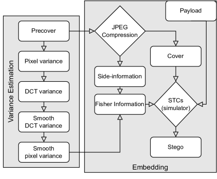
Figure 1: Embedding pipeline of JEEP. The Variance Estimation branch could be optionally replaced by a different methodology.

III-C Realistic Attacker

As mentioned in the previous section, full knowledge of the side information virtually disables its effect during embedding. In this section, we thus consider more realistic (even though still very powerful) Eve. In particular, we assume Eve has access to the variance of embedding changes $\mathrm{Var}(\eta)$ and the covariance between the embedding changes and the rounding errors $\mathrm{Cov}(\eta,U)$. On the other hand, we assume that Eve does not have access to the precover or the expectation of embedding change $\mathbb{E}[\eta]$. In practice, we are not sure if Eve can access the residuals $\mathbf{e}$, but it was shown [11] that the decompression rounding errors $\mathbf{y}-[\mathbf{y}]$ are excellent approximations of such signals. For this reason, we assume that Eve does, in fact, have access to the residuals. It is helpful to mention that with the knowledge we granted Eve, she cannot reconstruct the change rates $\beta_{kl}^{\pm}$ nor the side information $u_{kl}$. That is in accordance with our real-world expectations since the change rates are correlated with the side information, which is, by definition, inaccessible.

Eve’s hypothesis test then transforms into

$$\mathcal{H}_{0} : \mathbf{e}\sim\mathcal{N}(0,\Sigma_{ij}),$$ (41)

$$\mathcal{H}_{1} : \mathbf{e}\sim\mathcal{N}(0,\overline{\Sigma}_{ij}).$$ (42)

Following the same methodology from the previous section, we find that Alice wants to minimize the KL divergence (34), but the elements of the Fisher information matrix (35) are of the form

$$I_{kl}^{+} = (1-2u_{kl})^{4}I_{kl},$$ (43)

$$I_{kl}^{-} = (1+2u_{kl})^{4}I_{kl},$$ (44)

$$I_{kl}^{\pm} = (1+2u_{kl})^{2}(1-2u_{kl})^{2}I_{kl},$$ (45)

with $I_{kl}$ from (36).

The proposed strategy assumes that pixel variance is known to the steganographer. However, this is not the case in practice because Alice has an image and needs to estimate the variance in some way before the embedding procedure (unless we assume Alice has additional knowledge, which we do not in this work). Similarly, Eve, who observes a potential stego version of the same image, cannot know the actual variance of pixels. Since we want to compare two embedding strategies, assuming omniscient or realistic attacker, and we want to avoid the effect of imprecise variance estimation, we create an artificial source where we have control over pixel variances. This source is detailed in Section IV-A, and Section V-A shows that assuming omniscient Eve compared to the realistic one leads to severe security decay when tested against a state-of-the-art steganalyzer.

III-D Variance Estimation

In an image source where we do not know the variance of the noise, it is necessary to estimate it. However, this could create errors due to imprecise estimation. We will therefore use some of the best practices for estimating the variance. We consider two different variance estimators for two different situations. The first is for steganography targeting ’standard’ steganalysis, while the second targets the Reverse JPEG Compatibility Attack used for images compressed with QF 100.

III-D1 MiPOD-Estimator

For ’standard’ steganography, the methodology of computing variance, depicted in Figure 1, is described in the following. First, we need to estimate the pixel variances $\sigma_{ij}^{2}$. We decided to use a popular trigonometric variance estimator originally used for MiPOD [43], which is also used in its JPEG extension [19, 20]. For the sake of brevity, we refer the reader to the publications mentioned above for more details about the variance estimator.

Due to imprecise variance estimates, smoothing with the neighboring blocks in the DCT domain, as proposed in [20], is done to mitigate overly-content adaptive embedding. First, we compute the DCT variances $\Sigma_{kl}=\mathbf{D}\Sigma_{ij}\mathbf{D}^{T}$.

The squared variances are then smoothed by averaging nine neighboring DCT coefficients from the same DCT mode:

$$\tilde{\sigma}_{kl}^{-4}=\sum_{i=-1}^{1}\sum_{j=-1}^{1}w_{ij}\sigma_{k+8i,l+8j}^{-4},$$ (46)

where $\mathbf{w}$ is the averaging kernel:

$$\mathbf{w}=\frac{1}{20}\left(\begin{array}[]{ccc}1&3&1\\ 3&4&3\\ 1&3&1\end{array}\right).$$ (47)

Finally, the smooth DCT variances are lower-bounded by $\tilde{\sigma}_{kl}^{2}=\min\{10^{-10},\tilde{\sigma}_{kl}^{2}\}$, to prevent numerical instabilities, and decompressed to obtain final smoothed variance estimates $\tilde{\Sigma}_{ij}=\mathbf{D}^{T}\tilde{\Sigma}_{kl}\mathbf{D}$.

While we think there are many possible ways of smoothing the variance, we chose this (perhaps cumbersome) way because it has been shown in practice that smoothing the DCT variances provides good results for steganography.

Figure 2: Expectation of embedding change as a function of the rounding error $u_{kl}$ from one image, QF 95, 0.5 bpnzAC. Left: JEEP(o), right: JEEP(r).

III-D2 RJCA-Estimator

The second variance estimator we use in this work is for images compressed with QF 100. A different variance estimator is necessary because RJCA [11] can be used to steganalyze these images, and the MiPOD estimator was designed with feedback from spatial domain steganalysis. We decided to use constant variance for all pixels since it was shown [8] that using constant costs with a cleverly picked polarity of the embedding changes is a good strategy against the RJCA. We refer to JEEP with this constant variance estimator as JEEP-C. Unlike in the previous section, JEEP-C does not require Fisher Information smoothing. We also tested the MiPOD variance estimator for this case (JEEP); however, its performance was worse than using simple constant variance, and thus we do not mention its results.

III-E Obtaining the Change Rates

The goal of the proposed scheme is to solve (30) under the payload constraint (31). To achieve this, we use the method of Lagrange multipliers. Together with the payload constraint (31), this forms $2N+1$ equations with $2N+1$ unknowns composed of the change rates $\beta_{n}^{\pm},\,n=1,\ldots,N$, and the Lagrange multiplier $\vartheta$:

$$\beta_{n}^{+}I_{n}^{+}+\beta_{n}^{-}I_{n}^{\pm} = \lambda\log\frac{1-\beta_{n}^{+}-\beta_{n}^{-}}{\beta_{n}^{+}},$$ (48)

$$\beta_{n}^{-}I_{n}^{-}+\beta_{n}^{+}I_{n}^{\pm} = \lambda\log\frac{1-\beta_{n}^{+}-\beta_{n}^{-}}{\beta_{n}^{-}},$$ (49)

$$\sum_{n=1}^{N}H_{3}(\beta_{n}^{+},\beta_{n}^{-}) = \alpha.$$ (50)

Equations (48)-(50) can be solved efficiently with the Newton method by parallelizing over all $N$ DCT coefficients and a binary search over $\lambda$ satisfying the payload constraint.

To employ a coding mechanism, such as Syndrome-trellis codes [25], the change rates can be converted into embedding costs:

$$\rho_{n}^{\pm} = \log\left(\frac{1-\beta_{n}^{+}-\beta_{n}^{-}}{\beta_{n}^{\pm}}\right).$$ (51)

The costs are obtained by inverting the formula for optimal change rates, given embedding costs:

$$\beta_{n}^{\pm}=\frac{e^{-\lambda\rho_{n}^{\pm}}}{1+e^{-\lambda\rho_{n}^{+}}+e^{-\lambda\rho_{n}^{-}}}.$$ (52)

III-F Discussion

We observed that constraining embedding in the ’rational’ DCT modes, as described in Section I-A, is indeed necessary in order to avoid security deterioration. However, we can see that this would not be the case for omniscient Eve since then the term (37) needs to be present in the Fisher information, which automatically avoids the problem of Fisher information being zero.

It was shown [14] that steganographic costs can be viewed as estimators of a reciprocal standard deviation of pixels. Seeing the linear relationship between the standard deviation and the side information (43),(44) could explain why using the linear term $(1-2u_{kl})$ in the cost-based side-informed steganography (3),(4) works best in practice. Interestingly, a second power of $(1-2u_{kl})$ (5) was derived in [23] from the image model. We believe this is due to modeling stego image as a mixture of Gaussian distributions. The fourth power of $(1\pm 2u_{kl})$ present in (43),(44) was already used in SI-JMiPOD [20], but the explanation was heuristic and did not come from the image model. This heuristic also prevented the authors from using ternary embedding since they were probably unsure how to handle the term $I_{kl}^{\pm}$. Since JMiPOD models stego DCT coefficients as a Gaussian mixture, we believe the modulation (5) should have been used instead, similarly as in SI-MiPOD [23].

Lastly, if the side information is unavailable, JEEP naturally degenerates into a non-informed scheme, simply by setting $\mathbb{E}[u]=0$. Interestingly, even though the proposed method changes pixel variance instead of mean, the resulting Fisher information closely resembles that of JMiPOD. While JMiPOD computes DCT variance (11) and uses its square to compute the Fisher information $\sigma_{kl}^{-4}=\left(\sum_{i,j=0}^{7}\left(f_{kl}^{ij}\right)^{2}\sigma_{ij}^{2}\right)^{-2}$, we found out that the Fisher information contains $\sum_{i,j=0}^{7}\frac{\left(f_{kl}^{ij}\right)^{4}}{\sigma_{ij}^{4}}$ instead. It can be easily shown that the value computed by JMiPOD is always greater than $I_{kl}$, making the embedding more content-adaptive.

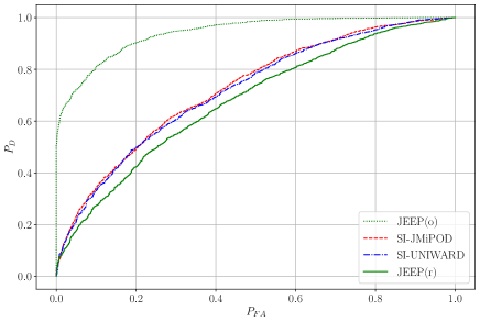
Figure 3: ROC curves of JIN-SRNet, trained on N-BOSSBase cover images compressed with QF 95 and stego images embedded with 0.5 bpnzAC.

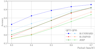
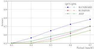
Figure 4: Accuracy of JIN-SRNet (left) and DCTR (right) for BOSSBase.

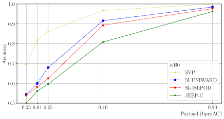
Figure 5: Accuracy of e-B0 for BOSSBase images compressed with QF 100.

IV Datasets and Detectors

To experimentally verify our results, we chose two popular datasets used for steganographic benchmarking. First is the BOSSbase [4] dataset, made of $10,000$ uncompressed grayscale images of size $512\times 512$, split into training, validation, and testing sets of sizes $7,000$, $1,000$, and $2,000$, respectively. The other dataset is the ALASKA2 dataset [18], comprising $25,000$ uncompressed grayscale images of size $512\times 512$. We split the ALASKA2 dataset into training, validation, and testing sets of $22,000$, $1,000$, and $2,000$ images. Both datasets are then JPEG compressed with python’s PIL library with several quality factors (QF). For security comparison with the prior art, we picked SI-UNIWARD [22, 37, 35] and SI-JMiPOD [20] algorithms as two main representatives of state-of-the-art steganography with side information. To add more contrast w.r.t. prior art on QF 100, we added SVP [8]. This algorithm was explicitly designed to be robust against the RJCA, even though without the use of side information.

We use three types of detectors to evaluate steganographic security. First is EfficientNet-B0 [41], initialized with weights pre-trained on the ImageNet dataset [24]. This detector, which we denote as e-B0, is used to test security against the RJCA and is trained only on the spatial domain rounding errors $e_{ij}=y_{ij}-[y_{ij}]$ of images compressed with QF 100. The second detector we use to verify security in the pixel domain is the JIN-SRNet [15], SRNet [5] pre-trained on ImageNet embedded with J-UNIWARD at a variable payload. The SRNet was trained with the Pair Constraint (PC) - forcing the cover and its stego version into the same mini-batch. Unlike in [15], it was observed in this work to boost the network’s performance. We believe this is caused by a much bigger security of the side-informed algorithms. The PC was not used for the e-B0, as it did not bring any detection improvements. Mini-batch size of both detectors was set to 32 images. The first detector is only trained for 15 epochs, as the detection saturates quickly in this scenario. The JIN-SRNet, on the other hand, is trained for 50 epochs in BOSSBase and 20 epochs in ALASKA2 due it its much bigger training set. Because the detectability in the spatial domain is typically much smaller than in the RJCA scenarios, we use larger payloads for the spatial domain detector. The last detector we use is the Low-Complexity Linear Classifier [21] (LCLC) coupled with DCTR features [36]. We include this detector to verify security in the DCT domain as well. The LCLC was trained on half of the images and tested on the other half for both datasets.

IV-A Controlled Source

To verify the validity of our assumptions on Eve’s knowledge, we created an artificial cover source [7], which allows us to have the true pixel variances without the need to estimate them. In this dataset, we denoise the images to eliminate the dependencies caused by the RAW development and further processing. The images are then noisified to enforce our cover model (14). We briefly summarize the creation of the dataset in 5 steps:

1) Estimate pixel variance $\sigma_{ij}^{2}$ using MiPOD’s variance estimator introduced in Section (III-D).

2) Denoise every image with Daubechies 8-tap wavelets [40] by removing i.i.d. Gaussian noise with a standard deviation $\sigma_{\mathrm{den}}=10$. The (non-integer) pixel values of the denoised image are clipped to the dynamic range of 8-bit grayscale images $[0,255]$.

3) Narrow the dynamic range into $[15,240]$ by a linear transformation of the pixels and round them to integers. Denote them as $\mu_{ij}$.

4) Adjust the variance so that the probability of a noisified pixel being outside of the interval $[0,255]$ is equal to a one-sided $5\sigma$ Gaussian outlier ($2.87\times 10^{-7}$). This is done by computing $\underline{\sigma}_{ij}=\min\{\frac{1}{5}\min\{\mu_{ij},255-\mu_{ij}\},\sigma_{ij}\}$.

5) Noisify cover pixels $x_{ij}$ by adding samples from $\mathcal{N}(0,\underline{\sigma}_{ij}^{2})$. The resulting cover image model comprises independent Gaussian variables $\mathcal{N}(x_{ij},\underline{\sigma}_{ij}^{2})$ rounded to the nearest integers and clipped to $[0,255]$.

For more details about the ’noisifying’ procedure, see [7]. This noisified dataset was created from BOSSbase, and we refer to it as N-BOSSbase.

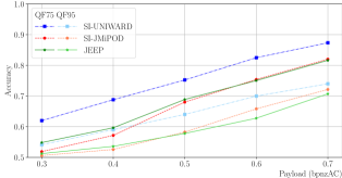
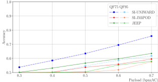
Figure 6: Accuracy of JIN-SRNet (left) and DCTR (right) for ALASKA2.

Figure 7: Accuracy of eB0 for ALASKA2 images compressed with QF 100.

V Results

In this section, we first evaluate the validity of assumptions on the steganalyst by training a detector in a controlled environment. We show that assuming all-powerful Eve is a fundamental mistake Alice can make because the detectability of her resulting embedding algorithm is extremely high. In the other two sections, we evaluate JEEP in BOSSBase and ALASKA2 datasets with several steganalyzers. We show that it provides superior security to previous state-of-the-art side-informed steganography.

V-A Attacker Capabilities Effect (Controlled Source)

In this section, we aim to investigate the difference between Alice’s assumptions on Eve. On the one hand, Eve is assumed to be omniscient - has full access to the side information. We have shown in Section III-B that Alice’s embedding strategy, in this case, is to minimize the KL divergence with the Fisher information matrix (38)-(40). On the other hand, Alice can assume a more realistic Eve described in Section III-C. The only thing Alice needs to change in such a scenario is using the Fisher information matrix of the form (43)-(45) instead. We refer to these two embedding algorithms as JEEP(o) and JEEP(r) for omniscient and realistic.

In Figure 2, we show the expectation of embedding change $\beta^{+}-\beta^{-}$ as a function of the rounding error $u$ for the omniscient and realistic attacker. We can clearly see that for the omniscient Eve, the side information has no effect on the embedding because it stays symmetric. For the realistic attacker, the side information introduces a lot of asymmetry.

Next, we trained JIN-SRNet on the denoised images from N-BOSSBase compressed with QF 95 and embedded with $0.5$ bits per non-zero AC DCT coefficient (bpnzAC). We used SI-JMiPOD, SI-UNIWARD, and JEEP(o,r). Since the pixel variances are known for all methods, we skipped the smoothing (46) (SI-UNIWARD does not use any smoothing). We show the ROC curves of these detectors in Figure 3. Several observations can be made from this figure. First, the assumption of omniscient Eve during embedding makes, in fact, makes the scheme highly detectable. Next, JEEP(r) provides the best security across embedding schemes. We believe the improvement over SI-JMiPOD comes mainly from two things. 1) JEEP is, by nature, a ternary embedding scheme, which reduces the total number of embedding changes. 2) Different methodology of computing the Fisher information aimed specifically against spatial steganalysis, as pointed out in Section III-F. And lastly, SI-JMiPOD and SI-UNIWARD have a very similar ROC curve, which is somewhat surprising because in uncontrolled datasets (see Sections V-B,V-C), SI-UNIWARD is way more detectable.

We have seen that with a state-of-the-art steganalyzer, assuming an omniscient attacker during embedding leads to severe security underperformance. That makes us conclude that such an assumption is unrealistic, and for the rest of the paper, we only assume realistic Eve. We will refer to Alice’s embedding algorithm simply as JEEP.

V-B BOSSBase

In this section, we evaluate the empirical security of JEEP in the popular BOSSBase database. In Figure 4, we plot the accuracies of SRNet and DCTR as a function of relative payload $\alpha$ for QFs 75 and 95. When steganalyzing with SRNet, we can see similar behavior for JEEP and SI-JMiPOD at QF 75, with SI-UNIWARD being much more detectable across all payloads. For QF 95, we can see better security for JEEP by up to 3.2% in terms of accuracy. With DCTR, we can see that JEEP is more detectable than SI-JMiPOD. That is not surprising, as JEEP was built with a decompressed image model, while JMiPOD uses a model in the DCT domain, where the steganalysis is performed. However, we can see that the detectability is much higher in the spatial domain across all QFs and payloads.

Results for images compressed with QF 100 are shown in Figure 5. Notice that the payloads are much smaller due to the detection power of RJCA. While JEEP is slightly more secure than SI-JMiPOD (results were omitted), we can see significant improvements in security with JEEP-C, up to 9% for 0.1 bpnzAC. Finally, compared to the state-of-the-art SVP without side information, we can see security gains of up to 27%.

V-C ALASKA2

Results for the ALASKA2 dataset are fairly similar to BOSSBase. We can still see better security of SI-JMiPOD against DCTR. However, SRNet is a more accurate detector, which in the end makes JEEP more secure. We can observe that for payloads below 0.5 bpnzAC, JEEP is a bit more detectable than SI-JMiPOD. We consider this difference statistically insignificant since the detectability of both schemes for these lower payloads is below 60%. In other cases, JEEP offers better security than the other two embedding schemes. This is especially true for QF 95, where JEEP outperforms SI-JMiPOD by up to 3% for 0.6 bpnzAC.

At QF 100, we again see improvement of JEEP-C over other side-informed methods by up to 5.5% in detectability at 0.1 bpnzAC. Compared to non-informed SVP, the gains are as high as 29.5%.

VI Conclusions

This paper introduces a side-informed embedding scheme driven by a statistical model of a decompressed image. For the first time, the side information, in the form of JPEG compression rounding errors, is used through covariance with the embedding changes. This allows us to get rid of typical heuristics around the rounding errors. Since we cannot compute the covariance from one given observation of a rounding error, we estimate its value with the help of several simplifying assumptions. This naturally creates an asymmetry of embedding changes, which is captured by the Fisher information matrix.

Due to better steganalysis in the spatial domain, we use this covariance in the model of a decompressed JPEG image. We then minimize the Kullback-Leibler divergence between the cover and stego distributions to bound the power of the likelihood ratio test. To be statistically significant, we show that the side information can be and has to be considered unavailable to a potential attacker.

We demonstrate through experiments that the proposed algorithm outperforms other state-of-the-art side-informed algorithms. This is especially true for images compressed with Quality Factor 100, where the Reverse JPEG Compatibility Attack can be applied. By using constant pixel variance, the gains in security are up to 9%. In the future, we plan to extend the methodology into color images, as well as different types of side information.

The source code for JEEP will be made available from https://janbutora.github.io/downloads/ upon acceptance of this paper.

Lemma 1.

If $\beta^{+}\geq 2\beta^{-},u\geq 0$, then

$$3(\beta^{+}-\beta^{-})u\geq 2(\beta^{+}+\beta^{-})u^{2}.$$

Similarly for $\beta^{-}\geq 2\beta^{+},u\leq 0$.

Proof:

For $u=0$, the result holds.

Let now $u\in(0,1/2]$ and $\beta^{+}\geq 2\beta^{-}$. Let us assume $3(\beta^{+}-\beta^{-})<2(\beta^{+}+\beta^{-})u$. We will show that this leads to a contradiction.

It follows that

$$\beta^{+}(3-2u) < \beta^{-}(2u+3)$$

$$\frac{\beta^{+}}{\beta^{-}} < \frac{2u+3}{3-2u}$$

$$= -1+\frac{6}{3-2u}$$

$$< 2.$$

∎

LIKELIHOOD-RATIO TEST

For clarity, we omit the indices of variables in the following. The test statistic of the LRT (25) for a single pixel is

$$\Lambda(e) = \frac{1}{2}\log\frac{\sigma^{2}}{\overline{\sigma}^{2}}+e^{2}\frac{\overline{\sigma}^{2}-\sigma^{2}}{2\sigma^{2}\overline{\sigma}^{2}}+e\frac{\mu}{\overline{\sigma}^{2}}-\frac{\mu^{2}}{2\overline{\sigma}^{2}}.$$

It follows that the mean of the test statistic under null and alternative hypotheses is

$$\mathbb{E}_{0}[\Lambda(e)] = \frac{1}{2}\log\frac{\sigma^{2}}{\overline{\sigma}^{2}}+\frac{\overline{\sigma}^{2}-\sigma^{2}}{2\overline{\sigma}^{2}}-\frac{\mu^{2}}{2\overline{\sigma}^{2}},$$

$$\mathbb{E}_{1}[\Lambda(e)] = \frac{1}{2}\log\frac{\sigma^{2}}{\overline{\sigma}^{2}}+\frac{\overline{\sigma}^{2}-\sigma^{2}}{2\sigma^{2}}+\mu^{2}\frac{2\sigma^{2}-\overline{\sigma}^{2}}{2\sigma^{2}\overline{\sigma}^{2}}.$$

Next, let us remind the reader that for a random variable $X\sim\mathcal{N}(\mu,\sigma^{2})$, the fourth moment is computed as $\mathbb{E}[X^{4}]=\mu^{4}+6\mu^{2}\sigma^{2}+3\sigma^{4}$, and variance of $X^{2}$ is then given by $\mathrm{Var}(X^{2})=\mathbb{E}[X^{4}]-\sigma^{4}-\mu^{4}-2\mu^{2}\sigma^{2}=2\sigma^{4}+4\mu^{2}\sigma^{2}.$

The variances of a pixel test statistic are

$$\mathrm{Var}_{0}[\Lambda(e)] = \frac{\sigma^{2}}{\overline{\sigma}^{2}}(\overline{\sigma}^{2}-\sigma^{2}+\mu),$$

$$\mathrm{Var}_{1}[\Lambda(e)] = \frac{\overline{\sigma}^{2}+2\mu^{2}}{\sigma^{2}}(\overline{\sigma}^{2}-\sigma^{2})+\mu.$$

The deflection coefficient $\delta$ and the variance effect $\varrho$ from (26) can now be expressed as

$$\delta = \frac{\sum_{i=1}^{N}\left(\mathbb{E}_{1}[\Lambda(e_{i})]-\mathbb{E}_{0}[\Lambda(e_{i})]\right)}{\sqrt{\sum_{i=1}^{N}\mathrm{Var}_{0}[\Lambda(e_{i})]}}$$

$$= \frac{\sum_{i=1}^{N}\frac{\left(\overline{\sigma}_{i}^{2}-\sigma_{i}^{2}\right)^{2}+\mu_{i}^{2}(3\sigma_{i}^{2}-\overline{\sigma}_{i}^{2})}{2\sigma_{i}^{2}\overline{\sigma}_{i}^{2}}}{\sqrt{\sum_{i=1}^{N}\frac{\sigma_{i}^{2}}{\overline{\sigma}_{i}^{2}}(\overline{\sigma}_{i}^{2}-\sigma_{i}^{2}+\mu_{i})}},$$

and

$$\varrho = \frac{\sum_{i=1}^{N}\mathrm{Var}_{1}[\Lambda(e_{i})]}{\sum_{i=1}^{N}\mathrm{Var}_{0}[\Lambda(e_{i})]}$$

$$= \frac{\sum_{i=1}^{N}\frac{\overline{\sigma}_{i}^{2}+2\mu_{i}^{2}}{\sigma_{i}^{2}}(\overline{\sigma}_{i}^{2}-\sigma_{i}^{2})+\mu_{i}}{\sum_{i=1}^{N}\frac{\sigma_{i}^{2}}{\overline{\sigma}_{i}^{2}}(\overline{\sigma}_{i}^{2}-\sigma_{i}^{2}+\mu_{i})}.$$

We can see that even for realistic Eve ($\boldsymbol{\mu}=\mathbf{0})$, expressions for $\delta$ and $\varrho$ are not possible to write down in a simple form.

TAYLOR EXPANSION OF KL DIVERGENCE

Denote $D(\boldsymbol{\beta})=D(C||S)$ the $8\times 8$ block KL divergence (33), where $\boldsymbol{\beta}$ is a vector of all 128 change rates $\beta_{kl}^{+},\beta_{kl}^{-},\,0\leq k,l\leq 7$. Using the independence of embedding changes (S1), the derivatives of stego mean and variance are

$$\frac{\partial\overline{\sigma}_{ij}^{2}}{\partial\beta_{kl}^{\pm}} = \left(f_{kl}^{ij}\right)^{2}q_{kl}^{2}((1\mp 2u_{kl})^{2}\mp 2(\beta_{kl}^{+}-\beta_{kl}^{-})),$$

$$\frac{\partial^{2}\overline{\sigma}_{ij}^{2}}{\partial^{2}\beta_{kl}^{\pm}} = -2\left(f_{kl}^{ij}\right)^{2}q_{kl}^{2},$$

$$\frac{\partial^{2}\overline{\sigma}_{ij}^{2}}{\partial\beta_{kl}^{+}\partial\beta_{kl}^{-}} = 2\left(f_{kl}^{ij}\right)^{2}q_{kl}^{2},$$

$$\frac{\partial\mu_{ij}}{\partial\beta_{kl}^{\pm}} = \pm f_{kl}^{ij}q_{kl}.$$

Second-order Taylor expansion around zero dictates $D(\boldsymbol{\beta})=D(\mathbf{0})+\boldsymbol{\beta}\nabla D(\mathbf{0})+\frac{1}{2}\boldsymbol{\beta}\nabla^{2}D(0)\boldsymbol{\beta}^{T}.$

For zero-change rates, the stego distribution is equal to the cover distribution, therefore $D(\mathbf{0})=0$. The derivatives of the KL divergence w.r.t. change rates are

$$\frac{\partial}{\partial\beta_{kl}^{\pm}}D(\boldsymbol{\beta}) = \frac{\partial}{\partial\beta_{kl}^{\pm}}\frac{1}{2}\sum_{i,j=0}^{7}\log\frac{\overline{\sigma}_{ij}^{2}}{\sigma_{ij}^{2}}+\frac{\mu_{ij}^{2}+\sigma_{ij}^{2}-\overline{\sigma}_{ij}^{2}}{\overline{\sigma}_{ij}^{2}}$$

$$= \frac{1}{2}\sum_{i,j=0}^{7}\left(\frac{\partial\overline{\sigma}_{ij}^{2}/\partial\beta_{kl}^{\pm}}{\overline{\sigma}_{ij}^{2}}-\frac{\sigma_{ij}^{2}\partial\overline{\sigma}_{ij}^{2}/\partial\beta_{kl}^{\pm}}{\overline{\sigma}_{ij}^{4}}\right.$$

$$\left.+\frac{2\mu_{ij}\overline{\sigma}_{ij}^{2}\partial\mu_{ij}/\partial\beta_{kl}^{\pm}-\mu_{ij}^{2}\partial\overline{\sigma}_{ij}^{2}/\partial\beta_{kl}^{\pm}}{\overline{\sigma}_{ij}^{4}}\right).$$

Then, since $\overline{\sigma}_{ij}^{2}|_{\boldsymbol{\beta}=\mathbf{0}}=\sigma_{ij}^{2}$ we get $\nabla D(\mathbf{0})=\mathbf{0}$. We already see that the only remaining term in the Taylor expansion is the Fisher information matrix. We will show only the computation of $I_{kl}^{+}$ since $I_{kl}^{-}$ and $I_{kl}^{\pm}$ follow the same logic.

Denoting $\partial\overline{\sigma}_{ij}^{2}=\partial\overline{\sigma}_{ij}^{2}/\partial\beta_{kl}^{+}$, $\partial^{2}\overline{\sigma}_{ij}^{2}=\partial^{2}\overline{\sigma}_{ij}^{2}/\partial^{2}\beta_{kl}^{+}$ and $\partial\mu_{ij}=\partial\mu_{ij}/\partial\beta_{kl}^{+}$, the second derivative of KL divergence is

$$\frac{\partial^{2}}{\partial^{2}\beta_{kl}^{+}}D(\boldsymbol{\beta}) = \frac{1}{2}\sum_{i,j}\left(\frac{\overline{\sigma}_{ij}^{2}\partial^{2}\overline{\sigma}_{ij}^{2}-(\partial\overline{\sigma}_{ij}^{2})^{2}}{\overline{\sigma}_{ij}^{4}}\right.$$

$$+\frac{2\overline{\sigma}_{ij}^{2}(\partial\mu_{ij})^{2}-\mu_{ij}^{2}\partial^{2}\overline{\sigma}_{ij}^{2}}{\overline{\sigma}_{ij}^{4}}$$

$$-\frac{\sigma_{ij}^{2}\overline{\sigma}_{ij}^{4}\partial^{2}\overline{\sigma}_{ij}^{2}-2\overline{\sigma}_{ij}^{2}\sigma_{ij}^{2}(\partial\overline{\sigma}_{ij}^{2})^{2}}{\overline{\sigma}_{ij}^{8}}$$

$$\left.-\frac{2\overline{\sigma}_{ij}^{2}\partial\overline{\sigma}_{ij}^{2}(2\mu_{ij}\overline{\sigma}_{ij}^{2}\partial\mu_{ij}-\mu_{ij}^{2}\partial\overline{\sigma}_{ij}^{2})}{\overline{\sigma}_{ij}^{8}}\right).$$

Finally

$$I_{kl}^{+} = \frac{\partial^{2}}{\partial^{2}\beta_{kl}^{+}}D(\mathbf{0})$$

$$= \frac{1}{2}\sum_{i,j=0}^{7}\frac{(\partial\overline{\sigma}_{ij}^{2}|_{\boldsymbol{\beta}=\mathbf{0}})^{2}}{\sigma_{ij}^{4}}+2\frac{(\partial\mu_{ij})^{2}}{\sigma_{ij}^{2}}$$

$$= \frac{1}{2}\sum_{i,j=0}^{7}\frac{\left(f_{kl}^{ij}\right)^{4}q_{kl}^{4}(1-2u_{kl})^{4}}{\sigma_{ij}^{4}}+2\frac{\left(f_{kl}^{ij}\right)^{2}q_{kl}^{2}}{\sigma_{ij}^{2}}.$$

References

- [1] S. Agarwal and H. Farid. Photo forensics from JPEG dimples. In IEEE Workshop on Information Forensics and Security (WIFS), December 4-7, 2017.
- [2] P. Bas. Steganography via cover-source switching. In 2016 IEEE International Workshop on Information Forensics and Security (WIFS), pages 1–6, 2016.
- [3] P. Bas. An embedding mechanism for natural steganography after down-sampling. In 2017 IEEE International Conference on Acoustics, Speech and Signal Processing (ICASSP), pages 2127–2131, 2017.
- [4] P. Bas, T. Filler, and T. Pevný. Break our steganographic system – the ins and outs of organizing BOSS. In T. Filler, T. Pevný, A. Ker, and S. Craver, editors, Information Hiding, 13th International Conference, volume 6958 of Lecture Notes in Computer Science, pages 59–70, Prague, Czech Republic, May 18–20, 2011.
- [5] M. Boroumand, M. Chen, and J. Fridrich. Deep residual network for steganalysis of digital images. IEEE Transactions on Information Forensics and Security, 14(5):1181–1193, May 2019.
- [6] M. Boroumand and J. Fridrich. Synchronizing embedding changes in side-informed steganography. In Proceedings IS&T, Electronic Imaging, Media Watermarking, Security, and Forensics 2020, San Francisco, CA, January 26–30 2020.
- [7] M. Boroumand, J. Fridrich, and R. Cogranne. Are we there yet? In A. Alattar and N. D. Memon, editors, Proceedings IS&T, Electronic Imaging, Media Watermarking, Security, and Forensics 2019, San Francisco, CA, January 14–17, 2019.
- [8] J. Butora and P. Bas. Fighting the reverse jpeg compatibility attack: Pick your side. In The 10th ACM Workshop on Information Hiding and Multimedia Security, Santa Barbara, CA, June 27–28, 2022.
- [9] J. Butora and J. Fridrich. Detection of diversified stego sources using CNNs. In A. Alattar and N. D. Memon, editors, Proceedings IS&T, Electronic Imaging, Media Watermarking, Security, and Forensics 2019, San Francisco, CA, January 14–17, 2019.
- [10] J. Butora and J. Fridrich. Minimum perturbation cost modulation for side-informed steganography. In A. Alattar, N. D. Memon, and G. Sharma, editors, Proceedings IS&T, Electronic Imaging, Media Watermarking, Security, and Forensics 2020, San Francisco, CA, January 26–30, 2020.
- [11] J. Butora and J. Fridrich. Reverse JPEG compatibility attack. IEEE Transactions on Information Forensics and Security, 15:1444–1454, 2020.
- [12] J. Butora and J. Fridrich. Steganography and its detection in JPEG images obtained with the "trunc" quantizer. In Proceedings IEEE, International Conference on Acoustics, Speech, and Signal Processing, Barcelona, Spain, May 4–8, 2020.
- [13] J. Butora and J. Fridrich. Revisiting perturbed quantization. In The 9th ACM Workshop on Information Hiding and Multimedia Security, Brussels, Belgium, June 21–25, 2021.
- [14] J. Butora, Y. Yousfi, and J. Fridrich. Turning cost-based steganography into model-based. In C. Riess and F. Schirrmacher, editors, The 8th ACM Workshop on Information Hiding and Multimedia Security, Denver, CO, June 22–25, 2020. ACM Press.
- [15] J. Butora, Y. Yousfi, and J. Fridrich. How to pretrain for steganalysis. In The 9th ACM Workshop on Information Hiding and Multimedia Security, Brussels, Belgium, June 21–25, 2021.
- [16] K. Chubachi. An ensemble model using CNNs on different domains for ALASKA2 image steganalysis. In IEEE International Workshop on Information Forensics and Security, New York, NY, December 6–11, 2020.
- [17] R. Cogranne. Selection-channel-aware reverse JPEG compatibility for highly reliable steganalysis of JPEG images. In Proceedings IEEE, International Conference on Acoustics, Speech, and Signal Processing, pages 2772–2776, Barcelona, Spain, May 4–8, 2020.
- [18] R. Cogranne, Q. Giboulot, and P. Bas. ALASKA–2: Challenging academic research on steganalysis with realistic images. In IEEE International Workshop on Information Forensics and Security, New York, NY, December 6–11, 2020.
- [19] R. Cogranne, Q. Giboulot, and P. Bas. Steganography by minimizing statistical detectability: The cases of jpeg and color images. In C. Riess and F. Schirrmacher, editors, The 8th ACM Workshop on Information Hiding and Multimedia Security, Denver, CO, 2020. ACM Press.
- [20] R. Cogranne, Q. Giboulot, and P. Bas. Efficient steganography in jpeg images by minimizing performance of optimal detector. IEEE Transactions on Information Forensics and Security, 17:1328–1343, 2022.
- [21] R. Cogranne, V. Sedighi, T. Pevný, and J. Fridrich. Is ensemble classifier needed for steganalysis in high-dimensional feature spaces? In IEEE International Workshop on Information Forensics and Security, Rome, Italy, November 16–19, 2015.
- [22] T. Denemark and J. Fridrich. Side-informed steganography with additive distortion. In IEEE International Workshop on Information Forensics and Security, Rome, Italy, November 16–19 2015.
- [23] T. Denemark and J. Fridrich. Model based steganography with precover. In A. Alattar and N. D. Memon, editors, Proceedings IS&T, Electronic Imaging, Media Watermarking, Security, and Forensics 2017, San Francisco, CA, January 29–February 1, 2017.
- [24] J. Deng, W. Dong, R. Socher, L. Li, K. Li, and L. Fei-Fei. ImageNet: A large-scale hierarchical image database. In IEEE conference on computer vision and pattern recognition, pages 248–255, June 20–25, 2009.
- [25] T. Filler, J. Judas, and J. Fridrich. Minimizing additive distortion in steganography using syndrome-trellis codes. IEEE Transactions on Information Forensics and Security, 6(3):920–935, September 2011.
- [26] J. Fridrich. On the role of side-information in steganography in empirical covers. In A. Alattar, N. D. Memon, and C. Heitzenrater, editors, Proceedings SPIE, Electronic Imaging, Media Watermarking, Security, and Forensics 2013, volume 8665, pages 1–11, San Francisco, CA, February 5–7, 2013.
- [27] J. Fridrich, M. Goljan, and D. Soukal. Perturbed quantization steganography. ACM Multimedia System Journal, 11(2):98–107, 2005.
- [28] Q. Giboulot, P. Bas, and R. Cogranne. Multivariate side-informed gaussian embedding minimizing statistical detectability. IEEE Transactions on Information Forensics and Security, 17:1841–1854, 2022.
- [29] Q. Giboulot, R. Cogranne, and P. Bas. JPEG steganography with side information from the processing pipeline. In Proceedings IEEE, International Conference on Acoustics, Speech, and Signal Processing, pages 2767–2771, Barcelona, Spain, May 4–8, 2020.
- [30] Q. Giboulot, R. Cogranne, and P. Bas. Synchronization Minimizing Statistical Detectability for Side-Informed JPEG Steganography. In IEEE International Workshop on Information Forensics and Security, New York, NY, December 6–11, 2020.
- [31] L. Guo, J. Ni, and Y.-Q. Shi. An efficient JPEG steganographic scheme using uniform embedding. In Fourth IEEE International Workshop on Information Forensics and Security, Tenerife, Spain, December 2–5, 2012.
- [32] L. Guo, J. Ni, and Y. Q. Shi. Uniform embedding for efficient JPEG steganography. IEEE Transactions on Information Forensics and Security, 9(5):814–825, May 2014.
- [33] L. Guo, J. Ni, W. Su, C. Tang, and Y. Shi. Using statistical image model for JPEG steganography: Uniform embedding revisited. IEEE Transactions on Information Forensics and Security, 10(12):2669–2680, 2015.
- [34] V. Holub and J. Fridrich. Designing steganographic distortion using directional filters. In Fourth IEEE International Workshop on Information Forensics and Security, Tenerife, Spain, December 2–5, 2012.
- [35] V. Holub and J. Fridrich. Digital image steganography using universal distortion. In W. Puech, M. Chaumont, J. Dittmann, and P. Campisi, editors, 1st ACM IH&MMSec. Workshop, Montpellier, France, June 17–19, 2013.
- [36] V. Holub and J. Fridrich. Low-complexity features for JPEG steganalysis using undecimated DCT. IEEE Transactions on Information Forensics and Security, 10(2):219–228, February 2015.
- [37] V. Holub, J. Fridrich, and T. Denemark. Universal distortion design for steganography in an arbitrary domain. EURASIP Journal on Information Security, Special Issue on Revised Selected Papers of the 1st ACM IH and MMS Workshop, 2014:1, 2014.
- [38] E.L. Lehmann and J.P. Romano. Testing Statistical Hypotheses, Second Edition. Springer, 3rd edition, 2005.
- [39] B. Li, M. Wang, and J. Huang. A new cost function for spatial image steganography. In Proceedings IEEE, International Conference on Image Processing, ICIP, Paris, France, October 27–30, 2014.
- [40] M. K. Mihcak, I. Kozintsev, K. Ramchandran, and P. Moulin. Low-complexity image denoising based on statistical modeling of wavelet coefficients. IEEE Signal Processing Letters, 6(12):300–303, December 1999.
- [41] T. Mingxing and V. L. Quoc. EfficientNet: Rethinking model scaling for convolutional neural networks. In Proceedings of the 36th International Conference on Machine Learning, ICML, volume 97, pages 6105–6114, June 9–15, 2019.
- [42] W. Pennebaker and J. Mitchell. JPEG: Still Image Data Compression Standard. Van Nostrand Reinhold, New York, 1993.
- [43] V. Sedighi, R. Cogranne, and J. Fridrich. Content-adaptive steganography by minimizing statistical detectability. IEEE Transactions on Information Forensics and Security, 11(2):221–234, 2015.
- [44] T. Taburet, P. Bas, W. Sawaya, and J. Fridrich. A natural steganography embedding scheme dedicated to color sensors in the JPEG domain. In A. Alattar and N. D. Memon, editors, Proceedings IS&T, Electronic Imaging, Media Watermarking, Security, and Forensics 2019, San Francisco, CA, January 14–17, 2019.
- [45] T. Taburet, P. Bas, W. Sawaya, and J. Fridrich. Natural steganography in jpeg domain with a linear development pipeline. IEEE Transactions on Information Forensics and Security, 16:173–186, 2021.
- [46] Y. Yousfi, J. Butora, J. Fridrich, and C. F. Tsang. Improving EfficientNet for JPEG steganalysis. In The 9th ACM Workshop on Information Hiding and Multimedia Security, Brussels, Belgium, June 21–25, 2021.
- [47] Y. Yousfi, J. Butora, Q. Giboulot, and J. Fridrich. Breaking ALASKA: Color separation for steganalysis in JPEG domain. In R. Cogranne and L. Verdoliva, editors, The 7th ACM Workshop on Information Hiding and Multimedia Security, Paris, France, July 3–5, 2019. ACM Press.
- [48] Y. Yousfi, J. Butora, E. Khvedchenya, and J. Fridrich. Imagenet pre-trained cnns for jpeg steganalysis. In IEEE International Workshop on Information Forensics and Security, New York, NY, December 6–11, 2020.