Phenomenological description of the $\pi^{-}\pi^{+}$ $S$-waves in $D^{+}\to\pi^{-}\pi^{+}\pi^{+}$ and $D^{+}_{s}\to\pi^{-}\pi^{+}\pi^{+}$ decays: The problem of phases.

Abstract

We present a phenomenological description of the LHCb data for the magnitudes and phases of the $\pi^{-}\pi^{+}$ $S$-wave amplitudes in the $D^{+}\to\pi^{-}\pi^{+}\pi^{+}$ and $D^{+}_{s}\to\pi^{-}\pi^{+}\pi^{+}$ decays. We operate within a simple model that takes into account the known pair interactions of particles in coupled channels. The seed complex amplitudes for various intermediate state production are assumed to be independent of the energy; their values are determined by fitting. This model gives a satisfactory description of virtually all features of the energy dependence of the experimentally measured $S$-wave amplitudes in the $D^{+}\to\pi^{-}\pi^{+}\pi^{+}$ and $D^{+}_{s}\to\pi^{-}\pi^{+}\pi^{+}$ decays in the regions $2m_{\pi}<m_{\pi^{-}\pi^{+}}<1.39\mbox{ GeV}$ and $2m_{\pi}<m_{\pi^{-}\pi^{+}}<1.29\mbox{ GeV}$, respectively.

I Introduction

Measurements of three-body decays of $D$- and $D_{s}$-mesons into $\pi^{-}\pi^{+}\pi^{+}$, $K^{-}\pi^{+}\pi^{+}$, $K^{+}K^{-}\pi^{+}$, $K^{-}K^{+}K^{+}$, etc. Aa22 ; Ai01a ; Ai01 ; Li04 ; Bo07 ; Bo08 ; Au09 ; Sa11 ; No15 ; Re16 ; Aa19 ; Ab21 ; Aa22a ; Ze22 ; PDG22 represent the most important extension of the classical studies of three-pion decays of strange mesons $K\to\pi\pi\pi$ Am22 ; PDG22 into a family of charmed pseudoscalar states. Information about the resonant structures in the two-body mass spectra in these decays is obtained from the Dalitz plot fits using the isobar model Aa22 ; Ai01a ; Ai01 ; Li04 ; Bo07 ; Bo08 ; Au09 ; Sa11 ; No15 ; Re16 ; Aa19 ; Ab21 ; Aa22a ; Ze22 ; PDG22 and quasimodel-independent partial wave analysis Aa22 ; Aa22a ; Ai01 ; Bo08 ; Au09 ; Ab21 ; Re16 . Further, we will speak about the $D^{+}\to\pi^{-}\pi^{+}\pi^{+}$ and $D^{+}_{s}\to\pi^{-}\pi^{+}\pi^{+}$ decays for which the LHCb Collaboration has recently obtained the detailed high-statistics data Aa22 ; Aa22a . For the data analysis, the amplitude of the $D^{+}\to\pi^{-}\pi^{+}\pi^{+}$ decay Aa22 was approximated by the coherent sum (symmetrized with respect to the permutation of two identical pions) of the $S$-wave contribution and higher-spin waves (the same approximation was also used for the amplitude of the $D^{+}_{s}\to\pi^{-}\pi^{+}\pi^{+}$ decay Aa22a ),

$$\mathcal{A}(s_{12},s_{13})=\left[\mathcal{A}_{S{\scriptsize\mbox{-wave}}}(s_{12})+\sum_{i}a_{i}e^{i\delta_{i}}\mathcal{A}_{i}(s_{12},s_{13})\right]+(s_{12}\leftrightarrow s_{13}),$$ (1)

where $s_{12}=(p_{1}+p_{2})^{2}$ and $s_{13}=(p_{1}+p_{3})^{2}$ are the squares of the invariant masses of two different $\pi^{-}\pi^{+}$ pairs ($\pi^{-}_{1}\pi^{+}_{2}$ and $\pi^{-}_{1}\pi^{+}_{3}$); $p_{1}$, $p_{2}$, $p_{3}$ are the four-momenta of the final pions. The first term in square brackets is the $S$-wave amplitude,

$$\mathcal{A}_{S{\scriptsize\mbox{-wave}}}(s_{12})=a_{0}(s_{12})e^{i\delta_{0}(s_{12})}.$$ (2)

The values of the real functions $a_{0}(s_{12})$ and $\delta_{0}(s_{12})$ were obtained by the Dalitz plot fitting for 50 intervals (knots) into which the accessible region of $\sqrt{s_{12}}\equiv m_{\pi^{-}\pi^{+}}$ ($2m_{\pi}<m_{\pi^{-}\pi^{+}}<m_{D(D_{s})}-m_{\pi}$) was divided Aa22 ; Aa22a . This technique allows one to obtain information about the $\pi^{-}\pi^{+}$ $S$-waves in the $D^{+}\to\pi^{-}\pi^{+}\pi^{+}$ and $D^{+}_{s}\to\pi^{-}\pi^{+}\pi^{+}$ decays without any model assumptions about their composition [i.e., about the contributions of the states $f_{0}(500)$, $f_{0}(980)$, $f_{0}(1370)$, $f_{0}(1500)$, etc.]. The motivation for applying this method is the presence of overlapping wide and narrow light scalar resonances in the region below 2 GeV with poorly-known masses and widths. The LHCb data on the $S$-wave amplitudes in the $D^{+}\to\pi^{-}\pi^{+}\pi^{+}$ Aa22 and $D^{+}_{s}\to\pi^{-}\pi^{+}\pi^{+}$ Aa22a decays are shown below in Figs. 3 and 4. The $S$-wave contributions in these decays are dominant. They account for approximately 62% and 85% of the full decay rate of $D^{+}$ and $D^{+}_{s}$ into $\pi^{-}\pi^{+}\pi^{+}$, respectively. In turn, the amplitudes of the $P$- and $D$-waves, represented by the terms in the sum in Eq. (1), were approximated in the isobar model by the contributions of the known resonances $\rho^{0}(770)$, $\omega(782)$, $\rho^{0}(1450)$, $\rho^{0}(1700)$, $f_{2}(1270)$, and $f^{\prime}_{2}(1525)$. The amplitude $\mathcal{A}_{i}(s_{12},s_{13})$ of resonance $R_{i}$ includes the Breit-Wigner complex resonant amplitude, angular distribution, and Blatt-Weiskopf barrier factors (for more details of the parametrization see Refs. Aa22 ; Aa22a ). The magnitude and phase of the $R_{i}$ production amplitude, $a_{i}$ and $\delta_{i}$, are free (independent of $s_{12}$ and $s_{13}$) parameters within the isobar model. Their values relative to the magnitude and phase of the amplitude of the selected reference subprocess (which are taken to be 1 and 0^∘, respectively) were also determined in Refs. Aa22 ; Aa22a from the fits to the data.

The data on the values and energy dependence of the phases of the $S$-waves in the $\pi^{-}\pi^{+}$ channel obtained from the $D^{+}\to\pi^{-}\pi^{+}\pi^{+}$ and $D^{+}_{s}\to\pi^{-}\pi^{+}\pi^{+}$ decays and $\pi^{+}\pi^{-}\to\pi^{+}\pi^{-}$ reaction are discussed in detail and compared with each other in Ref. Aa22a . Obvious differences between all three phases indicate deviations from the Watson final-state interaction theorem Wa52 in the $D^{+}\to\pi^{-}\pi^{+}\pi^{+}$ and $D^{+}_{s}\to\pi^{-}\pi^{+}\pi^{+}$ decays. This fact is also evidence of the important role of intermediate multibody hadronic interactions (multiquark fluctuations) on the formation of the phases of the production amplitudes of final two-body subsystems in these and related decays (for example, in $D^{+}\to K^{-}\pi^{+}\pi^{+}$) Aa22a ; Ro11 ; Fr14 ; Ro15 ; No15 ; Re16 ; Lo16 ; Wa22 . In general, the problem of explaining the specific values of the phases $\delta_{i}$ included in Eq. (1) and the energy dependence of the $S$-wave phases $\delta_{0}(s_{12})$ seems to be key for elucidation of the mechanisms of the $D^{+}\to\pi^{-}\pi^{+}\pi^{+}$ and $D^{+}_{s}\to\pi^{-}\pi^{+}\pi^{+}$ decays.

This paper presents a phenomenological description of the LHCb data for the magnitudes and phases of the $S$-wave amplitudes of the $\pi^{-}\pi^{+}$ systems produced in the $D^{+}\to\pi^{-}\pi^{+}\pi^{+}$ and $D^{+}_{s}\to\pi^{-}\pi^{+}\pi^{+}$ decays. Our model is described in Sec. II. The fittings to the data on $S$ waves in the decays of $D$ and $D_{s}$ mesons are presented in Secs. III and IV, respectively. Predictions for the $\pi^{0}\pi^{0}$ $S$-waves in the $D^{+}\to\pi^{+}\pi^{0}\pi^{0}$ and $D^{+}_{s}\to\pi^{+}\pi^{0}\pi^{0}$ decays are made in Sec. V. The results of our analysis are briefly formulated in Sec. VI.

II A phenomenological model for the $S$-waves

As is well known, light scalar mesons are richly produced in the reactions $\pi^{+}\pi^{-}\to\pi^{+}\pi^{-}$ and $\pi^{+}\pi^{-}\to K\bar{K}$, information about which is extracted from the more complicated peripheral processes $\pi^{\pm}N\to[(\pi\pi),(K\bar{K})](N,\Delta)$ dominated by the one-pion exchange mechanism. We will assume that in the processes in which the initial state is not the $\pi\pi$ scattering state, the light scalar mesons $f_{0}(500)$ and $f_{0}(980)$ are produced in interactions of intermediate pseudoscalar mesons $\pi^{+}$ with $\pi^{-}$, $\pi^{0}$ with $\pi^{0}$, and $K$ with $\bar{K}$. Note that such a mechanism is quite consistent with the hypothesis of a four-quark ($q^{2}\bar{q}^{2}$) nature of light scalars Ja77 ; Ac89 ; Ac98 ; Ac03a . The scheme of their formation in the $D^{+}\to\pi^{-}\pi^{+}\pi^{+}$ and $D^{+}_{s}\to\pi^{-}\pi^{+}\pi^{+}$ decays is graphically represented in Fig. 1. At the first step, the valence $c$-quark decays into light quarks, the initial states of the $D^{+}=c\bar{d}$ and $D^{+}_{s}=c\bar{s}$ mesons “boil up”, passing into a mixture of various quark-gluon fluctuations, which are then combined into pions, kaons, etc. The latter can additionally enter into pair interactions with each other in the final state. We take into account the seed three-body $S$-wave fluctuations $D^{+}/D^{+}_{s}\to\pi^{+}\pi^{+}\pi^{-}$, $D^{+}/D^{+}_{s}\to\pi^{+}\pi^{0}\pi^{0}$, $D^{+}/D^{+}_{s}\to\pi^{+}K^{+}K^{-}$, and $D^{+}/D^{+}_{s}\to\pi^{+}K^{0}\bar{K}^{0}$ (the corresponding amplitudes are shown in Fig. 1 by thick black dots). In so doing, the $f_{0}(500)-f_{0}(980)$ resonance complex is produced as a result of $\pi\pi$ and $K\bar{K}$ interactions in the final state. The amplitudes corresponding to these subprocesses are indicated in Fig. 1 as $T_{ab\to\pi^{+}\pi^{-}}$, where $ab=\pi^{+}\pi^{-}$, $\pi^{0}\pi^{0}$, $K^{+}K^{-}$, $K^{0}\bar{K}^{0}$.

Figure 1: The $f_{0}(500)-f_{0}(980)$ resonance complex production amplitude in the $D^{+}\to\pi^{-}\pi^{+}\pi^{+}$ and $D^{+}_{s}\to\pi^{-}\pi^{+}\pi^{+}$ decays. Contributions of the intermediate states $ab=\pi^{+}\pi^{-}$, $\pi^{0}\pi^{0}$, $K^{+}K^{-}$, $K^{0}\bar{K}^{0}$ are summed.

According to this figure, we write the $S$-wave amplitude $\mathcal{A}_{S{\scriptsize\mbox{-wave}}}(s_{12})=a_{0}(s_{12})e^{i\delta_{0}(s_{12})}$ for the $D^{+}/D^{+}_{s}\to\pi^{-}\pi^{+}\pi^{+}$ decay (taking into account the renaming $s_{12}\equiv s\equiv m^{2}_{\pi^{-}\pi^{+}}$) in the following form

$${\mathcal{A}_{S\scriptsize\mbox{-wave}}(s)=a_{0}(s)e^{i\delta_{0}(s)}}=\lambda_{\pi^{+}\pi^{-}}+\sum_{ab}\lambda_{ab}I_{ab}(s)\xi_{ab}\,T_{ab\to\pi^{+}\pi^{-}}(s),$$ (3)

where $\xi_{ab}=1/2$ for $ab=\pi^{0}\pi^{0}$ and $=1$ in other cases; $T_{\pi^{+}\pi^{-}\to\pi^{+}\pi^{-}}(s)=\frac{2}{3}T^{0}_{0}(s)+\frac{1}{3}T^{2}_{0}(s)$, $T_{\pi^{0}\pi^{0}\to\pi^{+}\pi^{-}}(s)=\frac{2}{3}[T^{0}_{0}(s)-T^{2}_{0}(s)]$, where $T^{0}_{0}(s)$ and $T^{2}_{0}(s)$ are the $S$-amplitudes of the reaction $\pi\pi\to\pi\pi$ in the channels with isospin $I=0$ and 2, respectively, $T^{I}_{0}(s)=[\eta^{I}_{0}(s)\exp(2i\delta^{I}_{0}(s))-1]/(2i\rho_{\pi\pi}(s))$, where $\eta^{I}_{0}(s)$ and $\delta^{I}_{0}(s)$ are the corresponding inelasticity and phase of $\pi\pi$ scattering ($\eta^{0}_{0}(s)=1$ at $s<4m^{2}_{K^{+}}$, and $\eta^{2}_{0}(s)=1$ in the whole region of $s$ under consideration), $\rho_{\pi\pi}(s)=\sqrt{1-4m^{2}_{\pi}/s}$. For the $S$-wave transition amplitudes $K\bar{K}\to\pi\pi$ we have $T_{K^{+}K^{-}\to\pi^{+}\pi^{-}}(s)=T_{K^{0}\bar{K}^{0}\to\pi^{+}\pi^{-}}(s)$ and $T_{K\bar{K}\to\pi\pi}(s)=T_{\pi\pi\to K\bar{K}}(s)$. The function $I_{ab}(s)$ is the amplitude of the $ab$ loop. Above the $ab$ threshold, $I_{ab}(s)$ has the form

$$I_{ab}(s)=C_{ab}+\rho_{ab}(s)\left(i-\frac{1}{\pi}\ln\frac{1+\rho_{ab}(s)}{1-\rho_{ab}(s)}\right),$$ (4)

where $\rho_{ab}(s)=\sqrt{1-4m^{2}_{a}/s}$ (we put $m_{\pi^{+}}=m_{\pi^{0}}\equiv m_{\pi}$ and take into account the mass difference of $K^{+}$ and $K^{0}$) if $\sqrt{s}<2m_{K}$, then $\rho_{K\bar{K}}(s)\to i|\rho_{K\bar{K}}(s)|$, and $C_{ab}$ is a real subtraction constant in the $ab$ loop. $C_{\pi^{+}\pi^{-}}=C_{\pi^{0}\pi^{0}}\equiv C_{\pi\pi}$, $C_{K^{+}K^{-}}=C_{K^{0}\bar{K}^{0}}\equiv C_{K\bar{K}}$, and $I_{\pi^{+}\pi^{-}}(s)=I_{\pi^{0}\pi^{0}}(s)\equiv I_{\pi\pi}(s)$.

The seed $S$-wave amplitudes $\lambda_{ab}$ in Eq. (3) are approximated by complex constants. They are free parameters of the model along with the constants $C_{ab}$. A similar model approach has already been applied to the decays $D^{+}\to\pi^{-}\pi^{+}\pi^{+}$ Bo07 , $D/D_{s}\to\pi^{+}\pi^{-}e^{+}\nu_{e}$ Ac20 , and $J/\psi\to\gamma\pi^{0}\pi^{0}$ Ac21 . In fact, we are dealing with the description of the data on the $S$-wave components of $D^{+}/D^{+}_{s}\to\pi^{-}\pi^{+}\pi^{+}$ decays in the spirit of the isobar model in which instead of the resonant Breit-Wigner distributions one uses the known amplitudes $T^{0}_{0}(s)$, $T^{2}_{0}(s)$, and $T_{\pi\pi\to K\bar{K}}(s)$. All nontrivial dependence on $s$ is introduced into $\mathcal{A}_{S\scriptsize\mbox{-wave}}(s)$ by these amplitudes. In their meaning, the absolute values and phases of the amplitudes $\lambda_{ab}$ in Eq. (3) do not differ from the amplitudes $a_{i}$ and phases $\delta_{i}$ included in Eq. (1). In the isobar model, all these quantities are considered constant because they depend only on the total energy of the system, i.e., $m_{\pi^{-}\pi^{+}\pi^{+}}=\sqrt{(p_{1}+p_{2}+p_{3})^{2}}=M_{D/D_{s}}$ in our case, and do not depend on the subenergy $m_{\pi^{-}\pi^{+}}$. In particular, the imaginary parts of $\lambda_{ab}$ are understood as a result of the three-body final state interactions dressed the $c$ quark weak-decay vertices. Their presence due to the real and quasireal intermediate states that can appear at $m_{\pi^{-}\pi^{+}\pi^{+}}=M_{D/D_{s}}$ in the input channel. It is the complex amplitudes of the formation of resonances $a_{i}e^{i\delta_{i}}$ and the amplitudes $\lambda_{ab}$ that, within the framework of the isobar model, keep in mind the information about three-body interactions with participation of the spectator pion FN1 . The detailed discussion of the crucial approximations of the isobar model can be found, for example, in Refs. Re16 ; As85 ; Al93 ; Be11 ; Be20 . As noted in Ref. Aa22 , at present, there are no tools for a complete description of the amplitudes for thee-body decays from first principles. Recently, essential progress in the theoretical description of three-body decays is associated with dispersion methods, see, for example, Refs. Am22 ; Ro11 ; Fr14 ; Ro15 ; Gi64 ; Ca06 ; Ku12 ; Ku15 ; Al20 ; Al22 ; Ku22 and references therein. This approach, in principle, allows one to go beyond the phenomenological isobar model. In particular, it demonstrates that final-state interactions involving all three particles in hadronic loops turn out to be important sources of deviations from the Watson theorem. However, one cannot but recognize the complexity of applying dispersion methods Am22 ; Ro11 ; Fr14 ; Ro15 ; Ku12 ; Ku15 ; Al20 ; Al22 ; Ku22 for practical processing of the data on various three-body decays in comparison with the isobar model (see especially Refs. Am22 ; Ku22 ).

The mechanisms of formation of the seed amplitudes $\lambda_{\pi^{+}\pi^{-}}$ and $\lambda_{\pi^{0}\pi^{0}}$ in the general case can differ from each other, as well as the mechanisms of formation of $\lambda_{K^{+}K^{-}}$ and $\lambda_{K^{0}\bar{K}^{0}}$. If we take advantage of the language of quark diagrams, then, for example, due to the $D^{+}$ decay mechanism indicated in Fig. 2, only a $K^{0}\bar{K}^{0}$ pair can be produced, while $K^{+}K^{-}$ cannot. Therefore, no isotopic relations between the seed amplitudes of the different charge state production are assumed in advance.

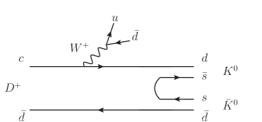
Figure 2: The tree-level external $W^{+}$-emission diagram leading to the $K^{0}\bar{K}^{0}$ pair production in the $D^{+}$ decay.

We take the amplitudes $T^{0}_{0}(s)$ and $T_{K\bar{K}\to\pi\pi}(s)=T_{\pi\pi\to K\bar{K}}(s)$ from Ref. Ac06 (corresponding to fitting variant 1 for parameters from Table 1 therein) containing the excellent simultaneous descriptions of the phase shifts, inelasticity, and mass distributions in the reactions $\pi\pi\to\pi\pi$, $\pi\pi\to K\bar{K}$, and $\phi\to\pi^{0}\pi^{0}\gamma$ (see also Refs. Ac11 ; Ac12 ). The amplitudes $T^{0}_{0}(s)$ and $T_{\pi\pi\to K\bar{K}}(s)$ were described in Refs. Ac06 ; Ac11 ; Ac12 by the complex of the mixed $f_{0}(500)$ and $f_{0}(980)$ resonances and smooth background contributions. The amplitude $T^{2}_{0}(s)$ is taken from Ref. Ac03 (see also Ref. Ac98a ).

III Description of the $D^{+}\to\pi^{-}\pi^{+}\pi^{+}$ data

Let us rewrite Eq. (3) in terms of the amplitudes $T^{0}_{0}(s)$, $T^{2}_{0}(s)$ and $T_{K^{+}K^{-}\to\pi^{+}\pi^{-}}(s)$ in the following form

$${\mathcal{A}_{S\scriptsize\mbox{-wave}}(s)=a_{0}(s)e^{i\delta_{0}(s)}}=\lambda_{\pi^{+}\pi^{-}}+I_{\pi\pi}(s)\left[T^{0}_{0}(s)\left(\frac{2}{3}\lambda_{\pi^{+}\pi^{-}}+\frac{1}{3}\lambda_{\pi^{0}\pi^{0}}\right)+T^{2}_{0}(s)\frac{1}{3}\left(\lambda_{\pi^{+}\pi^{-}}-\lambda_{\pi^{0}\pi^{0}}\right)\right]$$

$$+\left[\lambda_{K^{+}K^{-}}I_{K^{+}K^{-}}(s)+\lambda_{K^{0}\bar{K}^{0}}I_{K^{0}\bar{K}^{0}}(s)\right]T_{K^{+}K^{-}\to\pi^{+}\pi^{-}}(s).\qquad\quad\ \ \,$$ (5)

Note that if all $\lambda_{ab}$ are real and $\lambda_{\pi^{+}\pi^{-}}=\lambda_{\pi^{0}\pi^{0}}$ [i.e., the contribution of the amplitude $T^{2}_{0}(s)$ is absent], then the attempt to describe the data Aa22 about the phase $\delta_{0}(s)$ shown in Fig. 3(b) will fail. Really, in this case the phase $\delta_{0}(s)$ of the amplitude $\mathcal{A}_{S\scriptsize\mbox{-wave}}(s)$ [taking into account Eq. (4)] coincides with the $\pi\pi$ scattering phase $\delta^{0}_{0}(s)$ below the $K^{+}K^{-}$ threshold where $\eta^{0}_{0}(s)=1$ [as is the phase of the amplitude $T_{K^{+}K^{-}\to\pi^{0}\pi^{0}}(s)$ Ac06 ]. The phase $\delta^{0}_{0}(s)$ is shown in Fig. 3(b) by the dotted curve. We also note that in the vicinity of the $\pi\pi$ threshold, the phase $\delta_{0}(s)$ is approximately equal to $100^{\circ}$ [see Fig. 3(b)], and this cannot be described by any real constants $\lambda_{ab}$, since the phases $\delta^{0}_{0}(s)$ and $\delta^{2}_{0}(s)$ vanish at the $\pi\pi$ threshold and are small in its vicinity as is seen from Fig. 3(b).

Let us first consider the fitting variant in which the contribution of the amplitude $T_{K^{+}K^{-}\to\pi^{+}\pi^{-}}(s)$ is absent, i.e., $\lambda_{K^{+}K^{-}}=\lambda_{K^{0}\bar{K}^{0}}=0$. In this case, the connection with the $K\bar{K}$-channel is taken into account to the extent that it is present in the amplitude $T^{0}_{0}(s)$. This fitting variant is shown in Fig. 3 by the dashed curves. It corresponds to the following parameter values:

$$\lambda_{\pi^{+}\pi^{-}}=-1.72+i11.30,\ \ \lambda_{\pi^{0}\pi^{0}}=17.86+i6.59,\ \ C_{\pi\pi}=0.77.$$ (6)

The dash-dotted line in Fig. 3(a) shows the contribution caused by the amplitude $T^{2}_{0}(s)$. Surprisingly, this simple variant quite satisfactorily describes the observed features of the energy dependences of the magnitude and phase of the $S$-wave amplitude in the $D^{+}\to\pi^{-}\pi^{+}\pi^{+}$ decay in the region $2m_{\pi}<m_{\pi^{-}\pi^{+}}<1.39\mbox{ GeV}$.

Figure 3: The points with the error bars are the LHCb data Aa22 on the (a) magnitude $a_{0}$ and (b) phase $\delta_{0}$ of the $\pi^{-}\pi^{+}$ $S$-wave amplitude in the $D^{+}\to\pi^{-}\pi^{+}\pi^{+}$ decay. The statistical, experimental systematic, and model systematic uncertainties are added in quadrature. The solid curves represent our fit. The corresponding contribution to $a_{0}$ from the $T_{K^{+}K^{-}\to\pi^{+}\pi^{-}}$ amplitude in Eq. (III) is shown in plot (a) by the dotted curve. The dashed curves show the fit variant at $\lambda_{K^{+}K^{-}}=\lambda_{K^{0}\bar{K}^{0}}=0$. For this variant, the dash-dot curve in plot (a) shows the contribution from the $T^{2}_{0}$ amplitude. The vertical dotted lines show the fitting region boundary. In plot (b), the dotted curves show the $\pi\pi$ scattering $S$-wave phase shifts $\delta^{0}_{0}$ and $\delta^{2}_{0}$ which describe the corresponding data for the reactions $\pi^{+}\pi^{\mp}\to\pi^{+}\pi^{\mp}$ well.

The solid curves in Fig. 3 correspond to the fit without any restrictions on the values of the parameters $\lambda_{ab}$ in Eq. (III) (including $\lambda_{K^{+}K^{-}}$ and $\lambda_{K^{0}\bar{K}^{0}}$). Formally, this fit (with $\chi^{2}=162$) turns out to be noticeably better than the previous variant (with $\chi^{2}=278$). The values of the fitting parameters are the following:

$$\lambda_{\pi^{+}\pi^{-}}=-1.21+i11.21,\ \ \lambda_{\pi^{0}\pi^{0}}=20.40+i4.47,\ \ C_{\pi\pi}=0.68,\ \ \,$$

$$\lambda_{K^{+}K^{-}}=39.11+i27.43,\ \ \lambda_{K^{0}\bar{K}^{0}}=-32.93-i29.98,\ \ C_{K\bar{K}}=0.46.$$ (7)

The corresponding contribution to $a_{0}(s)$ from the amplitude $T_{K^{+}K^{-}\to\pi^{+}\pi^{-}}(s)$ is shown in Fig. 3(a) by the dotted curve. It should be noted that the solid curves and dashed curves for $a_{0}(s)$ and $\delta_{0}(s)$ presented in Fig. 3 are generally similar to each other.

Interestingly, the amplitude $a_{0}(s)$ [module of $\mathcal{A}_{S\scriptsize\mbox{-wave}}(s)$] reaches its minimum at $\sqrt{s}=m_{\pi^{-}\pi^{+}}\approx 0.9$ GeV [see Fig 3(a)], i.e., in the region where the amplitude of $\pi\pi$-scattering $T^{0}_{0}(s)$ reaches the unitary limit. On the contrary, the $f_{0}(980)$-resonance manifests itself in $|T^{0}_{0}(s)|$ as a deep and narrow dip, and in $a_{0}(s)$ it manifests itself as a resonance peak. By virtue of chiral symmetry, the resonance $f_{0}(500)$ (also known as $\sigma$) is shielded by the background in the $T^{0}_{0}(s)$ amplitude Ac94 ; Ac07 . Such a chiral suppression, as can be seen from Fig. 3(a) is absent in the $a_{0}(s)$ amplitude. As for the phase $\delta_{0}(s)$, its comparison with the $\pi\pi$ scattering phase $\delta^{0}_{0}(s)$ [see Fig. 3(b)] explicitly demonstrates a deviation from Watson’s theorem Wa52 , caused by the difference in the production mechanisms of the $S$-wave $\pi^{-}\pi^{+}$ system in the $D^{+}\to\pi^{-}\pi^{+}\pi^{+}$ decay and in $\pi\pi$-scattering.

When describing the peak near 1 GeV in Fig. 3(a), there is no double counting. Let us extract from the amplitude $\mathcal{A}_{S\scriptsize\mbox{-wave}}(s)$ in Eq. (3) the contribution with isospin $I=0$ caused by the creation of the $\pi\pi$ states. In the form suitable below the $K^{+}K^{-}$ threshold, this contribution is

$$\mathcal{A}^{0}_{0}(s)=\left(\frac{2}{3}\lambda_{\pi^{+}\pi^{-}}+\frac{1}{3}\lambda_{\pi^{0}\pi^{0}}\right)e^{i\delta^{0}_{0}(s)}\left[\cos\delta^{0}_{0}(s)+(\mbox{Re}I_{\pi\pi}(s))\sin\delta^{0}_{0}(s)\right].$$ (8)

As paradoxical as it may appear at first glance, just the dip in the amplitude $T^{0}_{0}(s)=e^{i\delta^{0}_{0}(s)}\sin\delta^{0}_{0}(s)/\rho_{\pi\pi}(s)$ in the $f_{0}(980)$ region (where the phase $\delta^{0}_{0}(s)$ changes very rapidly and passes through 180^∘) leads to a prominent peak in the $|\mathcal{A}^{0}_{0}(s)|$ near 1 GeV. The contribution of the $T_{K^{+}K^{-}\to\pi^{+}\pi^{-}}(s)$ amplitude [see the dotted curve in Fig. 3(a)] improves slightly the description of the peak. It is important to emphasize that these two sources of the peak in the $a_{0}(s)$ near 1 GeV have essentially different origins.

To describe the oscillations observed in $a_{0}(s)$ and $\delta_{0}(s)$ in the region of $m_{\pi^{-}\pi^{+}}>1.39$ GeV (see Fig. 3), additional considerations are needed about the possible mechanisms production of the $f_{0}(1370)$ and $f_{0}(1500)$ resonances. Their admixture (probably small) can enter into $\mathcal{A}_{S\scriptsize\mbox{-wave}}(s)$ through the $\pi\pi$-scattering amplitude $T^{0}_{0}(s)$. But the $f_{0}(1370)$ and $f_{0}(1500)$, being presumably $q\bar{q}$-states, may well be directly produced in the $D^{+}\to\pi^{-}\pi^{+}\pi^{+}$ decay. In this case, the corresponding contributions can be described phenomenologically within the framework of the usual isobar model. In this paper, we do not dwell on the description of the $m_{\pi^{-}\pi^{+}}>1.39$ GeV region, but we hope to do so elsewhere.

IV Description of the $D^{+}_{s}\to\pi^{-}\pi^{+}\pi^{+}$ data

Figure 4 shows the LHCb data Aa22a for the magnitude $a_{0}(s)$ and phase $\delta_{0}(s)$ of the $\pi^{-}\pi^{+}$ $S$-wave amplitude in the $D^{+}_{s}\to\pi^{-}\pi^{+}\pi^{+}$ decay. Let us note that the values given in Aa22a for the phase $\delta_{0}(s)$ are shifted in Fig. 4 by $+180^{\circ}$. This is done for the convenience of the comparison of all three phases $\delta_{0}(s)$, $\delta^{0}_{0}(s)$, and $\delta^{2}_{0}(s)$. The minus sign appearing in Eq. (3) as a result of this shift is absorbed in the coefficients $\lambda_{ab}$. The solid curves in Fig. 4, which quite successfully describe the data in the region $2m_{\pi}<m_{\pi^{-}\pi^{+}}<1.29\mbox{ GeV}$, correspond to a very simple variant of the model. This variant is suggested by the very data on the $D^{+}_{s}\to\pi^{-}\pi^{+}\pi^{+}$ decay and by the experience obtained with describing $a_{0}(s)$ and $\delta_{0}(s)$ for the $D^{+}\to\pi^{-}\pi^{+}\pi^{+}$ decay. Here we focus on this variant only.

Figure 4: The points with the error bars are the LHCb data Aa22a on the (a) magnitude $a_{0}$ and (b) phase $\delta_{0}$ of the $\pi^{-}\pi^{+}$ $S$-wave amplitude in the $D^{+}_{s}\to\pi^{-}\pi^{+}\pi^{+}$ decay. The statistical, experimental systematic, and model systematic uncertainties are added in quadrature. The solid curves represent our fit. The dashed curve in plot (a) shows the contribution to $a_{0}$ caused by the term proportional to $\lambda_{\pi^{+}\pi^{-}}$ in Eq. (9). The vertical dotted lines show the fitting region boundary. In plot (b), the dotted curves show the $\pi\pi$ scattering $S$-wave phase shifts $\delta^{0}_{0}$ and $\delta^{2}_{0}$ well describing the corresponding data for the reactions $\pi^{+}\pi^{\mp}\to\pi^{+}\pi^{\mp}$.

When passing from the description of the $D^{+}$ decay to the description of the $D^{+}_{s}$ decay, we do not change the notations of the parameters $\lambda_{ab}$ and $C_{ab}$. We put in Eq. (III) $\lambda_{\pi^{0}\pi^{0}}=-2\lambda_{\pi^{+}\pi^{-}}$ [which means the suppression of the contribution of the amplitude $T^{0}_{0}(s)$] and $\lambda_{K^{+}K^{-}}=\lambda_{K^{0}\bar{K}^{0}}$ [in terms of quark diagrams, this equality holds, for example, for the seed mechanism with external radiation of the $W^{+}$ boson $D^{+}_{c}(c\bar{s})\to W^{+}s\bar{s}\to\pi^{+}(K^{+}K^{-}+K^{0}\bar{K}^{0})$]. Thus, we obtain

$${\mathcal{A}_{S\scriptsize\mbox{-wave}}(s)=a_{0}(s)e^{i\delta_{0}(s)}}=\lambda_{\pi^{+}\pi^{-}}[1+I_{\pi\pi}(s)T^{2}_{0}(s)]+\lambda_{K^{+}K^{-}}\left[I_{K^{+}K^{-}}(s)+I_{K^{0}\bar{K}^{0}}(s)\right]T_{K^{+}K^{-}\to\pi^{+}\pi^{-}}(s).$$ (9)

The solid curves in Fig. 4 demonstrate the result of the fitting to the data using Eq. (9). The parameter values for this fit (with $\chi^{2}=129$) are the following:

$$\lambda_{\pi^{+}\pi^{-}}=5.37-i2.30,\ \ C_{\pi\pi}=1.69,\ \ \lambda_{K^{+}K^{-}}=20.18-i8.94,\ \ C_{K\bar{K}}=0.60.$$ (10)

In this case, it is almost obvious how each of the contributions works. In $a_{0}(s)$ [see Fig. 4(a)], the region of the $f_{0}(980)$ resonance is dominated by the contribution of the amplitude $T_{K^{+}K^{-}\to\pi^{+}\pi^{-}}(s)$. In the region $m_{\pi^{-}\pi^{+}}<0.9$ GeV, the contribution of the $f_{0}(980)$ rapidly falls, and $a_{0}(s)$ is dominated by the weakly energy-dependent contribution proportional to $\lambda_{\pi^{+}\pi^{-}}$ in Eq. (9). The phase of this contribution is small, smooth, and negative, like the $\delta^{2}_{0}(s)$ phase [see Fig. 4(b)]. As $m_{\pi^{-}\pi^{+}}$ increases, it is compensated due to the rapidly increasing positive phase of the amplitude $T_{K^{+}K^{-}\to\pi^{+}\pi^{-}}(s)$ [see Fig. 4(b)], which, below the $K^{+}K^{-}$-threshold, coincides with $\pi\pi$-scattering phase shift $\delta^{0}_{0}(s)$ Ac06 . As $m_{\pi^{-}\pi^{+}}$ increases further, the description of the $\delta_{0}(s)$ phase remains quite successful up to $m_{\pi^{-}\pi^{+}}\approx 1.29$ GeV. About the description of the data in the region of the $f_{0}(1370)$ and $f_{0}(1500)$ resonances, we can only repeat what has been said at the end of the previous section.

V Predictions for the $D^{+}$ and $D^{+}_{s}$ decays into $\pi^{+}\pi^{0}\pi^{0}$

For the $S$-wave amplitude of the $\pi^{0}\pi^{0}$-system produced in the decay $D^{+}\to\pi^{+}\pi^{0}\pi^{0}$ we have

$${\mathcal{A}_{S\scriptsize\mbox{-wave}}(s)=a_{0}(s)e^{i\delta_{0}(s)}}=\lambda_{\pi^{0}\pi^{0}}+I_{\pi\pi}(s)\left[T^{0}_{0}(s)\left(\frac{2}{3}\lambda_{\pi^{+}\pi^{-}}+\frac{1}{3}\lambda_{\pi^{0}\pi^{0}}\right)-T^{2}_{0}(s)\frac{2}{3}\left(\lambda_{\pi^{+}\pi^{-}}-\lambda_{\pi^{0}\pi^{0}}\right)\right]$$

$$+\left[\lambda_{K^{+}K^{-}}I_{K^{+}K^{-}}(s)+\lambda_{K^{0}\bar{K}^{0}}I_{K^{0}\bar{K}^{0}}(s)\right]T_{K^{+}K^{-}\to\pi^{0}\pi^{0}}(s),\qquad\quad\ \ \,$$ (11)

where $T_{K^{+}K^{-}\to\pi^{0}\pi^{0}}(s)=T_{K^{+}K^{-}\to\pi^{+}\pi^{-}}(s)$. The curves for $a_{0}(s)$ and $\delta_{0}(s)$ shown in Fig. 5 are obtained using Eq. (V) after substituting into it the parameter values from Eq. (III).

Figure 5: Predictions for the (a) magnitude $a_{0}$ and (b) phase $\delta_{0}$ of the $\pi^{0}\pi^{0}$ $S$-wave amplitude in $D^{+}\to\pi^{+}\pi^{0}\pi^{0}$.

An analog of Eq. (9) for the $D^{+}_{s}\to\pi^{+}\pi^{0}\pi^{0}$ decay has the form

$${\mathcal{A}_{S\scriptsize\mbox{-wave}}(s)=a_{0}(s)e^{i\delta_{0}(s)}}=\lambda_{\pi^{0}\pi^{0}}[1+I_{\pi\pi}(s)T^{2}_{0}(s)]+\lambda_{K^{+}K^{-}}\left[I_{K^{+}K^{-}}(s)+I_{K^{0}\bar{K}^{0}}(s)\right]T_{K^{+}K^{-}\to\pi^{0}\pi^{0}}(s),$$ (12)

where $T_{K^{+}K^{-}\to\pi^{0}\pi^{0}}(s)=T_{K^{+}K^{-}\to\pi^{+}\pi^{-}}(s)$ and $\lambda_{\pi^{0}\pi^{0}}=-2\lambda_{\pi^{+}\pi^{-}}$. The curves for $a_{0}(s)$ and $\delta_{0}(s)$ shown in Fig. 6 are obtained using Eq. (12) after substituting into it the parameter values from Eq. (10).

Figure 6: Predictions for the (a) magnitude $a_{0}$ and (b) phase $\delta_{0}$ of the $\pi^{0}\pi^{0}$ $S$-wave amplitude in $D^{+}_{s}\to\pi^{+}\pi^{0}\pi^{0}$.

Comparison of the curves in Figs. 5 and 6 with the corresponding curves in Figs. 3 and 4 reveals that the predictions obtained for the decays $D^{+}\to\pi^{+}\pi^{0}\pi^{0}$ and $D^{+}_{s}\to\pi^{+}\pi^{0}\pi^{0}$ are crucial to the verification of the presented phenomenological model.

VI Conclusion

To describe the amplitudes of the $S$-wave three-pion decays of the $D^{+}$ and $D^{+}_{s}$ mesons, a phenomenological model is presented in which the production of the light scalar mesons $f_{0}(500)$ and $f_{0}(980)$ occurs due to $\pi\pi$ and $K\bar{K}$ interactions in the final state. Such a production mechanism is consistent with the hypothesis of the four-quark nature of the $f_{0}(500)$ and $f_{0}(980)$ states. Using this model, it is possible to satisfactorily describe virtually all features of the energy dependence of the $\pi^{-}\pi^{+}$ $S$-wave amplitudes measured in the $D^{+}\to\pi^{-}\pi^{+}\pi^{+}$ and $D^{+}_{s}\to\pi^{-}\pi^{+}\pi^{+}$ decays in the regions $2m_{\pi}<m_{\pi^{-}\pi^{+}}<1.39\mbox{ GeV}$ and $2m_{\pi}<m_{\pi^{-}\pi^{+}}<1.29\mbox{ GeV}$, respectively. The model predictions are presented for the $D^{+}\to\pi^{+}\pi^{0}\pi^{0}$ and $D^{+}_{s}\to\pi^{+}\pi^{0}\pi^{0}$ decays. Their verification will be very critical for our model. A problem common to all isobar models with the explanation of the phases of the meson pair production amplitudes in multibody weak hadronic decays of charm states is noted.

The $S$-wave phases measured using the quasimodel-independent partial wave analysis Aa22 ; Aa22a ; Ai01 ; Bo08 ; Au09 ; Ab21 ; Re16 contain valuable information about the contributions associated with three-body interactions. But even if the phases of the $ab$ scattering are known, as for the $\pi\pi$ and $K\pi$ systems, to separate the contributions from the different isospin amplitudes it is necessary to additionally use a model (for example, of the type used by us). It can be hoped that for the $ab$ channels with a definite isospin, the difference between the $S$-wave phase obtained from $ab$ scattering data and the phase found from the three-body decay is reduced simply to an overall relative shift, at least in the elastic region [see, for example, Eq. (8)]. For example, in this way one can determine the phase of $\pi\eta$ scattering up to an additive constant. Thus, it would be very interesting to perform the quasimodel-independent partial wave analysis of high-statistics data on the $D^{+}_{s}\to\pi^{+}\pi^{0}\eta$ decay, in which the $\pi^{+}\eta$ and $\pi^{0}\eta$ $S$-wave amplitudes are parametrized as complex functions determined from the fitting to the data. It is natural that the found amplitudes can be compared with theoretical predictions for the elastic $\pi\eta$ scattering.

ACKNOWLEDGMENTS

The work was carried out within the framework of the state contract of the Sobolev Institute of Mathematics, Project No. FWNF-2022-0021.

References

- (1) R. L. Workman et al. (Particle Data Group), Review of particle physics, Prog. Theor. Exp. Phys. 2022, 083C01 (2022).
- (2) E. M. Aitala et al. (E791 Collaboration), Study of the Decay and Measurement of Masses and Widths, Phys. Rev. Lett. 86, 765 (2001).
- (3) E. M. Aitala et al. (E791 Collaboration), Experimental Evidence for a Light and Broad Scalar Resonance in Decay, Phys. Rev. Lett. 86, 770 (2001).
- (4) J. M. Link et al. (FOCUS Collaboration), Dalitz plot analysis of and decay to using the K-matrix formalism, Phys. Lett. B 585, 200 (2004).
- (5) G. Bonvicini et al. (CLEO Collaboration), Dalitz plot analisis of the decay, Phys. Rev. D 76, 012001 (2007).
- (6) G. Bonvicini et al. (CLEO Collaboration), Dalitz plot analysis of the decay, Phys. Rev. D 78, 052001 (2008).
- (7) B. Aubert et al. (BABAR Collaboration), Dalitz plot analysis of , Phys. Rev. D 79, 032003 (2009).
- (8) P. del Amo Sanchez et al. (BABAR Collaboration), Dalitz plot analysis of , Phys. Rev. D 83, 052001 (2011).
- (9) J. H. Alvarenga Nogueira et al., Summary of the 2015 LHCb workshop on multi-body decays of D and B mesons, arXiv:1605.03889.
- (10) Alberto C. dos Reis, LHCb — three-body decays of charged mesons, Sec. IV, p. 13 in arXiv:1605.03889.
- (11) R. Aaij et al. (LHCb Collaboration), Dalitz plot analysis of the decay , J. High Energy Phys. 04 (2019) 063.
- (12) M. Ablikim et al. (BESIII Collaboration), Amplitude analysis of the decay, Phys. Rev. 106, 112006 (2022).
- (13) X. Zeng, Hadronic decays at BESIII, in Proceedings of the 13th International Workshop on collisions from Phi to Psi (Fudan University, Shanghai, China, 2022).
- (14) R. Aaij et al. (LHCb Collaboration), Amplitude analysis of the decay and measurement of the S-wave amplitude, arXiv:2208.03300.
- (15) R. Aaij et al. (LHCb Collaboration), Amplitude analysis of the decay, arXiv:2209.09840.
- (16) G. D’Ambrosio1, M. Knecht, and S. Neshatpour, Determination of the structure of the amplitudes from recent data, Phys. Lett. B 835, 137594 (2022).
- (17) K. M. Watson, Phys. Rev. 88, 1163 (1952).
- (18) P. C. Magalhães, M. R. Robilotta, K. S. F. F. Guimarães, T. Frederico, W. de Paula, I. Bediaga, A. C. dos Reis, C. M. Maekawa, and G. R. S. Zarnauskas, Towards three-body unitarity in , Phys. Rev. D 84, 094001 (2011).
- (19) K. S. F. F. Guimarães, O. Lourenço, W. de Paula, T. Frederico, A. C. dos Reis, Final state interaction in with I=1/2 and 3/2 channels, J. High Energy Phys. 08 (2014) 135.
- (20) P. C. Magalhães and M. R. Robilotta, - the weak vector current, Phys. Rev. D 92, 094005 (2015).
- (21) B. Loiseau, Theory overview on amplitude analyses with charm decays, Proc. Sci. CHARM2016 (2016) 033 [arXiv:1611.05286].
- (22) Z. Y. Wang, H. A. Ahmed, and C. W. Xiao, Scalar resonances in the final state interactions of the decays , , , Phys. Rev. D 105, 016030 (2022).
- (23) R. L. Jaffe, Multiquark hadrons. I. Phenomenology of mesons, Phys. Rev. D 15, 267 (1977); Multiquark hadrons. II. Methods, 15, 281 (1977).
- (24) N. N. Achasov and V. N. Ivanchenko, On a search for four-quark states in radiative decays of mesons, Nucl. Phys. B315, 465 (1989).
- (25) N. N. Achasov, On the nature of the and scalar mesons, Usp. Fiz. Nauk 168, 1257 (1998) [Phys. Usp. 41, 1149 (1998)].
- (26) N. N. Achasov, Radiative decays of -meson about nature of light scalar resonances, Nucl. Phys. A728, 425 (2003).
- (27) N. N. Achasov, A. V. Kiselev, and G. N. Shestakov, Semileptonic decays and as the probe of constituent quark-antiquark pairs in the light scalar mesons, Phys. Rev. D 102, 016022 (2020).
- (28) N. N. Achasov, J. V. Bennett, A. V. Kiselev, E. A. Kozyrev, and G. N. Shestakov, Evidence of the four-quark nature of and , Phys. Rev. D 103, 014010 (2021), arXiv:2009.04191.
- (29) The amplitudes [see Eq. (3) and Fig. 1] in the isobar model formally resemble the amplitudes of contact interactions. However, they are not reduced to the amplitudes of tree point-like diagrams. These amplitudes are the sources of the production of non-resonant pairs. The amplitudes are intricately formed complex quantities including, among other things, projections of the production amplitudes of the resonances in the crossed channels onto the -wave channels and also inelastic sources of the production of states.
- (30) D. Aston, T. A. Lasinski, and P. K. Sinervo, The SLAC three-body partial wave analysis system, SLAC-Report-297, 1985.
- (31) H. Albrecht et al. (ARGUS Collaboration), A partial wave analysis of the decay , Phys. Lett. B 308, 435 (1993).
- (32) I. Bediaga, Heavy meson three body decay: Three decades of Dalitz plot amplitude analysis, arXiv:1104.0694.
- (33) I. Bediaga and C. Göbel, Direct CP violation in beauty and charm hadron decays, Prog. Part. Nucl. Phys. 114, 103808 (2020).
- (34) J. Gillespie, Final-state interactions, Holden-Day Advanced Physics Monographs, edited by Kennet M. Watson (Holden-Day, Inc., San Francisco, 1964).
- (35) I. Caprini, Rescattering effects and the pole in hadronic decays, Phys. Lett. B 638, 468 (2006).
- (36) F. Niecknig, B. Kubis, and S. P. Schneider, Dispersive analysis of and decays, Eur. Phys. J. C 72, 2014 (2012).
- (37) F. Niecknig and B. Kubis, Dispersion-theoretical analysis of the Dalitz plot, J. High Energy Phys. 10 (2015) 142.
- (38) M. Albaladejo, I. Danilkin, S. Gonzàlez-Solis, D. Winneyc, C.Fernández-Ramíreze, A. N. Hiller Blin, V. Mathieu, M. Mikhasenko, A. Pilloni, and A. Szczepaniak, and transition form factor revisited, Eur. Phys. J. C 80, 1107 542 (2020).
- (39) M. Albaladejo et al. (JPAC Collaboration), Novel approaches in hadron spectroscopy, Prog. Part. Nucl. Phys. 127, 103981 (2022).
- (40) D. Stamen, T. Isken, B. Kubis, M. Mikhasenko, and M. Niehus, Analysis of rescattering effects in final states, arXiv:2212.11767.
- (41) N. N. Achasov and A. V. Kiselev, Properties of the light scalar mesons face the experimental data on the decay and the scattering, Phys. Rev. D 73, 054029 (2006).
- (42) N. N. Achasov and A. V. Kiselev, Analytical scattering amplitude and the light scalars, Phys. Rev. D 83, 054008 (2011).
- (43) N. N. Achasov and A. V. Kiselev, Analytical scattering amplitude and the light scalars-II, Phys. Rev. D 85, 094016 (2012).
- (44) N.N. Achasov and G.N. Shestakov, scattering wave from the data on the reaction , Phys. Rev. D 67, 114018 (2003).
- (45) N. N. Achasov and G. N. Shestakov, New explanation of the GAMS results on the production in the reaction , Phys. Rev. D 58, 054011 (1998).
- (46) N. N. Achasov and G. N. Shestakov, Phenomenological models, Phys. Rev. D 49, 5779 (1994).
- (47) N. N. Achasov and G. N. Shestakov, Lightest Scalar in the Linear Model, Phys. Rev. Lett. 99, 072001 (2007).