Identifying influential pandemic regions using graph signal variation

Abstract

Developing methods to analyse infection spread is an important step in the study of pandemic and containing them. The principal mode for geographical spreading of pandemics is the movement of population across regions. We are interested in identifying regions (cities, states, or countries) which are influential in aggressively spreading the disease to neighboring regions. We consider a meta-population network with SIR (Susceptible-Infected-Recovered) dynamics and develop graph signal-based metrics to identify influential regions. Specifically, a local variation and a temporal local variation metric is proposed. Simulations indicate usefulness of the local variation metrics over the global graph-based processing such as filtering.

Index Terms—  Graph signal processing, total variation, local variation, network SIR dynamics

1 Introduction

For recent epidemics such as SARS [1], and COVID-19 [2, 3], the time scale to disseminate the disease from one country to another is a few months with mobility playing a crucial role. This motivates us to take into account the reaction-diffusion dynamics [1, 4, 5, 6, 7], in which the agents interact (”react”) within a community and ”diffuse” (mobility) in short time scales. We investigate a meta-population model that is represented by a number of interconnected regions, where the links stand for the agent’s trans-regional migration and the interaction mechanisms within a region controlled by disease dynamics.

Signal processing techniques are well understood for time and space domain signals but are ineffective for signals over the graph (network) domain. Recently, graph signal processing (GSP) [8, 9] framework has emerged which processes signals [10, 11, 12] while being cognizant of the relations between various components of the signal captured by the graph. We analyse the temporally evolving infection data from meta-population network with SIR (Susceptible-Infected-Recovered) dynamics using GSP framework.

Our work focuses on identifying influential nodes defined as the nodes which significantly influence the evolution of the graph signal across the network over time. A few methods have recently been proposed in the literature for this. Graph frequency analysis has been used [13] to study spread of COVID-19 in US counties. In [14], authors process “John Snow’s Cholera Data” and model cholera transmission as heat diffusion process to localize the source of infection. Using the spectral graph wavelet transform, spatio-temporal patterns of COVID-19 virus spread in Massachusetts are analysed [15].

We focus on the propagation pattern of disease in a network of regions (nodes) when regional temporal data is given. Local variation based measures are proposed that can detect regions with weak and strong (influential spreaders) ability to spread the infection to its neighbors. We further show that the proposed measure can be useful for the detection of a secondary weak perturbation. If the force of infection of a particular node is slightly enhanced (which may not be visible from the raw data) during the propagation, the proposed algorithm can detect such an anomaly in an efficient way.

2 Graph signal variation

Let $\mathcal{G}=(\mathcal{V},\mathcal{E},W)$ be an undirected graph with node set $\mathcal{V}=(1,2,\cdots,N)$, edge set $\mathcal{E}$, and symmetric weighted adjacency matrix $W$. The graph Laplacian is defined as $L=D-W$, where $D$ is the diagonal degree matrix. Denote the time-varying graph signal as $X=[\mathbf{x}_{1},\mathbf{x}_{2},\cdots,\mathbf{x}_{T}]$, where $\mathbf{x}_{t}=[x_{1},x_{2},\cdots,x_{N}]^{T}$ is the graph signal at time $t$. We now discuss some techniques for capturing graph signal variation. First, a brief review of graph filtering is given. We then extend the notion of total variation [16] computed on the global graph to local variation computed locally at each node.

2.1 Graph high pass filtering

The graph Fourier transform (GFT) [10] determines how a graph signal varies according to the graph topology by decomposing it into orthonormal components. Given the eigen-decomposition $L=U\Lambda U^{T}$ of the graph Laplacian $L$, the GFT of a graph signal $\mathbf{x}$ is $\tilde{\mathbf{x}}=U^{T}\mathbf{x}$. Let $\mathbf{h}_{\text{HPF}}$ be a binary vector indicating positions of highest $M<N$ graph frequencies. The high pass filtered graph signal [13] is given by $\mathbf{x}_{\text{HPF}}=H_{\text{HPF}}\mathbf{x}$, where the high pass filter is $H_{\text{HPF}}=U\tilde{H}_{\text{HPF}}U^{T}$ and $\tilde{H}_{\text{HPF}}=\text{diag}(\tilde{\mathbf{h}}_{\text{HPF}})$. The high pass filter extracts the graph signal component $\mathbf{x}_{\text{HPF}}$ that varies rapidly over the graph $G$. As an alternative to HPF, simple low-complexity approaches for analyzing graph signal variation locally on a node are discussed next.

2.2 Total Variation (TV) and Local Variation (LV)

The total variation of a graph signal $\mathbf{x}_{t}$ is given by

$$\mathcal{TV}=\sum_{i=1}^{N}\sum_{j\in\mathcal{N}_{i}}{{(\mathbf{x}_{t}(i)-\mathbf{x}_{t}(j))}^{2}W_{ij}}$$ (1)

where $\mathcal{N}_{i}$ denotes the set of neighbors of node $i$. A signal’s total variation over graph indicates how much it changes globally over $G$. In order to measure how much a graph signal at a node $i$ varies with its neighbors $\mathcal{N}_{i}$, we define (per node) local variation,

$$\mathcal{LV}(i,t)=\sum_{j\in\mathcal{N}_{i}}{{(\mathbf{x}_{t}(i,t)-\mathbf{x}_{t}(j,t))}^{2}W_{ij}}.$$ (2)

Large $\mathcal{LV}(i,t)$ values imply the signal at node $i$ and time $t$ is highly varying compared to its neighbors, whereas small $\mathcal{LV}(i,t)$ implies the signal at node $i$ does not vary with its neighbors. It can be used to identify nodes with locally anomalous graph signal variation. Specifically, for epidemic analysis over networks, we use local variation to identify influential nodes which contribute more to the disease spread. HPF-based processing captures the signal variation over the global network. In contrast, LV-based processing captures the variation locally at each node.

2.3 Temporal Local Variation (TLV)

The high pass filtering and local variation capture signal dynamics of the vertex with respect to its neighborhood (global and local). For temporally evolving graph signals, we can extend the notion of local variation into temporal dimension and define temporal local variation as follows,

$$\mathcal{LV}_{\mathcal{T}}(i,t)=\underbrace{{{(\mathbf{x}_{t}(i)-\mathbf{x}_{t-1}(i))}^{2}}}_{\text{Temporal }}\overbrace{\sum_{j\in\mathcal{N}_{i}}{{(\mathbf{x}_{t}(i)-\mathbf{x}_{t}(j))}^{2}W_{ij}}.}^{\text{Spatial}}$$ (3)

The TLV, which is product of temporal variation and local variation, captures the simultaneous variations of the graph signal in vertex and time. For epidemic analysis, the TLV can identify anomalous nodes which are temporally active.

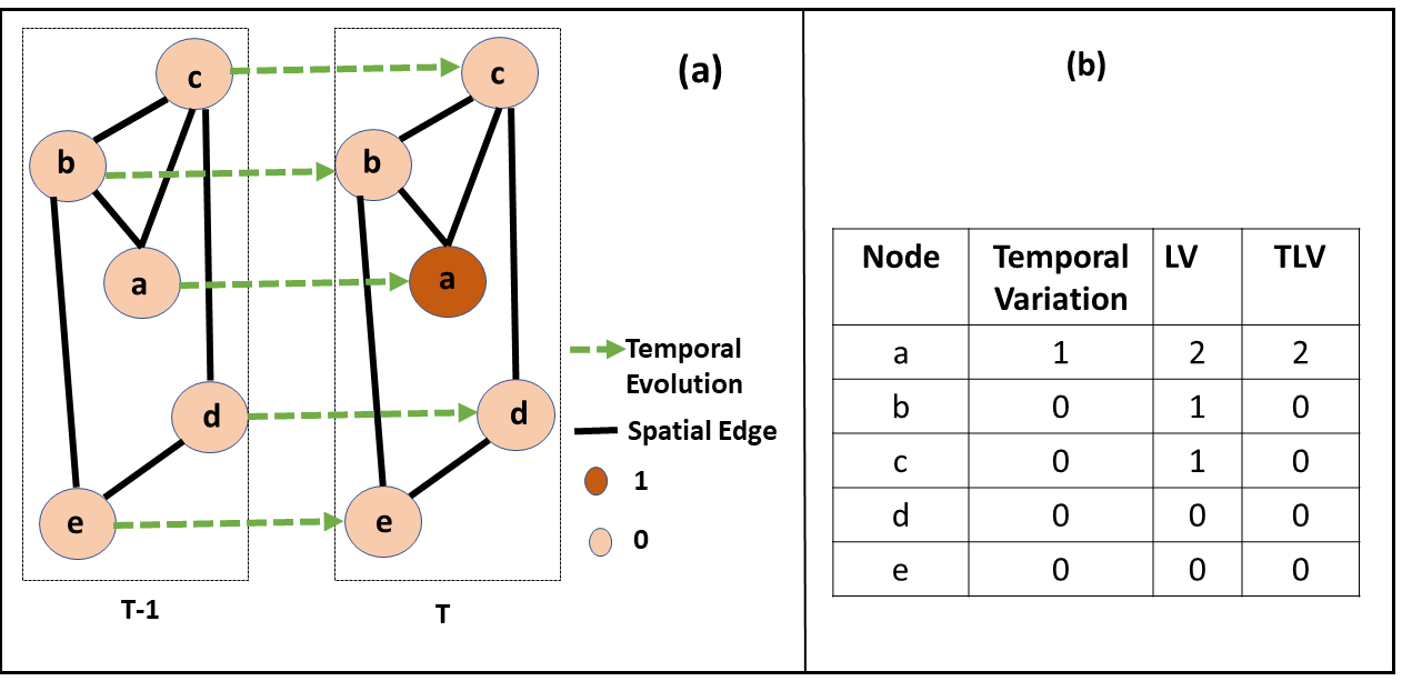
Fig. 1: Illustration of LV and TLV using a simple graph

A demonstration of LV and TLV is shown in Fig 1 using a five node graph, $\mathcal{V}=[a,b,c,d,e]$. The evolving graph signal (color coded) is shown in Fig 1(a) at times $T-1$ and $T$. Dashed arrows indicate the evolution of the graph signal in time. The temporal variation (3), local variation (2) and temporal local variation (3) are computed at time $T$ and shown in the table in Fig 1(b). The nodes $a,b$ and $c$ have non-zero $\mathcal{LV}$ reflecting the signal structure in the local neighbourhood. Since nodes $b$ and $c$ do not show temporal variation, their TLV is zero. Only node $a$ shows simultaneous variation in time and in its local neighbourhood giving it a non-zero TLV.

3 Epidemic analysis using GSP

3.1 Network SIR model

For illustration, we consider the standard SIR (susceptible-infected-recovered) model to depict how an epidemic propagates through a population. In SIR dynamics [4], a set of 3-coupled equations describe how the disease spreads within a location:

$$\dot{S}(t) = \displaystyle-\beta\frac{S(t)I(t)}{H},$$ (4)

$$\dot{I}(t) = \displaystyle\beta\frac{S(t)I(t)}{H}-\gamma I(t),$$ (5)

$$\dot{R}(t) = \gamma I(t),$$ (6)

where susceptible ($S$), infected ($I$), and recovered ($R$) are the three “compartments” of the population. The rates of disease transmission and average recovery are $\beta$ and $\gamma$, respectively. $H$ is the population size of that location. We now consider a spatial network of $N$ locations and employ a coupled population (meta-population) network with SIR dynamics. Let the $i^{th}$ location contain $H_{i}(i=1,2,...,N)$ individuals. We formulate the meta-population network equations [5, 17] by taking into account the dispersion through diffusion of normalized susceptible ($\mathcal{S}_{i}=\frac{S_{i}}{H_{i}}$), infected ($\mathcal{I}_{i}=\frac{I_{i}}{H_{i}}$), and recovered ($\mathcal{R}_{i}=\frac{R_{i}}{H_{i}}$) individuals,

$$\begin{array}[]{llll}\dot{\mathcal{S}_{i}}&=&\displaystyle-\beta_{i}\mathcal{S}_{i}\mathcal{I}_{i}+\frac{\kappa}{d_{i}}\sum_{j\in\mathcal{N}_{i}}W_{ij}(\mathcal{S}_{j}-\mathcal{S}_{i}),\\ \dot{\mathcal{I}_{i}}&=&\displaystyle\beta_{i}\mathcal{S}_{i}\mathcal{I}_{i}-\displaystyle\gamma_{i}\mathcal{I}_{i}+\frac{\kappa}{d_{i}}\sum_{j\in\mathcal{N}_{i}}W_{ij}(\mathcal{I}_{j}-\mathcal{I}_{i}).\end{array}$$ (9)

Here $W$ is the weighted adjacency matrix representing the spatial network and $d_{i}=\sum_{j\in\mathcal{N}_{i}}W_{ij}$ is the degree of the $i^{\rm th}$ node. The population migration is modeled through the diffusive term $\sum_{j\in\mathcal{N}_{i}}W_{ij}(X_{j}-X_{i})$ connected through two compartments ${X:\mathcal{S}_{i},\mathcal{I}_{i}}$. Strength of the migration is determined by $\kappa$. To solve the ODE equations, we utilised Runge-Kutta (RK4)[18] method with adaptive step size.

3.2 Methodology for identifying influential nodes

Given a graph $\mathcal{G}$ and the graph signal $X$, we wish to identify the nodes which significantly influence evolution of graph signal in time. We use the proposed graph variation metrics to develop an algorithm to detect these time-varying influential nodes. When applied to epidemic models, these influential nodes can help us understand the evolution of disease. Though we focus on epidemics, the method can potentially be applied to other time varying graph signals.

Let $\mathbf{x}_{t}(i)$ be the infected fraction of the population at node $i$ and time $t$. A temporal sliding window of length $\ell$ can be applied on $X$ to obtain a time-averaged graph signal $\mathcal{Y}$ if desired. An effective node classification method should capture the changes in the graph signal at both spatial and temporal scales. We classify the nodes by computing the graph variations on $\mathcal{Y}$ . The pseudo-code of our method is given in Algorithm 1 which takes as inputs the graph signal $X$ and the graph $\mathcal{G}=(\mathcal{V},\mathcal{E},W)$.

We first compute the graph variation (LV or TLV) of the input signal (line 4) to obtain $\mathcal{Y_{V}}$. This step can be replaced with high pass filter (for HPF analysis), $H_{\text{HPF}}$. Then, temporal mean is computed and a threshold $\tau$ is obtained from the mean of top $k\%$ of the nodes. Finally, the nodes are classified at each time step by comparing the graph variation with $\tau$ (lines $10-16$). For raw data ($\mathcal{Y}$) processing, we use lines $7-16$.

Algorithm 1 Identifying influential nodes
Input: $X$, $W$, $\kappa$

1:$\mathcal{Y}=$ time-windowed average of $X$

2:for $t=1,2,\ldots,T$ do

3:     for $i=1,2,\ldots,N$ do

4:         Compute $\mathcal{Y}_{V}(i,t)$ using (2) or (3)

5:     end for

6:end for

7:Compute average across time: $\mathbf{\mathcal{Y}_{VA}}=mean(\mathcal{Y}_{V})$

8:Sort in descending order: $\mathbf{\mathcal{Y}_{VA_{S}orted}}=sort(\mathbf{\mathcal{Y}_{VA}})$

9:Threshold: $\tau=$ mean of top $k\%$ of $\mathbf{\mathcal{Y}_{VA_{S}orted}}$

10:for $t=1,2,\ldots,T$ do

11:     for $i=1,2,\ldots,N$ do

12:         if  $\mathcal{Y}_{V}(i,t)\geq\tau$ then

13:              $j$ is a influential node

14:         end if

15:     end for

16:end for

4 Simulations and results

4.1 Graph construction

A random, distance-based graph is constructed. Uniform random sampling is performed within a $10\times 10$ square region to obtain $N=600$ graph nodes. Nearby nodes within a distance of $\alpha=1.667$ are connected with edge weight

$$W_{ij}=\begin{cases}e^{\frac{-{\text{dist}(i,j)}^{2}}{\tau^{2}}},\;\text{dist}(i,j)\leq\alpha,i\neq j\\ 0,&i=j.\end{cases}$$ (10)

where $\text{dist}(i,j)$ is the Euclidean distance between nodes $i$ and $j$ and parameter $\tau^{2}$ is the scaling factor. The generated graph tends to have both locally sparse and locally dense connections (shown in [19]). The intuition for considering distance-based graphs is that, in real-world scenarios, if roads play a major role in commute flow between locations, then infectious disease could propagate rapidly from an infected location to its nearest neighboring locations.

4.2 Epidemic data generation

We consider two scenarios for the creation of synthetic graph signal data $X$ from the network model:
Single perturbation: We chose a single node at random (node $\#588$) and introduced an initial infection ($0.2\%$ of the total population) while keeping the transmission rate ($\beta_{i}=\beta=0.3$) and recovery ($\gamma_{i}=\gamma=0.1$) rate same for all the network nodes. The initial $(t=0)$ infection is zero for all nodes except for node $\#588$. We use two coupling strengths – low ($\kappa=0.0001$) and high ($\kappa=0.1$), to simulate the epidemic data. Fig 2(a) shows time evolution of the initially infected node’s infection (we simulate $300$ time steps).

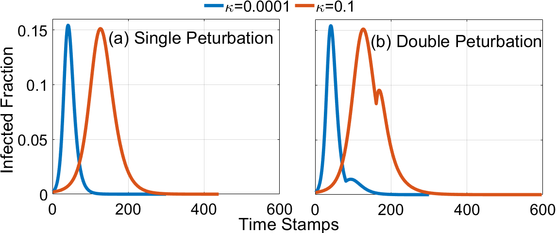
Fig. 2: Single and double perturbation at infected node $588$

Double perturbation: The process is the same as above, expect that when node $\#588$ reaches its peak value, a second perturbation is applied to it by altering the value of $\beta$ for a period of time. Specifically, the $\beta$ value is changed from $0.3$ to $0.8$, at $t=161$ when $\kappa=0.1$ ($t=81$ when $\kappa=0.0001$), for a period of $50$ time step. Fig 2(b) displays the temporal dynamics of infection for this node ($600$ time steps).
Data processing and plotting: Using the graph $G$ and graph signal $X$, we can carry out epidemic analysis using Algorithm 1 with results are presented in Fig 3. Various stages of epidemic are presented with arrow indicating the infected source node. The identified influential nodes are highlighted in red for visualization. We normalize data to $[0,1]$ and plot using the logarithmic scale.

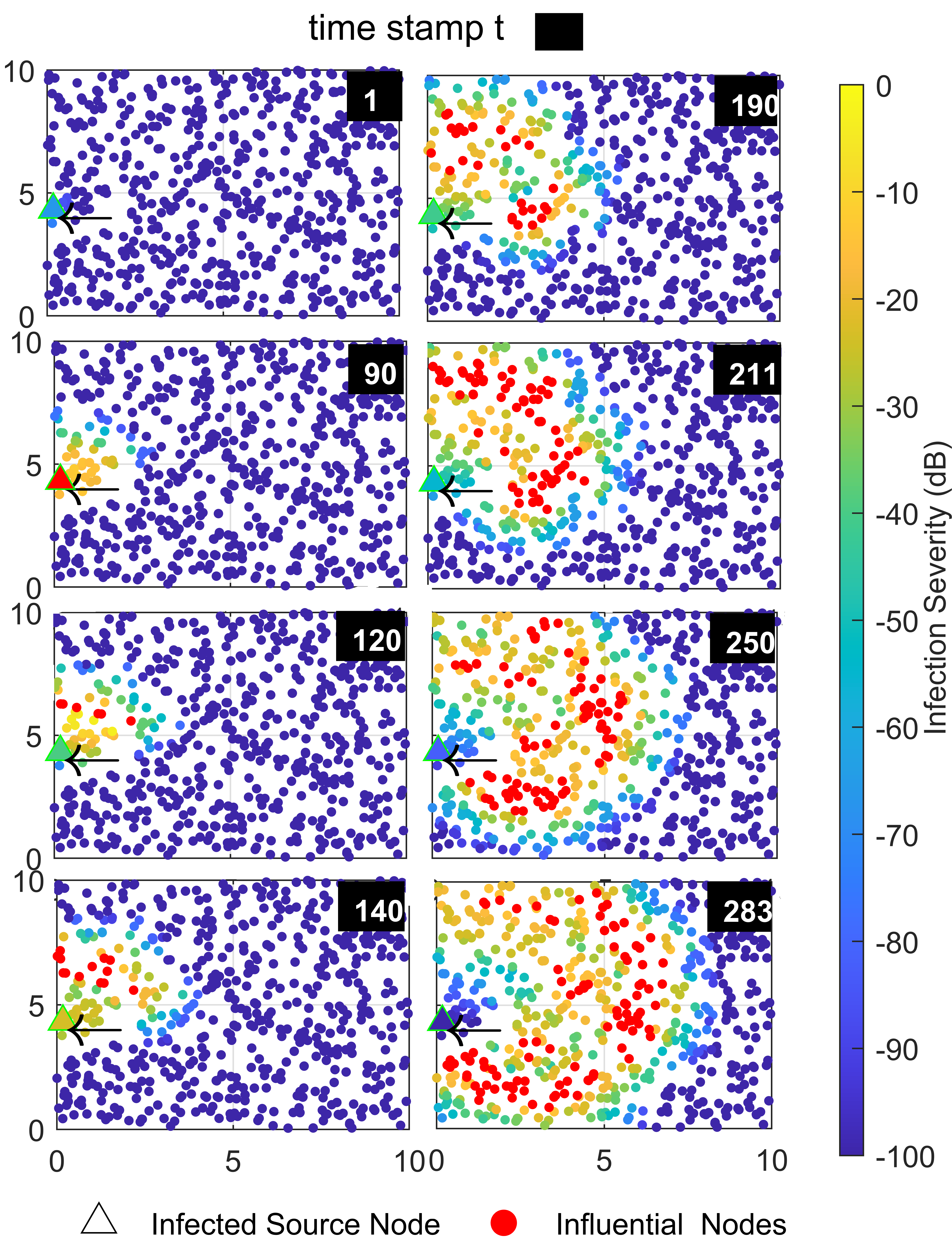
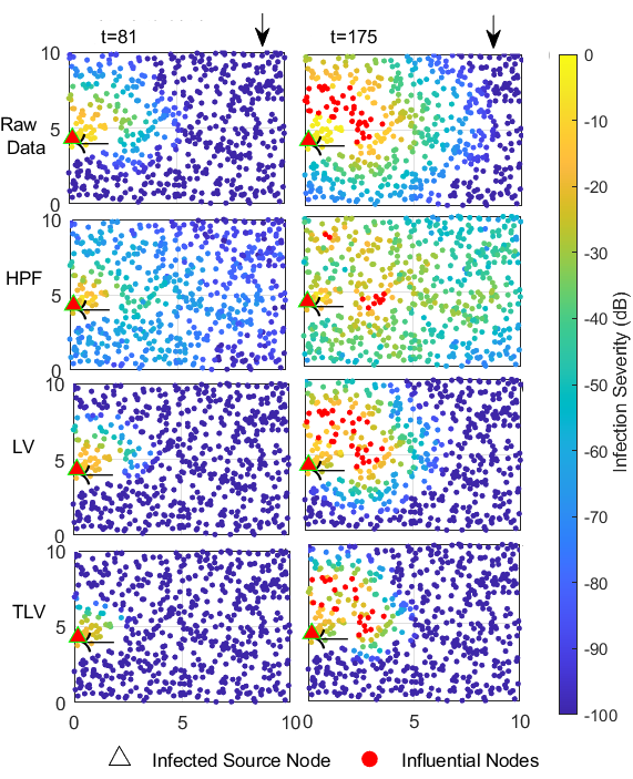
Fig. 3: Left: Evolution of disease from infected source node of single perturbation for $\kappa=0.1$ using TLV. Right: Identification of single and double perturbation at infected node $\#588$ for $\kappa=0.1$

4.3 Single perturbation analysis

Our primary objective here is to understand how disease spreads from a single infected node to the entire network. Results of Algorithm 1 when using temporal local variation are shown in Fig 3 (Left) at various time steps. The TLV detects the infected source node and shows how the epidemic spreads from the infected source node over the network. It can capture a variety of graph signal variations as indicated by differently colored nodes. Disease spread is driven by the influential spreader nodes highlighted in red. Identifying such nodes can help policy makers and health department to take precautionary measures in these regions.

4.4 Double perturbation analysis

Fig 3 (Right) shows the results of raw data, HPF, LV, and TLV on data from double perturbation simulation with $\kappa=0.1$. The methods are able to identify the infection source node $\#588$ during both the perturbations ($t=81$ and $t=175$). The HPF based processing does not capture the localized spreading of infection. This is because high frequency are not necessarily localized and show variation over the entire graph. As a result, it is unable to identify influential nodes. Additionally, it is unclear how many frequencies should be used for processing. Detailed plotting results of single and double perturbations for $\kappa=0.1$ and $0.0001$ are shown in [19].

Nodes with spatially varying graph signals are identified by LV, while nodes with spatio-temporally varying graph signals are identified by TLV. A majority of influential nodes detected by LV and TLV are same. Since TLV also accounts for temporal signal evolution, some of the detected nodes are different for LV and TLV. Though raw data captures nodes with highest infection, it is unable to capture infection activity (see [19] for details). The computational complexity of Algorithm 1 for LV and TLV is $\mathcal{O}(N^{2}T)$ whereas for HPF is $\mathcal{O}(N^{3}+N^{2}T))$ due to the eigenvalue decomposition.

5 Conclusion and future work

We examined the spreading pattern of disease from an infected source node using graph signal variation. We introduced low-complexity local variation metrics and devised an algorithm to identify influential nodes based on these metrics. Visualization of local variation and temporal local variation reveal major hot-spots which enable rapid spread of the disease. This can assist policymakers in identifying and classifying regions based on infection severity and follow up with necessary preventive actions. Our further study will focus on analyzing more complicated infection spread simulations and applying our algorithm on real-world data sets of disease.

References

- [1] V. Colizza, A. Barrat, M. Barthélemy, and A. Vespignani, “Predictability and epidemic pathways in global outbreaks of infectious diseases: the sars case study,” BMC medicine, vol. 5, no. 1, pp. 1–13, 2007.
- [2] A. Arenas, W. Cota, J. Gómez-Gardeñes, S. Gómez, C. Granell, J. T. Matamalas, D. Soriano-Paños, and B. Steinegger, “Modeling the spatiotemporal epidemic spreading of covid-19 and the impact of mobility and social distancing interventions,” Physical Review X, vol. 10, no. 4, pp. 041055, 2020.
- [3] M. UG. Kraemer, C. Yang, B. Gutierrez, C. Wu, B. Klein, D. M. Pigott, Open COVID-19 Data Working Group†, L. Du Plessis, N. R. Faria, R. Li, et al., “The effect of human mobility and control measures on the covid-19 epidemic in china,” Science, vol. 368, no. 6490, pp. 493–497, 2020.
- [4] MJ. Keeling and P. Rohani, “Modeling infectious diseases in humans and animals princeton univ,” Princeton, NJ, 2008.
- [5] D. Brockmann and D. Helbing, “The hidden geometry of complex, network-driven contagion phenomena,” science, vol. 342, no. 6164, pp. 1337–1342, 2013.
- [6] C. Hens, U. Harush, S. Haber, R. Cohen, and B. Barzel, “Spatiotemporal signal propagation in complex networks,” Nature Physics, vol. 15, no. 4, pp. 403–412, 2019.
- [7] V. Belik, T. Geisel, and D. Brockmann, “Natural human mobility patterns and spatial spread of infectious diseases,” Physical Review X, vol. 1, no. 1, pp. 011001, 2011.
- [8] A. Ortega, P. Frossard, J. Kovačević, J.MF. Moura, and P. Vandergheynst, “Graph signal processing: Overview, challenges, and applications,” Proceedings of the IEEE, vol. 106, no. 5, pp. 808–828, 2018.
- [9] D. I. Shuman, S. K. Narang, P. Frossard, A. Ortega, and P. Vandergheynst, “The emerging field of signal processing on graphs: Extending high-dimensional data analysis to networks and other irregular domains,” IEEE signal processing magazine, vol. 30, no. 3, pp. 83–98, 2013.
- [10] A. Sandryhaila and J. Moura, “Discrete signal processing on graphs: Graph fourier transform,” in 2013 IEEE International Conference on Acoustics, Speech and Signal Processing. IEEE, 2013, pp. 6167–6170.
- [11] A. Sandryhaila and J. MF. Moura, “Discrete signal processing on graphs: Frequency analysis,” IEEE Transactions on Signal Processing, vol. 62, no. 12, pp. 3042–3054, 2014.
- [12] A. Sandryhaila and J. Moura, “Discrete signal processing on graphs: Graph filters,” in 2013 IEEE International Conference on Acoustics, Speech and Signal Processing. IEEE, 2013, pp. 6163–6166.
- [13] Y. Li and G. Mateos, “Graph frequency analysis of covid-19 incidence to identify county-level contagion patterns in the united states,” in ICASSP 2021-2021 IEEE International Conference on Acoustics, Speech and Signal Processing (ICASSP). IEEE, 2021, pp. 3230–3234.
- [14] R. Pena, X. Bresson, and P. Vandergheynst, “Source localization on graphs via l1 recovery and spectral graph theory,” in 2016 IEEE 12th Image, Video, and Multidimensional Signal Processing Workshop (IVMSP). Ieee, 2016, pp. 1–5.
- [15] R. Geng, Y. Gao, H. Zhang, and J. Zu, “Analysis of the spatio-temporal dynamics of covid-19 in massachusetts via spectral graph wavelet theory,” IEEE Transactions on Signal and Information Processing over Networks, vol. 8, pp. 670–683, 2022.
- [16] S. Hosseinalipour, J. Wang, H. Dai, and W. Wang, “Detection of infections using graph signal processing in heterogeneous networks,” in GLOBECOM 2017-2017 IEEE Global Communications Conference. IEEE, 2017, pp. 1–6.
- [17] S. Ghosh, A. Senapati, J. Chattopadhyay, C. Hens, and D. Ghosh, “Optimal test-kit-based intervention strategy of epidemic spreading in heterogeneous complex networks,” Chaos: An Interdisciplinary Journal of Nonlinear Science, vol. 31, no. 7, pp. 071101, 2021.
- [18] C. Runge, “Über die numerische auflösung von differentialgleichungen,” Mathematische Annalen, vol. 46, no. 2, pp. 167–178, 1895.
- [19] S. Darapu, S. Ghosh, A. Senapti, C. Hens, and S. Nannuru, “Supplementarydocument,” https://github.com/DSudeepiniReddy/Icassp2023, 2022.