Transformer variational wave functions for frustrated quantum spin systems

Abstract

The Transformer architecture has become the state-of-art model for natural language processing tasks and, more recently, also for computer vision tasks, thus defining the Vision Transformer (ViT) architecture. The key feature is the ability to describe long-range correlations among the elements of the input sequences, through the so-called self-attention mechanism. Here, we propose an adaptation of the ViT architecture with complex parameters to define a new class of variational neural-network states for quantum many-body systems, the ViT wave function. We apply this idea to the one-dimensional $J_{1}$-$J_{2}$ Heisenberg model, demonstrating that a relatively simple parametrization gets excellent results for both gapped and gapless phases. In this case, excellent accuracies are obtained by a relatively shallow architecture, with a single layer of self-attention, thus largely simplifying the original architecture. Still, the optimization of a deeper structure is possible and can be used for more challenging models, most notably highly-frustrated systems in two dimensions. The success of the ViT wave function relies on mixing both local and global operations, thus enabling the study of large systems with high accuracy.

Introduction. Variational approaches for studying quantum many-body systems have proved fundamental for understanding the properties of extremely complicated physical systems, famous examples being the Bardeen-Cooper-Schrieffer state Bardeen et al. (1957) and Laughlin Laughlin (1983) wave functions to explain superconductivity and fractional quantum Hall effect, respectively. Given the exponential growth of the many-body Hilbert space, a compact representation of the ground state, encoding the correct physical properties, is a highly non-trivial task for strongly-interacting systems. Recently, a class of wave functions, based on neural networks, has been introduced and developed Carleo and Troyer (2017); Glasser et al. (2018). Starting from Restricted Boltzmann Machines (RBMs) Carleo and Troyer (2017), which are the simplest neural-network Ansatz (namely only one fully-connected hidden layer), numerous studies have been carried out testing different types of architectures; examples include Convolutional-Neural Networks (CNNs) Choo et al. (2019); Liang et al. (2018); Chen et al. (2022); Roth and MacDonald (2021), Recurrent-Neural Networks (RNNs) Hibat-Allah et al. (2020, 2022), Autoregressive-Neural Networks Luo et al. (2021); Sharir et al. (2020), but also combinations of neural networks with standard variational wave functions (e.g., Gutzwiller-projected fermionic ones) Nomura et al. (2017); Ferrari et al. (2019).

In the last few years, the Transformer architecture Vaswani et al. (2017) has become the state-of-art choice in natural-language processing tasks. Its key feature is the ability to model relationships among all elements of an input sequence (regardless of their positions), by efficiently transforming input sequences into abstract representations. Inspired by successes in natural-language processing, very small modifications led to the so-called Vision Transformer (ViT) Dosovitskiy et al. (2021), which has been applied to image classification tasks, achieving competitive results with respect to state-of-art deep CNNs, while being much more efficient than them. Within many-body problems, Transformer networks have recently been employed in the context of lattice gauge theories Luo et al. (2021), to perform quantum tomography in presence of noise Cha et al. (2021), and for real- and imaginary-time evolutions of quantum systems Luo et al. (2022).

In this Letter, we demonstrate that the ViT architecture can be adapted to define a new class of neural-network quantum states, here dubbed as ViT wave functions. We apply our Ansatz to the one-dimensional $J_{1}$-$J_{2}$ Heisenberg model, whose Hamiltonian is defined by

$$\hat{H}=J_{1}\sum_{R}\hat{\bm{S}}_{R}\cdot\hat{\bm{S}}_{R+1}+J_{2}\sum_{R}\hat{\bm{S}}_{R}\cdot\hat{\bm{S}}_{R+2}\,$$ (1)

where $\hat{\bm{S}}_{R}=(S_{R}^{x},S_{R}^{y},S_{R}^{z})$ is the $S=1/2$ spin operator at site $R$ and $J_{1}>0$ and $J_{2}\geq 0$ are nearest- and next-nearest-neighbor antiferromagnetic couplings, respectively. Its phase diagram is well established by analytical and numerical studies White and Affleck (1996). For small values of $J_{2}/J_{1}$, the ground state has power-law spin-spin correlations and the excitation spectrum is gapless; for large values of $J_{2}/J_{1}$, the ground state is two-fold degenerate, leading to long-range dimer order (but exponentially decaying spin-spin correlations), and the spectrum is fully gapped. These two phases are separated by a critical point at $(J_{2}/J_{1})_{c}=0.241167\pm 0.000005$ Eggert (1996); Sandvik (2010). Interestingly, for $J_{2}/J_{1}>0.5$, incommensurate (but short-range) spin-spin correlations have been found, whereas dimer–dimer correlations are always commensurate. In the following, we assess the ground-state properties of the $J_{1}$-$J_{2}$ model on finite clusters, imposing periodic boundary conditions.

From the numerical perspective, density-matrix renormalization group (DMRG) White (1992) or its modern variations based upon tensor networks Ansätze Schollwöck (2011) represent one of the few approaches that can accurately assess the ground-state properties of frustrated systems in one dimension, as the $J_{1}$-$J_{2}$ model of Eq. (1). In fact, the main limitation to the use of quantum Monte Carlo techniques Becca and Sorella (2017) relies on the unknown sign structure of the ground-state wave function, which prevents one to perform unbiased projection techniques (except for $J_{2}=0$, where the so-called Marshall sign rule applies Marshall (1955)). The non-trivial sign structure represents also an obstacle to the definition of accurate variational wave functions. For example, Gutzwiller-projected fermionic states Ferrari et al. (2018) have a limited power to reproduce the correct signs of the ground state for $J_{2}/J_{1}>0.5$ Viteritti et al. (2022). By contrast, RBM states are able to reach an excellent accuracy; however, they suffer from poor scaling behavior, due to their fully-connected structure in which a single hidden layer is connected to all physical degrees of freedom Viteritti et al. (2022). This fact limits the applicability of RBMs to relatively small clusters. In this respect, CNN wave functions have been introduced to deal with local structures and deep architectures are necessary to build long-range correlations, thus introducing severe problems in the optimization procedure (e.g., diverging or vanishing gradients). RNNs Ansätze have been also considered, which recurrently process inputs of a sequence one by one, implying that they cannot be parallelized; in addition, since not all elements of the network are directly connected, long-range correlations are built from short-range ones, thus making the learning process not straightforward Bengio et al. (1994).

In order to overcome these problems, we propose a simplified version of the standard ViT architecture. The main advantage of this Ansatz lies in the possibility to mix both local and global structures, thus limiting the number of variational parameters and simplifying the learning process (see below). We emphasize that a complex parametrization is adopted without an a priori encoding of the sign structure (i.e., no information about the exact signs). In this work, we show that the ViT wave function can reach very high accurate results compared to DMRG calculations, even on large clusters, with less then one thousand parameters and few computational resources compared to other neural-network wave functions. Most importantly, the ViT accuracy can be systematically improved by changing the hyper-parameters of the architecture.

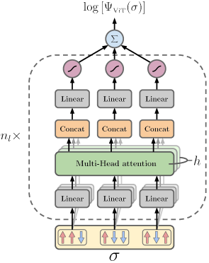
Figure 1: Scheme of the ViT wave function. The input spin configuration $\sigma$ is split into patches of size $b$ (which define a set of $N$ vectors of dimension $b$). Each of them is linearly projected $h$ times with different linear projections to produce $N$ vectors of dimensions $r=d/h$. Then the attention function is applied in parallel and the $h$ different $r$ dimensional output vectors $\bm{A}_{i}^{\mu}$ are obtained. Then, they are concatenated to a $d$ dimensional vector $\text{Concat}(\bm{A}_{i}^{1},\dots,\bm{A}_{i}^{h})$ and, after another linear projection, the non-linear function log[cosh($\cdot$)] is applied. This architecture can be replicated and stacked $n_{l}$ times. The last layer simply sums all the outputs and returns the logarithm of the ViT wave function.

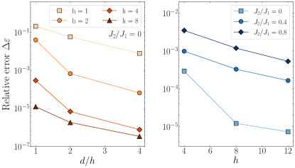
Figure 2: Relative error $\Delta\varepsilon=|(\text{E}_{\rm ViT}-\text{E}_{\rm DMRG})/\text{E}_{\rm DMRG}|$ of the ViT wave function by varying the hyper-parameters of the architecture for a cluster with $L=100$ sites. Left panel: $\Delta\varepsilon$ as a function of $d/h$, with a fixed number of heads $h$, for the unfrustrated case. Right panel: $\Delta\varepsilon$ as a function of the number of heads $h$, with $d/h=1$, for different values of frustration ratio. The reference energies are computed by DMRG Pippan et al. (2010) with a bond dimension up to $\chi=600$ obtaining $E/J_{1}=-0.4432295$ for $J_{2}/J_{1}=0$, $E/J_{1}=-0.3803882$ for $J_{2}/J_{1}=0.4$, and $E/J_{1}=-0.4216664$ for $J_{2}/J_{1}=0.8$.

Methods. The fundamental ingredient of a Transformer is the self-attention mechanism. Given a sequence of $N$ input vectors $(\bm{x}_{1},\dots,\bm{x}_{N})$, for each of them three new vectors are computed, $\bm{q}_{i}=\text{Q}\bm{x}_{i}$, $\bm{k}_{i}=\text{K}\bm{x}_{i}$, and $\bm{v}_{i}=\text{V}\bm{x}_{i}$, where Q, K, V are generic rectangular matrices of parameters. The attention vectors are then constructed, $\bm{A}_{i}=\sum_{j=1}^{N}\alpha(\bm{q}_{i},\bm{k}_{j})\bm{v}_{j}$, where the attention weights $\alpha(\bm{q}_{i},\bm{k}_{j})$ determine how much the $j$-th input vector should contribute to $\bm{A}_{i}$, which is the subsequent representation of the $i$-th input. The functional form of these weights can be chosen according to the task Tay et al. (2020). To improve the performance of the model, multi-head attention can be considered, where a set of matrices $Q^{\mu}$, $K^{\mu}$, and $V^{\mu}$, with $\mu=1,\dots,h$ (with $h$ the number of heads) is defined, thus leading to a set of attention vectors $\bm{A}^{\mu}_{i}$. The latter ones are computed in parallel, concatenated together, and linearly combined. Finally, each output vector of the multi-head attention is fed separately and identically to a non linearity. In general, this whole architecture is replicated $n_{l}$ times.

Our goal is to use the Transformer to parameterize the many-body wave function, in order to map spin configurations of the Hilbert space $\sigma=(\sigma_{1},\dots,\sigma_{L})$, with $\sigma_{R}=2S_{R}^{z}=\pm 1$, to complex numbers $\Psi(\sigma)$. We take inspiration from the ViT Dosovitskiy et al. (2021) introduced for computer vision tasks, where the images are split into patches and these are taken as the input sequence to a Transformer. In the same way, starting from a spin configuration $\sigma=(\sigma_{1},\dots,\sigma_{L})$, we split it into $N$ patches of $b$ elements: $\bm{x}_{i}=(\sigma_{(i-1)b+1},\dots,\sigma_{(i-1)b+b})$, for $i=1,\dots,N$ (the total number of sites must be a multiple of $b$). The sequence of these patches is then used to compute the attention vectors. Then, a simplification of the original ViT is considered, taking the attention weights only depending on positions $i$ and $j$, but not on the actual values of the spins in these patches, thus leading to:

$$\bm{A}^{\mu}_{i}=\sum_{j=1}^{N}\alpha^{\mu}_{ij}\text{V}^{\mu}\bm{x}_{j},$$ (2)

where $V^{\mu}$ is a $r\times b$ matrix with $r=d/h$, and $d$ is the so-called embedding dimension that must be a multiple of the number of heads $h$. This approach is dictated by the fact that the attention weights should mainly depend on the relative positions among groups of spins and not on the actual values of the spins in the patches. This is expected to be true when the patches are far apart and is extended for generic positions $i$ and $j$. Finally, after the concatenation of the heads, a further linear projection is taken, before the non linearity, here chosen as log[cosh($\cdot$)]. This block can be repeated $n_{l}$ times before applying the output layer in which all the values are summed to obtain the logarithm of the ViT wave function $\Psi_{\text{ViT}}(\sigma)$ (see Fig. 1).

In order to study frustrated quantum spin models with a non-positive ground state (in the computational basis), we choose all the parameters to be complex numbers. Furthermore, a translationally-invariant wave function with $k=0$ can be easily defined by considering the following two steps. First, we adapt the relative positional encoding Shaw et al. (2018) to periodic systems, taking $\alpha_{i,j}^{\mu}=\alpha_{i-j}^{\mu}$; as a result, the number of variational parameters for computing the attention vectors (2) is reduced from $O(L^{2})$ to $O(L)$. This procedure induces translational invariance between patches. To include also the one within patches, we perform the linear combination:

$$\tilde{\Psi}_{\text{ViT}}(\sigma)=\sum_{r=0}^{b-1}\Psi_{\text{ViT}}(\text{T}_{r}\sigma),$$ (3)

where $\text{T}_{r}$ is the translation operator. We emphasize that this approach requires a small summation (of $b$ terms), which does not grow with the system size $L$.

The optimization process of all the complex parameters is obtained by using standard variational Monte Carlo techniques, namely the so-called Stochastic Reconfiguration approach (see the Supplemental Material for more details). In the following, we mainly take $n_{l}=1$, which represents the simplest possible adaptation of the Transformer architecture; indeed, even within this drastic assumption, we obtain excellent results in both gapless and gapped phases. At the end, we show the effect of a deeper network with $n_{l}>1$. All the simulations are performed by fixing the patch size $b=4$.

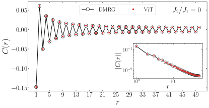
Figure 3: The isotropic spin-spin correlations in real space $C(r)$ as computed by the ViT wave function (full dots) for the unfrustrated Heisenberg model ($J_{2}/J_{1}=0$) on a cluster with $L=100$ sites. The DMRG results are also shown for comparison (empty circles). Inset: Log-log plot of the same correlation function.

Results. We start by discussing how the accuracy of the ViT wave function with one layer can be systematically improved by varying its two hyper-parameters, i.e., the number of heads $h$ and the ratio $r=d/h$. We consider a cluster with $L=100$ sites and three different values of the frustration ratio: $J_{2}/J_{1}=0$ (unfrustrated, gapless), $0.4$ (weakly-frustrated, gapped), and $0.8$ (strongly-frustrated, gapped); the reference energy is computed by using the standard DMRG approach (imposing periodic-boundary conditions on the Hamiltonian Pippan et al. (2010)). In Fig. 2, we show the accuracy of the ground-state energy for the unfrustrated case as a function of $d/h$ fixing the number of heads $h$, and for the three values of $J_{2}/J_{1}$ when increasing the number of heads $h$, at fixed ratio $d/h$. Even though there is a general difficulty in reconstructing the exact sign structure in highly-frustrated regimes Viteritti et al. (2022); Westerhout et al. (2020); Szabó and Castelnovo (2020); Park and Kastoryano (2021); Bukov et al. (2021), we obtain an excellent approximation of the correct energy for all the values of $J_{2}/J_{1}$ that have been considered, e.g., an accuracy $\Delta\varepsilon\lesssim 0.1\%$ for $J_{2}/J_{1}=0.8$ and $\Delta\varepsilon\approx 0.01\%$ for $J_{2}/J_{1}=0.4$.

Let us now move to the analysis of the correlation functions. From the previous results, we choose $h=8$ and $d/h=1$ as a good compromise between accuracy and complexity, for which the network can be trained on $L=100$ sites in a few hours on ten CPUs or in a few minutes on a GPU. The spin-spin correlations are defined as

$$C^{\nu\nu}(r)=\frac{1}{L}\sum_{R=0}^{L-1}\langle\hat{S}^{\nu}_{R}\hat{S}^{\nu}_{R+r}\rangle,$$ (4)

where $\nu=x$, $y$, or $z$ and $\langle\dots\rangle$ represents the expectation value over the variational quantum state. In particular, we focus on isotropic spin-spin correlations $C(r)=[C^{zz}(r)+C^{xx}(r)+C^{yy}(r)]/3$ and the corresponding structure factor in Fourier space $S(k)=\frac{1}{L}\sum_{r=0}^{L-1}\text{e}^{ikr}C(r)$. In Fig. 3, we show the results of the real-space correlations $C(r)$ for the unfrustrated Heisenberg model ($J_{2}/J_{1}=0$) on a cluster with $L=100$ sites, comparing them to the DMRG outcomes (with periodic-boundary conditions). Remarkably, the ViT Ansatz is able to match the DMRG calculations at all distances, demonstrating that the global structure of the multi-head attention layer is able to build the algebraic long-range tail.

The high flexibility of the ViT state is also demonstrated by considering the three different regimes, with commensurate (i.e., $S(k)$ peaked at $k=\pi$) or incommensurate (i.e., $S(k)$ peaked at $k\neq\pi$) correlations, see Fig. 4.

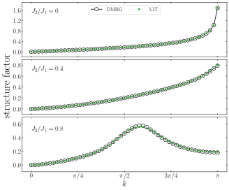
Figure 4: The spin-spin structure factor $S(k)$ as computed by the ViT wave function (full dots) for $J_{2}/J_{1}=0$ (upper panel), $J_{2}/J_{1}=0.4$ (middle panel) and $J_{2}/J_{1}=0.8$ (lower panel) on a cluster with $L=100$ sites. The DMRG results are also shown for comparison (empty circles).

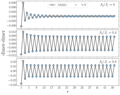
Figure 5: Dimer-dimer correlations as computed by the ViT wave function (full circles) for $J_{2}/J_{1}=0$ (upper panel), $J_{2}/J_{1}=0.4$ (middle panel) and $J_{2}/J_{1}=0.8$ (lower panel) on a cluster with $L=100$ sites. The DMRG results are also shown for comparison (empty circles).

The gapped phase is characterized by a finite dimer order (implied by the two-fold degeneracy of the ground state, in the thermodynamic limit). On any finite system, there is an exponentially small gap between the two states, with $k=0$ and $k=\pi$, and the insurgence can be detected from the connected dimer-dimer correlations:

$$D(r)=\frac{1}{L}\sum_{R=0}^{L-1}\langle\hat{S}^{z}_{R}\hat{S}^{z}_{R+1}\hat{S}^{z}_{R+r}\hat{S}^{z}_{R+r+1}\rangle-[C^{zz}(r=1)]^{2},$$ (5)

where $C^{zz}(r=1)$ is the $z$ component of the spin-spin correlation function at distance $r=1$ defined in eq. (4). Notice that this definition considers only the $z$ component of the spin operators Capriotti et al. (2003). In Fig. 5, we show the results for the three values of $J_{2}/J_{1}$ considered in this work. Again, the agreement with DMRG calculations is excellent in all cases, and the ViT state is able to perfectly reproduce the presence of dimer order.

DeepViT. The ViT wave function can be systematically improved by stacking multiple Transformer layers, i.e., $n_{l}>1$. The optimization of deep networks is difficult with standard protocols, then we develop a procedure based on the physical interpretation of the attention weights. We start by setting for each head and layer $\alpha_{i-j}=0$ if $|i-j|>{\rm cut}$, with ${\rm cut}<L/b$, training only the remaining weights. Small cut values (e.g., ${\rm cut}=1$) are good starting points for stable optimizations. Then the cut is relaxed until reaching $L/b$, where all-to-all connections among the inputs of each layer are restored. As an example, the results for the Heisenberg model with $L=40$ are shown in Fig. 6. Here, we take $n_{l}=4$ (each layer has $h=2$ and $d/h=2$) and perform the optimization stages with ${\rm cut}=1,\dots,10$. Every time, when the cut is relaxed, the accuracy of the energy improves. We stress that the optimization is performed without Marshall sign prior.

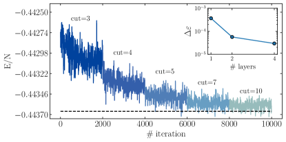
Figure 6: Optimization of the DeepViT with $n_{l}=4$, where each layer has $h=2$ and $d/h=2$, for the Heisenberg model with $L=40$ sites. Along the process, the cut in the attention is fixed and progressively increased from $1$ to $10$ (the first two values are not shown for better readability). At the end, once the cut has been completely relaxed, the full translational invariance is restored [see Eq. (3)] to compute the accuracy in the energy. Inset: Relative error $\Delta\varepsilon$ of the DeepViT wave function by varying the number of layers. The reference energy is computed by DMRG Pippan et al. (2010) with a bond dimension up to $\chi=600$ obtaining $E/J_{1}=-0.443663$.

Conclusions. We have introduced a promising class of variational wave functions, which are based upon Transformer neural-network architectures (in particular, Vision Transformers). Their main advantages, with respect to previously defined Ansätze, is the mixing of local and global structures, which makes them very flexible to describe a variety of different quantum phases, with both gapped and gapless spectra. Remarkably, even working with a relatively simple architecture, with $n_{l}=1$, excellent results are obtained for a frustrated spin model in one spatial dimension. Generalizations to one-dimensional models with long-range interactions (e.g., the Haldane-Shastry model Haldane (1988); Shastry (1988)) or two-dimensional models, where ground-state properties are still under debate, are desirable and represent the topic for future investigations, including the calculation of long-range entanglement properties Zhang et al. (2011). We expect that for these systems the depth of the network could be important to achieve competitive results with respect to state-of-art numerical methods.

Supplemental Material

Optimization of the variational wave function

The goal of the optimization procedure is the minimization of the variational energy

$$E(\mathcal{W})=\langle\hat{H}\rangle_{\mathcal{W}}=\frac{\langle{\Psi_{\mathcal{W}}}|\hat{H}|{\Psi_{\mathcal{W}}}\rangle}{\langle{\Psi_{\mathcal{W}}}|{\Psi_{\mathcal{W}}}\rangle}\ ,$$ (6)

with respect to the variational parameters $\{\mathcal{W}\}$. To perform the optimization we employ the Stochastic Reconfiguration method Sorella (2005) which we briefly describe in the following (for a detailed description see reference Becca and Sorella (2017)).
For each parameter $w_{\alpha}\in\{\mathcal{W}\}$ we define the corresponding operator $\hat{\mathcal{O}}_{\alpha}$, diagonal in the computational basis $\langle\sigma|\hat{\mathcal{O}}_{\alpha}|\sigma^{\prime}\rangle={\mathcal{O}}_{\alpha}(\sigma)\delta_{\sigma,\sigma^{\prime}}$, whose matrix elements are

$${\mathcal{O}}_{\alpha}=\frac{\partial\log\left(\Psi_{\mathcal{W}}(\sigma)\right)}{\partial w_{\alpha}}\ .$$ (7)

At each optimization step the variational parameters are updated according to

$$w_{\alpha}^{\prime}=w_{\alpha}+\eta\sum_{\beta}S_{\alpha,\beta}^{-1}f_{\beta}\ ,$$ (8)

where $\eta$ is the learning rate, an hyperparameter of the optimization process, $f_{\beta}$ are the forces

$$f_{\beta}=-\frac{\partial\langle\hat{H}\rangle_{\mathcal{W}}}{\partial w_{\beta}}=-2\Re\{\langle\hat{H}^{*}\hat{O}_{\beta}\rangle_{\mathcal{W}}-\langle\hat{H}^{*}\rangle_{\mathcal{W}}\langle\hat{O}_{\beta}\rangle_{\mathcal{W}}\}\ ,$$ (9)

and $S^{-1}$ is the inverse of the covariance matrix

$$S_{\alpha,\beta}=\Re\{\langle\hat{O}^{\dagger}_{\alpha}\hat{O}_{\beta}\rangle_{\mathcal{W}}-\langle\hat{O}_{\alpha}^{\dagger}\rangle_{\mathcal{W}}\langle\hat{O}_{\beta}\rangle_{\mathcal{W}}\}\ .$$ (10)

The expectation values $\langle\cdot\cdot\cdot\rangle_{\mathcal{W}}$, defined with respect to the probability distribution $|\Psi_{\mathcal{W}}(\sigma)|^{2}$, are estimated stochastically using the Metropolis algorithm with a sample size of $O(10^{3}\div 10^{4})$. In addition, given the SU(2) spin symmetry of the $J_{1}$-$J_{2}$ Heisenberg model, the sampling procedure for the study of the ground state properties can be limited to the $S^{z}=\sum_{R}S^{z}_{R}=0$ sector, thereby in order to conserve the total magnetization, nearest- and next-nearest neighbor spin exchanges are considered. The convergence of the optimization process, for a chain of $L=100$ sites considered in this work, is achieved in $O(10^{2}\div 10^{3})$ steps setting the learning rate $\eta$ to $10^{-2}\div 10^{-3}$. We point out that the $S$-matrix defined in Eq. (10) can be not invertible due to a redundant parametrization of the variational state, which usually happens when the wave function has a large number of parameters. In order to prevent numerical instabilities in the inversion of the matrix, we regularize it by shifting the diagonal elements of the $S$-matrix by a small perturbation $S_{\alpha,\alpha}\rightarrow S_{\alpha,\alpha}+\varepsilon$, typical values are $\varepsilon\sim 10^{-3}\div 10^{-4}$.