Safe and Adaptive Decision-Making for Optimization of Safety-Critical Systems: The ARTEO Algorithm
Abstract
We consider the problem of decision-making under uncertainty in an environment with safety constraints. Many business and industrial applications rely on real-time optimization to improve key performance indicators. In the case of unknown characteristics, real-time optimization becomes challenging, particularly because of the satisfaction of safety constraints. We propose the ARTEO algorithm, where we cast multi-armed bandits as a mathematical programming problem subject to safety constraints and learn the unknown characteristics through exploration while optimizing the targets. We quantify the uncertainty in unknown characteristics by using Gaussian processes and incorporate it into the cost function as a contribution which drives exploration. We adaptively control the size of this contribution in accordance with the requirements of the environment. We guarantee the safety of our algorithm with a high probability through confidence bounds constructed under the regularity assumptions of Gaussian processes. We demonstrate the safety and efficiency of our approach with two case studies: optimization of electric motor current and real-time bidding problems. We further evaluate the performance of ARTEO compared to a safe variant of upper confidence bound based algorithms. ARTEO achieves less cumulative regret with accurate and safe decisions.
1 INTRODUCTION
In most sequential decision-making problems under uncertainty, there exists an unknown function with noisy feedback that the decision-maker algorithm needs to sequentially estimate and optimize to reveal the decisions leading to the highest reward. Each decision receives an instantaneous reward with an initially unknown distribution in a stochastic optimization setting. In this setting, initial decisions are made based on some heuristics, and incurred reward is memorized to exploit for the next decisions. Therefore, the uncertainty due to unknown characteristics decreases while new decisions are made based on previous reward observations. Even though more exploration can help to optimize the decisions by revealing more information in each iteration, it could be very expensive to evaluate the unknown function for many applications. Therefore, there is a need to balance exploring unknown decision points and exploiting previous experiences. The trade-off between exploration and exploitation is extensively studied in the literature, and the multi-armed bandit (MAB) approaches with confidence bounds are suggested to solve this problem by optimally balancing exploration and exploitation (Bubeck et al., 2012).
Related work. The idea of using confidence bounds to balance the exploration-exploitation trade-off through the optimism principle first appeared in the work of Lai and Robbins (1985) with the utilization of the upper confidence bound (UCB). Since then, it led to the development of UCB algorithms for stochastic bandits with many arms (Lattimore and Szepesvári, 2020). Many efficient algorithms build for bandit problems having a cost or reward function under certain regularity conditions (Dani et al., 2008; Bubeck et al., 2009). In Srinivas et al. (2010), the authors divided the stochastic optimization problem into two objectives: (1) unknown function estimation from noisy observations and (2) optimization of the estimated function over the decision set. They used kernel methods and Gaussian processes (GPs) to model the reward function since these methods encode the regularity assumptions through kernels (Rasmussen, 2004). Even though these methods are very successful to model and optimize unknown reward functions, they do not consider safety constraints.
In safety-critical systems, it is not possible to do exploration in some parts of the decision space due to safety concerns, which are modelled as safety constraints in optimization. Many industrial applications fall under the safety-critical systems due to their risk of danger to human life, leading to substantial economic loss, or causing severe environmental damage. For example, we can consider a chemical process plant as a safety-critical operation since we need to satisfy the constraints of chemical reactions and surrounding processes to not cause a hazardous event for the environment and human operators. Therefore, if we want to approximate the unknown characteristics and optimize a process in this plant, we need to utilize safe exploration algorithms which allow only the exploration of feasible decision points by enforcing safety constraints. In this work, we define a feasible decision point in the given decision set as satisfying the safety and other constraints of the given problem.
The safe exploration problem has been studied by formalizing it as both bandit and Markov Decision Processes (MDPs) problems (Schreiter et al., 2015; Turchetta et al., 2016; Wachi et al., 2018; Turchetta et al., 2019). In Sui et al. (2015), the authors have introduced the SafeOpt algorithm and showed it is possible that safely optimize a function with an unknown functional form by creating and expanding a safe decision set through safe exploration under certain assumptions. They also provided the safety guarantee of SafeOpt by using the confidence bounds construction method of Srinivas et al. (2010). These safe exploration algorithms are applied to many control and reinforcement learning problems and proved their success in those domains (Berkenkamp et al., 2016; Kabzan et al., 2019). However, these algorithms either require an exploration phase or apply a trade-off strategy between optimal decisions and exploration. There are some real-world applications such as industrial processes which cannot afford an exclusive exploration phase or require following optimization goals of the system even in the explored points. For example, any deviation from target satisfaction in an industrial process may cause high costs to the plant or damage the reputation of the responsible party. Thus, there is a need to consider the exploration in an adaptive manner in accordance with the requirements of the environment and this aspect is not covered by existing safe exploration algorithms.
Our contributions. In this paper, we propose a novel safe Adaptive Real-Time Exploration and Optimization (ARTEO) algorithm, where we cast multi-armed bandits as a mathematical programming problem subject to safety constraints for the optimization of safety-critical systems. Our contribution is posing a further constraint to the safe exploration by instructing the algorithm to avoid decisions not satisfying the optimization goals of the safety application. This constraint discourages exploration which makes it harder to learn unknown rewards in the MAB setting. To compensate for that, we incorporate the exploration as a contribution to the cost function in an adaptive manner by encouraging explicitly to take decisions at points with high uncertainty which is quantified by the covariance of GP models. We adaptively control the size of this contribution in accordance with the requirements of the environment. ARTEO uses GPs to model how the unknown parameters of an application change based on external factors such as inputs and optimization goals, make new decisions when a change in the optimization goals or in the given input is occurred and explores new decision points with either a change in the optimization goals or based on uncertainty. We establish the safety of ARTEO by constructing the confidence bounds as Srinivas et al. (2010) and showing certain assumptions hold in our setting. We demonstrate the safety and efficiency of our algorithm using two real-world examples: the electric current optimization in electric motors and the high-dimensional online bid optimization problem. In the first experiment, the results show that we are able to successfully estimate and optimize the current without any constraint violation by applying ARTEO. In the second experiment, our approach satisfies the constraints while yielding more profitable outcomes.
2 PROBLEM STATEMENT AND BACKGROUND
We want to find a sequence of decisions, , so that a certain cost function is minimised. At each iteration , where , the cost function is dependent on the decision , and on the system characteristics . Here, and is the set of unknowns with elements, where is the index of an unknown, and , with being the number of decision variables. The characteristics are determined by the decision , i.e. where . After making a decision , we obtain a noisy measurement, , where and is an -sub-Gaussian noise with a fixed constant (Agrawal and Goyal, 2013). We assume that we know the functional form of , but the functional form of is unknown. Furthermore, at every iteration, the decision must satisfy the constraints , where with denoting the number of constraints. The value of is called a safety threshold. Thus, we can formalise our optimization problem at time as:
| (1) |
where are decision variables. If we know , we can solve the problem as an optimization problem with noise. For instance, we could use the concept of real-time optimization (RTO) from the process control domain (Naysmith and Douglas, 2008) and use the approach proposed by Petsagkourakis et al. (2021). However, the characteristics are unknown. Thus, at every iteration , we first solve an estimation problem to find , then solve the optimization problem (1). Solving an optimization problem by combining estimation then optimization is a common approach (Zhang et al., 2022; Fu and Levine, 2021). However, few approaches quantify the uncertainty inherent in the estimation of . In the current paper, we propose to estimate using Gaussian processes and use regularity assumptions of Gaussian processes to ensure safety.
2.1 Gaussian Processes
Gaussian processes are non-parametric models which can be used for regression. GPs are fully specified by a mean function and a kernel which is a covariance function and specifies the prior and posterior in GP regression (Rasmussen, 2004). The goal is to predict the value of the unknown characteristics over the decision set by using GPs to solve the optimization problem in (1). Assuming having a zero mean prior, the posterior over follows that satisfy,
| (2) | ||||
where , and is the positive definite kernel matrix . By using GPs, we can define estimated at with a mean and standard deviation .
2.2 Regularity Assumptions
We do not have any prior knowledge of how and change based on external factors such as the optimization goals or inputs, and to provide safety with high probability at decision points we need to make some assumptions (Srinivas et al., 2010; Sui et al., 2015; Berkenkamp et al., 2016; Sui et al., 2018). For simplicity, we continue as such we have one safety constraint () and one unknown (). We represent them as and without index. However, all assumptions we have in this section can be applied to any safety function and unknown when the optimization problem consists of multiple safety constraints and unknowns.
We assume the decision set is compact as being a closed and bounded subset of Euclidean space (Hanche-Olsen and Holden, 2010). Furthermore, the cost function and safety function might include known terms , which are assumed to be continuous over , besides unknown characteristics . We sample unknown characteristics from a GP with a positive definite kernel, which means is continuous by definition of positive definite kernels (Rasmussen, 2004). Next, we introduce a lemma for the continuity of and .
Lemma 2.1.
[adapted from Hewitt (1948)] Let be a function of known terms and unknown terms . and are continuously defined in domain . Given and are continuous in , any function that is formed by an algebraic operation over two functions and is also continuous in .
Following Lemma 2.1, the continuity assumption holds for cost function and safety function since they are formed by continuous terms. Next, we define the relationship between and .
Definition 2.2.
(monotonically related) A function is monotonically related to if and are continuous in and for any such that .
Definition 2.3.
(inversely monotonically related) A function is inversely monotonically related to if and are continuous in and for any such that .
We assume is monotonically related or inversely monotonically related to as in Definition 2.2 and Definition 2.3. This assumption allows us to reflect confidence bounds of to . The continuity assumptions and ability to provide confidence bounds for depend on which model is used to estimate . In this paper, we choose GPs which are related to reproducing kernel Hilbert space (RKHS) notion through their positive semidefinite kernel functions (Sriperumbudur et al., 2011) that allow us to construct confidence bounds in a safe manner later.
The RKHS which is denoted by is formed by “nice functions” in a complete subspace of and the inner product of functions in RKHS follows the reproducing property: for all . The smoothness of a function in RKHS with respect to kernel function is measured by its RKHS norm and for all functions in (Scholkopf and Smola, 2001). Thus, we assume a known bound for the RKHS norm of the unknown function : . We use this bound to control the confidence interval (CI) width later in Equation 4. In most cases, we are not able to compute the exact RKHS norm of the unknown function as stated by previous studies (Jiao et al., 2022). Alternative approaches are choosing a very large , or obtaining an estimate for by guess-and-doubling. It is possible to apply hyperparameter optimization methods to optimize where data is available offline (Berkenkamp et al., 2019). Since ARTEO utilizes an online learning concept, we choose a large in our case studies.
2.3 Confidence Bounds
In ARTEO, we give safety constraints to the mathematical programming solver as hard constraints. The solver uses the CI which is constructed by using the standard deviation of conditioned GP on previous observations to decide the feasibility of a chosen point . Hence, the correct classification of decision points in relies on the confidence-bound choice. Under the regularity assumptions stated in Section 2.2, Theorem 3 of Srinivas et al. (2010) and Theorem 2 of Chowdhury and Gopalan (2017) proved that it is possible to construct confidence bounds which include the true function with probability at least where on a kernelized multi-armed bandit problem setting with no constraints. Moreover, as shown by Sui et al. (2018) in Theorem 1, this theorem is applicable to multi-armed bandit problems with safety constraints. Hence, we can state that the probability of the true value of at the decision point is included inside the confidence bounds in iteration :
| (3) |
where and denote the mean and the standard deviation at from a GP at iteration , which is conditioned on previous observations to obtain the posterior. is a parameter that represents the failure probability in Equation 3. controls the width of the CI and satisfies Equation 3 when:
| (4) |
where the noise in observations is -sub-Gaussian and represents the maximum mutual information after iterations. is formulated as:
| (5) |
where represents the evaluations of at decision points . denotes the mutual information as such:
| (6) |
Equation 3 gives us the confidence bounds of . However, in order to establish safety with a certain probability, we need to obtain confidence bounds of for each iteration. To expand Equation 3 for , we provide the following lemma.
Lemma 2.4.
Let and where . Given is monotonically related to , is in a known functional form of with a known value of , and :
-
•
if is monotonically related to .
-
•
if is inversely monotonically related to .
Now, we present the main theorem that establishes the safety of ARTEO with high probability based on regularity assumptions and Lemma 2.4. The proofs for Lemma 2.4 and Theorem 2.5 is given in Appendix A.
Theorem 2.5.
Suppose that and are continuous on compact set , the functional form of is known and is monotonically related to where is modelled from a GP through noisy observations and is a -sub-Gaussian noise for a constant at each iteration . For a known value of , the maximum and minimum values of lie on the upper and lower confidence bounds of the Gaussian process obtained for which are computed as in Lemma 2.4. For a chosen and allowed failure probability as in Equation 4,
-
•
if is monotonically related to
-
•
if is inversely monotonically related to
3 ARTEO ALGORITHM
We develop the ARTEO algorithm for safety-critical environments with high exploration costs. At each iteration, the algorithm updates the posterior distributions of GPs with previous noisy observations as in Equation 2 and provides an optimized solution for the desired outcome based on how GPs model the unknown components. It does not require a separate training phase, instead, it learns during normal operation. The details of safe learning and optimization are given next.
3.1 Safe Learning
The decision set is defined for each variable as satisfying the introduced assumptions in Section 2. For each decision variable, a GP prior and initial “safe seed” set is introduced to the algorithm. The safe seed set includes at least one safe decision point with the true value of the safety function at that point satisfying the safety constraint(s). As in many published safe learning algorithms (Sui et al., 2015; 2018; Turchetta et al., 2019), without a safe seed set, an accurate assessment of the feasibility of any points is difficult. Each iteration of the algorithm could be triggered by time or an event. After receiving the trigger, the algorithm utilizes the past noisy observations to obtain the GP posterior of each unknown to use in the optimization of the cost function, which includes the cost of decision and uncertainty. For the first iteration, safe seed sets are given as past observations.
The uncertainty in the cost function is quantified as:
| (7) |
where is the standard deviation of at for the unknown in the iteration . It is incorporated into the by multiplying by an adjustable parameter as next:
| (8) |
where represents the cost of decision at the evaluated points. In our experiments, the priority of the algorithm is optimizing the cost of decisions under given constraints. Hence, the uncertainty weight remains zero until the environment becomes available for exploration. Until that time, the algorithm follows optimization goals and learns through changes in the optimization goals such as operating in a different decision point to satisfy a new current in our first case study.
The exploration is controlled by the hyperparameter. It is possible to create different heuristic rules for changing the parameter during the execution to fine-tune it based on the needs of the simulated environment. This change in the cost function encourages the real-time optimizer to take decisions on unexplored points to decrease uncertainty as a part of the optimization. The safety constraints and the aim of satisfying the expectation with a minimum cost are still under consideration by the RTO during this phase, so, the algorithm does not violate safety constraints with a probability as explained in the previous section. The pseudocode of the algorithm is given in Algorithm 1.
3.2 Optimization
The RTO incorporates the posterior of the Gaussian process into decision-making by modelling the unknown characteristics by using the mean and standard deviation of GPs. The cost function is the objective function in the RTO formulation and the safety thresholds are constraints. In the cost function, the mean of GP posterior of each uknown is used to evaluate the cost of decision and the standard deviation of GPs is used to measure uncertainty as in Equation 7. In the safety function, the standard deviation of the GP posterior of each unknown is used to construct confidence bounds and then these bounds are used to assess the feasibility of evaluated points. The optimizer solves the minimization problem under safety constraints within the defined decision set of each decision variable. Any optimization algorithm that could solve the given problem can be used in this phase.
3.3 Complexity
In each iteration, ARTEO updates GP models by conditioning GPs on past observations and finds a feasible solution. The overall time complexity of each run of the algorithm is the number of iterations times the time complexity of each iteration. The first computationally demanding step in the ARTEO is fitting GPs on safe sets. The time complexity of training a full GP, i.e. exact inference, is due to the matrix inversion where is the number of past observations at iteration . (Hensman et al., 2013). It is possible to reduce it further by using low-rank approximations which is not in the scope of our work (Chen et al., 2013; Liu et al., 2020). We introduce an individual GP for each unknown, so the total complexity of GP calculations is .
The next demanding step is nonlinear optimization. The computational demand of RTO depends on the chosen optimization algorithm and the required number of steps to converge. The most computationally expensive step is the LDL factorization of a matrix with a complexity in both used optimization algorithms in this paper (Schittkowski, 1986; Potra and Wright, 2000). Hence, the complexity of RTO becomes . In our implementation, , so, the time complexity of each iteration in ARTEO scales with the RTO complexity. Therefore, the overall time complexity of one iteration of ARTEO is . The memory complexity of the algorithm is , which is dominated by matrix storage in GPs and optimization.
3.4 Limitations
ARTEO shares a common limitation amongst algorithms using constraint-based solvers: the initialization problem for starting the optimization (Ivorra et al., 2015). To address this, we use safe seeds as a feasible starting point for the optimization routine and leverage as an initial guess for subsequent iterations. However, if violates the safety constraints (may happen with a probability of ), the success of the optimization at time depends on whether the chosen solver can take an infeasible guess as a starting point. Even though many solvers can handle infeasible starting points, they are mostly local solvers which means that if we start far from the actual solution we may reach only a local minimum and it may take a significant amount of time to converge to a solution. Additionally, the time complexity of ARTEO may cause it to be unsuitable for environments that require faster results.
4 EXPERIMENTS
In this section, we evaluate our approach on two applications: an electric motor current optimization and online bid optimization. The former problem is introduced in Traue et al. (2022) and the latter one in Liao et al. (2014). We develop the first case study with Matlab and the second one with Python on an M1 Pro chip with 16 GB memory. The GitHub link is available at https://github.com/buseskorkmaz/ARTEO.
4.1 Electric Motor Current Optimization
In this case study, we implement ARTEO to learn the relationship between torque and current in Permanently-Excited Direct Current Motors (PEDCMs), which have a positively correlated torque-current relationship. We develop the simulation with two PEDCMs as explained in Section B.1.1 in Gym Electric Motor (GEM) (Traue et al., 2022). Then, the environment is simulated, and collected sample data points of torque and current are served as ground truth in our algorithm.
4.1.1 ARTEO Implementation to Electric Motor Current Optimization
We put the electric motor current optimization into our framework as following a reference current signal for alternator mode operation where the produced current at a given torque is initially unknown to ARTEO. The objective function is defined as
| (9) |
where is the optimized torque of the electric motors for a given reference current at time . and represent the mean and standard deviation of GP regression for the unknown of produced electric current for machine at torque . is the hyperparameter for driving exploration. The operation range limit of torque is implemented as bound constraints
| (10) |
Lastly, the safety limit of the produced current for chosen electric motors is decided as 225.6 A according to the default value in the GEM environment and is formulated as
| (11) |
where decides the width of the CI and is chosen as a value that satisfies Equation 4.

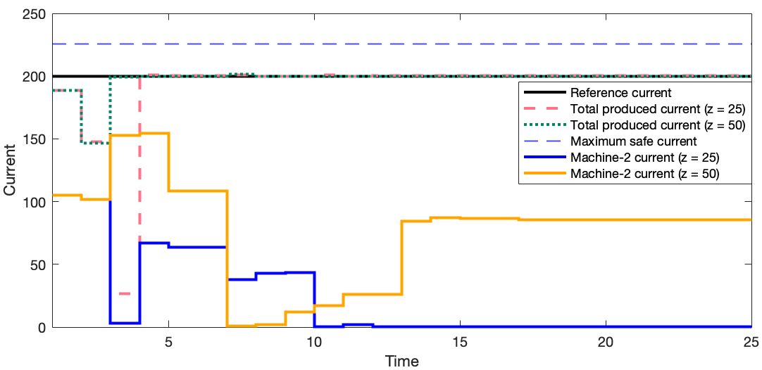
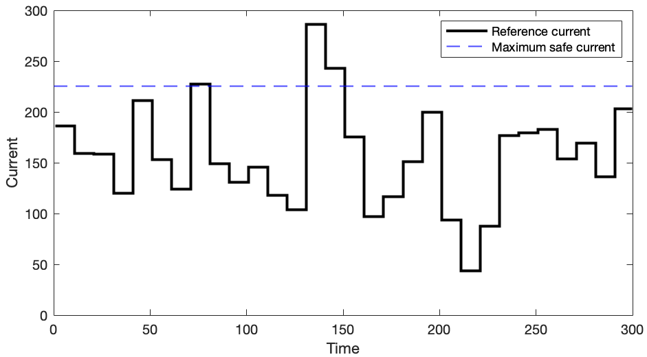
After building the optimization problem, the reference current to follow by ARTEO is generated as in Figure 1. The reference trajectory is designed in such a way that it includes values impossible to reach without violating the safety limit (the black points over the blue dashed line). The aim of this case study is to follow the given reference currents by assigning the torques to the motors while the current to be produced at the decided torque is predicted by the GPs of each motor. Therefore, ARTEO learns the torque-current relationship first from the given safe seed for each motor, then update the GPs of the corresponding motors with its noisy observations at each time step.
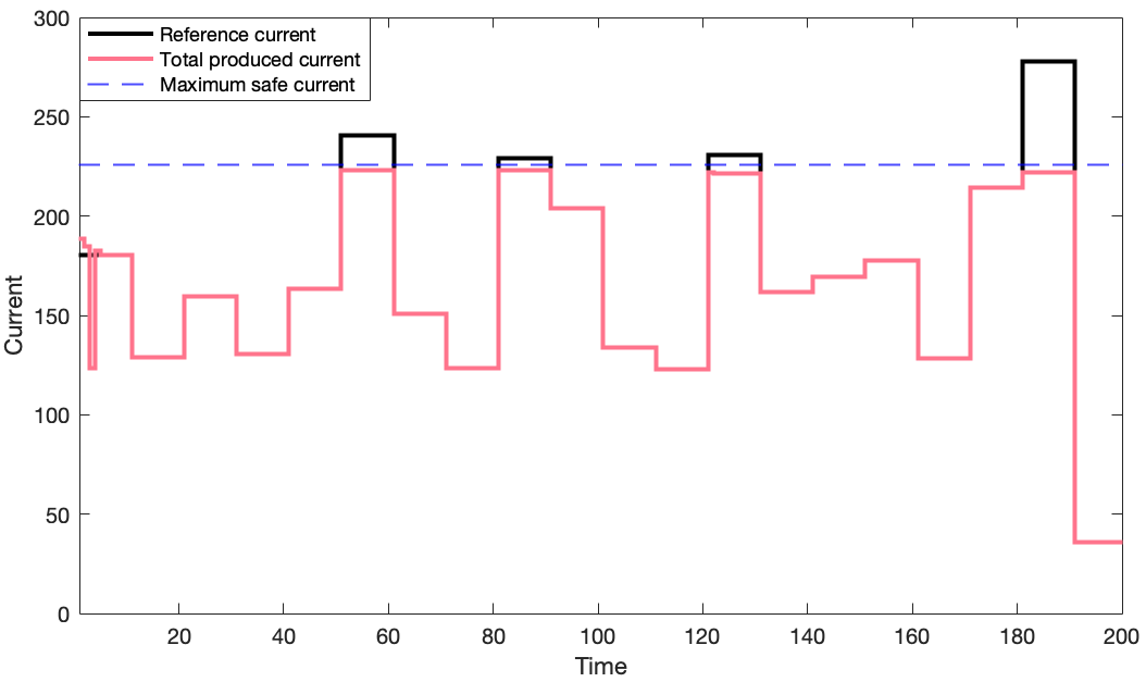
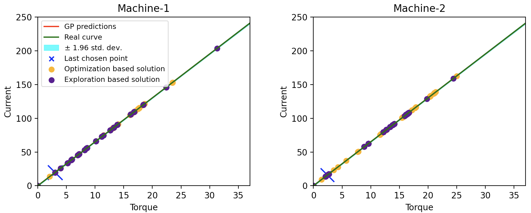
The safe seed of each motor consists of two safe points which are chosen from collected data in the GEM environment. The kernel functions of both GPs are chosen as a squared-exponential kernel with a length scale of 215 (set experimentally). The value of exploration parameter is decided as 25. Hyperparameter optimization techniques for are discussed and employed in this case study in Section B.1.3. The result of the simulation for the reference in Figure 1 is given Figure 2. Figure 2 shows that ARTEO is able to learn the torque-current relationship for given electric motors and optimize the torque values to produce given reference currents after a few time steps without violating the maximum safe current limit for this scenario.
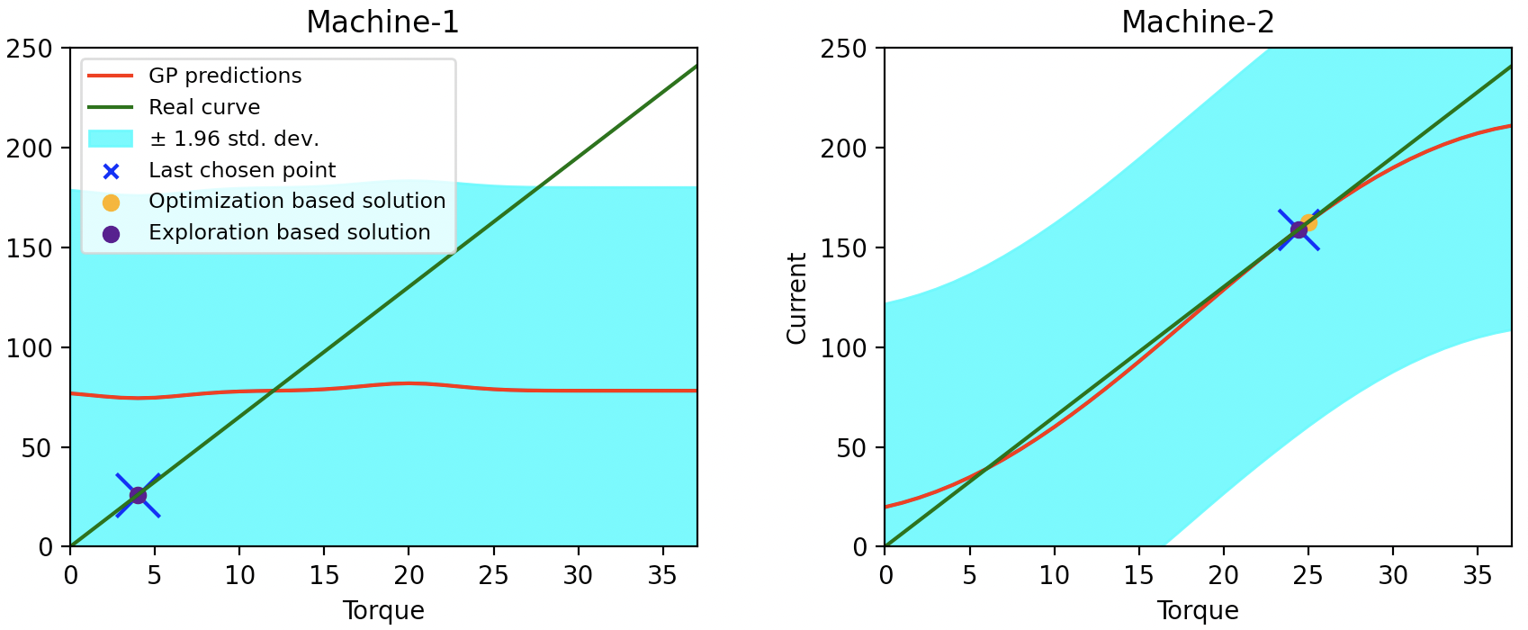
The environment is set to be available for exploration if the reference current of time step is the same as the previous step and this reference is satisfied with a small margin ( 5 A) in the previous step. When exploration starts (second time step) ARTEO prioritizes safe learning for the given value. In the second time step, ARTEO sends Machine-2 to a greater torque which helps decrease uncertainty while sending Machine-1 to a smaller torque to not violate the maximum safe current threshold. The comparison of estimated and real torque-current curves for the second and last time steps of the simulation is given in Figure 3. The effect of the exploration hyperparameter and recommended approaches to set it to an optimal value is discussed with additional experiments in Section B.1.
4.1.2 Comparison with UCB algorithms
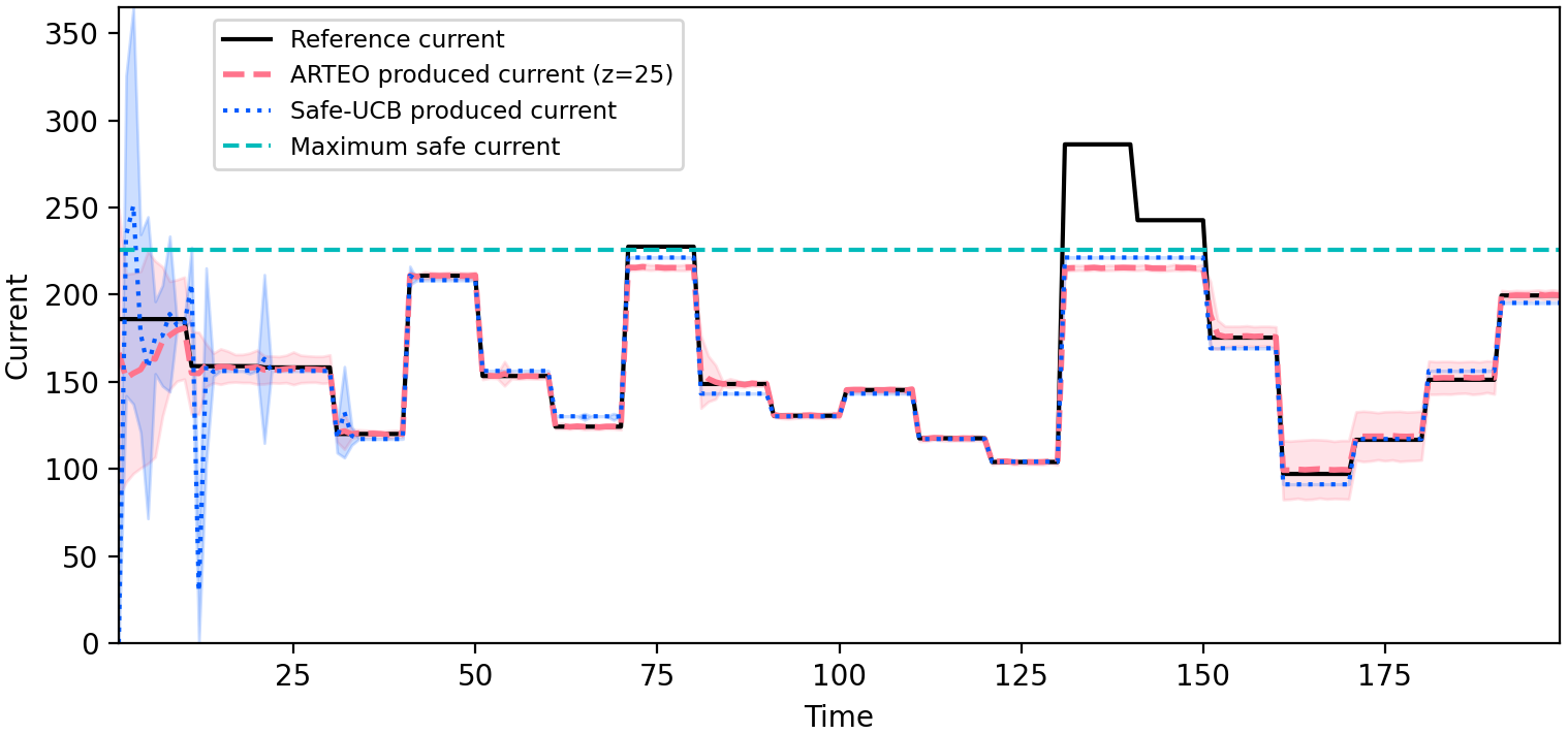
We compare ARTEO with a safety-aware version of GP-UCB algorithm. We implement GP-UCB as in Srinivas et al. (2010) to explore and exploit the decisions that minimize the objective function. Since the functional form is unknown in the original GP-UCB, we develop Safe-UCB without leveraging this information. A main difference between the original GP-UCB and Safe-UCB is that we add another GP to collect data of and learn the unsafe torque values by using the upper confidence bound as in ARTEO. The complete algorithm of Safe-UCB is given in Section B.2. We simulate the reference current value in Figure 4 with 50 different safe seeds. The results show that Safe-UCB tends to violate the safety constraint and operate the electric motors far from optimal values at first explored points due to high standard deviation in its predictions. Even though ARTEO is affected also from the same level of uncertainty at the beginning of the simulation, the standard deviation of its decisions is significantly less than Safe-UCB.
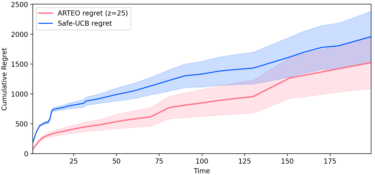
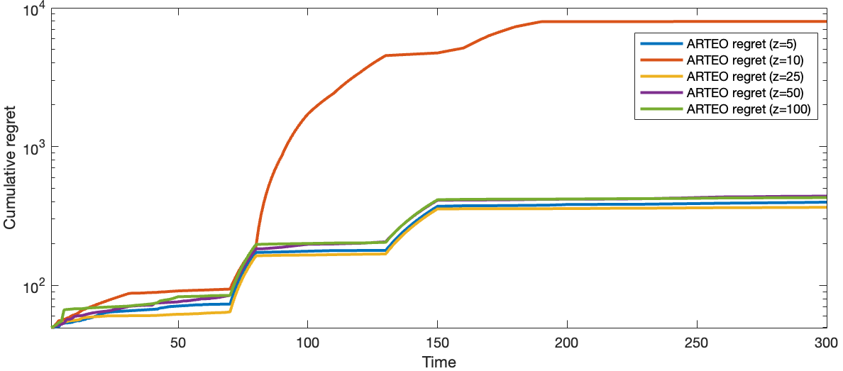
Moreover, Figure 4 demonstrates that while Safe-UCB under or over delivers produced current in several points, ARTEO is more capable to find points that minimize the objective function unless the reference value is unsafe with respect to safety constraint. We further compare the cumulative regret of both algorithms as in Figure 5 by defining the regret at time step ,
| (12) |
Figure 5 shows the superiority of ARTEO to learn the unknown characteristics in a more accurate manner and leverage them in optimization.
4.2 Online Bid Optimization
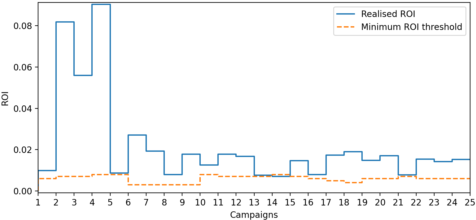
In the second experiment, we investigate the implementation of ARTEO in a multi-dimensional problem of online bid optimization from the advertiser perspective. In bid optimization, the advertiser sets bid values with the aim of achieving high volumes by maximizing the number of shown advertisements and high profitability by maximizing the return-on-investment (ROI) ratio. In most agreements, unsatisfied ROI causes financial losses for advertisers. It becomes more challenging to sustain high ROIs when the number of advertisements increases. Constraining the ROI to remain above a certain threshold is a common approach, however, this method does not guarantee to satisfy the ROI constraint with zero violation (Castiglioni et al., 2022). ROI is measured by the revenues and costs, which are unknown to the bidding algorithms and brings uncertainty to the online bid optimization problem. Therefore, safe optimization algorithms could be useful to set bid values under the uncertainty of the revenues.
We apply ARTEO to the iPinYou dataset (Liao et al., 2014). This dataset has been released by a leading DSP (Demand-Side Platform) in China and consists of relevant information for personalized ads such as creative metadata, interests of users, and advertisement slot properties with decided bid price by their internal algorithm. It has been widely used as a benchmark to evaluate the performance of real-time-bidding algorithms (Zhang et al., 2016; Ren et al., 2017; Wang et al., 2017). We simulate our approach by creating different campaign subsets from the original data, and for each campaign , we minimize the following cost function
| (13) |
where denotes the ad number in the campaign, is the mean prediction of GP for the th advertisement to get a click with set bid values , and is the mean prediction of GP for the bid price of th ad in campaign based on previous observations. The fixed budget constraint for number of ads in campaign is formulated as
| (14) |
The safe ROI constraint is constructed for the threshold for the campaign as follows
| (15) |
Lastly, the bid values are bounded with non-negativity for all campaigns and for all advertisements .
As opposed to the first experiment, where the changes in optimization goals were driven by changes in current references, an increase in in the online bid optimization example is driven by starting a new campaign. We construct two GPs in this experiment, the first GP learns the bid prices from past observations, and the second one models the impressions, which are represented in binary for clicks. The impressions are traditionally predicted by classifiers due to their binary representation. However, it is possible to cast it as a regression problem where we decide the binary representations after thresholding. Since we use covariance functions of GPs to model uncertainty, we cast it as a regression and guide our RTO with continuous values. The optimization algorithm bids an ad comparatively high when its value is higher than others.
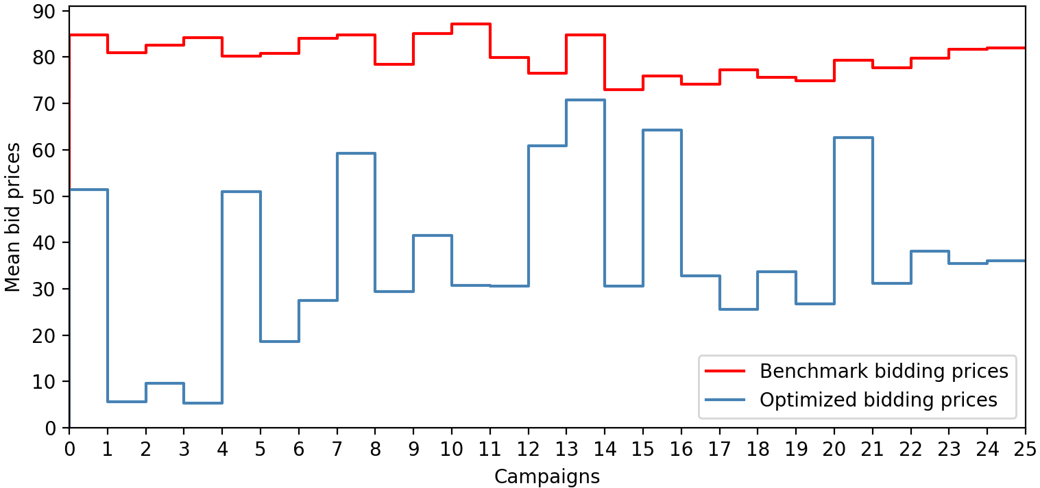
Different feature sets in the dataset are used to compute posteriors based on relevance to the predictions. Further implementation details such as kernel function, hyperparameters and safety limits could be found in Section B.3. The results of the simulation are given in Figure 6 and Figure 7. Our approach remains above the safety threshold while proposing lower bid prices compared to the given bid prices of the algorithm in Liao et al. (2014).
5 CONCLUSIONS
In this work, we investigate real-time optimization of sequential-decision making in a safety-critical system under uncertainty due to partially known characteristics. We propose a safe exploration and optimization algorithm which follows the optimization goals and does exploration without violating the constraints. We adaptively control the contribution of exploration via the uncertainty term in the cost function. We demonstrate the applicability of our approach to real-world case studies. Our algorithm is able to model the unknown parameters in both applications and satisfy the optimization goals and safety constraints.
References
- Bubeck et al. (2012) Sébastien Bubeck, Nicolo Cesa-Bianchi, et al. Regret analysis of stochastic and nonstochastic multi-armed bandit problems. Foundations and Trends® in Machine Learning, 5(1):1–122, 2012.
- Lai and Robbins (1985) T.L Lai and Herbert Robbins. Asymptotically efficient adaptive allocation rules. Advances in Applied Mathematics, 6(1):4–22, 1985. ISSN 0196-8858. doi: https://doi.org/10.1016/0196-8858(85)90002-8. URL https://www.sciencedirect.com/science/article/pii/0196885885900028.
- Lattimore and Szepesvári (2020) Tor Lattimore and Csaba Szepesvári. Stochastic Bandits with Finitely Many Arms, page 73–74. Cambridge University Press, 2020. doi: 10.1017/9781108571401.008.
- Dani et al. (2008) Varsha Dani, Thomas P Hayes, and Sham M Kakade. Stochastic linear optimization under bandit feedback. 2008.
- Bubeck et al. (2009) Sébastien Bubeck, Rémi Munos, Gilles Stoltz, and Csaba Szepesvári. Online optimization in x-armed bandits. Advances in Neural Information Processing Systems 21 - Proceedings of the 2008 Conference, pages 201–208, 01 2009.
- Srinivas et al. (2010) Niranjan Srinivas, Andreas Krause, Sham M. Kakade, and Matthias W. Seeger. Gaussian process optimization in the bandit setting: No regret and experimental design. In ICML, 2010.
- Rasmussen (2004) Carl Edward Rasmussen. Gaussian Processes in Machine Learning, pages 63–71. Springer Berlin Heidelberg, Berlin, Heidelberg, 2004. ISBN 978-3-540-28650-9. doi: 10.1007/978-3-540-28650-9_4. URL https://doi.org/10.1007/978-3-540-28650-9_4.
- Schreiter et al. (2015) Jens Schreiter, Duy Nguyen-Tuong, Mona Eberts, Bastian Bischoff, Heiner Markert, and Marc Toussaint. Safe exploration for active learning with Gaussian processes. pages 133–149, 09 2015. ISBN 978-3-319-23460-1. doi: 10.1007/978-3-319-23461-8_9.
- Turchetta et al. (2016) Matteo Turchetta, Felix Berkenkamp, and Andreas Krause. Safe exploration in finite markov decision processes with Gaussian processes. In D. Lee, M. Sugiyama, U. Luxburg, I. Guyon, and R. Garnett, editors, Advances in Neural Information Processing Systems, volume 29. Curran Associates, Inc., 2016. URL https://proceedings.neurips.cc/paper/2016/file/9a49a25d845a483fae4be7e341368e36-Paper.pdf.
- Wachi et al. (2018) Akifumi Wachi, Yanan Sui, Yisong Yue, and Masahiro Ono. Safe exploration and optimization of constrained MDPs using Gaussian processes. In Proceedings of the Thirty-Second AAAI Conference on Artificial Intelligence and Thirtieth Innovative Applications of Artificial Intelligence Conference and Eighth AAAI Symposium on Educational Advances in Artificial Intelligence, AAAI’18/IAAI’18/EAAI’18. AAAI Press, 2018. ISBN 978-1-57735-800-8.
- Turchetta et al. (2019) Matteo Turchetta, Felix Berkenkamp, and Andreas Krause. Safe exploration for interactive machine learning. Advances in Neural Information Processing Systems, 32, 2019.
- Sui et al. (2015) Yanan Sui, Alkis Gotovos, Joel W. Burdick, and Andreas Krause. Safe exploration for optimization with Gaussian processes. In Proceedings of the 32nd International Conference on International Conference on Machine Learning - Volume 37, ICML’15, page 997–1005. JMLR.org, 2015.
- Berkenkamp et al. (2016) Felix Berkenkamp, Angela P. Schoellig, and Andreas Krause. Safe controller optimization for quadrotors with Gaussian processes. In 2016 IEEE International Conference on Robotics and Automation (ICRA), pages 491–496, 2016. doi: 10.1109/ICRA.2016.7487170.
- Kabzan et al. (2019) Juraj Kabzan, Lukas Hewing, Alexander Liniger, and Melanie N. Zeilinger. Learning-based model predictive control for autonomous racing. IEEE Robotics and Automation Letters, 4(4):3363–3370, 2019. doi: 10.1109/LRA.2019.2926677.
- Agrawal and Goyal (2013) Shipra Agrawal and Navin Goyal. Thompson sampling for contextual bandits with linear payoffs. In Proceedings of the 30th International Conference on International Conference on Machine Learning - Volume 28, ICML’13, page III–1220–III–1228. JMLR.org, 2013.
- Naysmith and Douglas (2008) Matthew R. Naysmith and Peter L. Douglas. Review of real time optimization in the chemical process industries. Developments in Chemical Engineering and Mineral Processing, 3:67–87, 2008.
- Petsagkourakis et al. (2021) Panagiotis Petsagkourakis, Benoit Chachuat, and Ehecatl Antonio del Rio-Chanona. Safe real-time optimization using multi-fidelity Gaussian processes. In 2021 60th IEEE Conference on Decision and Control (CDC), page 6734–6741. IEEE Press, 2021. doi: 10.1109/CDC45484.2021.9683599. URL https://doi.org/10.1109/CDC45484.2021.9683599.
- Zhang et al. (2022) Duo Zhang, Kexin Wang, Zuhua Xu, Anjan K. Tula, Zhijiang Shao, Zhengjiang Zhang, and Lorenz T. Biegler. Generalized parameter estimation method for model-based real-time optimization. Chemical Engineering Science, 258:117754, 2022. ISSN 0009-2509. doi: https://doi.org/10.1016/j.ces.2022.117754. URL https://www.sciencedirect.com/science/article/pii/S0009250922003384.
- Fu and Levine (2021) Justin Fu and Sergey Levine. Offline model-based optimization via normalized maximum likelihood estimation. ArXiv, abs/2102.07970, 2021.
- Sui et al. (2018) Yanan Sui, Vincent Zhuang, Joel Burdick, and Yisong Yue. Stagewise safe Bayesian optimization with Gaussian processes. In 35th International Conference on Machine Learning, pages 4781–4789. PMLR, 2018.
- Hanche-Olsen and Holden (2010) Harald Hanche-Olsen and Helge Holden. The kolmogorov–riesz compactness theorem. Expositiones Mathematicae, 28(4):385–394, 2010. ISSN 0723-0869. doi: https://doi.org/10.1016/j.exmath.2010.03.001. URL https://www.sciencedirect.com/science/article/pii/S0723086910000034.
- Hewitt (1948) Edwin Hewitt. Rings of real-valued continuous functions. i. Transactions of the American Mathematical Society, 64(1):45–99, 1948. ISSN 00029947. URL http://www.jstor.org/stable/1990558.
- Sriperumbudur et al. (2011) Bharath K. Sriperumbudur, Kenji Fukumizu, and Gert R.G. Lanckriet. Universality, characteristic kernels and RKHS embedding of measures. Journal of Machine Learning Research, 12(70):2389–2410, 2011. URL http://jmlr.org/papers/v12/sriperumbudur11a.html.
- Scholkopf and Smola (2001) Bernhard Scholkopf and Alexander J. Smola. Learning with Kernels: Support Vector Machines, Regularization, Optimization, and Beyond. MIT Press, Cambridge, MA, USA, 2001. ISBN 0262194759.
- Jiao et al. (2022) Junjie Jiao, Alexandre Capone, and Sandra Hirche. Backstepping tracking control using Gaussian processes with event-triggered online learning. IEEE Control Systems Letters, 6:3176–3181, 2022.
- Berkenkamp et al. (2019) Felix Berkenkamp, Angela P Schoellig, and Andreas Krause. No-regret Bayesian optimization with unknown hyperparameters. arXiv preprint arXiv:1901.03357, 2019.
- Chowdhury and Gopalan (2017) Sayak Ray Chowdhury and Aditya Gopalan. On kernelized multi-armed bandits. In International Conference on Machine Learning, pages 844–853. PMLR, 2017.
- Hensman et al. (2013) James Hensman, Nicolo Fusi, and Neil D. Lawrence. Gaussian processes for big data. In Proceedings of the Twenty-Ninth Conference on Uncertainty in Artificial Intelligence, UAI’13, page 282–290, Arlington, Virginia, USA, 2013. AUAI Press.
- Chen et al. (2013) Jie Chen, Nannan Cao, Kian Hsiang Low, Ruofei Ouyang, Colin Tan, and Patrick Jaillet. Parallel Gaussian process regression with low-rank covariance matrix approximations. Uncertainty in Artificial Intelligence - Proceedings of the 29th Conference, UAI 2013, 05 2013.
- Liu et al. (2020) Haitao Liu, Yew Ong, Xiaobo Shen, and Jianfei Cai. When Gaussian process meets big data: A review of scalable GPs. IEEE Transactions on Neural Networks and Learning Systems, PP:1–19, 01 2020. doi: 10.1109/TNNLS.2019.2957109.
- Schittkowski (1986) Klaus Schittkowski. NLPQL: A Fortran subroutine solving constrained nonlinear programming problems. Annals of Operations Research, 5:485–500, 1986.
- Potra and Wright (2000) Florian A. Potra and Stephen J. Wright. Interior-point methods. Journal of Computational and Applied Mathematics, 124(1):281–302, 2000. ISSN 0377-0427. doi: https://doi.org/10.1016/S0377-0427(00)00433-7. URL https://www.sciencedirect.com/science/article/pii/S0377042700004337. Numerical Analysis 2000. Vol. IV: Optimization and Nonlinear Equations.
- Ivorra et al. (2015) Benjamin Ivorra, Bijan Mohammadi, and Angel Ramos. A multi-layer line search method to improve the initialization of optimization algorithms. European Journal of Operational Research, 247:711–720, 12 2015. doi: 10.1016/j.ejor.2015.06.044.
- Traue et al. (2022) Arne Traue, Gerrit Book, Wilhelm Kirchgässner, and Oliver Wallscheid. Toward a reinforcement learning environment toolbox for intelligent electric motor control. IEEE Transactions on Neural Networks and Learning Systems, 33(3):919–928, 2022. doi: 10.1109/TNNLS.2020.3029573.
- Liao et al. (2014) Hairen Liao, Lingxiao Peng, Zhenchuan Liu, and Xuehua Shen. iPinYou global RTB bidding algorithm competition dataset. In Proceedings of the Eighth International Workshop on Data Mining for Online Advertising, pages 1–6, 2014.
- Castiglioni et al. (2022) Matteo Castiglioni, Alessandro Nuara, Giulia Romano, Giorgio Spadaro, Francesco Trovò, and Nicola Gatti. Safe online bid optimization with return-on-investment and budget constraints subject to uncertainty. ArXiv, abs/2201.07139, 2022.
- Zhang et al. (2016) Weinan Zhang, Tianxiong Zhou, Jun Wang, and Jian Xu. Bid-aware gradient descent for unbiased learning with censored data in display advertising. In Proceedings of the 22nd ACM SIGKDD international conference on Knowledge discovery and data mining, pages 665–674, 2016.
- Ren et al. (2017) Kan Ren, Weinan Zhang, Ke Chang, Yifei Rong, Yong Yu, and Jun Wang. Bidding machine: Learning to bid for directly optimizing profits in display advertising. IEEE Transactions on Knowledge and Data Engineering, 30(4):645–659, 2017.
- Wang et al. (2017) Jun Wang, Weinan Zhang, Shuai Yuan, et al. Display advertising with real-time bidding (RTB) and behavioural targeting. Foundations and Trends® in Information Retrieval, 11(4-5):297–435, 2017.
- LaValle et al. (2004) Steven M LaValle, Michael S Branicky, and Stephen R Lindemann. On the relationship between classical grid search and probabilistic roadmaps. The International Journal of Robotics Research, 23(7-8):673–692, 2004.
- Frazier (2018) Peter I. Frazier. A tutorial on Bayesian optimization. 2018. doi: 10.48550/ARXIV.1807.02811. URL https://arxiv.org/abs/1807.02811.
- De Ath et al. (2021) George De Ath, Richard M. Everson, and Jonathan E. Fieldsend. Asynchronous -greedy Bayesian optimisation. In Cassio de Campos and Marloes H. Maathuis, editors, Proceedings of the Thirty-Seventh Conference on Uncertainty in Artificial Intelligence, volume 161 of Proceedings of Machine Learning Research, pages 578–588. PMLR, 27–30 Jul 2021. URL https://proceedings.mlr.press/v161/de-ath21a.html.
- Letham and Bakshy (2019) Benjamin Letham and Eytan Bakshy. Bayesian optimization for policy search via online-offline experimentation. Journal of Machine Learning Research, 20(145):1–30, 2019. URL http://jmlr.org/papers/v20/18-225.html.
Appendix A Proofs
A.1 Proof of Lemma 2.4
Let and where . Given is monotonically related to , is in a known functional form of with a known value of , and :
-
•
if is monotonically related to .
-
•
if is inversely monotonically related to .
Proof.
Let , and are continuous functions over domain . We assume has a known functional form as defined by algebraic operations over known and unknown , which is modelled by using Gaussian processes. It is given that is monotonically related to .
-
1.
Consider the first case in Lemma 2.4 as for any such that (Definition 2.2). For chosen such that
(16) With given is monotonically related to :
(17) Let and . By substituting terms in Equation 17, we obtain
(18) We can replace with any that satisfies . Thus, we have:
(19) -
2.
Consider the second case in Lemma 2.4 as for any such that (Definition 2.3). For chosen such that
(20) With given is inversely monotonically related to :
(21) Let and . By substituting terms in Equation 21, we obtain
(22) We can replace with any that satisfies . Thus, we have:
(23)
∎
A.2 Proof of Theorem 2.5
Suppose that and are continuous on compact set , the functional form of is known and is monotonically related to where is modelled from a GP through noisy observations and is a -sub-Gaussian noise for a constant at each iteration . For a known value of , the maximum and minimum values of lie on the upper and lower confidence bounds of the Gaussian process obtained for which are computed as in Lemma 2.4. For a chosen and allowed failure probability as in Equation 4,
-
•
if is monotonically related to
-
•
if is inversely monotonically related to
Proof.
Theorem 2 by Chowdhury and Gopalan [2017] shows that the following holds with probability at least :
| (24) |
by choosing a as in Equation 4 under the assumptions of and is -sub-Gaussian for all (for proof, see Theorem 2 of [Chowdhury and Gopalan, 2017]). We can extract the inequality from absolute value as in the following
| (25) |
Define and as
| (26) |
| (27) |
Then, plug and into Equation 25 and obtain the following with probability
| (28) |
By the proof of Lemma 2.4, we can reflect this inequality to since is defined as monotonically related to . Thus following statements hold with probability,
-
•
if is monotonically related to ,
-
•
if is inversely monotonically related to .
∎
Appendix B Experiment Details
We have constrained nonlinear problems in the experiments section, and we choose interior-point and sequential-least square programming (SLSQP) algorithms to solve our first and second problems, respectively.
B.1 Implementation of ARTEO to Electric Motor Current Optimization
B.1.1 Electric Motor Simulation Environment Details
Gym-Electric-Motor (GEM) is an environment that includes the simulation of different types of electric motors with adjustable parameters such as load, speed, current, torque, etc. to train reinforcement learning agents or build model predictive control solutions to control the current, torque or speed for a given reference. In electric motors, the operation range is limited by nominal values of variables to prevent motor damage. Furthermore, there are also safety limits for some parameters, such as the maximum safe current limit to avoid excessive heat generation.
| Electric Motor | ||||
|---|---|---|---|---|
| Machine-1 | 0.016 | 1.9e-05 | 0.165 | 0.025 |
| Machine-2 | 0.01 | 1.5e-05 | 0.165 | 0.025 |
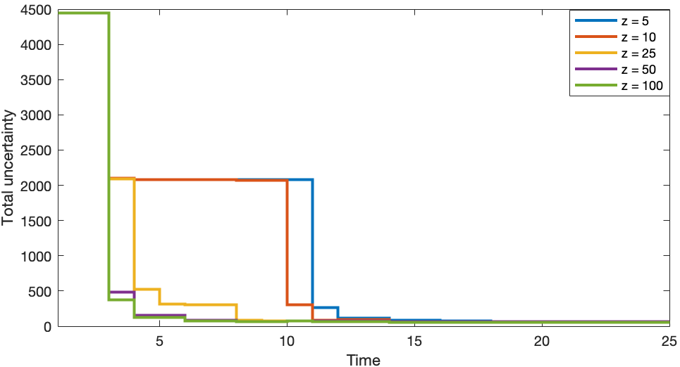
B.1.2 The Impact of Exploration Hyperparameter
The exploration in ARTEO is driven by the hyperparameter. It is possible to create different strategies according to the requirements of the problem by setting different values to this hyperparameter. To demonstrate this, we simulate a constant reference current scenario with different values, as in Figure 8. This figure exhibits that greater values lead to more frequent changes in reference torque values while preserving the ability to satisfy the reference current. It is expected that more frequent changes in the operating points assist in decreasing the total uncertainty in the environment faster. This is demonstrated in Figure 9 for different values for the reference scenario in Figure 8. Hyperparameter optimization methods could be leveraged to choose the value of to achieve minimum regret where regret at time is defined as Equation 12.
B.1.3 Hyperparameter Optimization for
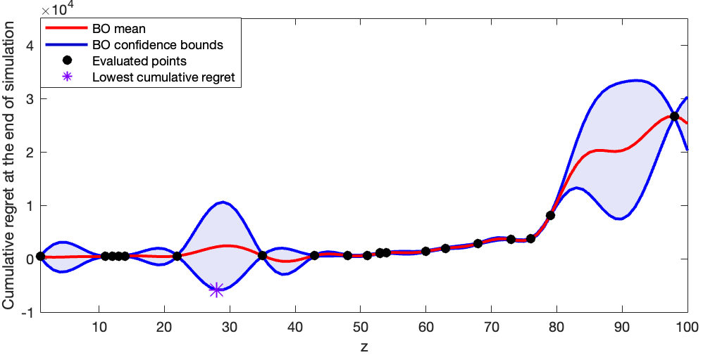
During the implementation of ARTEO to electric motor current optimization, we choose after applying two hyperparameter optimization methods as the grid-search [LaValle et al., 2004] and Bayesian optimization (BO) [Frazier, 2018]. We evaluate different values based on the cumulative regret at the end of the simulation of reference in Figure 10. For grid-search, we evaluate the cumulative regret with taking values of 5, 10, 25, 50, and 100. The results in Figure 11 show that the most suitable value for the given reference is 25 amongst the evaluated values.
As an alternative hyperparameter technique to grid-search, BO is also applied to the simulation of the given reference. BO is an optimization method that builds a surrogate model with evaluations at chosen points and then chooses the next value to be evaluated based on the minimization/maximization of the chosen acquisition function, which is specified as lower confidence bound in our implementation. Further details of BO could be found in Frazier [2018]. We limit the maximum number of evaluations with 35 points and the results in Figure 11 demonstrate that the surrogate model of BO suggests that the minimum cumulative regret at the end of the simulation (of Figure 10) when .
Hyperparameter optimization becomes more challenging in the online learning setup where complete information is not available to do simulation. A suggested hyperparameter optimization method for ARTEO implementation in online learning could be starting with a random value and adjusting it based on replaying the available simulation and optimizing the hyperparameter asynchronously whenever new information is available. Similar hyperparameter optimization techniques for online learning could be found in De Ath et al. [2021] and Letham and Bakshy [2019].
B.2 Implementation of Safe-UCB to Electric Motor Current Optimization
In electric motor current optimization experiments, is calculated as the difference between the given reference current and the total produced current. Thus, we search points that minimize the value of which leads us to use lower confidence bound of by following the optimism principle of Lai and Robbins [1985]. The safety function is defined as the difference between the safety limit value and the total produced current. Hence, the chosen points are safe as long as the value of chosen points remains above zero.
B.3 Environment Details for Online Bid Optimization
The GP of the bid price is initialized with the Matern kernel with = 1.5 and is trained over 143 features whereas the impression GP has the Squared Exponential kernel and 69 features. The safe seeds start with 30 samples, which is higher than our first experiment since this is a higher dimensional problem. As a minimum ROI threshold, 90% of the given benchmark data ROI is set due to having a strict budget and ROI requirements in our setup. We partition the selected subset of the dataset into 25 campaigns. Each campaign has its ROI threshold and budget, which are calculated as Equation 14 and Equation 15.
The algorithm starts with a safe seed set to compute the posteriors of GPs, and then for each campaign, it utilizes the mean and standard deviation of GP posteriors to measure ROI and click probability. During the RTO phase, the higher bid prices for higher estimated click values are encouraged within a fixed budget, and the difference between the predicted bid price by GP and the proposed bid price by RTO for each advertisement is accumulated and introduced as a penalty in the objective function. Thus, the algorithm does not put the entire budget into the highest-valued ad within the campaign. At the end of each campaign, true bid prices and clicks with additive Gaussian noise are used to update the posteriors of GPs. The feedback is given only for ads in the campaign with a non-negative optimized bid price which leads to high standard deviations for non-bid similar ads. The environment becomes available for exploration after spending less than the sum of predicted bid prices and satisfying minimum thresholds in two consecutive campaigns. Hence, is set to = 100 to excite the RTO to take decisions at points that could reduce uncertainty in predictions.