Regret Bounds for Noise-Free Cascaded Kernelized Bandits

Abstract

We consider optimizing a function network in the noise-free grey-box setting with RKHS function classes, where the exact intermediate results are observable. We assume that the structure of the network is known (but not the underlying functions comprising it), and we study three types of structures: (1) chain: a cascade of scalar-valued functions, (2) multi-output chain: a cascade of vector-valued functions, and (3) feed-forward network: a fully connected feed-forward network of scalar-valued functions. We propose a sequential upper confidence bound based algorithm GPN-UCB along with a general theoretical upper bound on the cumulative regret. For the Matérn kernel, we additionally propose a non-adaptive sampling based method along with its theoretical upper bound on the simple regret. We also provide algorithm-independent lower bounds on the simple regret and cumulative regret, showing that GPN-UCB is near-optimal for chains and multi-output chains in broad cases of interest.

1 Introduction

Black-box optimization of an expensive-to-evaluate function based on point queries is a ubiquitous problem in machine learning. Bayesian optimization (or Gaussian process optimization) refers to a class of methods using Gaussian processes (GPs), whose main idea is to place a prior over the unknown function and update the posterior according to point query results. Bayesian optimization has a wide range of applications including parameter tuning (Snoek et al., 2012), experimental design (Griffiths & Hernández-Lobato, 2020), and robotics (Lizotte et al., 2007).

In the literature on Bayesian optimization, the problem of optimizing a real-valued black-box function is usually studied under two settings: (1) Bayesian setting: the target function is sampled from a known GP prior, and (2) non-Bayesian setting: the target function has a low norm in reproducing kernel Hilbert space (RKHS).

In this work, we consider a setting falling “in between” the white-box setting (where the full definition of the target function is known) and the black-box setting, namely, a grey-box setting in which the algorithms can leverage partial internal information of the target function beyond merely the final outputs or even slightly modify the target function (Astudillo & Frazier, 2021b). Existing grey-box optimization methods exploit internal information such as observations of intermediate outputs for composite functions (Astudillo & Frazier, 2019) and lower fidelity but faster approximation of the final output for modifiable functions (Huang et al., 2006). Numerical experiments show that the grey-box methods significantly outperform standard black-box methods (Astudillo & Frazier, 2021b).

Though any real-valued network can be treated as a single black-box function and solved with classical Bayesian optimization methods, we explore the benefits offered by utilizing the network structure information and the exact intermediate results under the noise-free grey-box setting.

1.1 Related Work

Numerous works have proposed Bayesian optimization algorithms for optimizing a single real-valued black-box function under the RKHS setting. For the noisy setting, (Srinivas et al., 2010; Chowdhury & Gopalan, 2017; Gupta et al., 2022) provide a typical cumulative regret ${\widetilde{O}}(\sqrt{T}\gamma_{T})$, where $T$ is the time horizon, $\gamma_{T}$ is the maximum information gain associated to the underlying kernel, and the ${\widetilde{O}}(\cdot)$ notation hides the poly-logarithmic factors. Recently, (Camilleri et al., 2021; Salgia et al., 2021; Li & Scarlett, 2022) achieved cumulative regret ${\widetilde{O}}(\sqrt{T\gamma_{T}})$, which nearly matches algorithm-independent lower bounds for the squared exponential and Matérn kernels (Scarlett et al., 2017; Cai & Scarlett, 2021). For the noise-free setting, (Bull, 2011) achieves a nearly optimal simple regret $O(T^{-\nu/d})$ for the Matérn kernel with smoothness $\nu$. This result implies a two-batch algorithm that uniformly selects $T^{\frac{d}{\nu+d}}$ points in the first batch and repeatedly picks the returned point in the second batch, has cumulative regret $O(T^{\frac{d}{\nu+d}})$. In addition, (Lyu et al., 2019) provides deterministic cumulative regret $O(\sqrt{T\gamma_{T}})$, with the rough idea being to substitute zero noise into the analysis of GP-UCB (Srinivas et al., 2010).

Recently, several Bayesian optimization algorithms for optimizing a composition of multiple functions under the noise-free setting have been proposed. (Nguyen et al., 2016) provides a method for cascade Bayesian optimization; (Astudillo & Frazier, 2019) studies optimizing a composition of a black-box function and a known cheap-to-evaluate function; and (Astudillo & Frazier, 2021a) studies optimizing a network of functions sampled from a GP prior under the grey-box setting. Both (Astudillo & Frazier, 2019) and (Astudillo & Frazier, 2021a) prove the asymptotic consistency of their expected improvement sampling based methods.

The most related work to ours is (Kusakawa et al., 2021), which introduces two confidence bound based algorithms along with their regret guarantees. A detailed comparison regarding problem setup and theoretical performance is provided in Appendix H. In short, we significantly improve certain dependencies in their regret for a UCB-type approach, and we study two new directions – non-adaptive sampling and algorithm-independent lower bounds – that were not considered therein (see Section 1.2 for a summary).

For function networks with $m$ layers, our cumulative regret bounds are expressed in terms of

$$\Sigma_{T}=\max_{i\in[m]}\max_{{\mathbf{z}}_{1},\dots,{\mathbf{z}}_{T}\in\mathcal{X}^{(i)}}\sum_{t=1}^{T}\sigma^{(i)}_{t-1}({\mathbf{z}}_{t}),$$

where $\mathcal{X}^{(i)}$ and $\sigma^{(i)}_{t-1}(\cdot)$ denote the domain and posterior standard deviation of the $i$-th layer respectively. This is a term for general layer-composed networks associated to domains $\mathcal{X}^{(1)},\dots,\mathcal{X}^{(m)}$ and kernel $k$. When $m=1$, the term $\max_{{\mathbf{x}}_{1},\dots,{\mathbf{x}}_{T}\in\mathcal{X}}\sum_{t=1}^{T}\sigma_{t-1}({\mathbf{x}}_{t})$ often appears in the cumulative regret analysis of classic black-box optimization (Srinivas et al., 2010; Lyu et al., 2019; Vakili, 2022). Explicit upper bounds on $\Sigma_{T}$ will be discussed in Section 3.4

1.2 Contributions

We study the problem of optimizing an $m$-layer function network in the noise-free grey-box setting, where the exact intermediate results are observable. We focus on three types of network structures: (1) chain: a cascade of scalar-valued functions, (2) multi-output chain: a cascade of vector-valued functions, and (3) feed-forward network: a fully connected feed-forward network of scalar-valued functions. Then:

• We propose a fully sequential upper confidence bound based algorithm GPN-UCB along with its upper bound on cumulative regret for each network structure.

• We introduce a non-adaptive sampling based method, and provide its theoretical upper bound on the simple regret for the Matérn kernel.

• We provide algorithm-independent lower bounds on the simple regret and cumulative regret for an arbitrary algorithm optimizing any chain, multi-output chain, or feed-forward nework associated to the Matérn kernel. We show that the upper and lower bounds nearly match in broad cases of interest.

Let $d$ denote the dimension of the domain, $d_{\max}$ denote the maximum dimension among all the $m$ layers, and $D_{2,m}$ denote the product of dimensions from the second layer to the last layer. With $B>0$ restricting the magnitude and smoothness of each layer and $L>1$ restricting the slope of each layer, a partial summary of the proposed cumulative regret bounds for the Matérn kernel with smoothness $\nu\geq 1$ when $d\geq\nu$ and $T=\Omega\big{(}(B(cL)^{m-1})^{d/\nu}\big{)}$ for $c=\Theta(1)$ is displayed in Table 1, showing that the upper bounds and the lower bound share the same $BL^{m-1}T^{1-\nu/d}$ dependence when $d=d_{\max}$.

We highlight that to our knowledge, we are the first to attain provably near-optimal scaling (in broad cases of interest), and doing so requires both improving the existing upper bounds (e.g., (Kusakawa et al., 2021)) and attaining novel lower bounds. A full summary of our theoretical results is provided in Appendix G.

Lower bound	$\Omega(B(cL)^{m-1}T^{1-\nu/d})$
Upper bound (chains)	$2^{m+1}BL^{m-1}T^{1-\nu/d}$
Upper bound (multi-output chains)	$5^{m}BL^{m-1}T^{1-\nu/d_{\max}}$
Upper bound (feed-forward networks)	$2^{m+1}\sqrt{D_{2,m}}BL^{m-1}T^{1-\nu/d_{\max}}$

Table 1: Summary of proposed cumulative regret bounds for the Matérn kernel when $d\geq\nu\geq 1$ and $T=\Omega\big{(}(B(cL)^{m-1})^{d/\nu}\big{)}$.

2 Problem Setup

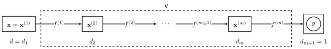
Figure 1: A function network $g$ of $m$ layers with input ${\mathbf{x}}$ and output $y$.

We consider optimizing a real-valued grey-box function $g$ on $\mathcal{X}=[0,1]^{d}$ based on noise-free point queries. (We briefly comment on noisy settings in Section 7.) As shown in Figure 1, the target function $g$ is known to be a network of $m$ unknown layers $f^{(i)}$ with $i\in[m]$. In general, for any input ${\mathbf{x}}\in\mathcal{X}$, the network $g$ has a structure such that

$$\mathbf{x}^{(1)} ={\mathbf{x}},$$

$$\mathbf{x}^{(i+1)} =f^{(i)}(\mathbf{x}^{(i)})\text{ for }i\in[m-1],$$

$$y =g({\mathbf{x}})=f^{(m)}(\mathbf{x}^{(m)})\in{\mathbb{R}},$$

where $\mathbf{x}^{(i)}$ has dimension $d_{i}$ for each $i\in[m]$. The domain of $f^{(i)}$ is $\mathcal{X}^{(i)}$, and the range of $f^{(i)}$ is $\mathcal{X}^{(i+1)}$. For any ${\mathbf{z}}\in\mathcal{X}^{(i)}$, there exists a corresponding ${\mathbf{x}}\in\mathcal{X}$ such that $\mathbf{x}^{(i)}={\mathbf{z}}$.

We aim to find ${\mathbf{x}}^{\ast}=\operatorname*{arg\,max}_{{\mathbf{x}}\in\mathcal{X}}g({\mathbf{x}})$ based on a sequence of point queries up to time horizon $T$. When we query $g$ with input ${\mathbf{x}}_{t}$ at time step $t$, the intermediate noise-free results $\mathbf{x}^{(2)}_{t},\dots,\mathbf{x}^{(m)}_{t}$ and the final noise-free output $y_{t}$ are accessible. We measure the performance using the following two notions:

• Simple regret: With ${\mathbf{x}}_{T}^{\ast}$ being additional point returned after $T$ rounds, the simple regret is defined as $r_{T}^{\ast}=g({\mathbf{x}}^{\ast})-g({\mathbf{x}}_{T}^{\ast})$;

• Cumulative regret: The cumulative regret incurred over $T$ rounds is defined as $R_{T}=\sum_{i=1}^{T}r_{t}$ with $r_{t}=g({\mathbf{x}}^{\ast})-g({\mathbf{x}}_{t})$.

2.1 Kernelized Bandits

We assume $g$ is a composition of multiple constituent functions, for which we consider both scalar-valued functions and vector-valued functions based on a given kernel.

Scalar-valued functions. For a given scalar-valued kernel $k:\mathcal{X}\times\mathcal{X}\to{\mathbb{R}}$, consider a function space $\mathcal{S}_{k}:=\{f(\cdot)=\sum_{i=1}^{n_{0}}a_{i}k(\cdot,{\mathbf{x}}_{i}):n_{0}\in{\mathbb{N}},a_{i}\in{\mathbb{R}},{\mathbf{x}}_{i}\in\mathcal{X}\}$. Then, the reproducing kernel Hilbert space (RKHS) corresponding to kernel $k$, denoted by $\mathcal{H}_{k}$, can be obtained by forming the completion of $\mathcal{S}_{k}$, and the elements in $\mathcal{H}_{k}$ are called scalar-valued kernelized bandits or GP bandits. $\mathcal{H}_{k}$ is equipped with the inner product

$$\langle f,f^{\prime}\rangle_{k}=\sum_{i=1}^{n_{1}}\sum_{j=1}^{n_{2}}a_{i}b_{j}k({\mathbf{x}}_{i},{\mathbf{x}}^{\prime}_{j})$$ (1)

for $f=\sum_{i=1}^{n_{1}}a_{i}k(\cdot,{\mathbf{x}}_{i})$ and $f^{\prime}=\sum_{j=1}^{n_{2}}b_{j}k(\cdot,{\mathbf{x}}^{\prime}_{j})$. This inner product satisfies the reproducing property, such that $\langle f(\cdot),k(\cdot,{\mathbf{x}})\rangle_{k}=f({\mathbf{x}}),\forall{\mathbf{x}}\in\mathcal{X},\forall f\in\mathcal{H}_{k}$. The RKHS norm of $f$ is $\|f\|_{k}=\sqrt{\langle f,f\rangle_{k}}$, and we use $\mathcal{H}_{k}(B):=\{f\in\mathcal{H}_{k}:\|f\|_{k}\leq B\}$ to denote the set of functions whose RKHS norm is upper bounded by some known constant $B>0$. In this work, we mainly focus on the Matérn kernel:

$$k_{\text{Mat\'{e}rn}}({\mathbf{x}},{\mathbf{x}}^{\prime}) =\frac{2^{1-\nu}}{\Gamma(\nu)}\Bigg{(}\frac{\sqrt{2\nu}d_{{\mathbf{x}},{\mathbf{x}}^{\prime}}}{l}\Bigg{)}^{\nu}B_{\nu}\Bigg{(}\frac{\sqrt{2\nu}d_{{\mathbf{x}},{\mathbf{x}}^{\prime}}}{l}\Bigg{)},$$

where $d_{{\mathbf{x}},{\mathbf{x}}^{\prime}}=\|{\mathbf{x}}-{\mathbf{x}}^{\prime}\|_{2}$, $l>0$ denotes the length-scale, $\nu>0$ is a smoothness parameter, $\Gamma$ is the Gamma function, and $B_{\nu}$ is the modified Bessel function.

Vector-valued functions. An operator-valued kernel $\Gamma:\mathcal{X}\times\mathcal{X}\to{\mathbb{R}}^{n\times n}$ is called a multi-task kernel on $\mathcal{X}$ if $\Gamma(\cdot,\cdot)$ is symmetric positive definite. Moreover, a single-task kernel with $n=1$ recovers a scalar-valued kernel. For a given multi-task kernel $\Gamma$, similarly to the scalar-valued kernels, there exists an RKHS of vector-valued functions $\mathcal{H}_{\Gamma}$, which is the completion of $\mathcal{S}_{\Gamma}:=\{f(\cdot)=\sum_{i=1}^{n_{0}}\Gamma(\cdot,{\mathbf{x}}_{i}){\mathbf{a}}_{i}:n_{0}\in{\mathbb{N}},{\mathbf{a}}_{i}\in{\mathbb{R}}^{n},{\mathbf{x}}_{i}\in\mathcal{X}\}$. The elements in $\mathcal{H}_{\Gamma}$ are called vector-valued kernelized bandits, and $\mathcal{H}_{\Gamma}$ is equipped with the inner product (Carmeli et al., 2006)

$$\langle f,f^{\prime}\rangle_{\Gamma}=\sum_{i=1}^{n_{1}}\sum_{j=1}^{n_{2}}\langle\Gamma({\mathbf{x}}_{i},{\mathbf{x}}_{j}^{\prime}){\mathbf{a}}_{i},{\mathbf{b}}_{j}\rangle$$ (2)

for $f=\sum_{i=1}^{n_{1}}\Gamma(\cdot,{\mathbf{x}}_{i}){\mathbf{a}}_{i}$ and $f^{\prime}=\sum_{j=1}^{n_{2}}\Gamma(\cdot,{\mathbf{x}}^{\prime}_{j}){\mathbf{b}}_{i}$. This inner product satisfies the reproducing property, such that $\langle f(\cdot),\Gamma(\cdot,{\mathbf{x}}){\mathbf{v}}\rangle_{\Gamma}=\langle f({\mathbf{x}}),{\mathbf{v}}\rangle_{2},\forall{\mathbf{x}}\in\mathcal{X},\forall{\mathbf{v}}\in{\mathbb{R}}^{n},\forall f\in\mathcal{H}_{\Gamma}.$ The RKHS norm of $f\in\mathcal{H}_{\Gamma}$ is $\|f\|_{\Gamma}=\sqrt{\langle f,f\rangle_{\Gamma}}$, and we focus on $\mathcal{H}_{\Gamma}(B):=\{f\in\mathcal{H}_{\Gamma}:\|f\|_{\Gamma}\leq B\}$ containing functions with norm at most $B>0$. We will often pay particular attention to the Matérn kernel $\Gamma_{\text{Mat\'{e}rn}}(\cdot,\cdot)=k_{\text{Mat\'{e}rn}}(\cdot,\cdot){\mathbf{I}}$, where $k_{\text{Mat\'{e}rn}}$ is the scalar-valued Matérn kernel and ${\mathbf{I}}$ is the identity matrix of size $n$.

Surrogate GP model. As is common in kernelized bandit problems, our algorithms employ a surrogate Bayesian GP model for $f\in\mathcal{H}_{k}(B)$. For $f$ sampled from the prior with zero mean and kernel $k$, given a sequence of points $({\mathbf{x}}_{1},\dots,{\mathbf{x}}_{t})$ and their noise-free observations $\mathbf{y}_{t}=(y_{1},\dots,y_{t})$ up to time $t$, the posterior distribution of $f$ is a GP with mean and variance given by (Rasmussen & Williams, 2006)

$$\mu_{t}({\mathbf{x}}) =\mathbf{k}_{t}({\mathbf{x}})^{T}\mathbf{K}_{t}^{-1}\mathbf{y}_{t}$$ (3)

$$\sigma_{t}({\mathbf{x}})^{2} =k({\mathbf{x}},{\mathbf{x}})-\mathbf{k}_{t}({\mathbf{x}})^{T}\mathbf{K}_{t}^{-1}\mathbf{k}_{t}({\mathbf{x}}),$$ (4)

where $\mathbf{k}_{t}({\mathbf{x}})=[k({\mathbf{x}},{\mathbf{x}}_{i})]_{i=1}^{t}\in{\mathbb{R}}^{t\times 1}$ and $\mathbf{K}_{t}=[k({\mathbf{x}}_{i},{\mathbf{x}}_{j})]_{i,j=1}^{t}\in{\mathbb{R}}^{t\times t}$. The following lemma shows that the posterior confidence region defined with parameter $B$ is always deterministically valid.

Lemma 1.

(Kanagawa et al., 2018, Corollary 3.11) For $f\in\mathcal{H}_{k}(B)$, let $\mu_{t}({\mathbf{x}})$ and $\sigma_{t}({\mathbf{x}})^{2}$ denote the posterior mean and variance based on $t$ points $({\mathbf{x}}_{1},\dots,{\mathbf{x}}_{t})$ and their noise-free observations $(y_{1},\dots,y_{t})$ using (3) and (4). Then, it holds for all ${\mathbf{x}}\in\mathcal{X}$ that

$$|f({\mathbf{x}})-\mu_{t}({\mathbf{x}})|\leq B\sigma_{t}({\mathbf{x}}).$$

We also impose a surrogate GP model for functions in $\mathcal{H}_{\Gamma}(B)$. The posterior mean and variance matrix based on $({\mathbf{x}}_{1},\dots,{\mathbf{x}}_{t})$ and their noise-free observations $Y_{t}=({\mathbf{y}}_{1},\dots,{\mathbf{y}}_{t})$ are given by (Chowdhury & Gopalan, 2021)

$$\mu_{t}({\mathbf{x}}) =G_{t}({\mathbf{x}})^{T}G_{t}^{-1}Y_{t},$$ (5)

$$\Gamma_{t}({\mathbf{x}},{\mathbf{x}}) =\Gamma({\mathbf{x}},{\mathbf{x}})-G_{t}({\mathbf{x}})^{T}G_{t}^{-1}G_{t}({\mathbf{x}}),$$ (6)

where $G_{t}({\mathbf{x}})=[\Gamma({\mathbf{x}},{\mathbf{x}}_{i})]_{i=1}^{t}\in{\mathbb{R}}^{nt\times n}$, $G_{t}=[\Gamma({\mathbf{x}}_{i},{\mathbf{x}}_{j})]_{i,j=1}^{t}\in{\mathbb{R}}^{nt\times nt}$, and $Y_{t}=[{\mathbf{y}}_{i}]_{i=1}^{t}\in{\mathbb{R}}^{nt\times 1}$. With $\|\cdot\|_{2}$ denoting the spectral norm of a matrix, the following lemma provides a deterministic confidence region.

Lemma 2.

For $f\in\mathcal{H}_{\Gamma}(B)$, let $\mu_{t}({\mathbf{x}})$ and $\Gamma_{t}({\mathbf{x}},{\mathbf{x}})$ denote the posterior mean and variance based on $t$ points $({\mathbf{x}}_{1},\dots,{\mathbf{x}}_{t})$ and their noise-free observations $({\mathbf{y}}_{1},\dots,{\mathbf{y}}_{t})$ using (5) and (6). Then, it holds for all ${\mathbf{x}}\in\mathcal{X}$ that

$$\|f({\mathbf{x}})-\mu_{t}({\mathbf{x}})\|_{2}\leq B\|\Gamma_{t}({\mathbf{x}},{\mathbf{x}})\|_{2}^{1/2}.$$

The proof is given in Appendix A.

2.2 Lipschitz Continuity

We also assume that each constituent function in the network $g$ is Lipschitz continuous. For a constant $L>1$, we denote by $\mathcal{F}(L)$ the set of functions such that

$$\mathcal{F}(L)=\{f:\|f({\mathbf{x}})-f({\mathbf{x}}^{\prime})\|_{2}\leq L\|{\mathbf{x}}-{\mathbf{x}}^{\prime}\|_{2},\forall{\mathbf{x}},{\mathbf{x}}^{\prime}\},$$

where $L$ is called the Lipschitz constant. This is a mild assumption, as (Lee et al., 2022) has shown that Lipschitz continuity is a guarantee for functions in $\mathcal{H}_{k}(B)$ for the commonly-used squared exponential kernel and Matérn kernel with smoothness $\nu>1$.

2.3 Network structures.

Figure 2: A chain with $m=3$, where $\{f^{(i)}\}_{i=1}^{3}$ are scalar-valued functions.

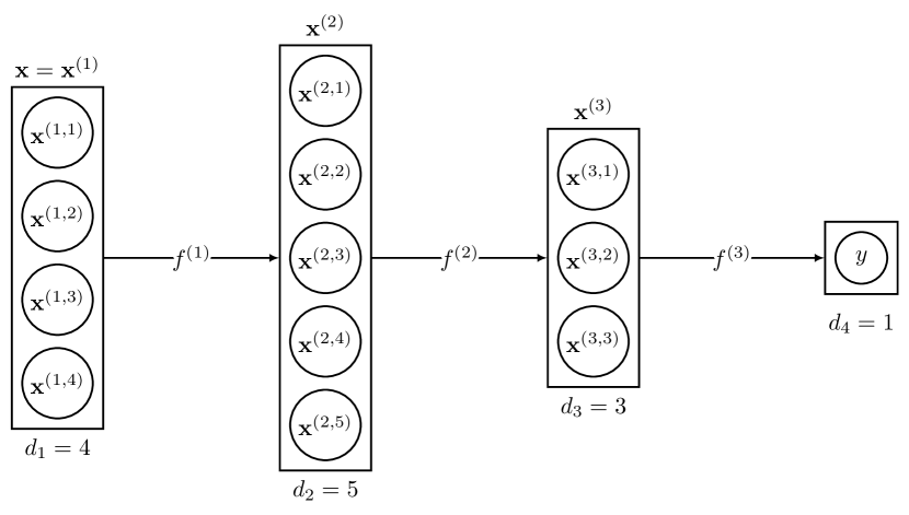
Figure 3: A multi-output chain with $m=3$, where $\{f^{(i)}\}_{i=1}^{3}$ are vector-valued functions.

Figure 4: A feed-forward network with $m=3$, where $f^{(i,j)}$ is a scalar-valued function for each $i\in[3],j\in[d_{i+1}]$.

In this work, we consider three types of network structure for $g$:

• Chain: For a scalar-valued kernel $k$, a chain is a cascade of scalar-valued functions. Specifically, $d_{1}\geq 1$, $d_{2}=d_{3}=\cdots=d_{m}=1$, and $f^{(i)}\in\mathcal{H}_{k}(B)\cap\mathcal{F}(L)$ for each $i\in[m]$. An example is given in Figure 2.

• Multi-output chain: For an operator-valued kernel $\Gamma$, a multi-output chain is a cascade of vector-valued functions. Specifically, $d_{i}\geq 1$ and $f^{(i)}\in\mathcal{H}_{\Gamma}(B)\cap\mathcal{F}(L)$ for each $i\in[m]$. An example is given in Figure 3.

• Feed-forward network: For a scalar-valued kernel $k$, a feed-forward network is a fully-connected feed-forward network of scalar-valued functions. Specifically, $d_{i}\geq 1$ and $f^{(i)}({\mathbf{z}})=[f^{(i,j)}({\mathbf{z}})]_{j=1}^{d_{i+1}}$ with $f^{(i,j)}\in\mathcal{H}_{k}(B)\cap\mathcal{F}(L)$ for each $i\in[m],j\in[d_{i+1}]$. An example is given in Figure 4.

For all the cases above, the overall network $g$ is scalar-valued with the dimension of the final output $y$ being $d_{m+1}=1$.

3 GPN-UCB Algorithm and Regret Bounds

Algorithm 1 GPN-UCB (Gaussian Process Network - Upper Confidence Bound)

1:  for all $t\leftarrow 1,2,\dots,T$ do

2:     Select ${\mathbf{x}}_{t}\leftarrow\operatorname*{arg\,max}_{{\mathbf{x}}\in\mathcal{X}}\mathrm{UCB}_{t-1}({\mathbf{x}})$

3:     Obtain observations $\mathbf{x}^{(2)}_{t},\dots,\mathbf{x}^{(m)}_{t},$ and $y_{t}$.

4:     Compute $\mathrm{UCB}_{t}$ using (13), (17), or (22) based on $\{\mathbf{x}^{(1)}_{s},\dots,\mathbf{x}^{(m)}_{s},y_{s}\}_{s=1}^{t}$.

5:  end for

In this section, we propose a fully sequential algorithm GPN-UCB (see Algorithm 1) for chains, multi-output chains, and feed-forward networks. The algorithm works with structure-specific upper confidence bounds. Similar to GP-UCB for scalar-valued functions (Srinivas et al., 2010), the proposed algorithm repeatedly queries the point with the highest posterior upper confidence bound, while the posterior upper confidence bound $\mathrm{UCB}_{t-1}$ used here is computed based on not only the historical final outputs $\{y_{s}\}_{s=1}^{t-1}$ but also the intermediate results $\{\mathbf{x}^{(2)}_{s},\dots,\mathbf{x}^{(m)}_{s}\}_{s=1}^{t-1}$.

We note that our goal in this paper is establishing what regret bounds are fundamentally attainable, and some components of our algorithm may be impractical as stated. We comment more on computation in Remark 1.

3.1 GPN-UCB for Chains

A chain is a cascade of scalar-valued functions. For each $i\in[m]$, we denote by $\mu^{(i)}_{t}$ and $\sigma^{(i)}_{t}$ the posterior mean and standard deviation of $f^{(i)}$ computed using (3) and (4) based on $\{\mathbf{x}^{(i)}_{s},\mathbf{x}^{(i+1)}_{s}\}_{s=1}^{t}$. Then, based on 1, the upper confidence bound and lower confidence bound of $f^{(i)}({\mathbf{z}})$ based on $t$ exact observations are defined as follows:

$$\mathrm{UCB}^{(i)}_{t}({\mathbf{z}}) =\mu^{(i)}_{t}({\mathbf{z}})+B\sigma^{(i)}_{t}({\mathbf{z}}),$$ (7)

$$\mathrm{LCB}^{(i)}_{t}({\mathbf{z}}) =\mu^{(i)}_{t}({\mathbf{z}})-B\sigma^{(i)}_{t}({\mathbf{z}}).$$ (8)

Since $f^{(i)}\in\mathcal{F}(L)$, we have for any ${\mathbf{z}},{\mathbf{z}}^{\prime}$ that

$$\mathrm{UCB}^{(i)}_{t}({\mathbf{z}}^{\prime})+L\|{\mathbf{z}}-{\mathbf{z}}^{\prime}\|_{2} \geq f^{(i)}({\mathbf{z}}^{\prime})+L\|{\mathbf{z}}-{\mathbf{z}}^{\prime}\|_{2}$$

$$\geq f^{(i)}({\mathbf{z}}),$$ (9)

$$\mathrm{LCB}^{(i)}_{t}({\mathbf{z}}^{\prime})-L\|{\mathbf{z}}-{\mathbf{z}}^{\prime}\|_{2} \leq f^{(i)}({\mathbf{z}}^{\prime})-L\|{\mathbf{z}}-{\mathbf{z}}^{\prime}\|_{2}$$

$$\leq f^{(i)}({\mathbf{z}}).$$ (10)

It follows that

$$\overline{\mathrm{UCB}}^{(i)}_{t}({\mathbf{z}}) :=\min_{{\mathbf{z}}^{\prime}}\big{(}\mathrm{UCB}^{(i)}_{t}({\mathbf{z}}^{\prime})+L\|{\mathbf{z}}-{\mathbf{z}}^{\prime}\|_{2}\big{)},$$ (11)

$$\overline{\mathrm{LCB}}^{(i)}_{t}({\mathbf{z}}) :=\max_{{\mathbf{z}}^{\prime}}\big{(}\mathrm{LCB}^{(i)}_{t}({\mathbf{z}}^{\prime})-L\|{\mathbf{z}}-{\mathbf{z}}^{\prime}\|_{2}\big{)}$$ (12)

are also valid confidence bounds for $f^{(i)}({\mathbf{z}})$. $\overline{\mathrm{UCB}}^{(i)}_{t}({\mathbf{z}})$ is the lower envelope of a collection of upper bounds for $f^{(i)}({\mathbf{z}})$, which can be obtained by considering multiple values of ${\mathbf{z}}^{\prime}$ in (9). Then, since $g$ is a cascade of $f^{(i)}$’s, for any input ${\mathbf{x}}$, we can recursively construct a confidence region of $\mathbf{x}^{(i+1)}$ based on the confidence region of $\mathbf{x}^{(i)}$, and the following upper confidence bound on $g({\mathbf{x}})$ is valid:

$$\mathrm{UCB}_{t}({\mathbf{x}}) =\max_{{\mathbf{z}}\in\Delta^{(m)}_{t}({\mathbf{x}})}\overline{\mathrm{UCB}}^{(m)}_{t}({\mathbf{z}}),$$ (13)

where $\Delta^{(i)}_{t}({\mathbf{x}})$ denotes the confidence region of $\mathbf{x}^{(i)}$:

$$\Delta^{(1)}_{t}({\mathbf{x}}) =\{{\mathbf{x}}\},$$

$$\Delta^{(i+1)}_{t}({\mathbf{x}}) =\Bigg{[}\min_{{\mathbf{z}}\in\Delta^{(i)}_{t}({\mathbf{x}})}\overline{\mathrm{LCB}}^{(i)}_{t}({\mathbf{z}}),\max_{{\mathbf{z}}\in\Delta^{(i)}_{t}({\mathbf{x}})}\overline{\mathrm{UCB}}^{(i)}_{t}({\mathbf{z}})\Bigg{]}$$

for $i\in[m-1]$.

The theoretical performance of Algorithm 1 for chains using the upper confidence bound in (13) is provided in the following theorem.

Theorem 1 (GPN-UCB for chains).

Under the setup of Section 2, for $B>0$ and $L>1$, a scalar-valued kernel $k$, and a chain $g=f^{(m)}\circ f^{(m-1)}\circ\cdots\circ f^{(1)}$ with $f^{(i)}\in\mathcal{H}_{k}(B)\cap\mathcal{F}(L)$ for each $i\in[m]$, Algorithm 1 achieves

$$R_{T}\leq 2^{m+1}BL^{m-1}\Sigma_{T},$$

where $\Sigma_{T}=\max\limits_{i\in[m]}\max\limits_{{\mathbf{z}}_{1},\dots,{\mathbf{z}}_{T}\in\mathcal{X}^{(i)}}\sum_{t=1}^{T}\sigma^{(i)}_{t-1}({\mathbf{z}}_{t})$.

The proof is given in Section C.1, and upper bounds on $\Sigma_{T}$ will be discussed in Section 3.4. Regardless of such upper bounds, we note that $B\Sigma_{T}$ serves as a noise-free regret bound for standard GP optimization (Vakili, 2022), and thus, the key distinction here is the multiplication by $L^{m-1}$. See Section 5 for a study of the extent to which this dependence is unavoidable.

Remark 1.

As stated above, our algorithm may be difficult to implement exactly in practice; in particular:

• Since $\mathcal{X}^{(2)},\dots,\mathcal{X}^{(m)}$ are not known, (11) and (12) are computed based on all ${\mathbf{z}}^{\prime}\in{\mathbb{R}}^{d_{i}}$, which may be difficult. On the other hand, we view this as a “theoretical trick”, and we expect that in practical scenarios the effect of skipping this step and using (7)–(8) in place of (11)–(12) would be minimal.

• Recursively computing (13) may also be challenging, but some practical methods for approximating this kind of acquisition function are discussed in (Astudillo & Frazier, 2021a, Sec. 4.3).

The same goes for the variations given below.

3.2 GPN-UCB for Multi-Output Chains

A multi-output chain is a cascade of vector-valued functions. For any input ${\mathbf{z}}$ of the multi-output function $f^{(i)}$, we define the confidence region of $f^{(i)}({\mathbf{z}})$ as

$$\mkern 1.25mu\overline{\mkern-1.25mu\mathcal{C}\mkern-0.25mu}\mkern 0.25mu^{(i)}_{t}({\mathbf{z}}) =\bigcap_{{\mathbf{z}}^{\prime}}\mathcal{C}^{(i)}_{t}({\mathbf{z}},{\mathbf{z}}^{\prime}),$$ (14)

with

$$\mathcal{C}^{(i)}_{t}({\mathbf{z}}^{\prime})=\{\mu^{(i)}_{t}({\mathbf{z}}^{\prime})+{\mathbf{u}}:$$

$$\hskip 17.22217pt{\mathbf{u}}\in{\mathbb{R}}^{d_{i+1}},\|{\mathbf{u}}\|_{2}\leq B\|\Gamma_{t}^{(i)}({\mathbf{z}},{\mathbf{z}})\|_{2}^{1/2}\},$$ (15)

$$\mathcal{C}^{(i)}_{t}({\mathbf{z}},{\mathbf{z}}^{\prime})=\{{\mathbf{v}}+{\mathbf{w}}:$$

$$\hskip 17.22217pt{\mathbf{v}}\in\mathcal{C}^{(i)}_{t}({\mathbf{z}}^{\prime}),\|{\mathbf{w}}\|_{2}\leq L\|{\mathbf{z}}-{\mathbf{z}}^{\prime}\|_{2}\}.$$ (16)

2 shows that $\mathcal{C}^{(i)}_{t}({\mathbf{z}}^{\prime})$ is a valid deterministic confidence region for $f^{(i)}({\mathbf{z}}^{\prime})$. Assuming $f^{(i)}\in\mathcal{F}(L)$, $\{f^{(i)}({\mathbf{z}}^{\prime})+{\mathbf{w}}:{\mathbf{w}}\in{\mathbb{R}}^{d_{i+1}},\|{\mathbf{w}}\|_{2}\leq L\|{\mathbf{z}}-{\mathbf{z}}^{\prime}\|_{2}\}$ containing all the points satisfying the Lipchitz property is a valid confidence region for $f^{(i)}({\mathbf{z}})$, and therefore its superset $\mathcal{C}^{(i)}_{t}({\mathbf{z}},{\mathbf{z}}^{\prime})$ is also a valid confidence region for $f^{(i)}({\mathbf{z}})$. Since $f^{(i)}({\mathbf{z}})$ must belong to the intersection of all its confidence regions, $\mkern 1.25mu\overline{\mkern-1.25mu\mathcal{C}\mkern-0.25mu}\mkern 0.25mu^{(i)}_{t}({\mathbf{z}})$ is again a valid deterministic confidence region for $f^{(i)}({\mathbf{z}})$. Hence, noting that $\mkern 1.25mu\overline{\mkern-1.25mu\mathcal{C}\mkern-0.25mu}\mkern 0.25mu^{(m)}_{t}$ is a subset of ${\mathbb{R}}$ (unlike the vector-valued layers), the upper confidence bound for $g({\mathbf{x}})$ for any input ${\mathbf{x}}$ based on $t$ observations is

$$\mathrm{UCB}_{t}({\mathbf{x}}) =\max_{{\mathbf{z}}\in\Delta^{(m)}_{t}({\mathbf{x}})}\mkern 1.25mu\overline{\mkern-1.25mu\mathcal{C}\mkern-0.25mu}\mkern 0.25mu^{(m)}_{t}({\mathbf{z}}),$$ (17)

where $\Delta^{(i)}_{t}({\mathbf{x}})$ denotes the confidence region of $\mathbf{x}^{(i)}$ based on $t$ observations such that

$$\Delta^{(1)}_{t}({\mathbf{x}}) =\{{\mathbf{x}}\},$$ (18)

$$\Delta^{(i+1)}_{t}({\mathbf{x}}) =\bigcup_{{\mathbf{z}}\in\Delta^{(i)}_{t}({\mathbf{x}})}\mkern 1.25mu\overline{\mkern-1.25mu\mathcal{C}\mkern-0.25mu}\mkern 0.25mu^{(i)}_{t}({\mathbf{z}})\text{ for }i\in[m-1].$$ (19)

The cumulative regret achieved by Algorithm 1 for multi-output chains using the upper confidence bound in (17) is provided in the following theorem.

Theorem 2 (GPN-UCB for multi-output chains).

Under the setup of Section 2, given $B>0$ and $L>1$, an operator-valued kernel $\Gamma$, and a multi-output chain $g=f^{(m)}\circ f^{(m-1)}\circ\cdots\circ f^{(1)}$ with $f^{(i)}\in\mathcal{H}_{\Gamma}(B)\cap\mathcal{F}(L)$ for each $i\in[m]$, Algorithm 1 achieves

$$R_{T}\leq 5^{m}BL^{m-1}\Sigma^{\Gamma}_{T},$$

where $\Sigma^{\Gamma}_{T}=\max\limits_{i\in[m]}\max\limits_{{\mathbf{z}}_{1},\dots,{\mathbf{z}}_{T}\in\mathcal{X}^{(i)}}\sum_{t=1}^{T}\|\Gamma^{(i)}_{t-1}({\mathbf{z}}_{t},{\mathbf{z}}_{t})\|_{2}^{1/2}$.

The proof is given in Section C.2.

Remark 2.

Fix $\mathcal{X}^{(1)},\mathcal{X}^{(2)},\dots,\mathcal{X}^{(m)}$ with dimension $d_{1},d_{2},\dots,d_{m}\geq 1$ respectively. For $\Gamma(\cdot,\cdot)=k(\cdot,\cdot){\mathbf{I}}$ with $k$ being a scalar-valued kernel and ${\mathbf{I}}$ being the identity matrix of size $d_{i+1}$, recalling that

$$\Sigma_{T} =\max\limits_{i\in[m]}\max\limits_{{\mathbf{z}}_{1},\dots,{\mathbf{z}}_{T}\in\mathcal{X}^{(i)}}\sum_{t=1}^{T}\sigma^{(i)}_{t-1}({\mathbf{z}}_{t}),$$

$$\Sigma^{\Gamma}_{T} =\max\limits_{i\in[m]}\max\limits_{{\mathbf{z}}_{1},\dots,{\mathbf{z}}_{T}\in\mathcal{X}^{(i)}}\sum_{t=1}^{T}\|\Gamma^{(i)}_{t-1}({\mathbf{z}}_{t},{\mathbf{z}}_{t})\|_{2}^{1/2},$$

it follows from 4 (see Appendix B) that $\Sigma^{\Gamma}_{T}=\Sigma_{T}$.

The upper bound on $\Sigma^{\Gamma}_{T}$ for general operator-valued kernels will be discussed in Section 3.4.

3.3 GPN-UCB for Feed-Forward Networks

In the feed-forward network structure, $f^{(i)}({\mathbf{z}})=[f^{(i,j)}({\mathbf{z}})]_{j=1}^{d_{i+1}}$ and each $f^{(i,j)}\in\mathcal{H}_{k}(B)\cap\mathcal{F}(L)$ is a scalar-valued function. Similar to (11) and (12), with $\mu^{(i,j)}_{t}({\mathbf{z}})$ and $\sigma^{(i,j)}_{t}({\mathbf{z}})^{2}$ denoting the posterior mean and variance of $f^{(i,j)}({\mathbf{z}})$ using (3) and (4), the following confidence bounds on $f^{(i,j)}({\mathbf{z}})$ based on $\{(\mathbf{x}^{(i)}_{s},\mathbf{x}^{(i+1,j)}_{s})\}_{s=1}^{t}$ are valid:

$$\overline{\mathrm{UCB}}^{(i,j)}_{t}({\mathbf{z}}) =\min_{{\mathbf{z}}^{\prime}}(\mathrm{UCB}^{(i,j)}_{t}({\mathbf{z}}^{\prime})+L\|{\mathbf{z}}-{\mathbf{z}}^{\prime}\|_{2}),$$

$$\overline{\mathrm{LCB}}^{(i,j)}_{t}({\mathbf{z}}) =\max_{{\mathbf{z}}^{\prime}}(\mathrm{LCB}^{(i,j)}_{t}({\mathbf{z}}^{\prime})-L\|{\mathbf{z}}-{\mathbf{z}}^{\prime}\|_{2}),$$ (20)

where

$$\mathrm{UCB}^{(i,j)}_{t}({\mathbf{z}}) =\mu^{(i,j)}_{t}({\mathbf{z}})+B\sigma^{(i,j)}_{t}({\mathbf{z}}),$$

$$\mathrm{LCB}^{(i,j)}_{t}({\mathbf{z}}) =\mu^{(i,j)}_{t}({\mathbf{z}})-B\sigma^{(i,j)}_{t}({\mathbf{z}}).$$ (21)

Then, the upper confidence bound of $g({\mathbf{x}})$ based on $t$ observations is

$$\mathrm{UCB}_{t}({\mathbf{x}}) =\max_{{\mathbf{z}}\in\Delta^{(m)}_{t}({\mathbf{x}})}\overline{\mathrm{UCB}}^{(m,1)}_{t}({\mathbf{z}}),$$ (22)

where

$$\Delta^{(1)}_{t}({\mathbf{x}})= \{{\mathbf{x}}\},$$

$$\Delta^{(i+1,j)}_{t}({\mathbf{x}})= \Bigg{[}\min_{{\mathbf{z}}\in\Delta^{(i)}_{t}({\mathbf{x}})}\overline{\mathrm{LCB}}^{(i,j)}_{t}({\mathbf{z}}),\max_{{\mathbf{z}}\in\Delta^{(i)}_{t}({\mathbf{x}})}\overline{\mathrm{UCB}}^{(i,j)}_{t}({\mathbf{z}})\Bigg{]}$$

$$\hskip 51.6665pt\text{ for }i\in[m-1],j\in[d_{i+1}],$$

$$\Delta^{(i)}_{t}({\mathbf{x}})= \Delta^{(i,1)}_{t}({\mathbf{x}})\times\cdots\times\Delta^{(i,d_{i})}_{t}({\mathbf{x}})\text{ for }i\in[m].$$ (23)

The following theorem provides the theoretical performance of Algorithm 1 for feed-forward networks using the upper confidence bound in (22).

Theorem 3 (GPN-UCB for feed-forward networks).

Under the setup of Section 2, given $B>0$ and $L>1$, a scalar-valued kernel $k$, and a feed-forward network $g=f^{(m)}\circ f^{(m-1)}\circ\cdots\circ f^{(1)}$ with $f^{(i)}({\mathbf{z}})=[f^{(i,j)}({\mathbf{z}})]_{j=1}^{d_{i+1}}$ and $f^{(i,j)}\in\mathcal{H}_{k}(B)\cap\mathcal{F}(L)$ for each $i\in[m],j\in[d_{i+1}]$, Algorithm 1 achieves

$$R_{T}\leq 2^{m+1}\sqrt{D_{2,m}}BL^{m-1}\Sigma_{T},$$

where $D_{2,m}=\prod_{i=2}^{m}d_{i}$ and $\Sigma_{T}=\max\limits_{i\in[m]}\max\limits_{{\mathbf{z}}_{1},\dots,{\mathbf{z}}_{T}\in\mathcal{X}^{(i)}}\sum_{t=1}^{T}\sigma^{(i,1)}_{t-1}({\mathbf{z}}_{t})$.

The proof is given in Section C.3.

Since $\sigma^{(i,1)}$ in the feed-forward network setting is computed using (4), which is exactly the same as how $\sigma^{(i)}$ is computed in the chain setting, despite the slightly different superscripts, the $\Sigma_{T}$ term in 3 represents the same quantity as in 1 (depending on $\mathcal{X}^{(1)},\mathcal{X}^{(2)},\dots,\mathcal{X}^{(m)}$). In particular, when $d_{2}=\cdots=d_{m}=1$, 3 recovers 1.

3.4 Upper Bounds on $\Sigma_{T}$ and $\Sigma^{\Gamma}_{T}$

A simple way to establish an upper bound on the $\Sigma_{T}$ term in 1, 2, and 3 is to essentially set the noise term to be zero in a known result for the noisy setting. For the scalar-valued function (GP bandit) optimization problem under the noisy setting, most existing upper bounds on cumulative regret are expressed in terms of the maximum information gain corresponding to the kernel defined as (Srinivas et al., 2010)

$$\gamma_{t}=\max_{{\mathbf{x}}_{1},\dots,{\mathbf{x}}_{t}}\frac{1}{2}\log\det(\mathbf{I}_{t}+\lambda^{-1}\mathbf{K}_{t})$$

for a free parameter $\lambda>0$, and (Srinivas et al., 2010) has shown that the sum of posterior variances in the noisy setting satisfies $\sum_{t=1}^{T}\sigma^{\prime}_{t-1}({\mathbf{x}}_{t})^{2}=O(\gamma_{T})$, where

$$\sigma^{\prime}_{t}({\mathbf{x}})^{2} =k({\mathbf{x}},{\mathbf{x}})-\mathbf{k}_{t}({\mathbf{x}})^{T}(\mathbf{K}_{t}+\lambda\mathbf{I}_{t})^{-1}\mathbf{k}_{t}({\mathbf{x}}).$$

Using $\sigma_{t}({\mathbf{x}})\leq\sigma^{\prime}_{t}({\mathbf{x}})$ and the Cauchy-Schwartz inequality, we have $\Sigma_{T}=O\big{(}\sqrt{T\gamma_{T}}\big{)}$. An existing upper bound on $\gamma_{T}$ for the Matérn kernel with dimension $d$ and smoothness $\nu$ on a fixed compact domain is (Vakili et al., 2021)

$$\gamma_{T}^{\text{Mat\'{e}rn}}={\widetilde{O}}\big{(}T^{\frac{d}{2\nu+d}}\big{)}.$$

In our setting, a simple sufficient condition for this bound to apply is that $d_{\max}=\max_{i\in[m]}d_{i}$, $L$, and $m$ are constant, since then the Lipschitz assumption implies that each domain $\mathcal{X}^{(1)},\mathcal{X}^{(2)},\dots,\mathcal{X}^{(m)}$ is also compact/bounded. More generally, we believe that uniformly bounded domains is a mild assumption, and when it holds, the bound $\Sigma_{T}=O\big{(}\sqrt{T\gamma_{T}}\big{)}$ simplifies to $\Sigma_{T}=O\big{(}T^{\frac{\nu+d_{\max}}{2\nu+d_{\max}}}\big{)}$.

In addition, (Vakili, 2022) provides the following conjecture on the upper bound on $\Sigma_{T}$ for the Matérn kernel

$$\Sigma^{\text{Mat\'{e}rn}}_{T}=\begin{cases}O(T^{1-\nu/d_{\max}})&\text{ when }d_{\max}>\nu,\\ O(\log T)&\text{ when }d_{\max}=\nu,\\ O(1)&\text{ when }d_{\max}<\nu.\end{cases}$$

We will discuss in Section Section 6 how if this conjecture is true, we can deduce the near-optimality of GPN-UCB for the Matérn kernel.

For an arbitrary operator-valued kernel $\Gamma:\mathcal{X}\times\mathcal{X}\to{\mathbb{R}}^{n\times n}$ and a free parameter $\lambda$, the maximum information gain is defined as (Chowdhury & Gopalan, 2021)

$$\gamma^{\Gamma}_{t}=\max_{{\mathbf{x}}_{1},\dots,{\mathbf{x}}_{t}}\frac{1}{2}\log\det(\mathbf{I}_{nt}+\lambda^{-1}G_{t}).$$

(Chowdhury & Gopalan, 2021) has shown that $\sum_{t=1}^{T}\|\Gamma_{t-1}({\mathbf{x}}_{t},{\mathbf{x}}_{t})\|_{2}=O(\gamma^{\Gamma}_{T})$, and therefore $\Sigma^{\Gamma}_{T}=O\big{(}\sqrt{T\gamma^{\Gamma}_{T}}\big{)}$ by similar reasoning to that above.

4 Non-Adaptive Sampling Based Method

In this section, we propose a simple non-adaptive sampling based method (see Algorithm 2) for each structure, and provide the corresponding theoretical simple regret for the Matérn kernel. For a set of $T$ sampled points $\{{\mathbf{x}}_{s}\}_{s=1}^{T}$, its fill distance is defined as the largest distance from a point in the domain to the closest sampled point (Wendland, 2004):

$$\delta_{T}=\max_{{\mathbf{x}}\in\mathcal{X}}\min_{s\in[T]}\|{\mathbf{x}}-{\mathbf{x}}_{s}\|_{2}.$$

Algorithm 2 samples $T$ points with $\delta_{T}=O(T^{-1/d})$. For $\mathcal{X}=[0,1]^{d}$, a simple way to construct such a sample is to use a uniform $d$-dimensional grid with step size $T^{-1/d}$. The algorithm observes the selected points in parallel, computes a structure-specific “composite mean” $\mu_{T}^{g}$ (to be defined shortly) for the overall network $g$, and returns the point that maximizes $\mu_{T}^{g}$.

Algorithm 2 Non-Adaptive Sampling Based Method

1:  Choosing $\{{\mathbf{x}}_{s}\}_{s=1}^{T}$ such that $\delta_{T}=O(T^{-\frac{1}{d}})$.

2:  Obtain observations $\{\mathbf{x}^{(2)}_{s},\dots,\mathbf{x}^{(m)}_{s},y_{s}\}_{s=1}^{T}$.

3:  Compute $\mu_{T}^{g}$ based on $\{\mathbf{x}^{(2)}_{s},\dots,\mathbf{x}^{(m)}_{s},y_{s}\}_{s=1}^{T}$.

3:  ${\mathbf{x}}^{\ast}_{T}=\operatorname*{arg\,max}_{{\mathbf{x}}\in\mathcal{X}}\mu_{T}^{g}({\mathbf{x}})$.

The composite posterior mean of $g({\mathbf{x}})$ with chain structure is defined as

$$\mu_{T}^{g}({\mathbf{x}})=(\mu^{(m)}_{T}\circ\mu^{(m-1)}_{T}\circ\cdots\circ\mu^{(1)}_{T})({\mathbf{x}}),$$ (24)

where $\mu^{(i)}_{T}$ denotes the posterior mean of $f^{(i)}$ computed using (3) based on $\{(\mathbf{x}^{(i)}_{s},\mathbf{x}^{(i+1)}_{s})\}_{s=1}^{T}$ for each $i\in[m]$.

Then, the following theorem provides the theoretical upper bound on the simple regret of Algorithm 2 using (24). Note that the notation ${\widetilde{O}}(\cdot)$ hides poly-logarithmic factors with respect to the argument, e.g., ${\widetilde{O}}(\sqrt{T})=O(\sqrt{T}\cdot(\log T)^{O(1)})$ and ${\widetilde{O}}(2^{n})=O(2^{n}\cdot n^{O(1)})$.

Theorem 4 (Non-adaptive sampling method for chains).

Under the setup of Section 2, given $B=\Theta(L)$, $k=k_{\text{Mat\'{e}rn}}$ with smoothness $\nu$, and a chain $g=f^{(m)}\circ f^{(m-1)}\circ\cdots\circ f^{(1)}$ with $f^{(i)}\in\mathcal{H}_{k}(B)\cap\mathcal{F}(L)$ for each $i\in[m]$, we have

• When $\nu\leq 1$, Algorithm 2 achieves

  $$r^{\ast}_{T}={\widetilde{O}}(BL^{m-1}T^{-\nu^{m}/d});$$

• When $\nu>1$, Algorithm 2 achieves

  $$r^{\ast}_{T}={\widetilde{O}}\big{(}\max\big{\{} BL^{(m-1)\nu}T^{-\nu/d},$$

  $$B^{1+\nu+\nu^{2}+\cdots+\nu^{m-2}}L^{\nu^{m-1}}T^{-\nu^{2}/d}\big{\}}\big{)}.$$

The proof is given in Section D.1, and the optimality will be discussed in Section 6.

When $\nu>1$, the simple regret upper bound takes the maximum of two terms. The first term has a smaller constant factor, while the second term has a smaller $T$-dependent factor. By taking the highest-order constant factor and the highest-order $T$-dependent factor, we can deduce the weaker but simpler bound $r^{\ast}_{T}=O(B^{1+\nu+\nu^{2}+\cdots+\nu^{m-2}}L^{\nu^{m-1}}T^{-\nu/d})$.

We also consider two more restrictive cases, where we remove the assumption of $B=\Theta(L)$, but have additional assumptions on $g$ as follows:

• Case 1: We additionally assume that $\mu^{(i)}_{T}\circ\cdots\circ\mu^{(1)}_{T}({\mathbf{x}}^{\ast})\in\mathcal{X}^{(i+1)}$ and $\mu^{(i)}_{T}\circ\cdots\circ\mu^{(1)}_{T}({\mathbf{x}}^{\ast}_{T})\in\mathcal{X}^{(i+1)}$ for all $i\in[m-1]$.

• Case 2: We additionally assume that all the domains $\mathcal{X}^{(i)}$ are known. Defining

  $$\widetilde{\mu}^{(i)}_{T}({\mathbf{z}}) =\operatorname*{arg\,min}_{{\mathbf{z}}^{\prime}\in\mathcal{X}^{(i+1)}}|\mu^{(i)}_{T}({\mathbf{z}})-{\mathbf{z}}^{\prime}|,$$

  we slightly modify the algorithm to return

  $${\mathbf{x}}^{\ast}_{T}=\operatorname*{arg\,max}_{{\mathbf{x}}\in\mathcal{X}}\widetilde{\mu}^{(m)}_{T}\circ\cdots\circ\widetilde{\mu}^{(1)}_{T}({\mathbf{x}}).$$

Remark 3.

Under the assumptions of either Case 1 or Case 2, Algorithm 2 achieves for chains that

$$r^{\ast}_{T}=\begin{cases}O(BL^{m-1}T^{-\nu/d})&\text{ when $\nu\leq 1$,}\\ O(BL^{(m-1)\nu}T^{-\nu/d})&\text{ when $\nu>1$.}\end{cases}$$ (25)

The proof is given in Section D.2.

The composite posterior means and simple regret upper bounds for multi-output chains and feed-forward networks are provided in Section D.3 and Section D.4 repectively, where the simple regret upper bounds are stated only for the case that the domain of each layer is a hyperrectangle. Removing this restrictive assumption is left for future work.

5 Algorithm-Independent Lower Bounds

In this section, we provide algorithm-independent lower bounds on the simple regret and cumulative regret for any algorithm optimizing chains, multi-output chains, or feed-forward networks for the scalar-valued kernel $k_{\text{Mat\'{e}rn}}$ or the operator-valued $\Gamma_{\text{Mat\'{e}rn}}(\cdot,\cdot)=k_{\text{Mat\'{e}rn}}(\cdot,\cdot)\mathbf{I}$ with smoothness $\nu$.

Theorem 5 (Lower bound on simple regret).

Fix $\epsilon\in(0,1)$, sufficiently large $B>0$, $k=k_{\text{Mat\'{e}rn}}$, and $\Gamma=\Gamma_{\text{Mat\'{e}rn}}$ with smoothness $\nu\geq 1$. Suppose that there exists an algorithm (possibly randomized) that achieves average simple regret ${\mathbb{E}}[r_{T}^{\ast}]\leq\epsilon$ after $T$ rounds for any $m$-layer chain, multi-output chain, or feed-forward network on $[0,1]^{d}$ with some $L=\Theta(B)$. Then, provided that $\frac{\epsilon}{B}$ is sufficiently small, it is necessary that

$$T=\Omega\Bigg{(}\Big{(}\frac{B(cL)^{m-1}}{\epsilon}\Big{)}^{d/\nu}\Bigg{)},$$

for some $c=\Theta(1)$.

The proof is given in Appendix E, and the high-level steps are similar to (Bull, 2011), but the main differences are significant. For each structure, we consider a collection of $M$ hard functions $\mathcal{G}=\{g_{1},\dots,g_{M}\}$, where each $g_{j}$ is obtained by shifting a base function ${\mkern 1.25mu\overline{\mkern-1.25mug\mkern-0.25mu}\mkern 0.25mu}$ of the specified structure and cropping the shifted function into $[0,1]^{d}$. Then, we show that there exists a worst-case function in $\mathcal{G}$ with the provided lower bound. Different from (Bull, 2011), the hard functions we construct here are function networks. We define the first layer as a “needle” function with much smaller height and width than (Bull, 2011). For subsequent layers, we construct a function with corresponding RKHS norm such that the output is always larger than the input. As a consequence, the “needle” function gets higher and higher when being fed into subsequent layers, and the composite function is a “needle” function with some specified height but a much smaller width.

The lower bound on simple regret readily implies the following lower bound on cumulative regret.

Theorem 6 (Lower bound on cumulative regret).

Fix sufficiently large $B>0$, $k=k_{\text{Mat\'{e}rn}}$, and $\Gamma=\Gamma_{\text{Mat\'{e}rn}}$ with smoothness $\nu\geq 1$. Suppose that there exists an algorithm (possibly randomized) that achieves average cumulative regret ${\mathbb{E}}[R_{T}]$ after $T$ rounds for any $m$-layer chain, multi-output chain, or feed-forward network on $[0,1]^{d}$ with some $L=\Theta(B)$. Then, it is necessary that

$${\mathbb{E}}[R_{T}]=\begin{cases}\Omega\big{(}\min\{T,B(cL)^{m-1}T^{1-\nu/d}\}\big{)}&\text{ when }d>\nu,\\ \Omega\big{(}\min\{T,\big{(}B(cL)^{m-1}\big{)}^{d/\nu}\}\big{)}&\text{ when }d\leq\nu,\end{cases}$$

for some $c=\Theta(1)$.

The proof is given in Appendix F.

6 Comparison of Upper and Lower Bounds

In this section, we compare the algorithmic upper bounds of GPN-UCB (Algorithm 1) and non-adaptive sampling (Algorithm 2) to the algorithmic-independent lower bounds in Section 5. A full summary of the proposed regret bounds for the Matérn kernel is provided in Appendix G.

For GPN-UCB, the cumulative regret upper bound for chains (1) matches the lower bound (6) up to a $2^{m}$ factor when $d\geq\nu\geq 1$ and $T=\Omega\big{(}(B(cL)^{m-1})^{d/\nu}\big{)}$. The upper bound for multi-output chains (2) is similarly optimal (up to a $5^{m}$ term) when $d_{\max}=d\geq\nu\geq 1$, while there is always an $O(\sqrt{D_{2,m}})$ gap for the $T$-independent factor of feed-forward networks (3). When $d<\nu$ and $T=\Omega\big{(}(B(cL)^{m-1})^{d/\nu}\big{)}$, the cumulative regret lower bound for all the three structures is $\Omega\big{(}(B(cL)^{m-1})^{d/\nu}\big{)}$, while the upper bound always contains an $O(BL^{m-1})$ factor; hence, the terms behave similarly but there remains more room to close them further.

We expect that the discrepancies for multi-output chains and feed-forward networks are due to the looseness of the proposed lower bound. Since the hard functions $\mathcal{G}$ used in analysis always produce a single-entry vector output for intermediate layers, for a fixed value of $B$, there might exist a worse hard function network with more nonzero entries for intermediate outputs and a probably higher final regret.

For non-adaptive sampling, when $\nu=1$, the upper bound for chains (4) matches the lower bound (5) up to a $c^{m-1}$ factor. When $\nu>1$, 4 shows that the simple regret upper bound takes the maximum of two terms, where the first term has a matched $T$-dependent factor. However, both terms have a larger $T$-independent factor than the lower bound when $\nu>1$; in our analysis, this arises from magnifying the uncertainty from each layer to the next.

7 Conclusion

We have proposed an upper confidence bound based method GPN-UCB and a non-adaptive sampling based method for optimizing chains, multi-output chains, and feed-forward networks in the noise-free grey-box setting. We provided cumulative regret upper bounds for the former and simple regret upper bounds for the latter. We also provided algorithm-independent lower bounds on simple regret and cumulative regret, showing that our algorithms are near-optimal in broad cases of interest.

Supplementary Material

Regret Bounds for Noise-Free Cascaded Kernelized Bandits

All citations in this appendix are to the reference list in the main body.

Appendix A Confidence Region for Vector-Valued Functions (Proof of 2)

In this section, we prove 2, which is restated as follows. See 2

Proof.

We first review the GP posterior and confidence region for operator-valued kernel $\Gamma:\mathcal{X}\times\mathcal{X}\to{\mathbb{R}}^{n\times n}$ in the noisy setting.

Lemma 3.

(Chowdhury & Gopalan, 2021, Theorem 1) For $f\in\mathcal{H}_{\Gamma}(B)$, given a sequence of points $({\mathbf{x}}_{1},\dots,{\mathbf{x}}_{t})$ and their noisy observations $Y^{\prime}_{t}=({\mathbf{y}}^{\prime}_{1},\dots,{\mathbf{y}}^{\prime}_{t})$, where ${\mathbf{y}}^{\prime}_{i}=f({\mathbf{x}}_{i})+\epsilon_{i}$ with $\epsilon_{i}$ being i.i.d. $\sigma$-sub-Gaussian for each $i\in[t]$ for some $\sigma>0$, let $\mu^{\prime}_{t}({\mathbf{x}})$ and $\Gamma^{\prime}_{t}({\mathbf{x}},{\mathbf{x}})$ denote the posterior mean and variance computed using

$$\mu^{\prime}_{t}({\mathbf{x}}) =G_{t}({\mathbf{x}})^{T}(G_{t}+\lambda{\mathbf{I}}_{nt})^{-1}Y^{\prime}_{t},$$ (26)

$$\Gamma^{\prime}_{t}({\mathbf{x}},{\mathbf{x}}^{\prime}) =\Gamma({\mathbf{x}},{\mathbf{x}}^{\prime})-G_{t}({\mathbf{x}})^{T}(G_{t}+\lambda{\mathbf{I}}_{nt})^{-1}G_{t}({\mathbf{x}}^{\prime}),$$ (27)

where $G_{t}({\mathbf{x}})=[\Gamma({\mathbf{x}},{\mathbf{x}}_{i})]_{i=1}^{t}\in{\mathbb{R}}^{nt\times n}$, $G_{t}=[\Gamma({\mathbf{x}}_{i},{\mathbf{x}}_{j})]_{i,j=1}^{t}\in{\mathbb{R}}^{nt\times nt}$, $Y^{\prime}_{t}=[{\mathbf{y}}^{\prime}_{i}]_{i=1}^{t}\in{\mathbb{R}}^{nt\times 1}$, and $\lambda>0$ is a regularization parameter. Then, for any $\lambda>0$ and $\delta\in(0,1]$, with probability at least $1-\delta$, it holds for all ${\mathbf{x}}\in\mathcal{X}$ that

$$\|f({\mathbf{x}})-\mu^{\prime}_{t}({\mathbf{x}})\|_{2}\leq\alpha_{t}\|\Gamma^{\prime}_{t}({\mathbf{x}},{\mathbf{x}})\|_{2}^{1/2}$$ (28)

with $\alpha_{t}=B+\frac{\sigma}{\sqrt{n}}\sqrt{2\log(1/\delta)+\log\det(I_{nt}+\lambda^{-1}G_{t})}$.

Since zero noise is $\sigma$-sub-Gaussian for any $\sigma>0$, by setting $\sigma=\lambda=\frac{1}{a}$ and then taking $a\to\infty$, (26) and (27) converge to

$$\mu_{t}({\mathbf{x}}) =G_{t}({\mathbf{x}})^{T}G_{t}^{-1}Y_{t},$$ (29)

$$\Gamma_{t}({\mathbf{x}},{\mathbf{x}}^{\prime}) =\Gamma({\mathbf{x}},{\mathbf{x}}^{\prime})-G_{t}({\mathbf{x}})^{T}G_{t}^{-1}G_{t}({\mathbf{x}}^{\prime}),$$ (30)

with $Y_{t}=({\mathbf{y}}_{1},\dots,{\mathbf{y}}_{t})$, thus yielding the posterior mean and variance based on $({\mathbf{x}}_{1},\dots,{\mathbf{x}}_{t})$ and their noise-free observations $Y_{t}$.

Then, by setting $\sigma=\delta=\lambda=\frac{1}{a}$ for $a\to\infty$, with $\{\lambda_{i}\}_{i=1}^{nt}$ being the eigenvalues of $G_{t}$, we obtain

$$\lim\limits_{a\to\infty}\alpha_{t} =B+\frac{1}{\sqrt{n}}\cdot\lim\limits_{a\to\infty}\sqrt{\frac{2\log a}{a^{2}}+\frac{\sum_{i=1}^{nt}\log(a\lambda_{i}+1)}{a^{2}}}=B.$$ (31)

Hence, we obtain 2 for the deterministic confidence region based on noise-free observations. ∎

Appendix B Posterior Variance for Vector-Valued Functions

In this section, we state and prove 4.

Lemma 4.

For a scalar-valued kernel $k$, define $\Gamma({\mathbf{x}},{\mathbf{x}}^{\prime})=k({\mathbf{x}},{\mathbf{x}}^{\prime}){\mathbf{I}}_{n}$ with ${\mathbf{I}}_{n}$ being the $n\times n$ identity matrix. For $f_{1}\in\mathcal{H}_{k}(B)$ and $f_{2}\in\mathcal{H}_{\Gamma}(B)$ with domain $\mathcal{X}$ and constant $B>0$, let $\sigma_{t}({\mathbf{x}})^{2}$ and $\Gamma_{t}({\mathbf{x}},{\mathbf{x}})$ denote the posterior variance (matrix) for $f_{1}$ and $f_{2}$ based on $t$ points $({\mathbf{x}}_{1},\dots,{\mathbf{x}}_{t})$ in the noise-free setting computed using (4) and (6). Then, it holds for all ${\mathbf{x}}\in\mathcal{X}$ that

$$\Gamma_{t}({\mathbf{x}},{\mathbf{x}})=\sigma_{t}({\mathbf{x}})^{2}{\mathbf{I}}_{n}.$$ (32)

Proof.

Let $\sigma^{\prime}_{t}({\mathbf{x}})^{2}$ and $\Gamma^{\prime}_{t}({\mathbf{x}},{\mathbf{x}})$ denote the posterior variance (matrix) for $f_{1}$ and $f_{2}$ based on $t$ points $({\mathbf{x}}_{1},\dots,{\mathbf{x}}_{t})$ in the noisy setting. For any $\lambda>0$, we have

$$\sigma^{\prime}_{t}({\mathbf{x}})^{2} =k({\mathbf{x}},{\mathbf{x}})-\mathbf{k}_{t}({\mathbf{x}})^{T}(\mathbf{K}_{t}+\lambda\mathbf{I}_{t})^{-1}\mathbf{k}_{t}({\mathbf{x}}),$$ (33)

$$\Gamma^{\prime}_{t}({\mathbf{x}},{\mathbf{x}}) =\Gamma({\mathbf{x}},{\mathbf{x}})-G_{t}({\mathbf{x}})^{T}(G_{t}+\lambda{\mathbf{I}}_{nt})^{-1}G_{t}({\mathbf{x}}^{\prime}),$$ (34)

where $\mathbf{k}_{t}({\mathbf{x}})=[k({\mathbf{x}},{\mathbf{x}}_{i})]_{i=1}^{t}\in{\mathbb{R}}^{t\times 1}$, $\mathbf{K}_{t}=[k({\mathbf{x}}_{i},{\mathbf{x}}_{j})]_{i,j=1}^{t}\in{\mathbb{R}}^{t\times t}$, $G_{t}({\mathbf{x}})=[\Gamma({\mathbf{x}},{\mathbf{x}}_{i})]_{i=1}^{t}\in{\mathbb{R}}^{nt\times n}$, and $G_{t}=[\Gamma({\mathbf{x}}_{i},{\mathbf{x}}_{j})]_{i,j=1}^{t}\in{\mathbb{R}}^{nt\times nt}$. With $\otimes$ denoting the Kronecker product, we have $G_{t}({\mathbf{x}})={\mathbf{k}}_{t}({\mathbf{x}})\otimes{\mathbf{I}}_{n}$ and $G_{t}={\mathbf{K}}_{t}\otimes{\mathbf{I}}_{n}$. Then, it follows from (34) that

$$\Gamma^{\prime}_{t}({\mathbf{x}},{\mathbf{x}}) =\Gamma({\mathbf{x}},{\mathbf{x}})-G_{t}({\mathbf{x}})^{T}(G_{t}+\lambda{\mathbf{I}}_{nt})^{-1}G_{t}({\mathbf{x}})$$ (35)

$$=k({\mathbf{x}},{\mathbf{x}}){\mathbf{I}}_{n}-\big{(}{\mathbf{k}}_{t}({\mathbf{x}})^{T}\otimes{\mathbf{I}}_{n}\big{)}(\mathbf{K}_{t}\otimes{\mathbf{I}}_{n}+\lambda{\mathbf{I}}_{nt})^{-1}\big{(}{\mathbf{k}}_{t}({\mathbf{x}})\otimes{\mathbf{I}}_{n}\big{)}$$ (36)

$$=k({\mathbf{x}},{\mathbf{x}}){\mathbf{I}}_{n}-\big{(}{\mathbf{k}}_{t}({\mathbf{x}})^{T}\otimes{\mathbf{I}}_{n}\big{)}\big{(}(\mathbf{K}_{t}+\lambda{\mathbf{I}}_{t})\otimes{\mathbf{I}}_{n}\big{)}^{-1}\big{(}{\mathbf{k}}_{t}({\mathbf{x}})\otimes{\mathbf{I}}_{n}\big{)}$$ (37)

$$=k({\mathbf{x}},{\mathbf{x}}){\mathbf{I}}_{n}-\big{(}{\mathbf{k}}_{t}({\mathbf{x}})^{T}\otimes{\mathbf{I}}_{n}\big{)}\big{(}({\mathbf{K}}_{t}+\lambda{\mathbf{I}}_{t})^{-1}\otimes{\mathbf{I}}_{n}\big{)}\big{(}{\mathbf{k}}_{t}({\mathbf{x}})\otimes{\mathbf{I}}_{n}\big{)}$$ (38)

$$=k({\mathbf{x}},{\mathbf{x}}){\mathbf{I}}_{n}-\big{(}{\mathbf{k}}_{t}({\mathbf{x}})^{T}({\mathbf{K}}_{t}+\lambda{\mathbf{I}}_{t})^{-1}{\mathbf{k}}_{t}({\mathbf{x}})\big{)}\otimes{\mathbf{I}}_{n}$$ (39)

$$=k({\mathbf{x}},{\mathbf{x}}){\mathbf{I}}_{n}-\big{(}{\mathbf{k}}_{t}({\mathbf{x}})^{T}({\mathbf{K}}_{t}+\lambda{\mathbf{I}}_{t})^{-1}{\mathbf{k}}_{t}({\mathbf{x}})\big{)}{\mathbf{I}}_{n}$$ (40)

$$=\big{(}k({\mathbf{x}},{\mathbf{x}})-({\mathbf{k}}_{t}({\mathbf{x}})^{T}({\mathbf{K}}_{t}+\lambda{\mathbf{I}}_{t})^{-1}{\mathbf{k}}_{t}({\mathbf{x}})\big{)}{\mathbf{I}}_{n}$$ (41)

$$=\sigma^{\prime}_{t}({\mathbf{x}})^{2}{\mathbf{I}}_{n}$$ (42)

Taking $\lambda\to 0$, we obtain in the noise-free setting that

$$\Gamma_{t}({\mathbf{x}},{\mathbf{x}})=\sigma_{t}({\mathbf{x}})^{2}{\mathbf{I}}_{n}.$$ (43)

∎

Appendix C Analysis of GPN-UCB (Algorithm 1)

C.1 Proof of 1 (Chains)

In this section, we prove 1, which is restated as follows. See 1

Proof.

With ${\mkern 1.25mu\overline{\mkern-1.25mu\mathbf{x}\mkern-0.25mu}\mkern 0.25mu}_{t}^{(i)}=\operatorname*{arg\,max}_{{\mathbf{z}}\in\Delta^{(i)}_{t-1}({\mathbf{x}}_{t})}\overline{\mathrm{UCB}}^{(i)}({\mathbf{z}})$ and ${\widetilde{\mathbf{x}}}_{t}^{(i)}=\operatorname*{arg\,min}_{{\mathbf{z}}\in\Delta^{(i)}_{t-1}({\mathbf{x}}_{t})}\overline{\mathrm{LCB}}^{(i)}({\mathbf{z}})$, the simple regret is upper bounded as follows:

$$r_{t} =g({\mathbf{x}}^{\ast})-g({\mathbf{x}}_{t})$$ (44)

$$\leq\mathrm{UCB}_{t-1}({\mathbf{x}}_{t})-\overline{\mathrm{LCB}}^{(m)}_{t-1}({\widetilde{\mathbf{x}}}_{t}^{(m)})$$ (45)

$$=\overline{\mathrm{UCB}}^{(m)}_{t-1}({\mkern 1.25mu\overline{\mkern-1.25mu\mathbf{x}\mkern-0.25mu}\mkern 0.25mu}_{t}^{(m)})-\overline{\mathrm{LCB}}^{(m)}_{t-1}({\widetilde{\mathbf{x}}}_{t}^{(m)})$$ (46)

$$\leq\mathrm{UCB}^{(m)}_{t-1}(\mathbf{x}^{(m)}_{t})+L\|{\mkern 1.25mu\overline{\mkern-1.25mu\mathbf{x}\mkern-0.25mu}\mkern 0.25mu}_{t}^{(m)}-\mathbf{x}^{(m)}_{t}\|_{2}-\mathrm{LCB}^{(m)}_{t-1}(\mathbf{x}^{(m)}_{t})+L\|\mathbf{x}^{(m)}_{t}-{\widetilde{\mathbf{x}}}_{t}^{(m)}\|_{2}$$ (47)

$$\leq 2B\sigma^{(m)}_{t-1}(\mathbf{x}^{(m)}_{t})+2L\cdot\mathrm{diam}\big{(}\Delta^{(m)}_{t-1}({\mathbf{x}}_{t})\big{)}$$ (48)

$$\leq 2B\Big{(}\sigma^{(m)}_{t-1}(\mathbf{x}^{(m)}_{t})+(2L)\sigma^{(m-1)}_{t-1}(\mathbf{x}^{(m-1)}_{t})+\cdots+(2L)^{m-1}\sigma^{(1)}_{t-1}(\mathbf{x}^{(1)}_{t})\Big{)}$$ (49)

$$=2B\sum_{i=1}^{m}(2L)^{m-i}\sigma^{(i)}_{t-1}(\mathbf{x}^{(i)}_{t}),$$ (50)

where:

• (45) follows since $g({\mathbf{x}}^{\ast})\leq\mathrm{UCB}_{t-1}({\mathbf{x}}^{\ast})\leq\mathrm{UCB}_{t-1}({\mathbf{x}}_{t})$ (due to the algorithm maximizing the UCB score) and $g({\mathbf{x}}_{t})\geq\overline{\mathrm{LCB}}^{(m)}_{t-1}({\mathbf{x}}_{t}^{(m)})\geq\overline{\mathrm{LCB}}^{(m)}_{t-1}({\widetilde{\mathbf{x}}}_{t}^{(m)})$;

• (46) follows from (13) and the definition of ${\mkern 1.25mu\overline{\mkern-1.25mu\mathbf{x}\mkern-0.25mu}\mkern 0.25mu}_{t}^{(m)}$;

• (47) follows from (11) and (12);

• (48) follows by defining $\mathrm{diam}\big{(}\Delta^{(i)}_{t-1}({\mathbf{x}}_{t})\big{)}$ as the diameter of confidence region $\Delta^{(i)}_{t-1}({\mathbf{x}}_{t})$;

• (49) follows from the following recursion:

  $$\mathrm{diam}\big{(}\Delta^{(i+1)}_{t-1}({\mathbf{x}}_{t})\big{)} =\overline{\mathrm{UCB}}^{(i)}_{t-1}({\mkern 1.25mu\overline{\mkern-1.25mu\mathbf{x}\mkern-0.25mu}\mkern 0.25mu}^{(i)}_{t})-\overline{\mathrm{LCB}}^{(i)}_{t-1}({\widetilde{\mathbf{x}}}^{(i)}_{t})$$ (51)

  $$\leq 2B\sigma^{(i)}_{t-1}(\mathbf{x}^{(i)}_{t})+2L\cdot\mathrm{diam}\big{(}\Delta^{(i)}_{t-1}({\mathbf{x}}_{t})\big{)},$$ (52)

  where the inequality is obtained by following (46)-(48) with $m$ replaced by $i$.

Then, the cumulative regret is

$$R_{T} =\sum_{t=1}^{T}r_{t}$$ (53)

$$\leq 2B\sum_{t=1}^{T}\sum_{i=1}^{m}(2L)^{m-i}\sigma^{(i)}_{t-1}(\mathbf{x}^{(i)}_{t})$$ (54)

$$=2B\frac{(2L)^{m}-1}{2L-1}\Sigma_{T}$$ (55)

$$\leq 2^{m+1}BL^{m-1}\Sigma_{T},$$ (56)

where $\Sigma_{T}=\max\limits_{i\in[m]}\max\limits_{{\mathbf{z}}_{1},\dots,{\mathbf{z}}_{T}\in\mathcal{X}^{(i)}}\sum_{t=1}^{T}\sigma^{(i)}_{t-1}({\mathbf{z}}_{t})$. ∎

C.2 Proof of 2 (Multi-Output Chains)

In this section, we prove 2, which is restated as follows. See 2

Proof.

For each $i\in[m-1]$, there must exist ${\mkern 1.25mu\overline{\mkern-1.25mu\mathbf{x}\mkern-0.25mu}\mkern 0.25mu}^{(i)}_{t},{\widetilde{\mathbf{x}}}^{(i)}_{t}\in\Delta^{(i)}_{t-1}({\mathbf{x}}_{t})$ such that the following upper bound on $\mathrm{diam}\big{(}\Delta^{(i+1)}_{t-1}({\mathbf{x}}_{t})\big{)}$ in terms of $\mathrm{diam}\big{(}\Delta^{(i)}_{t-1}({\mathbf{x}}_{t})\big{)}$ holds:

$$\mathrm{diam}\big{(}\Delta^{(i+1)}_{t-1}({\mathbf{x}}_{t})\big{)} \leq\|f^{(i)}({\mkern 1.25mu\overline{\mkern-1.25mu\mathbf{x}\mkern-0.25mu}\mkern 0.25mu}^{(i)}_{t})-f^{(i)}({\widetilde{\mathbf{x}}}^{(i)}_{t})\|_{2}+\mathrm{diam}\big{(}\mkern 1.25mu\overline{\mkern-1.25mu\mathcal{C}\mkern-0.25mu}\mkern 0.25mu^{(i)}_{t-1}({\mkern 1.25mu\overline{\mkern-1.25mu\mathbf{x}\mkern-0.25mu}\mkern 0.25mu}^{(i)}_{t})\big{)}+\mathrm{diam}\big{(}\mkern 1.25mu\overline{\mkern-1.25mu\mathcal{C}\mkern-0.25mu}\mkern 0.25mu^{(i)}_{t-1}({\widetilde{\mathbf{x}}}^{(i)}_{t})\big{)}$$ (57)

$$\leq L\cdot\mathrm{diam}\big{(}\Delta^{(i)}_{t-1}({\mathbf{x}}_{t})\big{)}+\mathrm{diam}\big{(}\mathcal{C}^{(i)}_{t-1}({\mkern 1.25mu\overline{\mkern-1.25mu\mathbf{x}\mkern-0.25mu}\mkern 0.25mu}^{(i)}_{t},\mathbf{x}^{(i)}_{t})\big{)}+\mathrm{diam}\big{(}\mathcal{C}^{(i)}_{t-1}({\widetilde{\mathbf{x}}}^{(i)}_{t},\mathbf{x}^{(i)}_{t})\big{)}$$ (58)

$$\leq L\cdot\mathrm{diam}\big{(}\Delta^{(i)}_{t-1}({\mathbf{x}}_{t})\big{)}+2\cdot\mathrm{diam}\big{(}\mathcal{C}^{(i)}_{t-1}(\mathbf{x}^{(i)}_{t})\big{)}+2L\|{\mkern 1.25mu\overline{\mkern-1.25mu\mathbf{x}\mkern-0.25mu}\mkern 0.25mu}^{(i)}_{t}-\mathbf{x}^{(i)}_{t}\|_{2}+2L\|{\widetilde{\mathbf{x}}}^{(i)}_{t}-\mathbf{x}^{(i)}_{t}\|_{2}$$ (59)

$$\leq 4B\|\Gamma_{t-1}^{(i)}(\mathbf{x}^{(i)}_{t},\mathbf{x}^{(i)}_{t})\|_{2}^{1/2}+5L\cdot\mathrm{diam}\big{(}\Delta^{(i)}_{t-1}({\mathbf{x}}_{t})\big{)},$$ (60)

where:

• (57) holds since there must exist ${\mkern 1.25mu\overline{\mkern-1.25mu\mathbf{x}\mkern-0.25mu}\mkern 0.25mu}^{(i)}_{t},{\widetilde{\mathbf{x}}}^{(i)}_{t}\in\Delta^{(i)}_{t-1}({\mathbf{x}}_{t})$ such that $\mathrm{diam}\big{(}\Delta^{(i+1)}_{t-1}({\mathbf{x}}_{t})\big{)}=\|{\mkern 1.25mu\overline{\mkern-1.25mu\mathbf{z}\mkern-0.25mu}\mkern 0.25mu}-{\widetilde{\mathbf{z}}}\|_{2}$ for some ${\mkern 1.25mu\overline{\mkern-1.25mu\mathbf{z}\mkern-0.25mu}\mkern 0.25mu}\in\mkern 1.25mu\overline{\mkern-1.25mu\mathcal{C}\mkern-0.25mu}\mkern 0.25mu^{(i)}_{t-1}({\mkern 1.25mu\overline{\mkern-1.25mu\mathbf{x}\mkern-0.25mu}\mkern 0.25mu}^{(i)}_{t})$ and some ${\widetilde{\mathbf{z}}}\in\mkern 1.25mu\overline{\mkern-1.25mu\mathcal{C}\mkern-0.25mu}\mkern 0.25mu^{(i)}_{t-1}({\widetilde{\mathbf{x}}}^{(i)}_{t})$ (see (19)), and the right hand side follows from the triangle inequality along with $f^{(i)}({\mkern 1.25mu\overline{\mkern-1.25mu\mathbf{x}\mkern-0.25mu}\mkern 0.25mu}^{(i)}_{t})\in\mkern 1.25mu\overline{\mkern-1.25mu\mathcal{C}\mkern-0.25mu}\mkern 0.25mu^{(i)}_{t-1}({\mkern 1.25mu\overline{\mkern-1.25mu\mathbf{x}\mkern-0.25mu}\mkern 0.25mu}^{(i)}_{t})$ and $f^{(i)}({\widetilde{\mathbf{x}}}^{(i)}_{t})\in\mkern 1.25mu\overline{\mkern-1.25mu\mathcal{C}\mkern-0.25mu}\mkern 0.25mu^{(i)}_{t-1}({\widetilde{\mathbf{x}}}^{(i)}_{t})$ (by 2). Here $\mathrm{diam}\big{(}\mkern 1.25mu\overline{\mkern-1.25mu\mathcal{C}\mkern-0.25mu}\mkern 0.25mu^{(i)}_{t-1}(\cdot)\big{)}$ denotes the diameter of $\mkern 1.25mu\overline{\mkern-1.25mu\mathcal{C}\mkern-0.25mu}\mkern 0.25mu^{(i)}_{t-1}(\cdot)$ (i.e., the Euclidean distance between the most distant pair of points in $\mkern 1.25mu\overline{\mkern-1.25mu\mathcal{C}\mkern-0.25mu}\mkern 0.25mu^{(i)}_{t-1}(\cdot)$);

• (58) holds since $f^{(i)}$ has Lipschitz constant $L$, and since ${\mkern 1.25mu\overline{\mkern-1.25mu\mathbf{x}\mkern-0.25mu}\mkern 0.25mu}^{(i)}_{t},{\widetilde{\mathbf{x}}}^{(i)}_{t}\in\Delta^{(i)}_{t-1}({\mathbf{x}}_{t})$ and $\mkern 1.25mu\overline{\mkern-1.25mu\mathcal{C}\mkern-0.25mu}\mkern 0.25mu^{(i)}_{t-1}({\mathbf{z}})\subseteq\mathcal{C}^{(i)}_{t-1}({\mathbf{z}},\mathbf{x}^{(i)}_{t})$ for all ${\mathbf{z}}\in\Delta^{(i)}_{t-1}({\mathbf{x}}_{t})$ by the definition in (14);

• (59) holds since $\mathrm{diam}\big{(}\mathcal{C}^{(i)}_{t-1}({\mathbf{z}},\mathbf{x}^{(i)}_{t})\big{)}\leq\mathrm{diam}\big{(}\mathcal{C}^{(i)}_{t-1}(\mathbf{x}^{(i)}_{t})\big{)}+2L\|{\mathbf{z}}-\mathbf{x}^{(i)}_{t}\|_{2}$ by the definition in (16);

• (60) holds since $\mathrm{diam}\big{(}\mathcal{C}^{(i)}_{t-1}(\mathbf{x}^{(i)}_{t})\big{)}=2B\|\Gamma_{t-1}^{(i)}(\mathbf{x}^{(i)}_{t},\mathbf{x}^{(i)}_{t})\|_{2}^{1/2}$ (see (15)) and $\mathbf{x}^{(i)}_{t},{\mkern 1.25mu\overline{\mkern-1.25mu\mathbf{x}\mkern-0.25mu}\mkern 0.25mu}^{(i)}_{t},{\widetilde{\mathbf{x}}}^{(i)}_{t}\in\Delta^{(i)}_{t-1}({\mathbf{x}}_{t})$.

Analogous to the UCB, we define $\mathrm{LCB}_{t}({\mathbf{x}})=\min_{{\mathbf{z}}\in\Delta^{(m)}_{t}({\mathbf{x}})}\mkern 1.25mu\overline{\mkern-1.25mu\mathcal{C}\mkern-0.25mu}\mkern 0.25mu_{t}^{(m)}({\mathbf{z}})$. Moreover, we define ${\mkern 1.25mu\overline{\mkern-1.25mu\mathbf{x}\mkern-0.25mu}\mkern 0.25mu}^{(m)}_{t}=\operatorname*{arg\,max}_{{\mathbf{z}}\in\Delta^{(m)}_{t-1}({\mathbf{x}}_{t})}\big{(}\max\mkern 1.25mu\overline{\mkern-1.25mu\mathcal{C}\mkern-0.25mu}\mkern 0.25mu^{(m)}_{t-1}({\mathbf{z}})\big{)}$, and ${\widetilde{\mathbf{x}}}^{(m)}_{t}=\operatorname*{arg\,min}_{{\mathbf{z}}\in\Delta^{(m)}_{t-1}({\mathbf{x}}_{t})}\big{(}\min\mkern 1.25mu\overline{\mkern-1.25mu\mathcal{C}\mkern-0.25mu}\mkern 0.25mu^{(m)}_{t-1}({\mathbf{z}})\big{)}$. Then, we have

$$r_{t}={} g({\mathbf{x}}^{\ast})-g({\mathbf{x}}_{t})$$ (61)

$$\leq{} \mathrm{UCB}_{t-1}({\mathbf{x}}^{\ast})-\mathrm{LCB}_{t-1}({\mathbf{x}}_{t})$$ (62)

$$\leq{} \mathrm{UCB}_{t-1}({\mathbf{x}}_{t})-\mathrm{LCB}_{t-1}({\mathbf{x}}_{t})$$ (63)

$$={} \max\mkern 1.25mu\overline{\mkern-1.25mu\mathcal{C}\mkern-0.25mu}\mkern 0.25mu^{(m)}_{t-1}({\mkern 1.25mu\overline{\mkern-1.25mu\mathbf{x}\mkern-0.25mu}\mkern 0.25mu}^{(m)}_{t})-\min\mkern 1.25mu\overline{\mkern-1.25mu\mathcal{C}\mkern-0.25mu}\mkern 0.25mu^{(m)}_{t-1}({\widetilde{\mathbf{x}}}^{(m)}_{t})$$ (64)

$$\leq{} \Big{(}\mu^{(m)}_{t-1}(\mathbf{x}^{(m)}_{t})+B\|\Gamma_{t-1}^{(m)}(\mathbf{x}^{(m)}_{t},\mathbf{x}^{(m)}_{t})\|_{2}^{1/2}+L\|{\mkern 1.25mu\overline{\mkern-1.25mu\mathbf{x}\mkern-0.25mu}\mkern 0.25mu}^{(m)}_{t}-\mathbf{x}^{(m)}_{t}\|_{2}\Big{)}$$

$$-\Big{(}\mu^{(m)}_{t-1}(\mathbf{x}^{(m)}_{t})-B\|\Gamma_{t-1}^{(m)}(\mathbf{x}^{(m)}_{t},\mathbf{x}^{(m)}_{t})\|_{2}^{1/2}-L\|{\widetilde{\mathbf{x}}}^{(m)}_{t}-\mathbf{x}^{(m)}_{t}\|_{2}\Big{)}$$ (65)

$$\leq{} 2B\|\Gamma_{t-1}^{(m)}(\mathbf{x}^{(m)}_{t},\mathbf{x}^{(m)}_{t})\|_{2}^{1/2}+2L\cdot\mathrm{diam}\big{(}\Delta^{(m)}_{t-1}({\mathbf{x}}_{t})\big{)}$$ (66)

$$\leq{} 2B\|\Gamma_{t-1}^{(m)}(\mathbf{x}^{(m)}_{t},\mathbf{x}^{(m)}_{t})\|_{2}^{1/2}+2L\Big{(}4B\|\Gamma_{t-1}^{(m-1)}(\mathbf{x}^{(m-1)}_{t},\mathbf{x}^{(m-1)}_{t})\|_{2}^{1/2}+5L\cdot\mathrm{diam}\big{(}\Delta^{(m-1)}_{t-1}({\mathbf{x}}_{t})\big{)}\Big{)}$$ (67)

$$\leq{} 2B\|\Gamma_{t-1}^{(m)}(\mathbf{x}^{(m)}_{t},\mathbf{x}^{(m)}_{t})\|_{2}^{1/2}+\sum_{i=1}^{m-1}2L\cdot(5L)^{m-1-i}\cdot 4B\|\Gamma_{t-1}^{(i)}(\mathbf{x}^{(i)}_{t},\mathbf{x}^{(i)}_{t})\|_{2}^{1/2},$$ (68)

where:

• (65) holds since

  $$\max\mkern 1.25mu\overline{\mkern-1.25mu\mathcal{C}\mkern-0.25mu}\mkern 0.25mu^{(m)}_{t-1}({\mkern 1.25mu\overline{\mkern-1.25mu\mathbf{x}\mkern-0.25mu}\mkern 0.25mu}^{(m)}_{t}) \leq\max\mathcal{C}^{(m)}_{t-1}({\mkern 1.25mu\overline{\mkern-1.25mu\mathbf{x}\mkern-0.25mu}\mkern 0.25mu}^{(m)}_{t},\mathbf{x}^{(m)}_{t})$$ (by (14)) (69)

  $$\leq\max\mathcal{C}^{(m)}_{t-1}(\mathbf{x}^{(m)}_{t})+L\|{\mkern 1.25mu\overline{\mkern-1.25mu\mathbf{x}\mkern-0.25mu}\mkern 0.25mu}^{(m)}_{t}-\mathbf{x}^{(m)}_{t}\|_{2}$$ (by (16)) (70)

  $$=\mu^{(m)}_{t-1}(\mathbf{x}^{(m)}_{t})+B\|\Gamma_{t-1}^{(m)}(\mathbf{x}^{(m)}_{t},\mathbf{x}^{(m)}_{t})\|_{2}^{1/2}+L\|{\mkern 1.25mu\overline{\mkern-1.25mu\mathbf{x}\mkern-0.25mu}\mkern 0.25mu}^{(m)}_{t}-\mathbf{x}^{(m)}_{t}\|_{2} \text{(by \eqref{eq:cz})}.$$ (71)

  Similarly, we have

  $$\min\mkern 1.25mu\overline{\mkern-1.25mu\mathcal{C}\mkern-0.25mu}\mkern 0.25mu^{(m)}_{t-1}({\widetilde{\mathbf{x}}}^{(m)}_{t}) \geq\min\mathcal{C}^{(m)}_{t-1}({\widetilde{\mathbf{x}}}^{(m)}_{t},\mathbf{x}^{(m)}_{t})$$ (72)

  $$\geq\min\mathcal{C}^{(m)}_{t-1}(\mathbf{x}^{(m)}_{t})-L\|{\widetilde{\mathbf{x}}}^{(m)}_{t}-\mathbf{x}^{(m)}_{t}\|_{2}$$ (73)

  $$=\mu^{(m)}_{t-1}(\mathbf{x}^{(m)}_{t})-B\|\Gamma_{t-1}^{(m)}(\mathbf{x}^{(m)}_{t},\mathbf{x}^{(m)}_{t})\|_{2}^{1/2}-L\|{\widetilde{\mathbf{x}}}^{(m)}_{t}-\mathbf{x}^{(m)}_{t}\|_{2}.$$ (74)

• (66) holds since all of the ${\mathbf{x}}$ vectors in (66) lie in $\Delta^{(m)}_{t-1}({\mathbf{x}}_{t})$;

• (67) and (68) follow from the recursive relation in (60).

Then, the cumulative regret is

$$R_{T}={} \sum_{t=1}^{T}r_{t}$$ (75)

$$\leq{} 2B\sum_{t=1}^{T}\|\Gamma_{t-1}^{(m)}(\mathbf{x}^{(m)}_{t},\mathbf{x}^{(m)}_{t})\|_{2}^{1/2}+2L\cdot 4B\sum_{t=1}^{T}\|\Gamma_{t-1}^{(m-1)}(\mathbf{x}^{(m-1)}_{t},\mathbf{x}^{(m-1)}_{t})\|_{2}^{1/2}$$

$$+\sum_{i=1}^{m-2}2L\cdot(5L)^{m-1-i}\cdot 4B\sum_{t=1}^{T}\|\Gamma_{t-1}^{(i)}(\mathbf{x}^{(i)}_{t},\mathbf{x}^{(i)}_{t})\|_{2}^{1/2}$$ (76)

$$\leq{} 4B\frac{(5L)^{m}-1}{5L-1}\Sigma^{\Gamma}_{T}$$ (77)

$$\leq{} 5^{m}BL^{m-1}\Sigma^{\Gamma}_{T},$$ (78)

where $\Sigma^{\Gamma}_{T}=\max\limits_{i\in[m]}\max\limits_{{\mathbf{z}}_{1},\dots,{\mathbf{z}}_{T}\in\mathcal{X}^{(i)}}\sum_{t=1}^{T}\|\Gamma^{(i)}_{t-1}({\mathbf{z}}_{t},{\mathbf{z}}_{t})\|_{2}^{1/2}$. ∎

C.3 Proof of 3 (Feed-Forward Networks)

In this section, we prove 3, which is restated as follows. See 3

Proof.

Recall the UCB and LCB definitions in (20)–(21). For a fixed input ${\mathbf{x}}\in\mathcal{X}$, defining ${\mkern 1.25mu\overline{\mkern-1.25mu\mathbf{x}\mkern-0.25mu}\mkern 0.25mu}^{(i,j)}=\operatorname*{arg\,max}_{{\mathbf{z}}\in\Delta^{(i)}_{t}({\mathbf{x}})}\overline{\mathrm{UCB}}^{(i,j)}_{t}({\mathbf{z}})$ and ${\widetilde{\mathbf{x}}}^{(i,j)}=\operatorname*{arg\,min}_{{\mathbf{z}}\in\Delta^{(i)}_{t}({\mathbf{x}})}\overline{\mathrm{LCB}}^{(i,j)}_{t}({\mathbf{z}})$, the diameter of the confidence region of $\mathbf{x}^{(i+1,j)}$ is

$$\mathrm{diam}\big{(}\Delta^{(i+1,j)}_{t}({\mathbf{x}})\big{)} =\max_{{\mathbf{z}}\in\Delta^{(i)}_{t}({\mathbf{x}})}\overline{\mathrm{UCB}}^{(i,j)}_{t}({\mathbf{z}})-\min_{{\mathbf{z}}\in\Delta^{(i)}_{t}({\mathbf{x}})}\overline{\mathrm{LCB}}^{(i,j)}_{t}({\mathbf{z}})$$ (79)

$$=\overline{\mathrm{UCB}}^{(i,j)}_{t}({\mkern 1.25mu\overline{\mkern-1.25mu\mathbf{x}\mkern-0.25mu}\mkern 0.25mu}^{(i,j)})-\overline{\mathrm{LCB}}^{(i,j)}_{t}({\widetilde{\mathbf{x}}}^{(i,j)})$$ (80)

$$\leq\mathrm{UCB}^{(i,j)}_{t}(\mathbf{x}^{(i)})+L\|{\mkern 1.25mu\overline{\mkern-1.25mu\mathbf{x}\mkern-0.25mu}\mkern 0.25mu}^{(i,j)}-\mathbf{x}^{(i)}\|_{2}-\mathrm{LCB}^{(i,j)}_{t}(\mathbf{x}^{(i)})+L\|\mathbf{x}^{(i)}-{\widetilde{\mathbf{x}}}^{(i,j)}\|_{2}$$ (81)

$$\leq 2B\sigma^{(i,j)}_{t}(\mathbf{x}^{(i)})+2L\cdot\mathrm{diam}\big{(}\Delta^{(i)}_{t}({\mathbf{x}})\big{)},$$ (82)

and therefore, the squared diameter of the confidence region of $\mathbf{x}^{(i+1)}=[\mathbf{x}^{(i+1,1)},\dots,\mathbf{x}^{(i+1,d_{i+1})}]^{T}$ is

$$\mathrm{diam}\big{(}\Delta^{(i+1)}_{t}({\mathbf{x}})\big{)}^{2} =\sum_{j=1}^{d_{i+1}}\mathrm{diam}\big{(}\Delta^{(i+1,j)}_{t}({\mathbf{x}})\big{)}^{2}$$ (83)

$$\leq\sum_{j=1}^{d_{i+1}}\Big{(}2B\sigma^{(i,j)}_{t}(\mathbf{x}^{(i)})+2L\cdot\mathrm{diam}\big{(}\Delta^{(i)}_{t}({\mathbf{x}})\big{)}\Big{)}^{2}$$ (84)

$$=d_{i+1}\Big{(}2B\sigma^{(i,1)}_{t}(\mathbf{x}^{(i)})+2L\cdot\mathrm{diam}\big{(}\Delta^{(i)}_{t}({\mathbf{x}})\big{)}\Big{)}^{2},$$ (85)

where the last step follows since $\sigma^{(i,j)}_{t}(\cdot)=\sigma^{(i,1)}_{t}(\cdot)$ for each $j\in[d_{i+1}]$ by the symmetry of our setup (each function is associated with the same kernel).

Then, by recursion, the diameter of the confidence region of $\mathbf{x}^{(m)}$ is

$$\mathrm{diam}\big{(}\Delta^{(m)}_{t}({\mathbf{x}})\big{)}\leq{} 2\sqrt{d_{m}}B\sigma^{(m-1,1)}_{t}(\mathbf{x}^{(m-1)})+2\sqrt{d_{m}}L\cdot\mathrm{diam}\big{(}\Delta^{(m-1)}_{t}({\mathbf{x}})\big{)}$$ (86)

$$\leq{} 2\sqrt{d_{m}}B\sigma^{(m-1,1)}_{t}(\mathbf{x}^{(m-1)})+(2\sqrt{d_{m}}L)(2\sqrt{d_{m-1}}B)\sigma^{(m-2,1)}_{t}(\mathbf{x}^{(m-2)})$$

$$+(2\sqrt{d_{m}}L)(2\sqrt{d_{m-1}}L)\mathrm{diam}\big{(}\Delta^{(m-2)}_{t}({\mathbf{x}})\big{)}$$ (87)

$$\leq{} \sum_{i=1}^{m-1}\Big{(}\prod_{s=i+2}^{m}(2\sqrt{d_{s}}L)\Big{)}(2\sqrt{d_{i+1}}B)\sigma^{(i,1)}_{t}(\mathbf{x}^{(i)}),$$ (88)

where we set $\prod_{s=m+1}^{m}(2\sqrt{d_{s}}L)=1$.

Similarly to (44)–(50) for the case of chains, with ${\mkern 1.25mu\overline{\mkern-1.25mu\mathbf{x}\mkern-0.25mu}\mkern 0.25mu}_{t}^{(m)}=\operatorname*{arg\,max}_{{\mathbf{z}}\in\Delta^{(m)}_{t-1}({\mathbf{x}}_{t})}\overline{\mathrm{UCB}}^{(m,1)}_{t-1}({\mathbf{z}})$ and ${\widetilde{\mathbf{x}}}_{t}^{(m)}=\operatorname*{arg\,min}_{{\mathbf{z}}\in\Delta^{(m)}_{t-1}({\mathbf{x}}_{t})}\overline{\mathrm{LCB}}^{(m,1)}_{t-1}({\mathbf{z}})$, the simple regret is upper bounded as follows:

$$r_{t} =g({\mathbf{x}}^{\ast})-g({\mathbf{x}}_{t})$$ (89)

$$\leq\mathrm{UCB}_{t-1}({\mathbf{x}}_{t})-\overline{\mathrm{LCB}}^{(m,1)}_{t-1}({\widetilde{\mathbf{x}}}_{t}^{(m)})$$ (90)

$$=\overline{\mathrm{UCB}}^{(m,1)}_{t-1}({\mkern 1.25mu\overline{\mkern-1.25mu\mathbf{x}\mkern-0.25mu}\mkern 0.25mu}_{t}^{(m)})-\overline{\mathrm{LCB}}^{(m,1)}_{t-1}({\widetilde{\mathbf{x}}}_{t}^{(m)})$$ (91)

$$\leq\mathrm{UCB}^{(m,1)}_{t-1}(\mathbf{x}^{(m)}_{t})+L\|{\mkern 1.25mu\overline{\mkern-1.25mu\mathbf{x}\mkern-0.25mu}\mkern 0.25mu}_{t}^{(m)}-\mathbf{x}^{(m)}_{t}\|_{2}-\mathrm{LCB}^{(m,1)}_{t-1}(\mathbf{x}^{(m)}_{t})+L\|\mathbf{x}^{(m)}_{t}-{\widetilde{\mathbf{x}}}_{t}^{(m)}\|_{2}$$ (92)

$$\leq 2B\sigma^{(m,1)}_{t-1}(\mathbf{x}^{(m)}_{t})+2L\cdot\mathrm{diam}\big{(}\Delta^{(m)}_{t-1}({\mathbf{x}}_{t})\big{)}$$ (93)

$$\leq 2B\sigma^{(m,1)}_{t-1}(\mathbf{x}^{(m)}_{t})+2L\sum_{i=1}^{m-1}\Big{(}\prod_{s=i+2}^{m}(2\sqrt{d_{s}}L)\Big{)}(2\sqrt{d_{i+1}}B)\sigma^{(i,1)}_{t-1}(\mathbf{x}^{(i)}_{t})$$ (94)

$$\leq\sum_{i=1}^{m}2^{m-i+1}BL^{m-i}\Big{(}\prod_{s=i+1}^{m}\sqrt{d_{s}}\Big{)}\sigma^{(i,1)}_{t-1}(\mathbf{x}^{(i)}_{t}),$$ (95)

where we use the convention $\prod_{s=m+1}^{m}\sqrt{d_{s}}=1$.

Hence, the cumulative regret is

$$R_{T} =\sum_{t=1}^{T}r_{t}$$ (96)

$$\leq\sum_{i=1}^{m}2^{m-i+1}BL^{m-i}\Big{(}\prod_{s=i+1}^{m}(\sqrt{d_{s}})\Big{)}\sum_{t=1}^{T}\sigma^{(i,1)}_{t-1}(\mathbf{x}^{(i)}_{t})$$ (97)

$$\leq 2B\frac{(2L)^{m}-1}{2L-1}\sqrt{D_{2,m}}\Sigma_{T}$$ (98)

$$\leq 2^{m+1}BL^{m-1}\sqrt{D_{2,m}}\Sigma_{T},$$ (99)

where $D_{2,m}=\prod_{i=2}^{m}d_{i}$ and $\Sigma_{T}=\max\limits_{i\in[m]}\max\limits_{{\mathbf{z}}_{1},\dots,{\mathbf{z}}_{T}\in\mathcal{X}^{(i)}}\sum_{t=1}^{T}\sigma^{(i,1)}_{t-1}({\mathbf{z}}_{t})$. ∎

Appendix D Analysis of Non-Adaptive Sampling (Algorithm 2)

As mentioned in the main body, the analysis in this appendix is restricted to the case that all domains in the network are hyperrectangular. This is a somewhat restrictive assumption, but we note that the primary reason for assuming this is to be able to apply Lemma 5 below. Hence, if Lemma 5 can be generalized, then our results also generalize in the same way.

The lemma, stated as follows, provides an upper bound on the posterior standard deviation on a hyperrectangular domain for the Matérn kernel in terms of the fill distance of the sampled points and the kernel parameter.

Lemma 5.

(Kanagawa et al., 2018, Theorem 5.4) For the Matérn kernel with smoothness $\nu$, a hyperrectangular domain $\mathcal{X}$, and any set of $T$ points $\mathcal{X}_{T}\subset\mathcal{X}$ with fill distance $\delta_{T}$, define

$${\mkern 1.25mu\overline{\mkern-1.25mu\sigma\mkern-0.25mu}\mkern 0.25mu}_{T}:=\max_{{\mathbf{x}}\in\mathcal{X}}\sigma_{T}({\mathbf{x}}),$$ (100)

where $\sigma_{T}(\cdot)$ is the posterior standard deviation computed based on $\mathcal{X}_{T}$ using $\eqref{eq:var}$. There exists a constant $\delta_{0}$ depending only on the kernel parameters such that if $\delta_{T}\leq\delta_{0}$ then

$${\mkern 1.25mu\overline{\mkern-1.25mu\sigma\mkern-0.25mu}\mkern 0.25mu}_{T}=O\big{(}(\delta_{T})^{\nu}\big{)}.$$ (101)

Recalling that $\{\mathbf{x}^{(i)}_{s}\}_{s=1}^{T}$ denote the intermediate outputs of $\{{\mathbf{x}}_{s}\}_{s=1}^{T}$ right after $f^{(i-1)}$, we define the fill distance of the $\mathcal{X}^{(i)}$ with respect to $\{\mathbf{x}^{(i)}_{s}\}_{s=1}^{T}$ as

$$\delta_{T}^{(i)} =\max_{{\mathbf{z}}\in\mathcal{X}^{(i)}}\min_{s\in[T]}\|{\mathbf{z}}-\mathbf{x}^{(i)}_{s}\|_{2}.$$ (102)

We also provide corollaries on the posterior standard deviation of a single layer for each network structure.

Corollary 1 (Chains).

With $k$ being the Matérn kernel with smoothness $\nu$, consider a chain $g=f^{(m)}\circ f^{(m-1)}\circ\cdots\circ f^{(1)}$ with $f^{(i)}\in\mathcal{H}_{k}(B)\cap\mathcal{F}(L)$ for each $i\in[m]$. For any set of $T$ points $\mathcal{X}_{T}=\{{\mathbf{x}}_{s}\}_{s=1}^{T}\subset\mathcal{X}$ with fill distance $\delta_{T}$, let $\mathcal{X}^{(i)}_{T}=\{\mathbf{x}^{(i)}_{s}\}_{s=1}^{T}$ be the noise-free observations of $f^{(i-1)}\circ\cdots\circ f^{(1)}$. Define

$${\mkern 1.25mu\overline{\mkern-1.25mu\sigma\mkern-0.25mu}\mkern 0.25mu}^{(i)}_{T}:=\max_{{\mathbf{z}}\in\mathcal{X}^{(i)}}\sigma^{(i)}_{T}({\mathbf{z}}),$$ (103)

where $\sigma^{(i)}_{T}(\cdot)$ is the posterior standard deviation computed based on $\mathcal{X}^{(i)}_{T}$ using $\eqref{eq:var}$. Then, for any $i\in[m]$, there exists a constant $\delta_{0}$ depending only on the kernel parameters such that if $\delta_{T}\leq\delta_{0}$ then

$${\mkern 1.25mu\overline{\mkern-1.25mu\sigma\mkern-0.25mu}\mkern 0.25mu}^{(i)}_{T}=O\big{(}(L^{i-1}\delta_{T})^{\nu}\big{)}.$$ (104)

Proof.

First, it is straightforward that $f^{(i-1)}\circ\cdots\circ f^{(1)}$ has Lipschitz constant $L^{i-1}$. For any input ${\mathbf{x}},{\mathbf{x}}_{s}\in\mathcal{X}$, $f^{(i-1)}\circ\cdots\circ f^{(1)}$ outputs $\mathbf{x}^{(i)},\mathbf{x}^{(i)}_{s}$ such that

$$|\mathbf{x}^{(i)}-\mathbf{x}^{(i)}_{s}|=|f^{(i-1)}\circ\cdots\circ f^{(1)}({\mathbf{x}})-f^{(i-1)}\circ\cdots\circ f^{(1)}({\mathbf{x}}_{s})|\leq L^{i-1}\|{\mathbf{x}}-{\mathbf{x}}_{s}\|_{2}.$$ (105)

If $\{{\mathbf{x}}_{s}\}_{s=1}^{T}$ has fill distance $\delta_{T}$, then the fill distance of $\{\mathbf{x}^{(i)}_{s}\}_{s=1}^{T}$ is

$$\delta_{T}^{(i)} =\max_{{\mathbf{z}}\in\mathcal{X}^{(i)}}\min_{s\in[T]}|{\mathbf{z}}-\mathbf{x}^{(i)}_{s}|=\max_{{\mathbf{x}}\in\mathcal{X}}\min_{s\in[T]}|\mathbf{x}^{(i)}-\mathbf{x}^{(i)}_{s}|\leq\max_{{\mathbf{x}}\in\mathcal{X}}\min_{s\in[T]}L^{i-1}\|{\mathbf{x}}-{\mathbf{x}}_{s}\|_{2}=L^{i-1}\delta_{T}.$$ (106)

Then, by 5 we have

$${\mkern 1.25mu\overline{\mkern-1.25mu\sigma\mkern-0.25mu}\mkern 0.25mu}^{(i)}_{T}=\max_{{\mathbf{z}}\in\mathcal{X}^{(i)}}\sigma^{(i)}_{T}({\mathbf{z}})=O\big{(}(\delta_{T}^{(i)})^{\nu}\big{)}=O\big{(}(L^{i-1}\delta_{T})^{\nu}\big{)}.$$ (107)

∎

Corollary 2 (Multi-output chains).

For $\Gamma(\cdot,\cdot)=k(\cdot,\cdot){\mathbf{I}}_{n}$, with $k$ being the Matérn kernel with smoothness $\nu$ and ${\mathbf{I}}_{n}$ being the identity matrix of size $n$, consider a chain $g=f^{(m)}\circ f^{(m-1)}\circ\cdots\circ f^{(1)}$ with $f^{(i)}\in\mathcal{H}_{\Gamma}(B)\cap\mathcal{F}(L)$ and $\mathcal{X}^{(i)}$ being a hyperrectangle for each $i\in[m]$ and $n=d_{i+1}$. For any set of $T$ points $\mathcal{X}_{T}=\{{\mathbf{x}}_{s}\}_{s=1}^{T}\subset\mathcal{X}$ with fill distance $\delta_{T}$, let $\mathcal{X}^{(i)}_{T}=\{\mathbf{x}^{(i)}_{s}\}_{s=1}^{T}$ be the noise-free observations of $f^{(i-1)}\circ\cdots\circ f^{(1)}$. Define

$$\overline{\Gamma}^{(i)}_{T}:=\max_{{\mathbf{z}}\in\mathcal{X}^{(i)}}\|\Gamma^{(i)}_{T}({\mathbf{z}},{\mathbf{z}})\|_{2}^{1/2},$$ (108)

where $\Gamma^{(i)}_{T}({\mathbf{z}},{\mathbf{z}})$ is the posterior variance matrix computed based on $\mathcal{X}^{(i)}_{T}$ using $\eqref{eq:multi_var}$, and $\|\cdot\|_{2}$ denotes the matrix spectral norm. Then, for any $i\in[m]$, there exists a constant $\delta_{0}$ depending only on the kernel parameters such that if $\delta_{T}\leq\delta_{0}$ then

$$\overline{\Gamma}^{(i)}_{T}=O\big{(}(L^{i-1}\delta_{T})^{\nu}\big{)}.$$ (109)

Proof.

Recalling that $\|\cdot\|_{2}$ with a matrix argument denotes the spectral norm, we have

$$\mkern 1.25mu\overline{\mkern-1.25mu\Gamma\mkern-0.25mu}\mkern 0.25mu^{(i)}_{T} =\max_{{\mathbf{z}}\in\mathcal{X}^{(i)}}\|\Gamma^{(i)}_{T}({\mathbf{z}},{\mathbf{z}})\|_{2}^{1/2}$$ (110)

$$=\max_{{\mathbf{z}}\in\mathcal{X}^{(i)}}\|\big{(}\sigma^{(i)}_{T}({\mathbf{z}})\big{)}^{2}{\mathbf{I}}_{n}\|_{2}^{1/2}$$ (by 4) (111)

$$=\max_{{\mathbf{z}}\in\mathcal{X}^{(i)}}\sigma^{(i)}_{T}({\mathbf{z}}) \|{\mathbf{I}}_{n}\|_{2}=1$$ (by ) (112)

$$=O\big{(}(\delta_{T}^{(i)})^{\nu}\big{)}$$ (by 5) (113)

$$=O\big{(}(L^{i-1}\delta_{T})^{\nu}\big{)}.$$ (by (106)) (114)

∎

Corollary 3 (Feed-forward networks).

With $k$ being the Matérn kernel with smoothness $\nu$, consider a feed-forward network $g=f^{(m)}\circ f^{(m-1)}\circ\cdots\circ f^{(1)}$ with $f^{(s)}(\cdot)=[f^{(s,j)}(\cdot)]_{j=1}^{d_{s+1}}$ and $f^{(s,j)}\in\mathcal{H}_{k}(B)\cap\mathcal{F}(L)$ and $\mathcal{X}^{(s)}$ being a hyperrectangle for each $s\in[m],j\in[d_{s+1}]$. For any set of $T$ points $\mathcal{X}_{T}=\{{\mathbf{x}}_{s}\}_{s=1}^{T}\subset\mathcal{X}$ with fill distance $\delta_{T}$, let $\mathcal{X}^{(i)}_{T}=\{\mathbf{x}^{(i)}_{s}\}_{s=1}^{t}$ be the noise-free observations of $f^{(i-1)}\circ\cdots\circ f^{(1)}$. Define

$${\mkern 1.25mu\overline{\mkern-1.25mu\sigma\mkern-0.25mu}\mkern 0.25mu}^{(i,j)}_{T}:=\max_{{\mathbf{z}}\in\mathcal{X}^{(i)}}\sigma^{(i,j)}_{T}({\mathbf{z}}),$$ (115)

where $\sigma^{(i,j)}_{T}(\cdot)$ is the posterior standard deviation computed based on $\mathcal{X}^{(i)}_{T}$ using $\eqref{eq:var}$. Then, for each $i\in[m]$ and $j\in[d_{i+1}]$, there exists a constant $\delta_{0}$ depending only on the kernel parameters such that if $\delta_{T}\leq\delta_{0}$ then

$${\mkern 1.25mu\overline{\mkern-1.25mu\sigma\mkern-0.25mu}\mkern 0.25mu}^{(i,j)}_{T}=O\big{(}(\sqrt{D_{2,i}}L^{i-1}\delta_{T})^{\nu}\big{)},$$ (116)

where $D_{2,i}=\prod_{s=2}^{i}d_{s}$.

Proof.

Since $f^{(s,j)}\in\mathcal{F}(L)$ for each $s\in[m]$, we have for any ${\mathbf{z}},{\mathbf{z}}^{\prime}\in\mathcal{X}^{(s)}$ that

$$\|f^{(s)}({\mathbf{z}})-f^{(s)}({\mathbf{z}}^{\prime})\|_{2} =\sqrt{\sum_{j=1}^{d_{s+1}}\|f^{(s,j)}({\mathbf{z}})-f^{(s,j)}({\mathbf{z}}^{\prime})\|_{2}^{2}}$$ (117)

$$\leq\sqrt{\sum_{j=1}^{d_{s+1}}L^{2}\|{\mathbf{z}}-{\mathbf{z}}^{\prime}\|_{2}^{2}}$$ (118)

$$=\sqrt{d_{s+1}}L\|{\mathbf{z}}-{\mathbf{z}}^{\prime}\|_{2},$$ (119)

and therefore $f^{(i-1)}\circ\cdots\circ f^{(1)}$ is Lipschitz continuous with constant $\sqrt{D_{2,i}}L^{i-1}$, where $D_{2,i}=\prod_{s=1}^{i}d_{s}$. If $\{{\mathbf{x}}_{s}\}_{s=1}^{T}$ has fill distance $\delta_{T}$, then the fill distance of $\{\mathbf{x}^{(i)}_{s}\}_{s=1}^{T}$ is

$$\delta_{T}^{(i)} =\max_{{\mathbf{z}}\in\mathcal{X}^{(i)}}\min_{s\in[T]}\|{\mathbf{z}}-\mathbf{x}^{(i)}_{s}\|_{2}$$ (120)

$$=\max_{{\mathbf{x}}\in\mathcal{X}}\min_{s\in[T]}\|\mathbf{x}^{(i)}-\mathbf{x}^{(i)}_{s}\|_{2}$$ (121)

$$\leq\max_{{\mathbf{x}}\in\mathcal{X}}\min_{s\in[T]}\sqrt{D_{2,i}}L^{i-1}\|{\mathbf{x}}-{\mathbf{x}}_{s}\|_{2}$$ (122)

$$\leq\sqrt{D_{2,i}}L^{i-1}\delta_{T}.$$ (123)

Hence, by 5 we have

$${\mkern 1.25mu\overline{\mkern-1.25mu\sigma\mkern-0.25mu}\mkern 0.25mu}^{(i,j)}_{T}=\max_{{\mathbf{z}}\in\mathcal{X}^{(i)}}\sigma^{(i,j)}_{T}({\mathbf{z}})=O\big{(}(\delta_{T}^{(i)})^{\nu}\big{)}=O\big{(}(\sqrt{D_{2,i}}L^{i-1}\delta_{T})^{\nu}\big{)}.$$ (124)

∎

Remark 4.

2 and 3 require $\mathcal{X}^{(i)}$ being a hyperrectangle. This is because they are the consequences of 5, which only holds for a hyperrectangular domain. For chains, the requirement of hyperrectangular domain is trivial, since $\mathcal{X}=[0,1]^{d}$ and $\mathcal{X}^{(2)},\dots,\mathcal{X}^{(m)}$ have single dimension.

D.1 Proof of 4 (Chains)

In this section, we prove 4, which is restated as follows. See 4

Proof.

Since $f^{(i)}\in\mathcal{F}(L)$ implies that $f^{(m)}\circ\cdots\circ f^{(i)}$ is Lipschitz continuous with constant $L^{m-i+1}$, defining

$${\widetilde{\sigma}}^{(i)}_{T}({\mathbf{x}}):=(\sigma^{(i)}_{T}\circ\mu^{(i-1)}_{T}\circ\cdots\circ\mu^{(1)}_{T})({\mathbf{x}}),$$ (125)

we have for all ${\mathbf{x}}\in\mathcal{X}$ that

$$g({\mathbf{x}})={} (f^{(m)}\circ f^{(m-1)}\circ\cdots\circ f^{(2)})\big{(}f^{(1)}({\mathbf{x}})\big{)}$$ (126)

$$\leq{} (f^{(m)}\circ f^{(m-1)}\circ\cdots\circ f^{(2)})\big{(}\mu^{(1)}_{T}({\mathbf{x}})\big{)}+L^{m-1}B\sigma^{(1)}_{T}({\mathbf{x}})$$ (127)

$$={} (f^{(m)}\circ f^{(m-1)}\circ\cdots\circ f^{(3)})\big{(}(f^{(2)}\circ\mu^{(1)}_{T})({\mathbf{x}})\big{)}+L^{m-1}B\sigma^{(1)}_{T}({\mathbf{x}})$$ (128)

$$\leq{} (f^{(m)}\circ f^{(m-1)}\circ\cdots\circ f^{(3)})\big{(}(\mu^{(2)}_{T}\circ\mu^{(1)}_{T})({\mathbf{x}})\big{)}+L^{m-2}B\sigma^{(2)}_{T}\big{(}\mu^{(1)}_{T}({\mathbf{x}})\big{)}+L^{m-1}B\sigma^{(1)}_{T}({\mathbf{x}})$$ (129)

$$\leq{} (\mu^{(m)}_{T}\circ\mu^{(m-1)}_{T}\circ\cdots\circ\mu^{(1)}_{T})({\mathbf{x}})+B\sigma^{(m)}_{T}\big{(}(\mu^{(m-1)}_{T}\circ\cdots\circ\mu^{(1)}_{T})({\mathbf{x}})\big{)}$$

$$+LB\sigma^{(m-1)}_{T}\big{(}(\mu^{(m-2)}_{T}\circ\cdots\circ\mu^{(1)}_{T})({\mathbf{x}})\big{)}+\cdots+L^{m-1}B\sigma^{(1)}_{T}({\mathbf{x}})$$ (130)

$$={} (\mu^{(m)}_{T}\circ\mu^{(m-1)}_{T}\circ\cdots\circ\mu^{(1)}_{T})({\mathbf{x}})+B\sum_{i=1}^{m}L^{m-i}(\sigma^{(i)}_{T}\circ\mu^{(i-1)}_{T}\circ\cdots\circ\mu^{(1)})({\mathbf{x}})$$ (131)

$$={} (\mu^{(m)}_{T}\circ\mu^{(m-1)}_{T}\circ\cdots\circ\mu^{(1)}_{T})({\mathbf{x}})+B\sum_{i=1}^{m}L^{m-i}{\widetilde{\sigma}}_{T}^{(i)}({\mathbf{x}}),$$ (132)

where the first two inequalities use the confidence bounds and Lipschitz assumption, and the third inequality follows by continuing recursively. Similarly, we also have

$$g({\mathbf{x}})\geq(\mu^{(m)}_{T}\circ\mu^{(m-1)}_{T}\circ\cdots\circ\mu^{(1)}_{T})({\mathbf{x}})-B\sum_{i=1}^{m}L^{m-i}{\widetilde{\sigma}}_{T}^{(i)}({\mathbf{x}}).$$ (133)

Hence, defining ${\widetilde{\sigma}}_{T}^{(i)}:=\max_{{\mathbf{x}}\in\mathcal{X}}{\widetilde{\sigma}}_{T}^{(i)}({\mathbf{x}})$, it follows that

$$r^{\ast}_{T}={} g({\mathbf{x}}^{\ast})-g({\mathbf{x}}^{\ast}_{T})$$ (134)

$$\leq{} \Big{(}(\mu^{(m)}_{T}\circ\mu^{(m-1)}_{T}\circ\cdots\circ\mu^{(1)}_{T})({\mathbf{x}}^{\ast})+B\sum_{i=1}^{m}L^{m-i}{\widetilde{\sigma}}_{T}^{(i)}({\mathbf{x}}^{\ast})\Big{)}$$

$$-\Big{(}(\mu^{(m)}_{T}\circ\mu^{(m-1)}_{T}\circ\cdots\circ\mu^{(1)}_{T})({\mathbf{x}}^{\ast}_{T})-B\sum_{i=1}^{m}L^{m-i}{\widetilde{\sigma}}_{T}^{(i)}({\mathbf{x}}^{\ast}_{T})\Big{)}$$ (135)

$$\leq{} 2B\sum_{i=1}^{m}L^{m-i}\max\{{\widetilde{\sigma}}_{T}^{(i)}({\mathbf{x}}^{\ast}),{\widetilde{\sigma}}_{T}^{(i)}({\mathbf{x}}^{\ast}_{T})\}$$ (136)

$$\leq{} 2B\sum_{i=1}^{m}L^{m-i}{\widetilde{\sigma}}_{T}^{(i)},$$ (137)

where (136) uses the fact that ${\mathbf{x}}^{\ast}_{T}$ maximizes the composite posterior mean function. It remains to derive an upper bound on ${\widetilde{\sigma}}_{T}^{(i)}$ for $i\in[m]$. Firstly, by 5, we have

$${\widetilde{\sigma}}^{(1)}_{T}({\mathbf{x}})=\sigma^{(1)}_{T}({\mathbf{x}})=O\big{(}(\delta_{T})^{\nu}\big{)}=O(T^{-\nu/d}).$$ (138)

We now represent the upper bound on ${\widetilde{\sigma}}^{(i+1)}_{T}$ in terms of $\{{\widetilde{\sigma}}^{(j)}_{T}:j\in[i]\}$ for $i\in[m-1]$. For all ${\mathbf{x}}\in\mathcal{X}$, the distance between $(\mu^{(i)}_{T}\circ\cdots\circ\mu^{(1)}_{T})({\mathbf{x}})$ and its closest point in $\mathcal{X}^{(i+1)}$ is

$$\delta_{i+1}({\mathbf{x}}) =\min_{{\mathbf{z}}\in\mathcal{X}^{(i+1)}}|(\mu^{(i)}_{T}\circ\cdots\circ\mu^{(1)}_{T})({\mathbf{x}})-{\mathbf{z}}|$$ (139)

$$\leq|\mu^{(i)}_{T}\circ\cdots\circ\mu^{(1)}_{T}({\mathbf{x}})-f^{(i)}\circ\cdots\circ f^{(1)}({\mathbf{x}})|$$ (140)

$$=B\sum_{j=1}^{i}L^{i-j}{\widetilde{\sigma}}^{(j)}_{T}({\mathbf{x}}),$$ (141)

where the last step follows from (132). Then, recalling the definition of $\delta^{(i)}_{T}$ in (102), we have that the distance between $(\mu^{(i)}_{T}\circ\cdots\circ\mu^{(1)}_{T})({\mathbf{x}})$ and its closest point in $\mathcal{X}^{(i+1)}_{T}$ is

$$\delta^{\prime}_{i+1}({\mathbf{x}}) =\min_{s\in[T]}|(\mu^{(i)}_{T}\circ\cdots\circ\mu^{(1)}_{T})({\mathbf{x}})-\mathbf{x}^{(i+1)}_{s}|$$ (142)

$$\leq\delta^{(i+1)}_{T}+\delta_{i+1}({\mathbf{x}})$$ (143)

$$\leq O(L^{i}T^{-1/d})+B\sum_{j=1}^{i}L^{i-j}{\widetilde{\sigma}}^{(j)}_{T}({\mathbf{x}})$$ (144)

$$=O\Big{(}\max\Big{\{}L^{i}T^{-1/d},iB\cdot\max_{j\in[i]}L^{i-j}{\widetilde{\sigma}}^{(j)}_{T}({\mathbf{x}})\Big{\}}\Big{)},$$ (145)

where (143) applies the triangle inequality, and (144) uses (106) and (141).

Now, we extend $\mathcal{X}^{(i+1)}$ to $\widetilde{\mathcal{X}}^{(i+1)}$, the shortest interval that covers both $\{\mu^{(i)}_{T}\circ\cdots\circ\mu^{(1)}_{T}({\mathbf{x}}):{\mathbf{x}}\in\mathcal{X}\}$ and $\mathcal{X}^{(i+1)}$. Then, the fill distance of the extended domain with respect to $\mathcal{X}^{(i+1)}_{T}$ is

$$\delta^{\prime}_{i+1}:=\max_{{\mathbf{x}}\in\mathcal{X}}\delta^{\prime}_{i+1}({\mathbf{x}})=O\Big{(}\max\Big{\{}L^{i}T^{-1/d},iB\cdot\max_{j\in[i]}L^{i-j}{\widetilde{\sigma}}^{(j)}_{T}\Big{\}}\Big{)},$$ (146)

and by 5, we have

$${\widetilde{\sigma}}^{(i+1)}_{T}=\max_{{\mathbf{x}}\in\mathcal{X}}{\widetilde{\sigma}}^{(i+1)}_{T}({\mathbf{x}})=O\big{(}(\delta^{\prime}_{i+1})^{\nu}\big{)}=O\Bigg{(}\Big{(}\max\Big{\{}L^{i}T^{-1/d},iB\cdot\max_{j\in[i]}L^{i-j}{\widetilde{\sigma}}^{(j)}_{T}\Big{\}}\Big{)}^{\nu}\Bigg{)}.$$ (147)

We now split the analysis into two cases.

The case that $\nu\leq 1$: Recall that we assume $B=\Theta(L)$, and using the fact that ${\widetilde{O}}(L^{c\nu})$ is equivalent to $O\big{(}(L^{c\nu}{\rm poly}(c\log L))\big{)}$ for fixed $\nu$, it follows from (138) and (147) that when $\nu\leq 1$, we have

$${\widetilde{\sigma}}_{T}^{(2)} =O\Big{(}\max\Big{\{}L^{\nu}T^{-\nu/d},B^{\nu}T^{-\nu^{2}/d}\Big{\}}\Big{)}=O(L^{\nu}T^{-\nu^{2}/d}),$$ (148)

$${\widetilde{\sigma}}^{(3)}_{T} =O\Big{(}\max\Big{\{}L^{2\nu}T^{-\nu/d},2^{\nu}B^{\nu}L^{\nu}T^{-\nu^{2}/d},2^{\nu}B^{\nu}L^{\nu^{2}}T^{-\nu^{3}/d}\Big{\}}\Big{)}=O(2^{\nu}B^{\nu}L^{\nu}T^{-\nu^{3}/d})={\widetilde{O}}(B^{\nu}L^{\nu}T^{-\nu^{3}/d}),$$ (149)

$$\mathmakebox[width("{}={}")][c]{\vdots}$$

$${\widetilde{\sigma}}^{(i)}_{T} ={\widetilde{O}}\big{(}(i-1)^{\nu}B^{\nu}L^{(i-2)\nu}T^{-\nu^{i}/d}\big{)}={\widetilde{O}}(B^{\nu}L^{(i-2)\nu}T^{-\nu^{i}/d}),$$ (150)

and the simple regret is

$$r^{\ast}_{T} \leq 2B\sum_{i=1}^{m}L^{m-i}{\widetilde{\sigma}}^{(i)}_{T}={\widetilde{O}}(BL^{m-1}T^{-\nu^{m}/d}).$$ (151)

The case that $\nu\leq 1$: With $B=\Theta(L)$, using the property of ${\widetilde{O}}(\cdot)$ similarly to the first case, it follows from (138) and (147) that when $\nu>1$, we have

$${\widetilde{\sigma}}_{T}^{(2)} =O\Big{(}\max\Big{\{}L^{\nu}T^{-\nu/d},B^{\nu}T^{-\nu^{2}/d}\Big{\}}\Big{)}=O(L^{\nu}T^{-\nu/d}),$$ (152)

$${\widetilde{\sigma}}^{(3)}_{T} =O\Big{(}\max\Big{\{}L^{2\nu}T^{-\nu/d},2^{\nu}B^{\nu}L^{\nu^{2}}T^{-\nu^{2}/d}\Big{\}}\Big{)}=O(2^{\nu}B^{\nu}L^{\nu^{2}}T^{-\nu/d})={\widetilde{O}}(B^{\nu}L^{\nu^{2}}T^{-\nu/d}),$$ (153)

$$\mathmakebox[width("{}={}")][c]{\vdots}$$

$${\widetilde{\sigma}}^{(i)}_{T} ={\widetilde{O}}\Big{(}\max\Big{\{}L^{(i-1)\nu}T^{-\nu/d},(i-1)^{\nu}B^{\nu+\cdots+\nu^{i-2}}L^{\nu^{i-1}}T^{-\nu^{2}/d}\Big{\}}\Big{)}$$

$$={\widetilde{O}}\Big{(}\max\Big{\{}L^{(i-1)\nu}T^{-\nu/d},B^{\nu+\cdots+\nu^{i-2}}L^{\nu^{i-1}}T^{-\nu^{2}/d}\Big{\}}\Big{)},$$ (154)

and the simple regret is

$$r^{\ast}_{T} \leq 2B\sum_{i=1}^{m}L^{m-i}{\widetilde{\sigma}}^{(i)}_{T}={\widetilde{O}}\Big{(}\max\Big{\{}BL^{(m-1)\nu}T^{-\nu/d},B^{1+\nu+\nu^{2}+\cdots+\nu^{m-2}}L^{\nu^{m-1}}T^{-\nu^{2}/d}\Big{\}}\Big{)}.$$ (155)

∎

D.2 Two More Restrictive Cases for Chains

Recall the following two more restrictive cases introduced in the main body:

• Case 1: We additionally assume that $(\mu^{(i)}_{T}\circ\cdots\circ\mu^{(1)}_{T})({\mathbf{x}}^{\ast})\in\mathcal{X}^{(i+1)}$ and $(\mu^{(i)}_{T}\circ\cdots\circ\mu^{(1)}_{T})({\mathbf{x}}^{\ast}_{T})\in\mathcal{X}^{(i+1)}$ for $i\in[m-1]$.

• Case 2: We additionally assume that all the $\mathcal{X}^{(i)}$’s are known. Defining

  $$\widetilde{\mu}^{(i)}_{T}({\mathbf{z}}) =\operatorname*{arg\,min}_{{\mathbf{z}}^{\prime}\in\mathcal{X}^{(i+1)}}|\mu^{(i)}_{T}({\mathbf{z}})-{\mathbf{z}}^{\prime}|,$$ (156)

  we let the algorithm return

  $${\mathbf{x}}^{\ast}_{T}=\operatorname*{arg\,max}_{{\mathbf{x}}\in\mathcal{X}}(\widetilde{\mu}^{(m)}_{T}\circ\cdots\circ\widetilde{\mu}^{(1)}_{T})({\mathbf{x}}).$$ (157)

In Case 1, it follows from 1 (along with (116) and $\delta_{T}=\Theta(T^{-\frac{1}{d}})$) that for each ${\mathbf{x}}^{\prime}\in\{{\mathbf{x}}^{\ast},{\mathbf{x}}^{\ast}_{T}\}$

$${\widetilde{\sigma}}^{(i+1)}_{T}({\mathbf{x}}^{\prime}) =(\sigma^{(i+1)}_{T}\circ\mu^{(i)}_{T}\circ\cdots\circ\mu^{(1)}_{T})({\mathbf{x}}^{\prime})\leq{\mkern 1.25mu\overline{\mkern-1.25mu\sigma\mkern-0.25mu}\mkern 0.25mu}^{(i+1)}_{T}=O\big{(}(L^{i}\delta_{T})^{\nu}\big{)}=O\big{(}(L^{i}T^{-1/d})^{\nu}\big{)}.$$ (158)

By substituting these upper bounds into (136), it holds that

$$r^{\ast}_{T} \leq 2B\sum_{i=1}^{m}L^{m-i}\max\{{\widetilde{\sigma}}_{T}^{(i)}({\mathbf{x}}^{\ast}),{\widetilde{\sigma}}_{T}^{(i)}({\mathbf{x}}^{\ast}_{T})\}$$ (159)

$$\leq 2B\sum_{i=1}^{m}L^{m-i}O\big{(}(L^{i}T^{-1/d})^{\nu}\big{)}$$ (160)

$$=\begin{cases}O(BL^{m-1}T^{-\nu/d})&\text{ when $\nu\leq 1$,}\\ O(BL^{(m-1)\nu}T^{-\nu/d})&\text{ when $\nu>1$.}\end{cases}$$ (161)

In Case 2, for all ${\mathbf{z}}\in\mathcal{X}^{(i)}$, we have $\widetilde{\mu}^{(i)}_{T}({\mathbf{z}})\in\mathcal{X}^{(i+1)}$, and

$$|f^{(i)}({\mathbf{z}})-\widetilde{\mu}^{(i)}_{T}({\mathbf{z}})| \leq|f^{(i)}({\mathbf{z}})-\mu^{(i)}_{T}({\mathbf{z}})|+|\mu^{(i)}_{T}({\mathbf{z}})-\widetilde{\mu}^{(i)}_{T}({\mathbf{z}})|$$ (162)

$$\leq|f^{(i)}({\mathbf{z}})-\mu^{(i)}_{T}({\mathbf{z}})|+|\mu^{(i)}_{T}({\mathbf{z}})-f^{(i)}({\mathbf{z}})|$$ (163)

$$\leq 2B\sigma^{(i)}_{T}({\mathbf{z}}),$$ (164)

where we used (156) and the confidence bounds. By recursion, we also have $(\widetilde{\mu}^{(i)}_{T}\circ\cdots\circ\widetilde{\mu}^{(1)}_{T})({\mathbf{x}})\in\mathcal{X}^{(i+1)}$ for all ${\mathbf{x}}\in\mathcal{X}$, and therefore

$$(\sigma^{(i+1)}_{T}\circ\widetilde{\mu}^{(i)}_{T}\circ\cdots\circ\widetilde{\mu}^{(1)}_{T})({\mathbf{x}})\leq{\mkern 1.25mu\overline{\mkern-1.25mu\sigma\mkern-0.25mu}\mkern 0.25mu}^{(i+1)}_{T}.$$ (165)

Hence, replacing $\mu$ with ${\widetilde{\mu}}$ in (126)–(136), it follows from 1 that

$$r^{\ast}_{T}\leq 4B\sum_{i=1}^{m}L^{m-i}{\mkern 1.25mu\overline{\mkern-1.25mu\sigma\mkern-0.25mu}\mkern 0.25mu}_{T}^{(i)}=\begin{cases}O(BL^{m-1}T^{-\nu/d})&\text{ when $\nu\leq 1$,}\\ O(BL^{(m-1)\nu}T^{-\nu/d})&\text{ when $\nu>1$.}\end{cases}$$ (166)

D.3 Non-Adaptive Sampling Method for Multi-Output Chains

For multi-output chains, the composite posterior mean of $g({\mathbf{x}})$ is

$$\mu_{T}^{g}({\mathbf{x}})=(\mu^{(m)}_{T}\circ\mu^{(m-1)}_{T}\circ\cdots\circ\mu^{(1)}_{T})({\mathbf{x}}),$$ (167)

where $\mu^{(i)}_{T}$ denotes the posterior mean of $f^{(i)}$ computed using (5) based on $\{(\mathbf{x}^{(i)}_{s},\mathbf{x}^{(i+1)}_{s})\}_{s=1}^{T}$ for each $i\in[m]$.

We again assume that each $\mathcal{X}^{(i)}$ is a hyperrectangle of dimension $d_{i}$. Then, the upper bound on simple regret of Algorithm 2 using (167) is provided in the following theorem.

Theorem 7 (Non-adaptive sampling method for multi-output chains).

Under the setup of Section 2, given $B=\Theta(L)$, $k=k_{\text{Mat\'{e}rn}}$, $\Gamma(\cdot,\cdot)=k(\cdot,\cdot){\mathbf{I}}$, and a multi-output chain $g=f^{(m)}\circ f^{(m-1)}\circ\cdots\circ f^{(1)}$ with $f^{(i)}\in\mathcal{H}_{\Gamma}(B)\cap\mathcal{F}(L)$ and $\mathcal{X}^{(i)}$ being a hyperrectangle for each $i\in[m]$,

• when $\nu\leq 1$, Algorithm 2 achieves

  $$r^{\ast}_{T}={\widetilde{O}}(BL^{m-1}T^{-\nu^{m}/d});$$

• when $\nu>1$, Algorithm 2 achieves

  $$r^{\ast}_{T}={\widetilde{O}}\big{(}\max\big{\{}BL^{(m-1)\nu}T^{-\nu/d},B^{1+\nu+\nu^{2}+\cdots+\nu^{m-2}}L^{\nu^{m-1}}T^{-\nu^{2}/d}\big{\}}\big{)}.$$

Proof.

The analysis is similar to the case of chains, so we omit some details and focus on the main differences. Defining $\widetilde{\Gamma}_{T}^{(i)}({\mathbf{x}})=\|\Gamma_{T}^{(i)}\circ\mu^{(i-1)}_{T}\circ\cdots\circ\mu^{(1)}_{T}({\mathbf{x}})\|_{2}^{1/2}$, similarly to the case of chains, we have

$$|g({\mathbf{x}})-(\mu^{(m)}_{T}\circ\mu^{(m-1)}_{T}\circ\cdots\circ\mu^{(1)}_{T})({\mathbf{x}})|\leq B\sum_{i=1}^{m}L^{m-i}\widetilde{\Gamma}_{T}^{(i)}({\mathbf{x}}),$$ (168)

and

$$r^{\ast}_{T}=g({\mathbf{x}}^{\ast})-g({\mathbf{x}}^{\ast}_{T}) \leq 2B\sum_{i=1}^{m}L^{m-i}\max\{\widetilde{\Gamma}_{T}^{(i)}({\mathbf{x}}^{\ast}),\widetilde{\Gamma}_{T}^{(i)}({\mathbf{x}}^{\ast}_{T})\}.$$ (169)

For each ${\mathbf{x}}^{\prime}\in\{{\mathbf{x}}^{\ast},{\mathbf{x}}^{\ast}_{T}\}$, we extend $\mathcal{X}^{(i+1)}$ to the smallest hyperrectangle $\widetilde{\mathcal{X}}^{(i+1)}$ that covers $(\mu^{(i)}_{T}\circ\cdots\circ\mu^{(1)})({\mathbf{x}}^{\prime})$, and the original domain $\mathcal{X}^{(i+1)}$ (see Figure 5). Recalling the definition of $\delta^{(i+1)}_{T}$ in (102), with $\delta_{i+1}({\mathbf{x}})=\min_{{\mathbf{z}}\in\mathcal{X}^{(i+1)}}\|(\mu^{(i)}_{T}\circ\cdots\circ\mu^{(1)})({\mathbf{x}})-{\mathbf{z}}\|_{2}$, the fill distance of $\widetilde{\mathcal{X}}^{(i+1)}$ with respect to $\{\mathbf{x}^{(i+1)}_{s}\}_{s=1}^{T}$ is

$$\delta^{\prime}_{i+1} =\max_{{\mathbf{z}}^{\prime}\in\widetilde{\mathcal{X}}^{(i+1)}}\min_{s\in[T]}\|{\mathbf{z}}^{\prime}-\mathbf{x}^{(i+1)}_{s}\|_{2}$$ (170)

$$\leq\delta_{T}^{(i+1)}+\max_{{\mathbf{z}}^{\prime}\in\widetilde{\mathcal{X}}^{(i+1)}}\min_{{\mathbf{z}}\in\mathcal{X}^{(i+1)}}\|{\mathbf{z}}^{\prime}-{\mathbf{z}}\|_{2}$$ (171)

$$\leq\delta_{T}^{(i+1)}+\delta_{i+1}({\mathbf{x}}^{\prime})$$ (172)

$$\leq\delta_{T}^{(i+1)}+B\sum_{j=1}^{i}L^{i-j}\widetilde{\Gamma}_{T}^{(i)}({\mathbf{x}}^{\prime}).$$ (173)

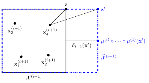
Figure 5: Extended domain for multi-output chains.

Since $\widetilde{\mathcal{X}}^{(i+1)}$ is a hyperrectangle and $\mu^{(i)}_{T}\circ\cdots\circ\mu^{(1)}({\mathbf{x}}^{\prime})\in\widetilde{\mathcal{X}}^{(i+1)}$, it follows from (113) that

$$\widetilde{\Gamma}_{T}^{(i+1)}({\mathbf{x}}^{\prime}) =O\big{(}(\delta^{\prime}_{i+1})^{\nu}\big{)}$$ (174)

$$=O\Bigg{(}\Big{(}\max\Big{\{}L^{i}T^{-1/d},iB\cdot\max_{j\in[i]}L^{i-j}\widetilde{\Gamma}_{T}^{(j)}({\mathbf{x}}^{\prime})\Big{\}}\Big{)}^{\nu}\Bigg{)}.$$ (175)

By 4, we also have

$$\widetilde{\Gamma}_{T}^{(1)}({\mathbf{x}}^{\prime})=\|\Gamma_{T}^{(1)}({\mathbf{x}}^{\prime})\|_{2}^{1/2}=\sigma_{T}^{(1)}({\mathbf{x}}^{\prime})=O\big{(}(\delta_{T})^{\nu})=O(T^{-\nu/d}).$$ (176)

This recursive relation is exactly the same as that of chains in (147), showing 4 extends to multi-output chains.

For the two more restrictive cases, 2, with the same posterior standard deviation upper bound as 1, implies that the results in Section D.2 also extend to multi-output chains.

∎

D.4 Non-Adaptive Sampling Method for Feed-Forward Networks

For feed-forward networks of scalar-valued functions, let $\mu^{(i,j)}_{T}$ denote the posterior mean of $f^{(i,j)}$ computed using (3) based on $\{(\mathbf{x}^{(i)}_{s},\mathbf{x}^{(i+1,j)}_{s})\}_{s=1}^{T}$. The composite posterior mean of $g({\mathbf{x}})$ with feed-forward network structure is

$$\mu_{T}^{g}({\mathbf{x}})=\mu^{(m,1)}_{T}(\mathbf{z}^{(m)})$$ (177)

with

$$\mathbf{z}^{(1)} ={\mathbf{x}},$$ (178)

$$\mathbf{z}^{(i+1,j)} =\mu^{(i,j)}_{T}(\mathbf{z}^{(i)}) \text{ for }i\in[m-1],j\in[d_{i+1}],$$ (179)

$$\mathbf{z}^{(i+1)} =\mu^{(i)}_{T}(\mathbf{z}^{(i)})=[\mathbf{z}^{(i+1,1)},\dots,\mathbf{z}^{(i+1,d_{i})}] \text{ for }i\in[m-1].$$ (180)

Aussiming each $\mathcal{X}^{(i)}$ is a hyperrectangle of dimension $d_{i}$, the following theorem provides the upper bound on simple regret of Algorithm 2 using (177) for feed-forward networks.

Theorem 8 (Non-adaptive sampling method for feed-forward networks).

Under the setup of Section 2, given $B=\Theta(L)$, $k=k_{\text{Mat\'{e}rn}}$, and a feed-forward network $g=f^{(m)}\circ f^{(m-1)}\circ\cdots\circ f^{(1)}$ with $f^{(i)}({\mathbf{z}})=[f^{(i,j)}({\mathbf{z}})]_{j=1}^{d_{i+1}}$, $f^{(i,j)}\in\mathcal{H}_{k}(B)\cap\mathcal{F}(L)$, and $\mathcal{X}^{(i)}$ being a hyperrectangle for each $i\in[m],j\in[d_{i+1}]$,

• when $\nu\leq 1$, Algorithm 2 achieves

  $$r^{\ast}_{T}={\widetilde{O}}(\sqrt{D_{2,m}}BL^{m-1}T^{-\nu^{m}/d});$$ (181)

• when $\nu>1$, Algorithm 2 achieves

  $$r^{\ast}_{T}={\widetilde{O}}\Big{(}\max\Big{\{}(D_{2,m})^{\nu/2}BL^{(m-1)\nu}T^{-\nu/d},{\widetilde{D}}_{2,m}^{\nu}B^{1+\nu+\nu^{2}+\cdots+\nu^{m-2}}L^{\nu^{m-1}}T^{-\nu^{2}/d}\Big{\}}\Big{)},$$ (182)

where $D_{2,m}=\prod_{i=2}^{m}d_{i}$ and ${\widetilde{D}}_{2,m}^{\nu}=\prod_{i=2}^{m}(d_{i})^{\nu^{m+1-i}/2}$.

Proof.

With $\mu^{(i)}_{T}(\cdot)=[\mu^{(i,j)}_{T}(\cdot)]_{j=1}^{d_{i+1}}$, we have

$$\|f^{(i)}({\mathbf{z}})-\mu^{(i)}_{T}({\mathbf{z}})\|_{2} =\sqrt{\sum_{j=1}^{d_{i+1}}\big{(}f^{(i,j)}({\mathbf{z}})-\mu^{(i,j)}_{T}({\mathbf{z}})\big{)}^{2}}$$ (183)

$$\leq\sqrt{\sum_{j=1}^{d_{i+1}}\big{(}B\sigma^{(i,j)}_{T}({\mathbf{z}})\big{)}^{2}}$$ (184)

$$=\sqrt{d_{i+1}}B\sigma^{(i,1)}_{T}({\mathbf{z}}),$$ (185)

where we use the confidence bounds and the fact that $\sigma^{(i,j)}_{T}({\mathbf{z}})=\sigma^{(i,1)}_{T}({\mathbf{z}})$ by the symmetry of our setup.

Since each $f^{(i,j)}$ is Lipschitz continuous with parameter $L$, we have that $f^{(i)}$ is Lipschitz continuous with parameter $\sqrt{d_{i+1}}L$, and $f^{(m)}\circ\cdots\circ f^{(i)}$ is Lipschitz continuous with parameter $\sqrt{D_{i+1,m+1}}L^{m-i+1}$, where $D_{i,j}=\prod_{s=i}^{j}d_{s}$ and $d_{m+1}=1$. Then, defining ${\widetilde{\sigma}}_{T}^{(i,1)}({\mathbf{x}})=(\sigma^{(i,1)}_{T}\circ\mu^{(i-1)}_{T}\circ\cdots\circ\mu^{(1)}_{T})({\mathbf{x}})$, we can follow (126)–(132) to obtain

$$g({\mathbf{x}})={} (f^{(m)}\circ f^{(m-1)}\circ\cdots\circ f^{(2)})\big{(}f^{(1)}({\mathbf{x}})\big{)}$$ (186)

$$\leq{} (f^{(m)}\circ f^{(m-1)}\circ\cdots\circ f^{(2)})\big{(}\mu^{(1)}_{T}({\mathbf{x}})\big{)}+\sqrt{D_{3,m+1}}L^{m-1}\|f^{(1)}({\mathbf{x}})-\mu^{(1)}_{T}({\mathbf{x}})\|_{2}$$ (187)

$$={} (f^{(m)}\circ f^{(m-1)}\circ\cdots\circ f^{(2)})\big{(}\mu^{(1)}_{T}({\mathbf{x}})\big{)}+\sqrt{D_{2,m+1}}L^{m-1}B\sigma^{(1,1)}_{T}({\mathbf{x}})$$ (188)

$$\leq{} (f^{(m)}\circ f^{(m-1)}\circ\cdots\circ f^{(3)})\big{(}(\mu^{(2)}_{T}\circ\mu^{(1)}_{T})({\mathbf{x}})\big{)}+\sqrt{D_{3,m+1}}L^{m-2}B\sigma^{(2,1)}_{T}\big{(}\mu^{(1)}_{T}({\mathbf{x}})\big{)}$$

$$+\sqrt{D_{2,m+1}}L^{m-1}B\sigma^{(1,1)}_{T}({\mathbf{x}})$$ (189)

$$\leq{} (\mu^{(m)}_{T}\circ\mu^{(m-1)}_{T}\circ\cdots\circ\mu^{(1)}_{T})({\mathbf{x}})+B\sigma^{(m,1)}\big{(}(\mu^{(m-1)}_{T}\circ\cdots\circ\mu^{(1)}_{T})({\mathbf{x}})\big{)}$$

$$+LB\sigma^{(m-1)}\big{(}(\mu^{(m-2)}_{T}\circ\cdots\circ\mu^{(1)}_{T})({\mathbf{x}})\big{)}+\cdots+\sqrt{D_{2,m+1}}L^{m-1}B\sigma^{(1,1)}_{T}({\mathbf{x}})$$ (190)

$$\leq{} (\mu^{(m)}_{T}\circ\mu^{(m-1)}_{T}\circ\cdots\circ\mu^{(1)}_{T})({\mathbf{x}})+B\sum_{i=1}^{m}\sqrt{D_{i+1,m+1}}L^{m-i}{\widetilde{\sigma}}_{T}^{(i,1)}({\mathbf{x}}).$$ (191)

Hence, we have

$$r^{\ast}_{T} =g({\mathbf{x}}^{\ast})-g({\mathbf{x}}^{\ast}_{T})\leq 2B\sum_{i=1}^{m}\sqrt{D_{i+1,m}}L^{m-i}\max\{{\widetilde{\sigma}}^{(i,1)}_{T}({\mathbf{x}}^{\ast}),{\widetilde{\sigma}}^{(i,1)}_{T}({\mathbf{x}}^{\ast}_{T})\}.$$ (192)

It remains to upper bound $\max\{{\widetilde{\sigma}}^{(i,1)}_{T}({\mathbf{x}}^{\ast}),{\widetilde{\sigma}}^{(i,1)}_{T}({\mathbf{x}}^{\ast}_{T})\}$ for $i\in[m]$. Firstly, by 5, we have

$${\widetilde{\sigma}}^{(1,1)}_{T}({\mathbf{x}})=\sigma^{(1,1)}_{T}({\mathbf{x}})=O\big{(}(\delta_{T})^{\nu}\big{)}=O(T^{-\nu/d}).$$ (193)

We now represent the upper bound on ${\widetilde{\sigma}}^{(i+1,1)}_{T}(\cdot)$ in terms of $\{{\widetilde{\sigma}}^{(j,1)}_{T}(\cdot):j\in[i]\}$ for $i\in[m-1]$. For all ${\mathbf{x}}\in\mathcal{X}$, the distance between $\mu^{(i)}_{T}\circ\cdots\circ\mu^{(1)}_{T}({\mathbf{x}})$ and its closest point in $\mathcal{X}^{(i+1)}$ is

$$\delta_{i+1}({\mathbf{x}}) =\min_{{\mathbf{z}}\in\mathcal{X}^{(i+1)}}|(\mu^{(i)}_{T}\circ\cdots\circ\mu^{(1)}_{T})({\mathbf{x}})-{\mathbf{z}}|$$ (194)

$$\leq|(\mu^{(i)}_{T}\circ\cdots\circ\mu^{(1)}_{T})({\mathbf{x}})-f^{(i)}\circ\cdots\circ f^{(1)}({\mathbf{x}})|$$ (195)

$$\leq B\sum_{j=1}^{i}\sqrt{D_{j+1,i+1}}L^{i-j}{\widetilde{\sigma}}^{(j,1)}_{T}({\mathbf{x}}),$$ (196)

where the last step follows from (191). Then, the distance between $(\mu^{(i)}_{T}\circ\cdots\circ\mu^{(1)}_{T})({\mathbf{x}})$ and its closest point in $\mathcal{X}^{(i+1)}_{T}$ is

$$\delta^{\prime}_{i+1}({\mathbf{x}}) =\min_{s\in[T]}|(\mu^{(i)}_{T}\circ\cdots\circ\mu^{(1)}_{T})({\mathbf{x}})-\mathbf{x}^{(i+1)}_{s}|$$ (197)

$$\leq\delta^{(i+1)}_{T}+\delta_{i+1}({\mathbf{x}})$$ (198)

$$\leq O(\sqrt{D_{2,i+1}}L^{i}T^{-1/d})+B\sum_{j=1}^{i}\sqrt{D_{j+1,i+1}}L^{i-j}{\widetilde{\sigma}}^{(j,1)}_{T}({\mathbf{x}})$$ (199)

$$=O\Big{(}\max\Big{\{}\sqrt{D_{2,i+1}}L^{i}T^{-1/d},iB\cdot\max_{j\in[i]}\sqrt{D_{j+1,i+1}}L^{i-j}{\widetilde{\sigma}}^{(j,1)}_{T}({\mathbf{x}})\Big{\}}\Big{)},$$ (200)

where (198) applies the triangle inequality, and (199) uses (123) and (196).

Now, for each ${\mathbf{x}}^{\prime}\in\{{\mathbf{x}}^{\ast},{\mathbf{x}}^{\ast}_{T}\}$, we extend $\mathcal{X}^{(i+1)}$ to $\widetilde{\mathcal{X}}^{(i+1)}$, the smallest hyperrectangle that covers $(\mu^{(i)}_{T}\circ\cdots\circ\mu^{(1)}_{T})({\mathbf{x}}^{\prime})$ and $\mathcal{X}^{(i+1)}$. Then, the fill distance of the extended domain with regard to $\mathcal{X}^{(i+1)}_{T}$ is

$$\delta^{\prime}_{i+1}=O\Big{(}\max\Big{\{}\sqrt{D_{2,i+1}}L^{i}T^{-1/d},iB\cdot\max_{j\in[i]}\sqrt{D_{j+1,i+1}}L^{i-j}{\widetilde{\sigma}}^{(j,1)}_{T}({\mathbf{x}}^{\prime})\Big{\}}\Big{)},$$ (201)

and by 5, we have

$${\widetilde{\sigma}}^{(i+1,1)}_{T}({\mathbf{x}}^{\prime})=O\big{(}(\delta^{\prime}_{i+1})^{\nu}\big{)}=O\Bigg{(}\Big{(}\max\Big{\{}\sqrt{D_{2,i+1}}L^{i}T^{-1/d},iB\cdot\max_{j\in[i]}\sqrt{D_{j+1,i+1}}L^{i-j}{\widetilde{\sigma}}^{(j,1)}_{T}({\mathbf{x}}^{\prime})\Big{\}}\Big{)}^{\nu}\Bigg{)}.$$ (202)

We now consider two cases;

The case that $\nu\leq 1$: Recalling the assumption $B=\Theta(L)$, and using the fact that ${\widetilde{O}}(L^{c\nu})$ is equivalent to $O\big{(}(L^{c\nu}{\rm poly}(c\log L))\big{)}$ for fixed $\nu$, it follows from (193) and (202) that when $\nu\leq 1$, we have

$${\widetilde{\sigma}}_{T}^{(2,1)}({\mathbf{x}}^{\prime}) =O\Big{(}\max\Big{\{}(d_{2})^{\nu/2}L^{\nu}T^{-\nu/d},(d_{2})^{\nu/2}B^{\nu}T^{-\nu^{2}/d}\Big{\}}\Big{)}=O\big{(}(d_{2})^{\nu/2}L^{\nu}T^{-\nu^{2}/d}\big{)},$$ (203)

$${\widetilde{\sigma}}^{(3,1)}_{T}({\mathbf{x}}^{\prime}) =O\Big{(}\max\Big{\{}(D_{2,3})^{\nu/2}L^{2\nu}T^{-\nu/d},2^{\nu}(D_{2,3})^{\nu/2}B^{\nu}L^{\nu}T^{-\nu^{2}/d},2^{\nu}(d_{3})^{\nu/2}B^{\nu}(d_{2})^{\nu^{2}/2}L^{\nu^{2}}T^{-\nu^{3}/d}\Big{\}}\Big{)}$$

$$=O\big{(}2^{\nu}(D_{2,3})^{\nu/2}B^{\nu}L^{\nu}T^{-\nu^{3}/d}\big{)}={\widetilde{O}}\big{(}(D_{2,3})^{\nu/2}B^{\nu}L^{\nu}T^{-\nu^{3}/d}\big{)},$$ (204)

$$\mathmakebox[width("{}={}")][c]{\vdots}$$

$${\widetilde{\sigma}}^{(i,1)}_{T}({\mathbf{x}}^{\prime}) ={\widetilde{O}}\big{(}(i-1)^{\nu}(D_{2,i})^{\nu/2}B^{\nu}L^{(i-2)\nu}T^{-\nu^{i}/d}\big{)}={\widetilde{O}}\big{(}(D_{2,i})^{\nu/2}B^{\nu}L^{(i-2)\nu}T^{-\nu^{i}/d}\big{)},$$ (205)

and the simple regret is

$$r^{\ast}_{T} \leq 2B\sum_{i=1}^{m}\sqrt{D_{i+1,m}}L^{m-i}\max\{{\widetilde{\sigma}}^{(i,1)}_{T}({\mathbf{x}}^{\ast}),{\widetilde{\sigma}}^{(i,1)}_{T}({\mathbf{x}}^{\ast}_{T})\}$$ (206)

$$={\widetilde{O}}(\sqrt{D_{2,m}}BL^{m-1}T^{-\nu^{m}/d}).$$ (207)

The case that $\nu>1$: With $B=\Theta(L)$, and using the property of ${\widetilde{O}}(\cdot)$ similar to the first case, it follows from (193) and (202) that when $\nu>1$, we have

$${\widetilde{\sigma}}_{T}^{(2,1)}({\mathbf{x}}^{\prime}) =O\Big{(}\max\Big{\{}(d_{2})^{\nu/2}L^{\nu}T^{-\nu/d},(d_{2})^{\nu/2}B^{\nu}T^{-\nu^{2}/d}\Big{\}}\Big{)}=O((d_{2})^{\nu/2}L^{\nu}T^{-\nu/d}),$$ (208)

$${\widetilde{\sigma}}^{(3,1)}_{T}({\mathbf{x}}^{\prime}) =O\Big{(}\max\Big{\{}(D_{2,3})^{\nu/2}L^{2\nu}T^{-\nu/d},(d_{3})^{\nu/2}B^{\nu}(d_{2})^{\nu^{2}/2}L^{\nu^{2}}T^{-\nu^{2}/d}\Big{\}}\Big{)}$$

$$=O\big{(}2^{\nu}(d_{3})^{\nu/2}(d_{2})^{\nu^{2}/2}B^{\nu}L^{\nu^{2}}T^{-\nu/d}\big{)}={\widetilde{O}}\big{(}(d_{3})^{\nu/2}(d_{2})^{\nu^{2}/2}B^{\nu}L^{\nu^{2}}T^{-\nu/d}\big{)},$$ (209)

$$\mathmakebox[width("{}={}")][c]{\vdots}$$

$${\widetilde{\sigma}}^{(i,1)}_{T}({\mathbf{x}}^{\prime}) ={\widetilde{O}}\Big{(}\max\Big{\{}(D_{2,i})^{\nu/2}L^{(i-1)\nu}T^{-\nu/d},(i-1)^{\nu}(d_{i})^{\nu/2}(d_{i-1})^{\nu^{2}/2}\cdots(d_{2})^{\nu^{i-1}/2}B^{\nu+\cdots+\nu^{i-2}}L^{\nu^{i-1}}T^{-\nu^{2}/d}\Big{\}}\Big{)}$$

$$={\widetilde{O}}\Big{(}\max\Big{\{}(D_{2,i})^{\nu/2}L^{(i-1)\nu}T^{-\nu/d},(d_{i})^{\nu/2}(d_{i-1})^{\nu^{2}/2}\cdots(d_{2})^{\nu^{i-1}/2}B^{\nu+\cdots+\nu^{i-2}}L^{\nu^{i-1}}T^{-\nu^{2}/d}\Big{\}}\Big{)},$$ (210)

and the simple regret is

$$r^{\ast}_{T} \leq 2B\sum_{i=1}^{m}\sqrt{D_{i+1,m}}L^{m-i}\max\{{\widetilde{\sigma}}^{(i,1)}_{T}({\mathbf{x}}^{\ast}),{\widetilde{\sigma}}^{(i,1)}_{T}({\mathbf{x}}^{\ast}_{T})\}$$ (211)

$$={\widetilde{O}}\Big{(}\max\Big{\{}(D_{2,m})^{\nu/2}BL^{(m-1)\nu}T^{-\nu/d},{\widetilde{D}}_{2,m}^{\nu}B^{1+\nu+\nu^{2}+\cdots+\nu^{m-2}}L^{\nu^{m-1}}T^{-\nu^{2}/d}\Big{\}}\Big{)},$$ (212)

where ${\widetilde{D}}_{2,m}^{\nu}=\prod_{i=2}^{m}(d_{i})^{\nu^{m+1-i}/2}$. ∎

Next, we recall the following two restrictive cases introduced in the main body:

• Case 1: We additionally assume that $(\mu^{(i)}_{T}\circ\cdots\circ\mu^{(1)}_{T})({\mathbf{x}}^{\ast})\in\mathcal{X}^{(i+1)}$ and $(\mu^{(i)}_{T}\circ\cdots\circ\mu^{(1)}_{T})({\mathbf{x}}^{\ast}_{T})\in\mathcal{X}^{(i+1)}$ for $i\in[m-1]$.

• Case 2: We additionally assume that all the $\mathcal{X}^{(i)}$’s are known. Defining

  $$\widetilde{\mu}^{(i)}_{T}({\mathbf{z}}) =\operatorname*{arg\,min}_{{\mathbf{z}}^{\prime}\in\mathcal{X}^{(i+1)}}|\mu^{(i)}_{T}({\mathbf{z}})-{\mathbf{z}}^{\prime}|,$$ (213)

  we let the algorithm return

  $${\mathbf{x}}^{\ast}_{T}=\operatorname*{arg\,max}_{{\mathbf{x}}\in\mathcal{X}}(\widetilde{\mu}^{(m)}_{T}\circ\cdots\circ\widetilde{\mu}^{(1)}_{T})({\mathbf{x}}).$$ (214)

Similarly to chains and multi-output chains, in either case, it follows that

$$r^{\ast}_{T}\leq 2B\sum_{i=1}^{m}\sqrt{D_{i+1,m}}L^{m-i}\max\{{\widetilde{\sigma}}^{(i,1)}_{T}({\mathbf{x}}^{\ast}),{\widetilde{\sigma}}^{(i,1)}_{T}({\mathbf{x}}^{\ast}_{T})\}=O\Big{(}B\sum_{i=1}^{m}\sqrt{D_{i+1,m}}L^{m-i}{\mkern 1.25mu\overline{\mkern-1.25mu\sigma\mkern-0.25mu}\mkern 0.25mu}_{T}^{(i,1)}\Big{)}.$$ (215)

Moreover, by 3, we can further upper bound this by

$$r^{\ast}_{T}\leq O\Big{(}B\sum_{i=1}^{m}\sqrt{D_{i+1,m}}L^{m-i}{\mkern 1.25mu\overline{\mkern-1.25mu\sigma\mkern-0.25mu}\mkern 0.25mu}_{T}^{(i,1)}\Big{)}=\begin{cases}O(\sqrt{D_{2,m}}BL^{m-1}T^{-\nu/d})&\text{ when $\nu\leq 1$,}\\ O\big{(}(D_{2,m})^{\nu/2}BL^{(m-1)\nu}T^{-\nu/d}\big{)}&\text{ when $\nu>1$.}\end{cases}$$ (216)

Appendix E Lower Bound on Simple Regret (Proof of 5)

Recall the high-level intuition behind our lower bound outlined in Section 5: We use the idea from (Bull, 2011) of having a small bump that is difficult to locate, but unlike (Bull, 2011), we exploit Lipschitz functions at the intermediate layers to “amplify” that bump (which means the original bump can have a much narrower width for a given RKHS norm).

We first show that, for fixed $\epsilon>0$, we can construct a base function ${\mkern 1.25mu\overline{\mkern-1.25mug\mkern-0.25mu}\mkern 0.25mu}$ with height $2\epsilon$ and support radius $w=\Theta\big{(}(\frac{\epsilon}{BL^{m-1}})^{1/\nu}\big{)}$ for each network structure.

E.1 Hard Function for Chains

To construct a base function with chain structure, we define the following two scalar-valued functions.

Considering the “bump” function $h({\mathbf{x}})=\exp\big{(}\frac{-1}{1-\|{\mathbf{x}}\|_{2}^{2}}\big{)}\mathds{1}\{\|{\mathbf{x}}\|_{2}<1\}$, for some $\epsilon_{1}>0$ and width $w>0$, we define (Bull, 2011)

$${\widetilde{h}}({\mathbf{x}},\epsilon_{1},w) =\frac{2\epsilon_{1}}{h(\mathbf{0})}h\Big{(}\frac{{\mathbf{x}}}{w}\Big{)},$$ (217)

which is a scaled bump function with height $2\epsilon_{1}$ and compact support $\{{\mathbf{x}}\in\mathcal{X}:\|{\mathbf{x}}\|_{2}<w\}$.

For a fixed $u>0$ and ${\widetilde{L}}=\sqrt{2}B/\sqrt{k(0)-k(2u)}$, where $k$ is the Matérn kernel on ${\mathbb{R}}$ with smoothness $\nu$ and $k(|x-x^{\prime}|)=k(x,x^{\prime})$, we define

$${\widetilde{g}}_{k}(\cdot) =\frac{{\widetilde{L}}}{2}\big{(}k(\cdot,u)-k(\cdot,-u)\big{)}.$$ (218)

Theorem 9 (Hard function for chains).

For the Matérn kernel $k$ with smoothness $\nu\geq 1$, sufficiently small $\epsilon>0$, and sufficiently large $B$, there exists $\epsilon_{1}>0,L=\Theta(B),c=\Theta(1),w=\Theta\big{(}(\frac{\epsilon}{B(cL)^{m-1}})^{1/\nu}\big{)},$ and $u>0$ such that ${\mkern 1.25mu\overline{\mkern-1.25mug\mkern-0.25mu}\mkern 0.25mu}:={\mkern 1.25mu\overline{\mkern-1.25muf\mkern-0.25mu}\mkern 0.25mu}^{(m)}\circ{\mkern 1.25mu\overline{\mkern-1.25muf\mkern-0.25mu}\mkern 0.25mu}^{(m-1)}\circ\cdots\circ{\mkern 1.25mu\overline{\mkern-1.25muf\mkern-0.25mu}\mkern 0.25mu}^{(1)}$ with ${\mkern 1.25mu\overline{\mkern-1.25muf\mkern-0.25mu}\mkern 0.25mu}^{(1)}(\cdot)={\widetilde{h}}(\cdot,\epsilon_{1},w)$ and ${\mkern 1.25mu\overline{\mkern-1.25muf\mkern-0.25mu}\mkern 0.25mu}^{(s)}(\cdot)={\widetilde{g}}_{k}(\cdot)$ for $s\in[2,m]$ has the following properties:

• ${\mkern 1.25mu\overline{\mkern-1.25muf\mkern-0.25mu}\mkern 0.25mu}^{(i)}\in\mathcal{H}_{k}(B)\cap\mathcal{F}(L)$ for each $i\in[m]$,

• $\max_{{\mathbf{x}}}{\mkern 1.25mu\overline{\mkern-1.25mug\mkern-0.25mu}\mkern 0.25mu}({\mathbf{x}})=2\epsilon$,

• ${\mkern 1.25mu\overline{\mkern-1.25mug\mkern-0.25mu}\mkern 0.25mu}({\mathbf{x}})>0$ when $\|{\mathbf{x}}\|_{2}<w$ , and ${\mkern 1.25mu\overline{\mkern-1.25mug\mkern-0.25mu}\mkern 0.25mu}({\mathbf{x}})=0$ otherwise.

Proof.

For $k$ being the Matérn kernel with smoothness $\nu$, recalling that

$${\widetilde{h}}({\mathbf{x}},\epsilon_{1},w) =\frac{2\epsilon_{1}}{h(\mathbf{0})}h\Big{(}\frac{{\mathbf{x}}}{w}\Big{)}$$ (219)

with $h$ being the bump function, (Bull, 2011, Section A.2) has shown that for some constant $C_{1}$,

$$\|{\widetilde{h}}\|_{k}\leq C_{1}\frac{2\epsilon_{1}}{h(\mathbf{0})}\Big{(}\frac{1}{w}\Big{)}^{\nu}\|h\|_{k}.$$ (220)

Hence, we have $\|{\widetilde{h}}\|_{k}\leq B$ when $w=\big{(}\frac{2C_{1}\|h\|_{k}\epsilon_{1}}{h(\mathbf{0})B}\big{)}^{1/\nu}$. When $\frac{\epsilon_{1}}{B}$ is sufficiently small, the diameter of the support satisfies $2w\ll 1$. Since the bump function is infinitely differentiable, ${\widetilde{h}}$ is Lipschitz continuous with some constant $L^{\prime}=\Theta(\frac{\epsilon_{1}}{w})$, and our assumption of $\nu\geq 1$ further implies $L^{\prime}=O(B)$.

Recall that for a fixed $u>0$ and the Matérn kernel $k$ on a one-dimension domain, we define

$${\widetilde{g}}_{k}(\cdot) =\frac{{\widetilde{L}}}{2}\big{(}k(\cdot,u)-k(\cdot,-u)\big{)}$$ (221)

with ${\widetilde{L}}=\frac{\sqrt{2}B}{\sqrt{k(0)-k(2u)}}$. Applying (1) with ${\widetilde{g}}_{k}$ replacing both $f$ and $f^{\prime}$, we have

$$\|{\widetilde{g}}_{k}\|_{k}=\frac{{\widetilde{L}}}{2}\sqrt{k(u,u)+2k(u,-u)+k(-u,-u)}=\frac{{\widetilde{L}}}{2}\sqrt{2k(0)-2k(2u)}=B,$$ (222)

where $k(d_{{\mathbf{x}},{\mathbf{x}}^{\prime}})=k({\mathbf{x}},{\mathbf{x}}^{\prime})$ with $d_{{\mathbf{x}},{\mathbf{x}}^{\prime}}=\|{\mathbf{x}}-{\mathbf{x}}^{\prime}\|_{2}$.

We choose the two constants $u>{\widetilde{u}}>0$ to satisfy the following:

1. $k(d_{{\mathbf{x}},{\mathbf{x}}^{\prime}})$ is non-increasing when $d_{{\mathbf{x}},{\mathbf{x}}^{\prime}}\in[u-{\widetilde{u}},u+{\widetilde{u}}]$.

2. $k(u-{\widetilde{u}})-k(u+{\widetilde{u}})\geq\frac{2}{{\widetilde{L}}}=\frac{\sqrt{2}\sqrt{k(0)-k(2u)}}{B}$.

3. Defining $r_{\max}=\sup_{z\in(0,{\widetilde{u}}]}\frac{k(u-z)-k(u+z)}{2z}$ and $r_{\min}=\inf_{z\in(0,{\widetilde{u}}]}\frac{k(u-z)-k(u+z)}{2z}$, it holds that $r_{\max}=\Theta(1)$ and $r_{\min}=\Theta(1)$.

Whenever $k(d_{{\mathbf{x}},{\mathbf{x}}^{\prime}})$ is continuous and non-increasing in $d_{{\mathbf{x}},{\mathbf{x}}^{\prime}}$ on ${\mathbb{R}}^{+}$ (e.g., the Matérn kernel), condition 1 is satisfied. This condition guarantees that $k(\cdot,u)$ is non-decreasing on $[0,{\widetilde{u}}]$, and $k(\cdot,-u)$ is non-increasing on $[0,{\widetilde{u}}]$, which together implies that ${\widetilde{g}}_{k}$ is non-decreasing on $[0,{\widetilde{u}}]$. Under condition 1, condition 2 is satisfied as long as $B$ is sufficiently large, and it implies that ${\widetilde{g}}_{k}({\widetilde{u}})\geq 1$. Examples of ${\widetilde{g}}_{k}$ for $k=k_{\text{Mat\'{e}rn}}$ are given in Figure 6.

Let $L=\max\{L^{\prime},\sup_{z\in(0,{\widetilde{u}}]}\frac{{\widetilde{g}}_{k}(z)}{z}\}=\max\{L^{\prime},r_{\max}{\widetilde{L}}\}$ and $\alpha=\inf_{z\in(0,{\widetilde{u}}]}\frac{{\widetilde{g}}_{k}(z)}{zL}=\frac{r_{\min}{\widetilde{L}}}{L}$. Then, it holds for all $z\in(0,{\widetilde{u}}]$ that

$$1<\alpha L\leq\frac{{\widetilde{g}}_{k}(z)}{z}\leq L.$$ (223)

Clearly $\alpha$ cannot exceed $1$, and moreover, condition 3 above along with $L^{\prime}=O(B)$ implies that $\alpha=\min\big{\{}r_{\min}\sqrt{\frac{2}{k(0)-k(2u)}}\frac{B}{L^{\prime}},\frac{r_{\min}}{r_{\max}}\big{\}}=\Theta(1)$.

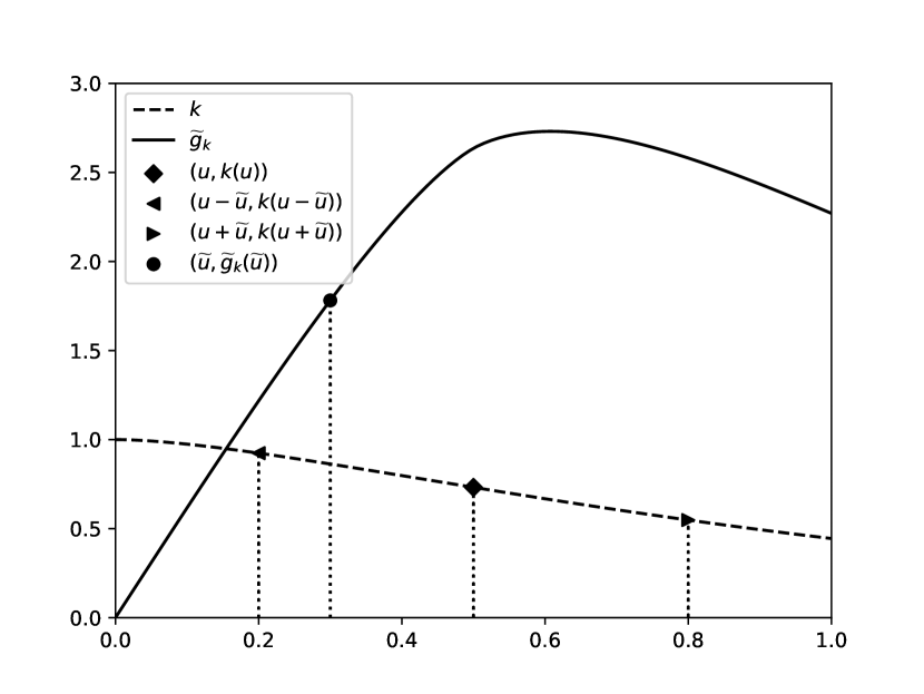
$\nu=1$

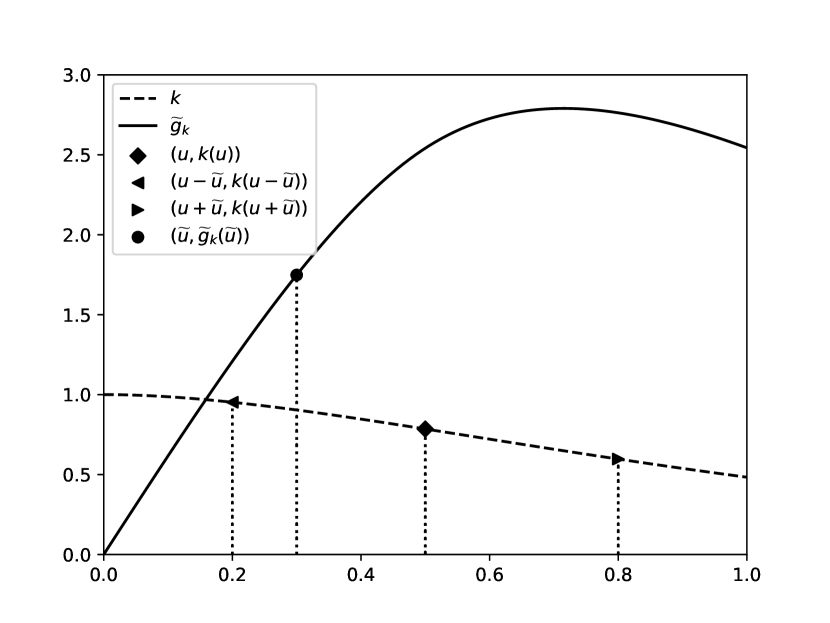
$\nu=3/2$

$\nu=2$

Figure 6: $k=k_{\text{Mat\'{e}rn}}$ with lengthscale $l=1$ and smoothness $\nu$, and ${\widetilde{g}}_{k}$ with $B=5$, $u=0.5$, and ${\widetilde{u}}=0.3$.

Defining ${\mkern 1.25mu\overline{\mkern-1.25mug\mkern-0.25mu}\mkern 0.25mu}_{i}={\mkern 1.25mu\overline{\mkern-1.25muf\mkern-0.25mu}\mkern 0.25mu}^{(i)}\circ{\mkern 1.25mu\overline{\mkern-1.25muf\mkern-0.25mu}\mkern 0.25mu}^{(i-1)}\circ\dots\circ{\mkern 1.25mu\overline{\mkern-1.25muf\mkern-0.25mu}\mkern 0.25mu}^{(1)}$, we denote the height of ${\mkern 1.25mu\overline{\mkern-1.25mug\mkern-0.25mu}\mkern 0.25mu}_{i}$ by $h_{i}=\max_{\mathbf{x}}{\mkern 1.25mu\overline{\mkern-1.25mug\mkern-0.25mu}\mkern 0.25mu}_{i}({\mathbf{x}})$. If $h_{i-1}\leq{\widetilde{u}}$, (223) implies

$$h_{i-1}<\alpha Lh_{i-1}\leq h_{i}\leq Lh_{i-1}.$$ (224)

Then, for a given $\epsilon\in(0,{\widetilde{g}}_{k}({\widetilde{u}})]$, where condition 2 implies ${\widetilde{g}}_{k}({\widetilde{u}})\geq 1$, we choose $\epsilon_{1}$ to satisfy

$$({\mkern 1.25mu\overline{\mkern-1.25muf\mkern-0.25mu}\mkern 0.25mu}^{(m)}\circ\cdots\circ{\mkern 1.25mu\overline{\mkern-1.25muf\mkern-0.25mu}\mkern 0.25mu}^{(2)})(2\epsilon_{1})=({\widetilde{g}}_{k}\circ\cdots\circ{\widetilde{g}}_{k})(2\epsilon_{1})=2\epsilon.$$ (225)

By $h_{1}=2\epsilon_{1}$ and (224), this choice of $\epsilon_{1}$ must also satisfy

$$2(\alpha L)^{m-1}\epsilon_{1}=(\alpha L)^{m-1}h_{1}\leq h_{m}=2\epsilon\leq L^{m-1}h_{1}=2L^{m-1}\epsilon_{1},$$ (226)

implying (via (223)) that

$$\frac{\epsilon}{L^{m-1}}\leq\epsilon_{1}\leq\frac{\epsilon}{(\alpha L)^{m-1}}<\epsilon.$$ (227)

Since ${\widetilde{h}}$ has a compact support with radius $w$ and ${\widetilde{g}}(0)=0$, ${\mkern 1.25mu\overline{\mkern-1.25mug\mkern-0.25mu}\mkern 0.25mu}$ also has a compact support with radius

$$w=\Theta\bigg{(}\Big{(}\frac{\epsilon_{1}}{B}\Big{)}^{1/\nu}\bigg{)}=\Theta\bigg{(}\Big{(}\frac{\epsilon}{B(cL)^{m-1}}\Big{)}^{1/\nu}\bigg{)},$$ (228)

for some constant $c=\Theta(1)$.

Lastly, (223) implies ${\widetilde{g}}_{k}$ on $[0,{\widetilde{u}}]$ is a member of $\mathcal{F}(L)$, and $L\geq L^{\prime}$ guarantees ${\widetilde{h}}\in\mathcal{F}(L)$. ∎

E.2 Hard Function for Multi-Output Chains

In this section, we consider the operator-valued Matérn kernel $\Gamma^{(i)}({\mathbf{x}},{\mathbf{x}}^{\prime})=k^{(i)}({\mathbf{x}},{\mathbf{x}}^{\prime}){\mathbf{I}}^{(i+1)}$, where $k^{(i)}$ is the scalar-valued Matérn kernel on ${\mathbb{R}}^{d_{i}}$ and ${\mathbf{I}}^{(i+1)}$ is the identity matrix of size $d_{i+1}$. Then, for a fixed ${\mathbf{u}}^{(i)}\in{\mathbb{R}}^{d_{i}}$ and ${\widetilde{L}}^{(i)}=\sqrt{2}B/\sqrt{k^{(i)}(0)-k^{(i)}(2\|{\mathbf{u}}^{(i)}\|_{2})}$ where $k^{(i)}(\|{\mathbf{x}}-{\mathbf{x}}^{\prime}\|_{2})=k^{(i)}({\mathbf{x}},{\mathbf{x}}^{\prime})$, we define

$${\widetilde{g}}^{(i)}(\cdot) =\frac{{\widetilde{L}}^{(i)}}{2}\big{(}\Gamma^{(i)}(\cdot,{\mathbf{u}}^{(i)})-\Gamma^{(i)}(\cdot,-{\mathbf{u}}^{(i)})\big{)}.$$ (229)

Theorem 10 (Hard function for multi-output chains).

Let ${\mathbf{I}}^{(i)}$ denote the identity matrix of size $d_{i}$, let ${\mathbf{e}}^{(i)}_{1}$ denote the first column of ${\mathbf{I}}^{(i)}$, and let $k^{(i)}$ denote the scalar-valued Matérn kernel on ${\mathbb{R}}^{d_{i}}$ with smoothness $\nu\geq 1$. For $\Gamma^{(i)}({\mathbf{x}},{\mathbf{x}}^{\prime})=k^{(i)}({\mathbf{x}},{\mathbf{x}}^{\prime}){\mathbf{I}}^{(i+1)}$, sufficiently small $\epsilon>0$, and sufficiently large $B$, there exists $\epsilon_{1}>0,L=\Theta(B),c=\Theta(1),w=\Theta\big{(}(\frac{\epsilon}{B(cL)^{m-1}})^{1/\nu}\big{)},$ and $u\in{\mathbb{R}}$ such that ${\mkern 1.25mu\overline{\mkern-1.25mug\mkern-0.25mu}\mkern 0.25mu}:={\mkern 1.25mu\overline{\mkern-1.25muf\mkern-0.25mu}\mkern 0.25mu}^{(m)}\circ{\mkern 1.25mu\overline{\mkern-1.25muf\mkern-0.25mu}\mkern 0.25mu}^{(m-1)}\circ\cdots\circ{\mkern 1.25mu\overline{\mkern-1.25muf\mkern-0.25mu}\mkern 0.25mu}^{(1)}$ with ${\mkern 1.25mu\overline{\mkern-1.25muf\mkern-0.25mu}\mkern 0.25mu}^{(1)}(\cdot)={\widetilde{h}}(\cdot,\epsilon_{1},w){\mathbf{e}}_{1}^{(2)}$ and ${\mkern 1.25mu\overline{\mkern-1.25muf\mkern-0.25mu}\mkern 0.25mu}^{(s)}(\cdot)={\widetilde{g}}^{(s)}(\cdot){\mathbf{e}}_{1}^{(s+1)}$ with ${\mathbf{u}}^{(s)}=u{\mathbf{e}}_{1}^{(s)}$ for $s\in[2,m]$ has the following properties:

• ${\mkern 1.25mu\overline{\mkern-1.25muf\mkern-0.25mu}\mkern 0.25mu}^{(i)}\in\mathcal{H}_{\Gamma^{(i)}}(B)\cap\mathcal{F}(L)$ for each $i\in[m]$,

• $\max_{{\mathbf{x}}}{\mkern 1.25mu\overline{\mkern-1.25mug\mkern-0.25mu}\mkern 0.25mu}({\mathbf{x}})=2\epsilon$,

• ${\mkern 1.25mu\overline{\mkern-1.25mug\mkern-0.25mu}\mkern 0.25mu}({\mathbf{x}})>0$ when $\|{\mathbf{x}}\|_{2}<w$ , and ${\mkern 1.25mu\overline{\mkern-1.25mug\mkern-0.25mu}\mkern 0.25mu}({\mathbf{x}})=0$ otherwise.

Proof.

The rough idea is to reduce to the case of regular chains by only making use of a single coordinate throughout the network. We leave open the question as to whether the lower bound can be improved by utilizing all coordinates.

With ${\mathbf{I}}$ denoting the identity matrix of size $d_{2}$ and ${\mathbf{e}}_{1}$ denoting the first column of ${\mathbf{I}}$, we aim to show that ${\mkern 1.25mu\overline{\mkern-1.25muf\mkern-0.25mu}\mkern 0.25mu}^{(1)}\in\mathcal{H}_{\Gamma^{(1)}}(B)$ by showing that if $\Gamma(\cdot,\cdot)=k(\cdot,\cdot){\mathbf{I}}\in{\mathbb{R}}^{d_{2}\times d_{2}}$ and ${\widetilde{h}}\in\mathcal{H}_{k}(B)$ for some scalar-valued kernel $k$ and some constant $B$, then the function ${\widetilde{h}}^{\prime}(\cdot)={\widetilde{h}}(\cdot){\mathbf{e}}_{1}$ satisfies ${\widetilde{h}}^{\prime}\in\mathcal{H}_{\Gamma}(B)$. Since ${\widetilde{h}}\in\mathcal{H}_{k}(B)$, there exists a sequence $\{(a_{i},{\mathbf{x}}_{i})\}_{i=1}^{\infty}$ such that ${\widetilde{h}}(\cdot)=\sum_{i=1}^{\infty}a_{i}k(\cdot,{\mathbf{x}}_{i})$. Then, using the definition of RKHS norm for vector-valued functions in (2), we have

$$\|{\widetilde{h}}^{\prime}\|_{\Gamma}^{2} =\lim_{n\to\infty}\Big{\|}\sum_{i=1}^{n}a_{i}k(\cdot,{\mathbf{x}}_{i}){\mathbf{e}}_{1}\Big{\|}_{\Gamma}^{2}$$ (230)

$$=\lim_{n\to\infty}\Big{\|}\sum_{i=1}^{n}a_{i}\Gamma(\cdot,{\mathbf{x}}_{i}){\mathbf{e}}_{1}\Big{\|}_{\Gamma}^{2}$$ (231)

$$=\sum_{i,j=1}^{\infty}\langle\Gamma({\mathbf{x}}_{i},{\mathbf{x}}_{j})(a_{i}{\mathbf{e}}_{1}),a_{j}{\mathbf{e}}_{1}\rangle$$ (232)

$$=\sum_{i,j=1}^{\infty}a_{i}a_{j}k({\mathbf{x}}_{i},{\mathbf{x}}_{j})$$ (233)

$$=\|{\widetilde{h}}\|_{k}^{2}$$ (234)

$$\leq B^{2},$$ (235)

and therefore ${\widetilde{h}}^{\prime}\in\mathcal{H}_{\Gamma}(B)$. Next, for $i\in[2,m]$, with ${\mathbf{u}}^{(i)}=u{\mathbf{e}}_{1}^{(i)}$ we have

$$\|{\mkern 1.25mu\overline{\mkern-1.25muf\mkern-0.25mu}\mkern 0.25mu}^{(i)}\|_{\Gamma} =\frac{{\widetilde{L}}^{(i)}}{2}\sqrt{\langle\Gamma^{(i)}({\mathbf{u}}^{(i)},{\mathbf{u}}^{(i)}){\mathbf{e}}_{1},{\mathbf{e}}_{1}\rangle-2\langle\Gamma^{(i)}({\mathbf{u}}^{(i)},-{\mathbf{u}}^{(i)}){\mathbf{e}}_{1},{\mathbf{e}}_{1}\rangle+\langle\Gamma^{(i)}(-{\mathbf{u}}^{(i)},-{\mathbf{u}}^{(i)}){\mathbf{e}}_{1},{\mathbf{e}}_{1}\rangle}$$ (236)

$$=\frac{{\widetilde{L}}^{(i)}}{2}\sqrt{k^{(i)}({\mathbf{u}}^{(i)},{\mathbf{u}}^{(i)})-2k^{(i)}({\mathbf{u}}^{(i)},-{\mathbf{u}}^{(i)})+k^{(i)}(-{\mathbf{u}}^{(i)},-{\mathbf{u}}^{(i)})}$$ (237)

$$=\frac{{\widetilde{L}}^{(i)}}{2}\sqrt{2k^{(i)}(0)-2k^{(i)}(2u)}$$ (238)

$$=B.$$ (239)

Since ${\widetilde{h}}\in\mathcal{F}(L^{\prime})$ for some $L^{\prime}>1$, we also have ${\widetilde{h}}^{\prime}\in\mathcal{F}(L^{\prime})$.

We reuse the choice of $u$ and ${\widetilde{u}}$ in the previous case. Then, for any $z\in{\mathbb{R}}$, with ${\mathbf{z}}^{(i)}=z{\mathbf{e}}_{1}^{(i)}$ and ${\mathbf{u}}^{(i)}=u{\mathbf{e}}_{1}^{(i)}$, we have

$${\mkern 1.25mu\overline{\mkern-1.25muf\mkern-0.25mu}\mkern 0.25mu}^{(i)}({\mathbf{z}}) ={\widetilde{g}}^{(i)}({\mathbf{z}}^{(i)},{\mathbf{u}}^{(i)}){\mathbf{e}}_{1}^{(i+1)}$$ (240)

$$=\frac{{\widetilde{L}}^{(i)}}{2}\big{(}\Gamma^{(i)}({\mathbf{z}}^{(i)},{\mathbf{u}}^{(i)})-\Gamma^{(i)}({\mathbf{z}}^{(i)},-{\mathbf{u}}^{(i)})\big{)}{\mathbf{e}}_{1}^{(i+1)}$$ (241)

$$=\frac{{\widetilde{L}}^{(i)}}{2}\big{(}k^{(i)}({\mathbf{z}}^{(i)},{\mathbf{u}}^{(i)})-k^{(i)}({\mathbf{z}}^{(i)},-{\mathbf{u}}^{(i)})\big{)}{\mathbf{e}}_{1}^{(i+1)}$$ (242)

$$=\frac{{\widetilde{L}}^{(i)}}{2}\big{(}k(\|{\mathbf{z}}^{(i)}-{\mathbf{u}}^{(i)}\|)-k(\|{\mathbf{z}}^{(i)}+{\mathbf{u}}^{(i)}\|)\big{)}{\mathbf{e}}_{1}^{(i+1)}$$ (243)

$$=\frac{{\widetilde{L}}}{2}\big{(}k(|z-u|)-k(|z+u|)\big{)}{\mathbf{e}}_{1}^{(i+1)}$$ (244)

$$={\widetilde{g}}_{k}(z){\mathbf{e}}_{1}^{(i+1)},$$ (245)

where ${\widetilde{g}}_{k}(\cdot)$ depending on $u$ is defined in (218). Hence, as illustrated in Figure 7, for any input ${\mathbf{x}}\in[0,1]^{d}$ of ${\mkern 1.25mu\overline{\mkern-1.25mug\mkern-0.25mu}\mkern 0.25mu}$, we have

$$\mathbf{x}^{(2,1)} ={\widetilde{h}}({\mathbf{x}}),$$ (246)

$$\mathbf{x}^{(2,j)} =0 \text{ for }j\geq 2,$$ (247)

$$\mathbf{x}^{(i+1,1)} ={\widetilde{g}}_{k}(\mathbf{x}^{(i,1)}) \text{ for }i\geq 2,$$ (248)

$$\mathbf{x}^{(i+1,j)} =0 \text{ for }i\geq 2\text{ and }j\geq 2.$$ (249)

Figure 7: Illustration of ${\mkern 1.25mu\overline{\mkern-1.25mug\mkern-0.25mu}\mkern 0.25mu}$ for multi-output chain.

By a similar argument to the case of single-output chains, there exists $L\geq L^{\prime}$ and $\alpha=\Theta(1)$ such that for all $z\in[0,{\widetilde{u}}]$,

$$1<\alpha L\leq\frac{{\widetilde{g}}_{k}(z)}{z}\leq L.$$ (250)

For $\epsilon\leq{\widetilde{g}}_{k}({\widetilde{u}})$, we choose $\epsilon_{1}$ to satisfy

$$({\mkern 1.25mu\overline{\mkern-1.25muf\mkern-0.25mu}\mkern 0.25mu}^{(m)}\circ{\mkern 1.25mu\overline{\mkern-1.25muf\mkern-0.25mu}\mkern 0.25mu}^{(m-1)}\circ\cdots\circ{\mkern 1.25mu\overline{\mkern-1.25muf\mkern-0.25mu}\mkern 0.25mu}^{(2)})(2\epsilon_{1}{\mathbf{e}}_{1}^{(2)})=({\widetilde{g}}_{k}\circ\cdots\circ{\widetilde{g}}_{k})(2\epsilon_{1})=2\epsilon,$$ (251)

and ${\mkern 1.25mu\overline{\mkern-1.25mug\mkern-0.25mu}\mkern 0.25mu}$ has a compact support with radius

$$w=\Theta\Bigg{(}\Big{(}\frac{\epsilon_{1}}{B}\Big{)}^{1/\nu}\Bigg{)}=\Theta\Bigg{(}\Big{(}\frac{\epsilon}{B(cL)^{m-1}}\Big{)}^{1/\nu}\Bigg{)},$$ (252)

for some constant $c=\Theta(1)$.

Lastly, since $L\geq L^{\prime}$, we immediately deduce that ${\mkern 1.25mu\overline{\mkern-1.25muf\mkern-0.25mu}\mkern 0.25mu}^{(i)}\in\mathcal{F}(L)$ on its domain for each $i\in[m]$. ∎

E.3 Hard Function for Feed-Forward Networks

For a fixed ${\mathbf{u}}^{(i)}\in{\mathbb{R}}^{d_{i}}$ and ${\widetilde{L}}^{(i)}=\sqrt{2}B/\sqrt{k^{(i)}(0)-k^{(i)}(2\|{\mathbf{u}}^{(i)}\|_{2})}$, where $k^{(i)}(\|{\mathbf{x}}-{\mathbf{x}}^{\prime}\|_{2})=k^{(i)}({\mathbf{x}},{\mathbf{x}}^{\prime})$, we define

$${\widetilde{g}}_{k}^{(i)}(\cdot) =\frac{{\widetilde{L}}^{(i)}}{2}\big{(}k^{(i)}(\cdot,{\mathbf{u}}^{(i)})-k^{(i)}(\cdot,-{\mathbf{u}}^{(i)})\big{)}.$$ (253)

Theorem 11 (Hard function for feed-forward networks).

Let ${\mathbf{e}}_{1}^{(i)}$ denote the first column of identity matrix of size $d_{i}$. For the Matérn kernel $k$ with smoothness $\nu\geq 1$, sufficiently small $\epsilon>0$, and sufficiently large $B$, there exists $\epsilon_{1}>0,L=\Theta(B),c=\Theta(1),w=\Theta\big{(}(\frac{\epsilon}{B(cL)^{m-1}})^{1/\nu}\big{)},$ and $u>0$ such that ${\mkern 1.25mu\overline{\mkern-1.25mug\mkern-0.25mu}\mkern 0.25mu}:={\mkern 1.25mu\overline{\mkern-1.25muf\mkern-0.25mu}\mkern 0.25mu}^{(m)}\circ{\mkern 1.25mu\overline{\mkern-1.25muf\mkern-0.25mu}\mkern 0.25mu}^{(m-1)}\circ\cdots\circ{\mkern 1.25mu\overline{\mkern-1.25muf\mkern-0.25mu}\mkern 0.25mu}^{(1)}$ with ${\mkern 1.25mu\overline{\mkern-1.25muf\mkern-0.25mu}\mkern 0.25mu}^{(i)}(\cdot)=[{\mkern 1.25mu\overline{\mkern-1.25muf\mkern-0.25mu}\mkern 0.25mu}^{(i,j)}(\cdot)]_{j=1}^{d_{i+1}}$ for $i\in[m]$, ${\mkern 1.25mu\overline{\mkern-1.25muf\mkern-0.25mu}\mkern 0.25mu}^{(1,1)}(\cdot)={\widetilde{h}}(\cdot,\epsilon_{1},w)$, ${\mkern 1.25mu\overline{\mkern-1.25muf\mkern-0.25mu}\mkern 0.25mu}^{(s,1)}(\cdot)={\widetilde{g}}_{k}^{(s)}(\cdot)$ with ${\mathbf{u}}^{(s)}=u{\mathbf{e}}_{1}^{(s)}$, and ${\mkern 1.25mu\overline{\mkern-1.25muf\mkern-0.25mu}\mkern 0.25mu}^{(s,r)}(\cdot)=0$ for $s\in[2,m]$ and $r\neq 1$ has the following properties:

• ${\mkern 1.25mu\overline{\mkern-1.25muf\mkern-0.25mu}\mkern 0.25mu}^{(i,j)}\in\mathcal{H}_{k}(B)\cap\mathcal{F}(L)$ for each $i\in[m],j\in[d_{i+1}]$;

• $\max_{{\mathbf{x}}}{\mkern 1.25mu\overline{\mkern-1.25mug\mkern-0.25mu}\mkern 0.25mu}({\mathbf{x}})=2\epsilon$;

• ${\mkern 1.25mu\overline{\mkern-1.25mug\mkern-0.25mu}\mkern 0.25mu}({\mathbf{x}})>0$ when $\|{\mathbf{x}}\|_{2}<w$ , and ${\mkern 1.25mu\overline{\mkern-1.25mug\mkern-0.25mu}\mkern 0.25mu}({\mathbf{x}})=0$ otherwise.

Proof.

We adopt a similar general approach to the case of chains and multi-output chains, but with some different details.

As noted in our analysis of chains, we have ${\widetilde{h}}\in\mathcal{H}_{k}(B)$ and ${\widetilde{h}}\in\mathcal{F}(L^{\prime})$ for some constant $L^{\prime}>1$, and we also have

$$\|{\widetilde{g}}^{(i)}_{k}\|_{k} =\frac{{\widetilde{L}}^{(i)}}{2}\sqrt{k^{(i)}({\mathbf{u}}^{(i)},{\mathbf{u}}^{(i)})-2k^{(i)}({\mathbf{u}}^{(i)},-{\mathbf{u}}^{(i)})+k^{(i)}(-{\mathbf{u}}^{(i)},-{\mathbf{u}}^{(i)})}$$ (254)

$$=\frac{{\widetilde{L}}^{(i)}}{2}\sqrt{2k^{(i)}(0)-2k^{(i)}(2\|{\mathbf{u}}^{(i)}\|_{2})}$$ (255)

$$=B.$$ (256)

Reusing the choice of $u$ and ${\widetilde{u}}$ in the case of chains, with ${\mathbf{z}}^{(i)}=z{\mathbf{e}}_{1}^{(i)}$ and ${\mathbf{u}}^{(i)}=u{\mathbf{e}}_{1}^{(i)}$, we have

$${\widetilde{g}}^{(i)}_{k}({\mathbf{z}}^{(i)}) =\frac{{\widetilde{L}}^{(i)}}{2}\big{(}k^{(i)}({\mathbf{z}}^{(i)},{\mathbf{u}}^{(i)})-k^{(i)}({\mathbf{z}}^{(i)},-{\mathbf{u}}^{(i)})\big{)}$$ (257)

$$=\frac{{\widetilde{L}}^{(i)}}{2}\big{(}k^{(i)}(\|{\mathbf{z}}^{(i)}-{\mathbf{u}}^{(i)}\|_{2})-k^{(i)}(\|{\mathbf{z}}^{(i)}+{\mathbf{u}}^{(i)}\|_{2})\big{)}$$ (258)

$$=\frac{{\widetilde{L}}^{(i)}}{2}\big{(}k^{(i)}(|z-u|)-k^{(i)}(|z+u|)\big{)}$$ (259)

$$={\widetilde{g}}_{k}(z)$$ (260)

Hence, as illustrated in Figure 8, for any input ${\mathbf{x}}\in[0,1]^{d}$ of ${\mkern 1.25mu\overline{\mkern-1.25mug\mkern-0.25mu}\mkern 0.25mu}$, we have

$$\mathbf{x}^{(2,1)} ={\widetilde{h}}({\mathbf{x}}),$$ (261)

$$\mathbf{x}^{(2,j)} =0 \text{ for }j\geq 2,$$ (262)

$$\mathbf{x}^{(i+1,1)} ={\widetilde{g}}_{k}(\mathbf{x}^{(i,1)}) \text{ for }i\geq 2,$$ (263)

$$\mathbf{x}^{(i+1,j)} =0 \text{ for }i\geq 2\text{ and }j\geq 2.$$ (264)

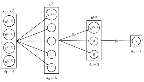
Figure 8: Illustration of ${\mkern 1.25mu\overline{\mkern-1.25mug\mkern-0.25mu}\mkern 0.25mu}$ for feed-forward network.

By a similar argument to the previous cases, there exists $L\geq L^{\prime}$ and $\alpha=\Theta(1)$ such that for all $z\in[0,{\widetilde{u}}]$,

$$1<\alpha L\leq\frac{{\widetilde{g}}_{k}(z)}{z}\leq L.$$ (265)

For $\epsilon\leq{\widetilde{g}}_{k}({\widetilde{u}})$, we choose $\epsilon_{1}$ satisfying

$$({\mkern 1.25mu\overline{\mkern-1.25muf\mkern-0.25mu}\mkern 0.25mu}^{(m)}\circ{\mkern 1.25mu\overline{\mkern-1.25muf\mkern-0.25mu}\mkern 0.25mu}^{(m-1)}\circ\cdots\circ{\mkern 1.25mu\overline{\mkern-1.25muf\mkern-0.25mu}\mkern 0.25mu}^{(2)})(2\epsilon_{1}{\mathbf{e}}_{1}^{(2)})=({\widetilde{g}}_{k}\circ\cdots\circ{\widetilde{g}}_{k})(2\epsilon_{1})=2\epsilon,$$ (266)

and ${\mkern 1.25mu\overline{\mkern-1.25mug\mkern-0.25mu}\mkern 0.25mu}$ has a compact support with radius

$$w=\Theta\Bigg{(}\Big{(}\frac{\epsilon_{1}}{B}\Big{)}^{1/\nu}\Bigg{)}=\Theta\Bigg{(}\Big{(}\frac{\epsilon}{B(cL)^{m-1}}\Big{)}^{1/\nu}\Bigg{)},$$ (267)

for some constant $c=\Theta(1)$.

Lastly, due to $L\geq L^{\prime}$, ${\mkern 1.25mu\overline{\mkern-1.25muf\mkern-0.25mu}\mkern 0.25mu}^{(i,j)}\in\mathcal{F}(L)$ on its domain for each $i\in[m],j\in[d_{i+1}]$. ∎

E.4 Lower Bound on Simple Regret

With the preceding “hard functions” established, the final step is to essentially follow that of (Bull, 2011). We provide the details for completeness.

By splitting the domain $\mathcal{X}=[0,1]^{d}$ into a grid of dimension $d$ with spacing $2w$, we construct $M=(\lfloor\frac{1}{2w}\rfloor)^{d}$ functions with disjoint supports by shifting the origin of ${\mkern 1.25mu\overline{\mkern-1.25mug\mkern-0.25mu}\mkern 0.25mu}$ to the center of each cell and cropping the shifted function into $[0,1]^{d}$, which is denoted by $\mathcal{G}=\{g_{1},\dots,g_{M}\}$. For $g$ sampled uniformly from $\mathcal{G}$, we first show that the expected simple regret ${\mathbb{E}}[r_{T}^{\ast}]$ of an arbitrary algorithm is lower bounded, then there must exist a function in $\mathcal{G}$ that has the same lower bound.

Now, we prove 5, which is restated as follows. See 5

Proof.

Since the theorem concerns worst-case RKHS functions, it suffices to establish the same result when the function $g$ is drawn uniformly from the hard subset $\mathcal{G}$ introduced above. Given that $g$ is random, Yao’s minimax principle implies that it suffices to consider deterministic algorithms.

For any given deterministic algorithm, let $\mathcal{X}^{\prime}_{T}=\{{\mathbf{x}}^{\prime}_{1},{\mathbf{x}}^{\prime}_{2},\cdots,{\mathbf{x}}^{\prime}_{T}\}$ be the set of points that it would sample if the function were zero everywhere. We observe that if $g=g_{i}$ for some $g_{i}$ satisfying $g({\mathbf{x}}^{\prime}_{1})=g({\mathbf{x}}^{\prime}_{2})=\dotsc=g({\mathbf{x}}^{\prime}_{T})=0$ (i.e., the bump in $g_{i}$ does not cover any of the points in $\mathcal{X}^{\prime}_{T}$), then the algorithm will precisely sample ${\mathbf{x}}^{\prime}_{1},{\mathbf{x}}^{\prime}_{2},\cdots,{\mathbf{x}}^{\prime}_{T}$. Moreover, if there are multiple such functions $g_{i}$, then the final returned point ${\mathbf{x}}_{T}^{*}$ can only be below $2\epsilon$ (i.e., the bump height) for at most one of those functions, since their supports are disjoint by construction.

Now suppose that $T\leq\frac{M}{2}-1$, where $M$ is the number of functions in $\mathcal{G}$. This means that regardless of the values ${\mathbf{x}}^{\prime}_{1},{\mathbf{x}}^{\prime}_{2},\cdots,{\mathbf{x}}^{\prime}_{T}$, there are at least $\frac{M}{2}+1$ functions in $\mathcal{G}$ such that the sampled values are all zero. Hence, there are at least $\frac{M}{2}$ functions where a simple regret of at least $2\epsilon$ is incurred, meaning that the average simple regret is at least $\epsilon$.

With this result in place, 5 immediately follows by substituting $M=\Theta\big{(}(1/w)^{d}\big{)}$ and $w=\Theta\big{(}(\frac{\epsilon}{B(cL)^{m-1}})^{1/\nu}\big{)}$. ∎

Appendix F Lower Bound on Cumulative Regret (Proof of 6)

In this section, we prove 6, which is restated as follows. See 6

Proof.

By rearranging 5, we have $\epsilon=\Omega(B(cL)^{m-1}T^{-\nu/d})$, which implies that the lower bound on cumulative regret is

$${\mathbb{E}}[R_{T}]=\Omega(\epsilon T)=\Omega(B(cL)^{m-1}T^{1-\nu/d}).$$ (268)

However, this lower bound is loose when $d<\nu$. 5 implies that to have simple regret at most $\epsilon=\Theta(1)$ requires $T=\Omega\big{(}(B(cL)^{m-1})^{d/\nu}\big{)}$. When $T=\Theta\big{(}(B(cL)^{m-1})^{d/\nu}\big{)}$, we have ${\mathbb{E}}[r^{\ast}_{T}]=\Omega(1)$ and ${\mathbb{E}}[R_{T}]=\Omega\big{(}(B(cL)^{m-1})^{d/\nu}\big{)}$. Since cumulative regret is always non-decreasing in $T$, when $T=\Omega\big{(}(B(cL)^{m-1})^{d/\nu}\big{)}$, we also have ${\mathbb{E}}[R_{T}]=\Omega\big{(}(B(cL)^{m-1})^{d/\nu}\big{)}$.

For $T=o\big{(}(B(cL)^{m-1})^{d/\nu}\big{)}$ (which is equivalent to $T=o(B(cL)^{m-1}T^{1-\nu/d})$), we show by contradiction that ${\mathbb{E}}[R_{T}]=\Omega(T)$. Suppose on the contrary that there exists an algorithm guaranteeing ${\mathbb{E}}[R_{T}]=o(T)$ when $T=T_{0}$ for some $T_{0}=o\big{(}(B(cL)^{m-1})^{d/\nu}\big{)}$. Then, by repeatedly selecting the best point among the first $T_{0}$ time steps, the algorithm attains ${\mathbb{E}}[R_{T}]=o\big{(}(B(cL)^{m-1})^{d/\nu}\big{)}$ when $T=\Theta\big{(}(B(cL)^{m-1})^{d/\nu}\big{)}$, which contradicts the lower bound for $T=\Omega\big{(}(B(cL)^{m-1})^{d/\nu}\big{)}$.

Hence, 6 follows by combining the two cases.

∎

Appendix G Summary of Regret Bounds

A detailed summary of our regret bounds for the Matérn kernel is given in Table 2.

Algorithm-Independent Cumulative Regret Lower Bound
Chains/Multi-Output Chains/Feed-Forward Networks	$\begin{cases}\Omega\big{(}\min\{T,B(cL)^{m-1}T^{1-\nu/d}\}\big{)}&\text{ when }d>\nu\geq 1,\\ \Omega\big{(}\min\{T,(B(cL)^{m-1})^{d/\nu}\}\big{)}&\text{ when }d\leq\nu.\end{cases}$
Algorithmic Cumulative Regret Upper Bound
(If Conjecture of (Vakili, 2022) Holds)
Chains	$\begin{cases}O(2^{m}BL^{m-1}T^{1-\nu/d})&\text{ when }d>\nu,\\ {\widetilde{O}}(2^{m}BL^{m-1})&\text{ when }d\leq\nu.\end{cases}$
Multi-Output Chains	$\begin{cases}O(5^{m}BL^{m-1}T^{1-\nu/d_{\max}})&\text{ when }d_{\max}>\nu,\\ {\widetilde{O}}(5^{m}BL^{m-1})&\text{ when }d_{\max}\leq\nu.\end{cases}$
Feed-Forward Networks	$\begin{cases}O(2^{m}\sqrt{D_{2,m}}BL^{m-1}T^{1-\nu/d_{\max}})&\text{ when }d_{\max}>\nu,\\ {\widetilde{O}}(2^{m}\sqrt{D_{2,m}}BL^{m-1})&\text{ when }d_{\max}\leq\nu.\end{cases}$
Algorithm-Independent Simple Regret Lower Bound
Chains/Multi-Output Chains/Feed-Forward Networks	$\Omega(B(cL)^{m-1}T^{-\nu/d})$      when $\nu\geq 1.$
Algorithmic Simple Regret Upper Bound
Chains/Multi-Output Chains	$\begin{cases}{\widetilde{O}}(BL^{m-1}T^{-\nu^{m}/d})&\text{when $\nu\leq 1$,}\\ {\widetilde{O}}(B^{1+\nu+\nu^{2}+\nu^{m-2}}L^{\nu^{m-1}}T^{-\nu/d})&\text{when $\nu>1$.}\end{cases}$
Chains/Multi-Output Chains (Restrictive Cases)	$\begin{cases}O(BL^{m-1}T^{-\nu/d})&\text{ when $\nu\leq 1$,}\\ O(BL^{(m-1)\nu}T^{-\nu/d})&\text{ when $\nu>1$.}\end{cases}$
Feed-Forward Networ ks	$\begin{cases}{\widetilde{O}}(\sqrt{D_{2,m}}BL^{m-1}T^{-\nu^{m}/d})&\text{ when $\nu\leq 1$,}\\ {\widetilde{O}}({\widetilde{D}}_{2,m}^{\nu}B^{1+\nu+\nu^{2}+\nu^{m-2}}L^{\nu^{m-1}}T^{-\nu/d})&\text{ when $\nu>1$.}\end{cases}$
Feed-Forward Networks (Restrictive Cases)	$\begin{cases}O(\sqrt{D_{2,m}}BL^{m-1}T^{-\nu/d})&\text{ when $\nu\leq 1$,}\\ O\big{(}(D_{2,m})^{\nu/2}BL^{(m-1)\nu}T^{-\nu/d}\big{)}&\text{ when $\nu>1$.}\end{cases}$

Table 2: Summary of regret bounds for the Matérn kernel. (The algorithmic simple regret upper bounds are valid when the domain of each layer is a hyperrectangle.) $T$ denotes the time horizon; $m$ denotes the number of layers; $B$ denotes the RKHS norm upper bound of each layer; $L$ denotes the Lipschitz constant upper bound of each layer; $\nu$ denotes the smoothness of the Matérn kernel; $d$ denotes the domain dimension of $g$; $d_{\max}=\max_{i\in[m]}d_{i}$ denotes the maximum dimension among all the $m$ layers; $D_{2,m}=\prod_{i=2}^{m}d_{i}$ denotes the product of the dimensions from the second to the last layer; ${\widetilde{D}}_{2,m}^{\nu}=\prod_{i=2}^{m}(d_{i})^{\nu^{m+1-i}/2}$. The lower bounds hold for some $c=\Theta(1)$.

Appendix H Comparison to (Kusakawa et al., 2021)

In this section, we compare our work to (Kusakawa et al., 2021), which proposed two confidence bound based algorithms cascade UCB (cUCB) and optimistic improvement (OI) under the noise-free setting. Both algorithms utilize a novel posterior standard deviation defined using the Lipschitz constant.

Problem Setup.

• In each layer, (Kusakawa et al., 2021) assumes the entries in the same layer are mutually independent, which is equivalent to our feed-forward network structure.

• Different from our assumption of $f^{(i,j)}\in\mathcal{H}_{k}(B)\cap\mathcal{F}(L,\|\cdot\|_{2})$ for each $i\in[m]$ and $j\in[d_{i+1}]$, where the Lipschitz continuity is with respect to $\|\cdot\|_{2}$, (Kusakawa et al., 2021) assumes $f^{(i,j)}\in\mathcal{H}_{k}(B)\cap\mathcal{F}(L_{f},\|\cdot\|_{1})$, where the Lipschitz continuity is with respect to $\|\cdot\|_{1}$. Therefore, for a fixed scalar-valued function $f^{(i,j)}\in\mathcal{F}(L,\|\cdot\|_{2})\cap\mathcal{F}(L_{f},\|\cdot\|_{1})$ with the smallest possible $L$ and $L_{f}$, it is satisfied that $L_{f}\leq L\leq\sqrt{d_{i}}L_{f}$.

• (Kusakawa et al., 2021) has an additional assumption that $\sigma^{(i,j)}_{t}\in\mathcal{F}(L_{\sigma},\|\cdot\|_{1})$ for all $t\geq 1$ for some constant $L_{\sigma}$. The constant $L_{\sigma}$ is not used in the algorithms, and only appears in the regret bounds.

Regret Bounds.

• cUCB achieves cumulative regret $R_{T}=O\big{(}B(BL_{\sigma}+L_{f})^{m-1}D_{2,m}(\sum_{i=2}^{m}d_{i})\sqrt{T\gamma_{T}}\big{)}$, with a significantly larger $T$-independent factor than that in $R_{T}=O(2^{m}BL^{m-1}\sqrt{D_{2,m}T\gamma_{T}})$ of our GPN-UCB (Algorithm 1).

• OI achieves simple regret $r^{\ast}_{T}=O\big{(}m^{m^{2}+m+\frac{1}{2}}B^{m+1}L_{f}^{m^{3}}(BL_{\sigma}+L_{f})^{3m^{3}}(D_{2,m})^{2m^{2}}(\sum_{i=2}^{m}d_{i})^{m^{2}+1}T^{-\frac{\nu}{2\nu+d}}\big{)}$ for the Matérn kernel with smoothness $\nu$. When $\nu\leq 1$, our non-adaptive sampling (Algorithm 2) achieves $r^{\ast}_{T}={\widetilde{O}}(\sqrt{D_{2,m}}BL^{m-1}T^{-\nu^{m}/d})$, which has a significantly smaller $T$-independent factor. When $\nu>1$, our Algorithm 2 achieves $r^{\ast}_{T}={\widetilde{O}}({\widetilde{D}}_{2,m}^{\nu}B^{1+\nu+\nu^{2}+\nu^{m-2}}L^{\nu^{m-1}}T^{-\nu/d})$, which has a smaller $T$-dependent factor. The $T$-independent factors are more difficult to compare, though ours certainly become preferable under the more restrictive scenarios discussed leading up to (25).

Generality. (Kusakawa et al., 2021) allows additional (multi-dimensional) input independent of previous layers for each layer. GPN-UCB and non-adaptive sampling can also be adapted to accept additional input. Let $\widehat{\mathcal{X}}^{(i)}\subset{\mathbb{R}}^{{\widehat{d}}_{i}}$ denote the domain of the additional input of $f^{(i)}$, and let $\widehat{{\mathbf{x}}}_{[i:j]}=[\widehat{{\mathbf{x}}}^{(i)},\dots,\widehat{{\mathbf{x}}}^{(j)}]$ denote the concatenation of the addition inputs from $f^{(i)}$ to $f^{(j)}$.

• For GPN-UCB (Algorithm 1), we simply modify the upper confidence bound to be

  $$\mathrm{UCB}_{t}({\mathbf{x}},\widehat{{\mathbf{x}}}) =\max_{{\mathbf{z}}\in\Delta^{(m)}_{t}({\mathbf{x}},\widehat{{\mathbf{x}}}_{[2:m-1]})}\overline{\mathrm{UCB}}^{(m,1)}_{t}([{\mathbf{z}},\widehat{{\mathbf{x}}}^{(m)}]),$$ (269)

  where

  $$\Delta^{(1)}_{t}({\mathbf{x}})= \{{\mathbf{x}}\},$$ (270)

  $$\Delta^{(i+1,j)}_{t}({\mathbf{x}},\widehat{{\mathbf{x}}}_{[2:i]})= \Bigg{[}\min_{{\mathbf{z}}\in\Delta^{(i)}_{t}({\mathbf{x}},\widehat{{\mathbf{x}}}_{[2:i-1]})}\overline{\mathrm{LCB}}^{(i,j)}_{t}([{\mathbf{z}},\widehat{{\mathbf{x}}}^{(i)}]),\max_{{\mathbf{z}}\in\Delta^{(i)}_{t}({\mathbf{x}},\widehat{{\mathbf{x}}}_{[2:i-1]})}\overline{\mathrm{UCB}}^{(i,j)}_{t}([{\mathbf{z}},\widehat{{\mathbf{x}}}^{(i)}])\Bigg{]}$$

  $$\hskip 180.83276pt\text{ for }i\in[m-1],j\in[d_{i+1}],$$ (271)

  $$\Delta^{(i)}_{t}({\mathbf{x}},\widehat{{\mathbf{x}}}_{[2:i-1]})= \Delta^{(i,1)}_{t}({\mathbf{x}},\widehat{{\mathbf{x}}}_{[2:i-1]})\times\cdots\times\Delta^{(i,d_{i})}_{t}({\mathbf{x}},\widehat{{\mathbf{x}}}_{[2:i-1]})$$

  $$\hskip 241.11035pt\text{ for }i\in[m].$$ (272)

  The cumulative regret upper bound will remain the same, since $\mathrm{diam}\big{(}\Delta^{(i)}_{t}({\mathbf{x}},\widehat{{\mathbf{x}}}_{[2:i-1]})\big{)}$ remains the same.

• For non-adaptive sampling (Algorithm 2), with ${\widehat{d}}=d+\sum_{i=2}^{m}{\widehat{d}}_{i}$, we choose $\{{\mathbf{x}}_{s},\widehat{{\mathbf{x}}}^{(2)}_{s},\dots,\widehat{{\mathbf{x}}}^{(m)}_{s}\}_{s=1}^{T}$ such that

  $$\max_{[{\mathbf{x}},\widehat{{\mathbf{x}}}^{(2)},\dots,\widehat{{\mathbf{x}}}^{(m)}]\in\mathcal{X}\times\widehat{\mathcal{X}}^{(2)}\times\cdots\times\widehat{\mathcal{X}}^{(m)}}\min_{s\in[T]}\|[{\mathbf{x}},\widehat{{\mathbf{x}}}^{(2)},\dots,\widehat{{\mathbf{x}}}^{(m)}]-[{\mathbf{x}}_{s},\widehat{{\mathbf{x}}}^{(2)}_{s},\dots,\widehat{{\mathbf{x}}}^{(m)}_{s}]\|_{2}=O(T^{-1/{\widehat{d}}}).$$ (273)

  Then, modify the composite mean to be

  $$\mu_{T}^{g}({\mathbf{x}},\widehat{{\mathbf{x}}})=\mu^{(m,1)}_{T}([\mathbf{z}^{(m)},\widehat{{\mathbf{x}}}^{(m)}])$$ (274)

  with

  $$\mathbf{z}^{(1)} ={\mathbf{x}},$$ (275)

  $$\mathbf{z}^{(i+1,j)} =\mu^{(i,j)}_{T}([\mathbf{z}^{(i)},\widehat{{\mathbf{x}}}^{(i)}]) \text{ for }i\in[m-1],j\in[d_{i+1}],$$ (276)

  $$\mathbf{z}^{(i+1)} =\mu^{(i)}_{T}([\mathbf{z}^{(i)},\widehat{{\mathbf{x}}}^{(i)}])=[\mathbf{z}^{(i+1,1)},\dots,\mathbf{z}^{(i+1,d_{i})}] \text{ for }i\in[m-1].$$ (277)

  Then, the only change in simple regret upper bound is that $d$ is replaced by ${\widehat{d}}$.

References

- Astudillo & Frazier (2019) Astudillo, R. and Frazier, P. Bayesian optimization of composite functions. In Int. Conf. Mach. Learn. (ICML), 2019.
- Astudillo & Frazier (2021a) Astudillo, R. and Frazier, P. Bayesian optimization of function networks. Conf. Neur. Inf. Proc. Sys. (NeurIPS), 2021a.
- Astudillo & Frazier (2021b) Astudillo, R. and Frazier, P. I. Thinking inside the box: A tutorial on grey-box Bayesian optimization. In IEEE Winter Simulation Conference (WSC), 2021b.
- Bull (2011) Bull, A. D. Convergence rates of efficient global optimization algorithms. J. Mach. Learn. Research, 12(10), 2011.
- Cai & Scarlett (2021) Cai, X. and Scarlett, J. On lower bounds for standard and robust Gaussian process bandit optimization. In Int. Conf. Mach. Learn. (ICML), 2021.
- Camilleri et al. (2021) Camilleri, R., Katz-Samuels, J., and Jamieson, K. High-dimensional experimental design and kernel bandits. In Int. Conf. Mach. Learn. (ICML), 2021.
- Carmeli et al. (2006) Carmeli, C., De Vito, E., and Toigo, A. Vector valued reproducing kernel Hilbert spaces of integrable functions and mercer theorem. Analysis and Applications, 4(04):377–408, 2006.
- Chowdhury & Gopalan (2017) Chowdhury, S. R. and Gopalan, A. On kernelized multi-armed bandits. In Int. Conf. Mach. Learn. (ICML), 2017.