ADEPT: A DEbiasing PrompT Framework

Abstract

Several exisiting approaches have proven that finetuning is an applicable approach for debiasing contextualized word embeddings. Similarly, discrete prompts with semantic meanings have shown to be effective in debiasing tasks. With unfixed mathematical representation at the token level, continuous prompts usually surpass discrete ones at providing a pre-trained language model (PLM) with additional task-specific information. Despite this, relatively few efforts have been made to debias PLMs by prompt tuning with continuous prompts compared to its discrete counterpart. Furthermore, for most debiasing methods that alter a PLM’s original parameters, a major problem is the need to not only decrease the bias in the PLM, but also ensure that the PLM does not lose its representation ability. Finetuning methods typically have a hard time maintaining this balance, as they tend to aggressively remove meanings of attribute words (like the words developing our concepts of “male” and “female” for gender), which also leads to an unstable and unpredictable training process. In this paper, we propose ADEPT, a method to debias PLMs using prompt tuning while maintaining the delicate balance between removing biases and ensuring representation ability. To achieve this, we propose a new training criterion inspired by manifold learning and equip it with an explicit debiasing term to optimize prompt tuning. In addition, we conduct several experiments with regard to the reliability, quality, and quantity of a previously proposed attribute training corpus in order to obtain a clearer prototype of a certain attribute, which indicates the attribute’s position and relative distances to other words on the manifold. We evaluate ADEPT on several widely acknowledged debiasing benchmarks and downstream tasks, and find that it achieves competitive results while maintaining (and in some cases even improving) the PLM’s representation ability. We further visualize words’ correlation before and after debiasing a PLM, and give some possible explanations for the visible effects.

Introduction

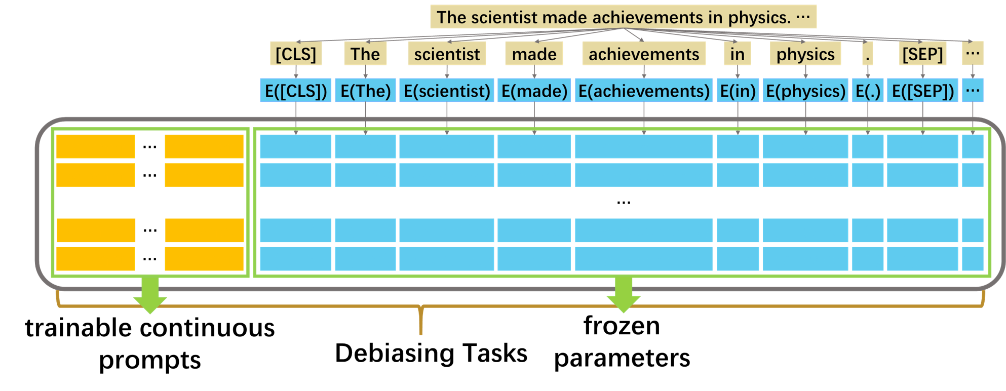
(a) While debiasing, ADEPT only trains the prompt parameters and keeps the base model frozen.

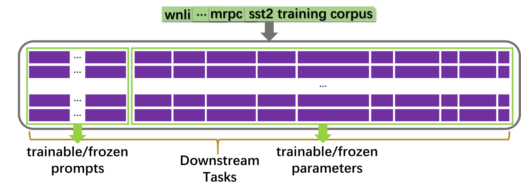
(b) When performing downstream tasks, ADEPT conditions either the base model or both the prompt and the base model.

Figure 1: An illustration of how debiasing works using ADEPT and for downstream tasks.

Natural Language Processing (NLP) tools are widely used today to perform reasoning and prediction by efficiently condensing the semantic meanings of a token, a sentence or a document. As more powerful NLP models have been developed, many real-world tasks have been automated by the application of these NLP systems. However, a great number of fields and tasks have a high demand for fairness and equality: legal information extraction (rabelo2022overview), resume filtering (9799257), and general language assistants (askell2021general) to name a few. Unfortunately, in the pursuit of the most competitive results, folks often blindly apply PLMs, leading to strong performance with the unseen cost of introducing bias into the process. An ideal NLP tool’s decision or choice should not impose harms on a person based on their background (blodgett2020language), but many studies (caliskan2017semantics; mayfield2019equity) have found that biases exist and occur throughout the NLP lifecycle. Thus, it is increasingly important that PLMs can be debiased to enable applications that may be inadvertently influenced by the PLM’s implicit stereotypes.

Debiasing, if treated as a special case of downstream tasks, can be tackled through finetuning. Typically, a finetuning debiasing method puts forward specific loss terms to guide a PLM to remove biases in itself (kaneko2021debiasing). Prompt tuning (li2021prefix; liu2021gpt; lester2021power) is one of the more promising methods for transfer learning with large PLMs these days, and its general success (raffel2020exploring) suggests applications toward debiasing as well. Prompt tuning, whose role is similar to that of finetuning, refers to freezing all the parameters of the original PLM and only training an additional section of parameters (called a “prompt”) for the downstream tasks. Here, a prompt is a set of tokens, often added as a prefix to the input for the task, that act as task-specific complementary information.

All PLM debiasing methods must overcome a major hurdle of “imbalance.” Methods that are imbalanced do not adequately balance eliminating biases in a PLM while maintaining its representation ability. Some existing methods are prone to be destructive, whether destructive refers to decreasing a word/sentence embedding’s projection on a linear bias subspace (liang2020towards), or refers to completely removing the semantic meanings of attribute words (e.g., man, male; and woman, female) from all neutral words (e.g., engineer, scientist; and teacher, librarian) (kaneko2021debiasing). If a debiasing framework focuses only on the PLM’s debiasing task and pays no attention to preserving the model’s useful properties, it may destroy the PLM’s computational structure and counteract the benefits of pretraining altogether. Although an extreme example, a randomly initialized model is expected to be completely unbiased.

In this paper, we propose ADEPT (Figure 1), a debiasing algorithm which implements prompt tuning to debias PLMs and makes the following contributions:

• We are the first to exploit prompt tuning in the debiasing space.

• We introduce a novel debiasing criterion, which often enables the debiased model to perform better than the original one in downstream tasks.

• We show that ADEPT is more effective at mitigating biases on a word embedding manifold than other methods which operate on a linear bias subspace.

• We show methods for improving prototypes for contextualized word embeddings that are generated via aggregation.

Our prompt tuning approach has the inherent advantage of saving computing and storage resources. In our experiments, we achieve great results by training prompts with less than 1% the parameters of the PLM as opposed to fine-tuning approaches which train the whole model. Furthermore, because prompt tuning only trains prompt and the PLM’s original parameters are not touched during the training process, the base model will maintain its robustness.

Related Work

Debiasing Methods

Word Embeddings

Static word embeddings, the foundational building blocks of neural language models, have been a prime target for criticism. In light of artifacts from their training process leading to the encoding of stereotypes, many efforts have been made to mitigate the correlations stored within static embeddings (mikolov2013linguistic; NIPS2016_a486cd07; caliskan2017semantics; mikolov2013efficient; manzini2019black). However, most modern PLMs employ contextualized word embeddings, spreading the potentially biased representations of words across various contexts.

Discrete Prompts

solaiman2021process propose PALMS with Values-Targeted Datasets, which finetunes large-scaled PLMs on a predetermined set of social values in order to reduce PLMs’ biases and toxicity. askell2021general use a hand-designed prompt with more than 4600 solid words as a stronger baseline for helpfulness, harmlessness, and honesty principle for a general language assistant. schick2021self encourage a model to generate biased text and discard its undesired behaviors with this internal knowledge.

In general, discrete prompts debias PLMs in the form of debiasing descriptions. As crafting discrete prompts manually requires domain knowledge and professional expertise, and we cannot ensure hand-crafted prompts’ effectiveness beforehand, we hope to improve debiasing prompts’ performance by transforming it to continuous ones which can be optimized with standard techniques like gradient descent.

Finetuning Setting

kaneko2021debiasing propose a finetuning method of debiasing PLMs. It sets special loss for the debiasing tasks which takes both a PLM’s debiasing results and its expressiveness into account. The experiment shows that token-level debiasing across all layers of the PLM produces the best performance. It further conducts experiments on MNLI tasks and finds that the debiased model preserves semantic information. As this work also makes efforts to maintain a PLM’s expressiveness while debiasing, we take their debiased model as our baseline.

Prompt tuning

Prompt usually has two connotations. One is the text with natural semantics, which is fed into the language model together with the original input as additional information. Another is a set of prefixed, continuous trainable numbers post-set into a PLM, which usually do not have semantic meanings. Because this set of continuous numbers have the same functions as the discrete prompt, such as providing the PLM with extra hints for solving a problem, it is also called prompt (or prefix).

li2021prefix, liu2021gpt, and lester2021power propose prompt tuning (or prefix-tuning, p-tuning) as a lightweight alternative to finetuning for performing downstream tasks. This approach conditions a large-scaled PLM by freezing its original parameters and optimizing a small continuous task-specific embeddings. Besides saving computing and storage resources, prompt tuning performs even better when the PLM scales up and keeps the PLM’s robustness to domain transfer. Our work benefits from these advantages as we debias large PLMs and evaluate their expressiveness on downstream tasks.

Manifold Learning

Manifold learning refers to a series of machine learning methods based on manifold assumption (melas2020mathematical). In order to grasp knowledge from data, we need to hypothesize that data has its inborn structure. Manifold assumption indicates that the observed data lie on a low-dimensional manifold embedded in a higher-dimensional space, for example, a Swiss Roll alike data structure in a 3-dimensional data space. t-SNE (van2008visualizing), a decomposition method based on manifold assumption, provides excellent visualizations for high-dimensional data that lie on several different, but related, low-dimensional manifolds. For word embeddings with high dimensions, we believe we can better describe its distribution with a manifold than with a linear subspace.

Methodology

Algorithm 1 ADEPT: a debiasing algorithm for contextualized word embeddings.

Input: a Pre-trained Language Model (PLM)
Output: $\Phi_{prompt}$ for debiasing the PLM
ADEPT:

1:  Prepare a PLM $M_{\Theta}$ with parameters $\Theta$.

2:  Suppose a bias has $d$ attributes. Define a neutral word tuple $W^{neutral}$ and attribute word tuples $W^{a(i)}=(w_{1}^{a(i)},...,w_{g}^{a(i)})$, each with $g$ one-to-one words.

3:  Collect sentences $S^{neutral}$ and $\{S^{a(i)}\}_{i=1}^{d}$.

4:  Initialize parameters $\Phi_{prompt}$.

5:  for epoch in 1, …, $epoch_{max}$ do

6:     Calculate prototypes of the neutral words: $E^{neutral}=M_{\Theta}^{{}^{\prime}}(S^{neutral})$, where $M_{\Theta}^{{}^{\prime}}=M_{\Theta\cup\Phi_{prompt}}$.

7:     Calculate prototypes of attributes: $E^{a(i)}=M_{\Theta}^{{}^{\prime}}(S^{a(i)}),e^{a(i)}=aver(E^{a(i)})$.

8:     Calculate distances between attribute words and neutral words: $P^{a(i)}=Distance(E^{neutral}|e^{a(i)})$.

9:     Calculate loss of bias: $L_{bias}=\sum_{i,j\in\{1,...,d\},i<j}\{JS(P^{a(i)}||P^{a(j)})\}$.

10:     Calculate loss of representation: $L_{representation}=KL(M_{\Theta}(S)||M_{\Theta}^{{}^{\prime}}(S))$, where $S=S^{neutral}\cup\{S^{a(i)}\}_{i=1}^{d}$.

11:     Calculate the total loss: $L=L_{bias}+\lambda L_{representation}$.

12:     Compute gradient.

13:     Update $\Phi_{prompt}$.

14:  end for

15:  return best $\Phi_{prompt}$

Our goal is: given a PLM $M_{\Theta}$ with parameters $\Theta$, find the parameters $\Phi_{prompt}$ determining a set of continuous prompts, so that the prompt-tuned model $M_{\Theta\cup\Phi_{prompt}}$ (we will use $M_{\Theta}^{{}^{\prime}}$ for short) has the debiasing effects while maintaining the expressiveness of $M_{\Theta}$.

We optimize $\Phi_{prompt}$ by using the objective function:

$$L=L_{bias}+\lambda L_{representation}$$ (1)

where $L_{bias}$ seeks to minimize biases in $M_{\Theta}^{{}^{\prime}}$ whereas $L_{representation}$ caters to the debiased model’s expressiveness, and $\lambda$ is a coefficient to balance the two dependent terms. Our algorithm is summarized in Algorithm 1.

Define Word Tuples and Collect Sentences

We define a neutral word tuple $W^{neutral}$ and several attribute word tuples $W^{a(i)},i=1,...,d$, where the category of bias we are debiasing for contains $d$ different attributes. For example, gender bias may have the attributes “female” and “male,” and here $d=2$ . Words in $W^{neutral}$ are nouns or adjectives that should show no preference for any of the $d$ attributes. For example, “science” and “ambitious,” which should not be bound to any attributes, might be in the tuple $W^{neutral}$. $W^{a(i)}$ denotes a tuple of words where each word is associated attribute $a(i)$ and not $a(j)$ for any $j\neq i$. For example, $W^{male}$ might contain the words “uncle” and “masculine” but not contain the word “science” (since that is a neutral word) or the word “parent” (as this is not specific to the “male” attribute). Next, we enforce that each attribute word tuple is indexed by the same (implicit) indexing set of concepts and that the word at each index is of the same form. For example, if the (implicit) indexing set is (“parent’s sibling”, “parent”, “sibling”) then the male attribute tuple would be (“uncle”, “father”, “brother”) and the female attribute tuple would be (“aunt”, “mother”, “sister”). For brevity, we use the word “pairwise” to describe this correspondence, although the method can be extended to biases with $d>2$ as well.

We then collect sentences based on the word tuples. $S^{neutral}$ (or $S^{a(i)}$) denotes sentences that contain at least one word in $W^{neutral}$ (or $W^{a(i)}$, respectively). Instead of creating template-based sentences using the attribute words from $\{W^{neutral}\}\cup\{W^{a(i)}\}_{i=1}^{d}$, we scrape natural sentences from a corpus (possibly distinct from and/or smaller than the PLM’s pretraining corpus) for a diverse word distribution that aligns better with the real-world.

Calculate Prototypes of Neutral Words/Attributes

To get an insight of a model’s view on different groups, we seek prototypes of neutral words and attributes. To obtain these prototypes, we extract embeddings for each word. For a word from $W^{x}$ ($x$ is $neutral$ or $a(i)$ for some $i$), we fetch the associated sentence from $S^{x}$ and feed it into $M_{\Theta}^{{}^{\prime}}$. Then, we extract the hidden state for the word from each layer of the forward pass. For PLMs adopting WordPiece embeddings such as BERT (devlin2018bert), if a word has several sub-tokens, we average the sub-tokens’ hidden states as the word’s hidden state.

For each word tuple’s sentences $S^{x}$, we extract the set of embeddings $E^{x}$. For attribute words, we follow the procedures from bommasani-etal-2020-interpreting and average the embeddings $E^{a(i)}$ to get a single embedding $e^{a(i)}$ that closer resembles a static embedding as opposed to contextualized embeddings. Under the law of large numbers, we expect this simple linear computation to reduce the context’s linear influences on each attribute word. This process can be summarized as:

$$E^{neutral} =M_{\Theta}^{{}^{\prime}}(S^{neutral})$$ (2)

$$E^{a(i)} =M_{\Theta}^{{}^{\prime}}(S^{a(i)})$$

$$e^{a(i)}=aver(E^{a(i)})$$ (3)

Thus we take $E^{neutral}=[e^{neutral}_{1},e^{neutral}_{2},...]$ as the prototypes of neutral words and $e^{a(i)}$ as the prototype of an attribute.

Define Tuning Loss

We treat word embeddings as being distributed on a manifold and design the loss adhering to the criterion that pairwise attribute words should look alike compared to neutral words on the manifold.

We first design $L_{bias}$ with the intention of pushing pairwise attribute words closer together on the manifold, which corresponds to decreasing biases in a PLM. $p_{n_{j}|a(i)}$ quantifies the degree to which attribute $a(i)$’s information can be restored from the neutral word $n_{j}$ in $M_{\Theta}^{{}^{\prime}}$:

$$p_{n_{j}|a(i)}=\frac{exp(-\frac{||e^{a(i)}-e^{neutral}_{j}||^{2}}{2\rho^{2}})}{\sum_{n_{k}\in W^{neutral}}\{exp(-\frac{||e^{a(i)}-e^{neutral}_{k}||^{2}}{2\rho^{2}})\}}$$ (4)

where $\rho$ is a hyperparameter. We can interpret Equation 4 in this way: (1) Let us set a Gaussian distribution with a covariance matrix to be $\rho$ times the identity matrix at the prototype of attribute $a(i)$, which is $e^{a(i)}$. Then the prototype of the neutral word $n_{j}$, which is $e^{neutral}_{j}$, shows up in the distribution with the probability proportional to $exp(-\frac{||e^{a(i)}-e^{neutral}_{j}||^{2}}{2\rho^{2}})$, the numerator. (2) The denominator sums up the probability mentioned above from all $n_{k}\in W^{neutral}$, and plays a role as the normalization factor. (3) Equation 4 is a formulation that quantifies how much information of $e^{a(i)}$ we can restore from $e^{neutral}_{j}$. Similar equations have been used in other contexts (10.2307/2237880; hinton2002stochastic).

$P^{a(i)}$ denotes our distances from attribute $a(i)$ to all neutral words. $P^{a(i)}=[p_{n_{1}|a(i)},p_{n_{2}|a(i)},...]$ means it is a list of values calculated from $e^{a(i)}$ and $E^{neutral}$. Therefore, we summarize it as below:

$$P^{a(i)}=Distance(E^{neutral}|e^{a(i)})$$ (5)

We define $L_{bias}$ as:

$$L_{bias}=\sum_{i,j\in\{1,...,d\},i<j}\{JS(P^{a(i)}||P^{a(j)})\}$$ (6)

where $JS(P^{a(i)}||P^{a(j)})$ is the Jensen-Shannon divergence between distribution $P^{a(i)}$ and distribution $P^{a(j)}$. This loss term is intended to make up the difference between distinct attributes’ relative distances to the same group of neutral words (in the form of distribution $P^{a(i)}$ and $P^{a(j)}$) so as to push pairwise attribute words closer.

We then design $L_{representation}$ with the intention of maintaining words’ relative distances, which corresponds to maintaining the PLM’s representation ability. $p_{w_{j}|w_{i}}$ quantifies the degree to which the word $w_{i}$’s information can be restored from the word $w_{j}$ in $M_{\Theta}^{{}^{\prime}}$. $P$ denotes the matrix of $p_{w_{j}|w_{i}}$ where $P_{ij}=p_{w_{j}|w_{i}}$. For $q_{w_{j}|w_{i}}$ and $Q$, they denote likewise except that the model is the original one $M_{\Theta}$. $p_{w_{j}|w_{i}}$ and $q_{w_{j}|w_{i}}$ have the same definition as in Equation 4.

We define $L_{representation}$ as:

$$L_{representation} =KL(Q||P)$$ (7)

$$=\sum_{i=1}^{||V||}\sum_{j=1}^{||V||}Q_{ij}log_{2}(\frac{Q_{ij}}{P_{ij}})$$

where $||V||$ denotes vocabulary size.

In Algorithm 1, we write $L_{representation}$ as:

$$L_{representation}=KL(M_{\Theta}(S)||M_{\Theta}^{{}^{\prime}}(S))$$ (8)

where S denotes the union of $S^{neutral}$ and $\{S^{a(i)}\}_{i=1}^{d}$. Here the $L_{representation}$ aims to keep the PLM’s parameters unchanged. Rather than using $L_{2}$ norm to gauge how much the outputs of the debiased model has changed as kaneko2021debiasing do, we measure the differential between the original model’s hidden states and the debiased model’s hidden states with KL divergence. $L_{representation}$ in Equation 8 is more time-efficient for training and evaluation tasks than the one in Equation 7, so we adopt it in ADEPT.

Improve Prototypes of Attributes

After we confirm that Algorithm 1 works, we make efforts to improve prototypes of attributes $e^{a(i)}$ by adjusting properties of $S^{a(i)}$. We can tell from Equation 3 that $e^{a(i)}$ is a calculated prototype with intuitive correctness. Therefore, we implement experiments on deciding on the desirable properties of $S^{a(i)}$ regarding its reliability, quality and quantity, altering single variable at a time, to check whether $e^{a(i)}$’s expressiveness can be improved with the modified $S^{a(i)}$. The test granularity extends from a single word to the whole attribute.

$S^{a(i)}_{m}$ denotes a sub-list of $S^{a(i)}$ composed with sentences that contain $w^{a(i)}_{m}$, where $w^{a(i)}_{m}$ means the $m^{th}$ item of tuple $W^{a(i)}$. $len(S^{a(i)}_{m})$ and $len(S^{a(i)})$ denote the length of the lists.

Reliability

Here, the experiment is devised to answer: if $len(S^{a(i)}_{m})$ is less than a threshold, shall we take the word $w^{a(i)}_{m}$ as a contributing word for constructing $e^{a(i)}$? To satisfy the law of large number, we set the threshold to be 30.

Quality

Here, the experiment is devised to answer: if $len(S^{a(1)}_{m})\neq len(S^{a(2)}_{m})\neq...$, which is often the case, will this disproportion of pairwise words affect $e^{a(i)}$’s expressiveness? We set $len(S^{a(1)}_{m})=len(S^{a(2)}_{m})=...,m\in[1,g]$ and compare the results.

Quantity

Here, the experiment is devised to answer: whether for $len(S^{a(i)})$, the larger, the better? We conduct the tests with the $len(S^{a(i)})$ being of a different order of magnitude.

Experiments

Datasets, Benchmarks and Baselines

For the word tuples, we use neutral word lists employed in previous debiasing methods (kaneko2021debiasing; caliskan2017semantics). For the binary gender setting, we use the pairwise attribute words from zhao2018learning and for the ternary religion setting, we use the attribute triplets from liang2020towards. For the sentences associated with the word tuples, we draw sentences from News-Commentary v15 (TIEDEMANN12.463) for the gender setting and sentences from BookCorpus (Zhu_2015_ICCV) and News-Commentary v15 (TIEDEMANN12.463) for the relgions setting. Since the original BookCorpus is no longer available, we use (bookcorpus_hf) which is an open source replica. We use this corpus since BookCorpus is part of the corpus BERT is originally trained on. In total, for the gender setting, we draw 20,710 neutral sentences and 44,683 sentences each for the male and female attributes. For the religion setting, we draw 73,438 neutral sentences and 5,972 sentences corresponding to each attribute (Judaism, Christianity, and Islam).

We evaluate gender stereotype scores on SEAT 6, 7, 8 (may2019measuring) and CrowS-Pairs (nangia2020crows), widely-used benchmarks/metrics designed to evaluate a model’s biases toward/against different social groups. We evaluate the debiased models’ representation ability on selected GLUE (wang2018glue) tasks, each of which is with little training data: Stanford Sentiment Treebank (SST-2, (socher-etal-2013-recursive)), Microsoft Research Paraphrase Corpus (MRPC, (dolan-brockett-2005-automatically)) Recognizing Textual Entailment (RTE, (dagan2005pascal; haim2006second; giampiccolo2007third; bentivogli2009fifth)) and Winograd Schema Challenge (WNLI, (levesque2012winograd)). We further evaluate the comprehensive performance of the debiased model pertaining to its biases and expressiveness on a filtered portion of the StereoSet-Intrasentence data (nadeem2020stereoset), employing 149 test examples for the gender domain and 5,770 test examples overall.

We compare our algorithm with Debiasing Pre-trained Contextualised Embeddings (DPCE; (kaneko2021debiasing)), a similar method that focuses on making the neutral words’ embeddings devoid of information in relation to a protected attribute by finetuning the model with the loss term being the sum of the inner product between the attribute words’ hidden states and the neutral words’ hidden states.

Hyperparameters

We conduct experiments on the bert-large-uncased pre-trained model from HuggingFace (wolf2019huggingface). By using ADEPT, we need only train 1.97M parameters when prompt-tuning with 40 prompt tokens, orders of magnitude smaller than the 335M parameters required for finetuning.

We set $\lambda$ in Equation 1 to be $\frac{7}{3}$ and $\rho$ in Equation 4 to be 15. We use Adam (kingma2014adam) to optimize the objective function. During the debiasing process, our learning rate is 5e-5 and our batchsize is 32. Results for DPCE are using the hyperparameters originally reported in kaneko2021debiasing. All the experiments are conducted on two GeForce RTX 3090 GPUs and in a Linux operating system.

Bias Benchmarks

We use three main benchmarks for evaluating performance vis-a-vis bias.

SEAT

The Sentence Encoder Association Test (SEAT) (may2019measuring) extends the Word-Embedding Association Test (WEAT) (caliskan2017semantics) to the sentence-level by filling hand-crafted templates with the words in WEAT. In this way, SEAT aims to measure biases in sentence-encoders like ELMo (peters-etal-2018-deep) and BERT (devlin2018bert) as opposed to only the biases in word embeddings. The SEAT benchmark provides two scores, namely effect size and P-value, where an effect size with smaller absolute value is regarded as a better score for a debiased model.

CrowS-Pairs

CrowS-Pairs (nangia2020crows) features pairwise test sentences, differing only in a stereotyped word and an anti-stereotyped word in the same position. This benchmark evaluates whether a PLM will assign a higher probability to a stereotyped sentence than to an anti-stereotyped one where the probability is assigned while attempting to account for differing priors. A ideal model will get the score of 50.

StereoSet

StereoSet (nadeem2020stereoset) measures both a PLM’s useful semantic information as well as its biases by using cloze tests. Provided a brief context, a PLM must choose its preference from a stereotype, an anti-stereotype, and an unrelated choice. A higher, up to 100, Language Modeling Score (LMS) indicates better expressiveness, and a Stereotype Score (SS) closer to 50 indicates less biases. The Idealized CAT Score (ICAT) is a combined score of LMS and SS with the best score being 100.

Results and Analysis

	original	DPCE	ADEPT-finetuning	ADEPT
C6: M/F Names, Career/Family	0.369	0.936	0.328	0.120
C7: M/F Terms, Math/Arts	0.418	-0.812	-0.270	-0.571
C8: M/F Terms, Science/Arts	-0.259	-0.938	-0.140	0.132
CrowS-Pairs: score(S)	55.73	47.71	52.29	48.85
GLUE: SST-2	92.8	92.8	93.6	93.3	92.7
GLUE: MRPC	83.1	70.3	83.6	84.6	85.0
GLUE: RTE	69.3	61.0	69.0	69.7	69.7
GLUE: WNLI	53.5	45.1	46.5	47.9	56.3
StereoSet(filtered)-gender: LMS	86.338	84.420	86.005	84.652
StereoSet(filtered)-gender: SS	59.657	59.657	57.113	56.019
StereoSet(filtered)-gender: ICAT	69.663	68.115	73.770	74.462
StereoSet(filtered)-overall: LMS	84.162	58.044	84.424	83.875
StereoSet(filtered)-overall: SS	58.243	51.498	57.701	55.435
StereoSet(filtered)-overall: ICAT	70.288	56.305	71.420	74.759

Table 1: Evaluation results on debiasing performance. We test the debiased models on SEAT (from row 1 to 3), CrowS-Pairs (row 4), GLUE (from row 5 to 8) and filtered StereoSet-Intrasentence (from row 9 to 14), with best result in bold. original, the original bert-large-uncased model; DPCE (kaneko2021debiasing), the baseline model; ADEPT-finetuning, model finetuned with our new debiasing criterion; ADEPT, model tuned with ADEPT. As for downstream tasks in GLUE, we test ADEPT on both fine-tuning the original model only (left) and fine-tuning the model as well as the debiasing prompt (right).

We evaluate four models on all benchmarks, namely the original model (pre-trained with no explicit debiasing), the DPCE model, the ADEPT-finetuning model finetuned following our debiasing criterion, and the ADEPT model (ours). For the CrowS-Pairs and StereoSet experiments, we inherit the classifier from the bert-large-uncased model to predict the masked token, so we perform CrowS-Pairs and StereoSet evaluations on the model with the slightest change. As a result, we choose ADEPT model with 500 training steps in these two benchmarks’ evaluation. For SEAT and GLUE, we use the ADEPT model after 10 epochs of training.

Reducing Biases

In Table 1, experiments show that ADEPT achieves competitive debiasing results, outperforming DPCE and mostly obtaining the best scores of the four models on SEAT and CrowS-Pairs. ADEPT-finetuning, which shifts ADEPT from the prompt-tuning setting to a finetuning setting, is also broadly successful at eliminates biases in PLMs. More trainable parameters notwithstanding, ADEPT-finetuning fails to beat ADEPT, implying that debiasing does not require a great change to the original model.

Preserving Representation Ability

In Table 1, the GLUE tests show that ADEPT does not harm the model’s representation ability and even improves it in most cases, with increased scores on SST-2, MRPC, and RTE. As shown in Figure 1LABEL:sub@1-b, after being debiased with ADEPT, the model can choose from training the base model or both the prompt and the base model when performing downstream tasks, and we test both on selected GLUE tasks. Notably, the trainable prompt parameters account for less than 1/100 of the base model parameters, so additionally training the prompts does not significantly add to the computational burden. We can see enhanced performance in both cases. ADEPT-finetuning also manages to outperform the original pre-trained model on SST-2 and MRPC, although the overall results are less noteworthy.

Visualization and Comprehensive Performance

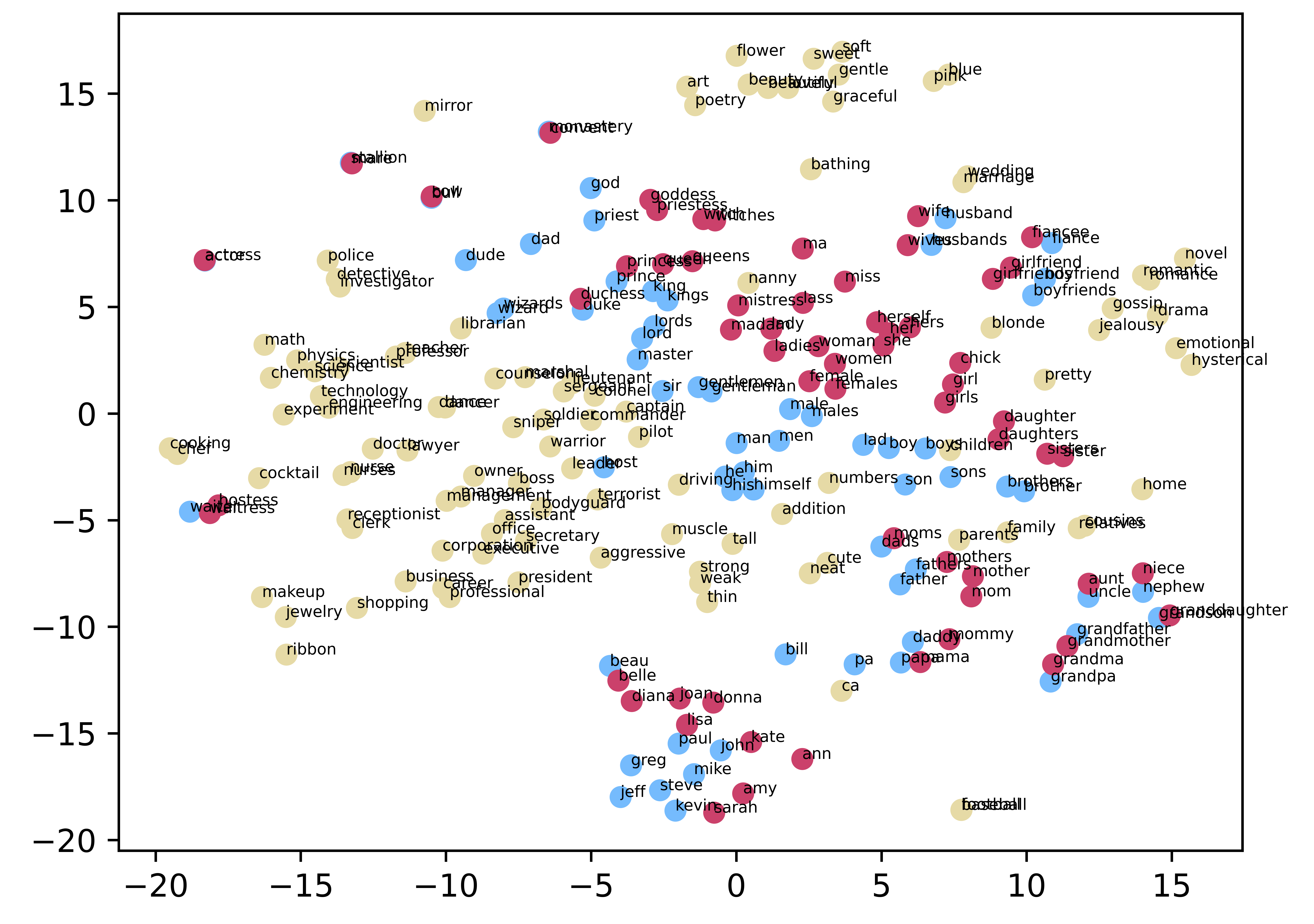
(a) original

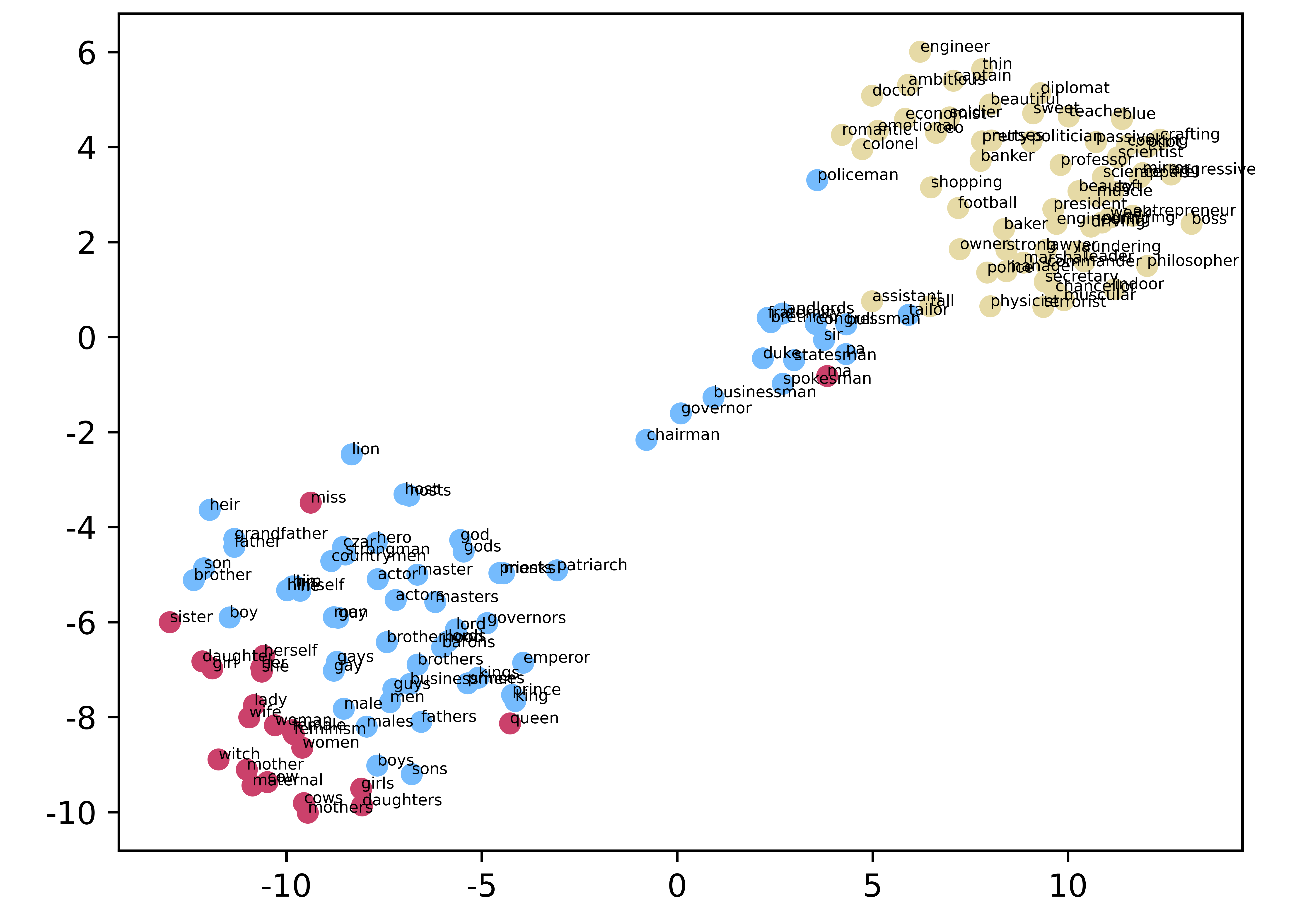
(b) DPCE

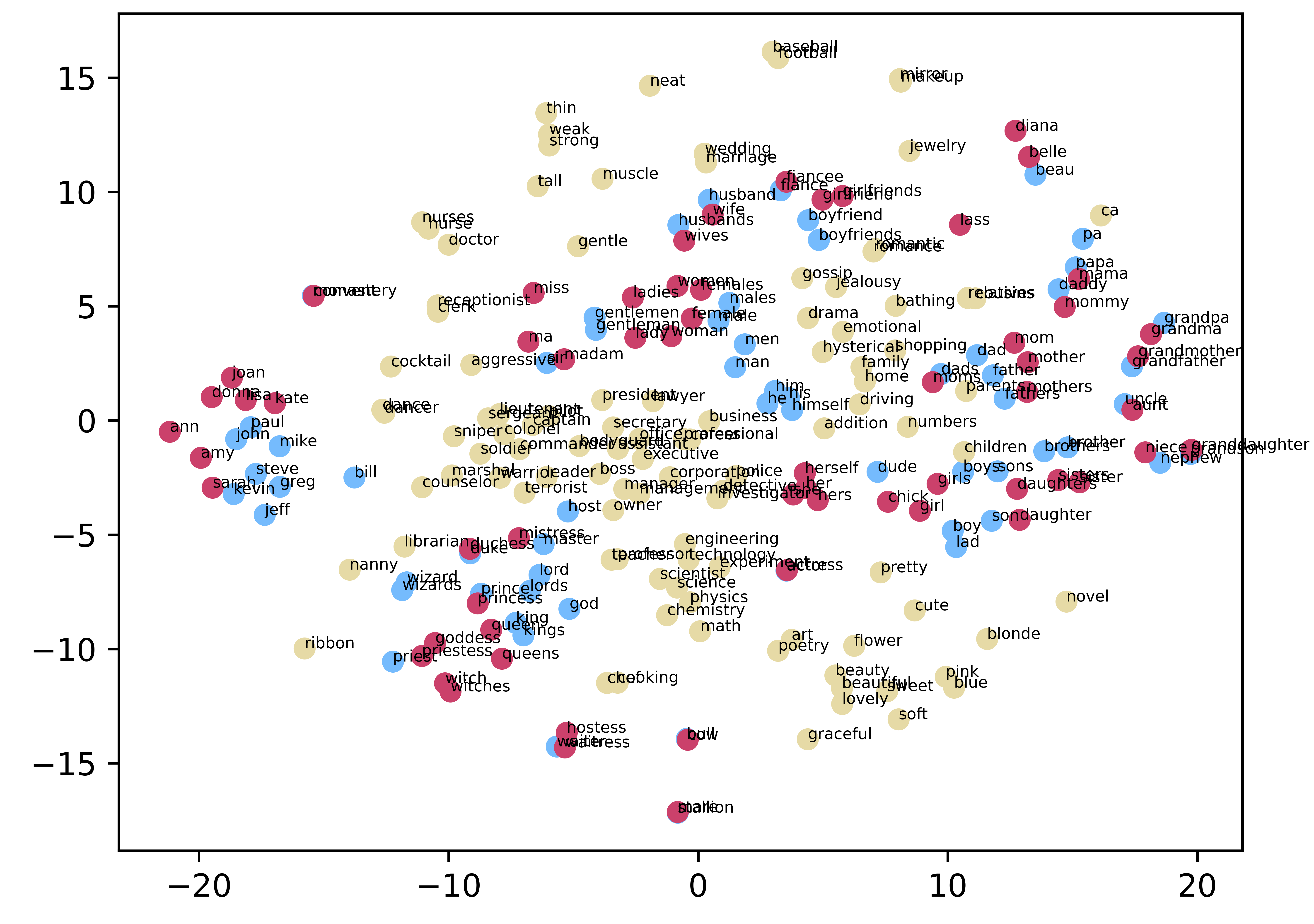
(c) ADEPT-finetuning

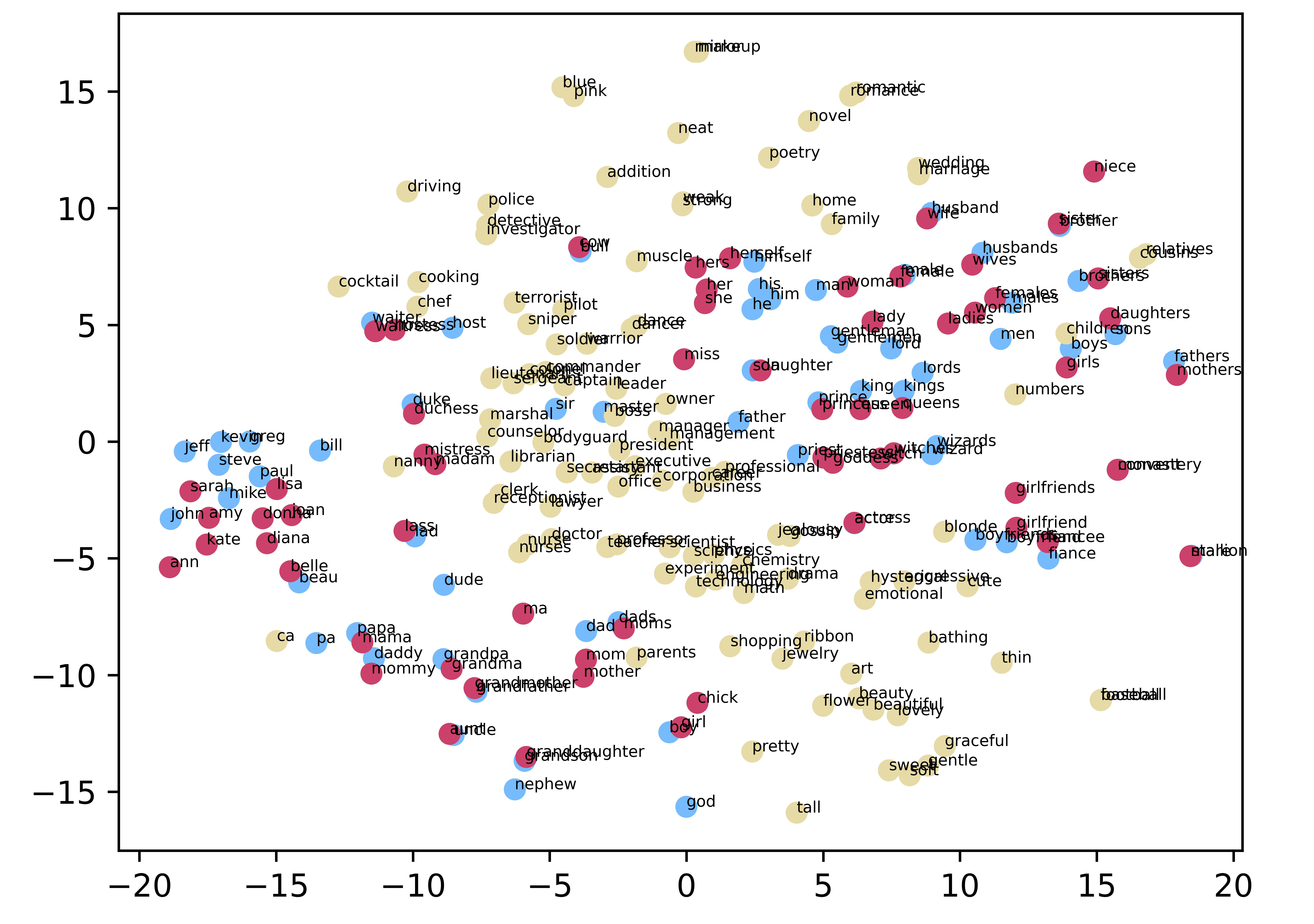
(d) ADEPT

Figure 2: Visualized correlation of words in the gender domain. We use t-SNE to plot the figures and set perplexity as 30. We color neutral words beige, male words blue, and female words red.

We explore the visible increase in the debiased model’s expressiveness by visualizing words’ correlation given by the model before and after debiasing, and provide a comprehensive score on the filtered StereoSet-Intrasentence. For a better prototype of a word, we average the last layer hidden state of the word from 30 different sentences. We plot ADEPT’s performance on binary gender debiasing in Figure 2LABEL:sub@2-d (we also plot the results for ternary religion debiasing in the Appendix). We filter the StereoSet-Intrasentence dataset to only keep test examples with the target words “daddy,” “ma’am,” “groom,” “bride,” “stepfather,” or “stepmother,” as these words show up less often in the tuning corpus.

From Figure 2 we can conclude that ADEPT succeeds at maintaining words’ relative distances, while simulatenously pulling pairwise attribute words closer. In comparison, as shown in Figure 2LABEL:sub@2-b, removing attribute semantic meanings as done in DPCE splits neutral words and gender words apart, which actually makes the difference between pairwise gender words negligible compared to their relative distances to the neutral words group. This may account for why some previous debiasing methods see a drastic drop in their model’s expressiveness after debiasing whereas ADEPT does not. We further plot the evaluation loss in the training process in Appendix and find that the training process of ADEPT is smoother than that of DPCE.

The filtered StereoSet-Intrasentence result also implies that ADEPT is better at keeping useful semantic information when eliminating biases. ADEPT achieves the best ICAT score across the evaluated models in the filtered StereoSet-Intrasentence for gender and for overall, with best SS in gender domain and best LMS across domains. The baseline DPCE model appears to misunderstand words other than gender words as its LMS declines from 84 to 58 when the StereoSet-Intrasentence extends its examples from gender to other protected groups like race and religion. We note that the SS does not improve as much as the SEAT or CrowS-Pairs scores do. We hypothesize that this is because our training process is more similar to the metrics used for SEAT and CrowS-Pairs, which are calculated across the full sentence, rather than to StereoSet, which computes only for the word.

Experiments for Improving Prototypes of Attributes

	LMS	SS	ICAT	score(S)
raw	86.674	62.341	65.282	52.29
reliability	85.975	61.846	65.605	53.05
quality	86.728	62.329	65.343	53.44
quantity-100	86.493	60.857	67.712	53.82
quantity-1000	86.166	61.168	66.920	51.91
quantity-10000	86.753	61.550	66.713	52.29

Table 2: Experiment results on desirable properties of $S^{a(i)}$ as detailed in the section on Improving Prototypes.

We feed all sentences in $S^{a(i)}$ into the PLM, average the hidden states of the attribute words, and get a prototype $e^{a(i)}$ of attribute $a(i)$ on the manifold. As we aim to drive pairwise attribute words closer on the manifold, a prototype has to be clear and precise for generalizing the attribute’s concept. Therefore, we perform several experiments adjusting the properties of $S^{a(i)}$ to improve $e^{a(i)}$. raw denotes the original $S^{a(i)}$.

Reliability

As contextualized word embeddings mix context information into every token’s hidden states, for word $w^{a(i)}_{m}$, we need a myriad of context sentences to construct its prototype. Therefore, we regard $S^{a(i)}_{m}$ with $len(S^{a(i)}_{m})<30$ as unreliable, and remove them from $S^{a(i)}$.

Quality

Pairwise attribute words, like “waiter” and “waitress” for gender, should make equal contributions to the prototype. For a word $w^{a(i)}_{m}$, if its $S^{a(i)}_{m}$ makes up most of the $S^{a(i)}$, then the calculated prototype may well be influenced by the word’s semantic meaning and leads to ambiguity. Thus, we enforce $len(S^{a(1)}_{m})=len(S^{a(2)}_{m})=...$ for all pairwise attribute words.

Quantity

A larger corpus indicates more diverse training sentences and attribute words, but is more time-consuming to train. Hence, we test $S^{a(i)}$ with sizes at different orders of magnitude and compare the effects to choose the most desirable corpus size.

We run ADEPT-finetuning on the corpora mentioned above, stop the training at 500 steps (an early stage), and evaluate the debiased models on StereoSet-Intrasentence and CrowS-Pairs. Results are listed in Table 2. Data show that setting threshold for $S^{a(i)}_{m}$ and slicing pairwise $S^{a(i)}_{m}$ to be of equal size help improve the performance. In our experiments, we filter $S^{a(i)}_{m}$ if $len(S^{a(i)}_{m})<30$, set $len(S^{a(1)}_{m})=len(S^{a(2)}_{m})=...$ and choose quantity-10000.

Conclusion

We proposed ADEPT, an algorithm that adopts prompt tuning for debiasing and introduces a new debiasing criterion inspired by manifold learning. By using prompt tuning, ADEPT consumes less computing and storage resources while preserving the base model’s parameters, ensuring the model’s robustness for other tasks after debiasing. Using this new debiasing criterion, ADEPT obtains competitive scores on bias benchmarks and even improves a PLM’s representation ability for downstream tasks. By visualizing the words’ correlation before and after the PLM is debiased, we find that ADEPT drives pairwise attributes closer on the manifold and keeps words’ relative distances. ADEPT provides a smoother loss function than previous methods, allowing for better use of optimizations like early stopping. We also establish the standard of evaluating the corpus for building attribute prototypes in the contextualized word embedding setting and refine ADEPT’s performance with it. In the future, we will explore time-efficient objective terms for keeping words’ relative distances in debiasing and release a new dataset that measures a model’s biases and expressiveness comprehensively, free of the need to make predictions about masked tokens.

Ethics Statement

When designing ADEPT, we made some assumptions to simplify the complex world model which may lead to some ethical concerns.

We defined bias in this paper as the difference between attribute prototypes relative to neutral words. However, this requires carefully selecting the categories of the attribute based on real-world debiasing demands. Unfortunately, our construction could be reversed such that the words in the attributes list are made as different in distance from the neutral words as possible, but we expect that this would cause the embeddings to degrade and thus not be effective for intentionally causing harm.

In our paper, we discussed the usage of ADEPT on the binary gender setting, which in general is not reflective of the real world, where gender (and other biases) can be far from binary. It is reasonable to have concerns that a binary construction can cause harms to groups not part of the pair. Luckily, all pieces of ADEPT are directly extensible to any number of dimensions, allowing for all dimensions to be pushed to cluster together.

Unfortunately, we cannot ensure or contradict causality between bias reduction and discrimination mitigation in PLMs. goldfarb2020intrinsic makes an effort to deny the causality between bias and discrimination, but it only takes WEAT as the intrinsic task, so more work is needed in this area to ensure that we are indeed reducing harms.

References

* 9799257.
rabelo2022overview.
askell2021general.
blodgett2020language.
mikolov2013linguistic.
NIPS2016_a486cd07.
caliskan2017semantics.
mayfield2019equity.
manzini2019black.
mikolov2013efficient.
dai2015semi.
devlin2018bert.
radford2018improving.
yang2019xlnet.
may2019measuring.
nangia2020crows.
nadeem2020stereoset.
zmigrod2019counterfactual.
liang2020towards.
schick2021self.
meade2021empirical.
kaneko2021debiasing.
raffel2020exploring.
li2021prefix.
liu2021gpt.
lester2021power.
liu2021p.
solaiman2021process.
guo-etal-2022-auto.
peters-etal-2018-deep.
melas2020mathematical.
bommasani-etal-2020-interpreting.
10.2307/2237880.
hinton2002stochastic.
kaneko-bollegala-2019-gender.
zhao2018learning.
TIEDEMANN12.463.
Zhu_2015_ICCV.
bookcorpus_hf.
wang2018glue.
socher-etal-2013-recursive.
dolan-brockett-2005-automatically.
dagan2005pascal.
haim2006second.
giampiccolo2007third.
bentivogli2009fifth.
levesque2012winograd.
wolf2019huggingface.
kingma2014adam.
goldfarb2020intrinsic. aaai23

Appendix

(a) original

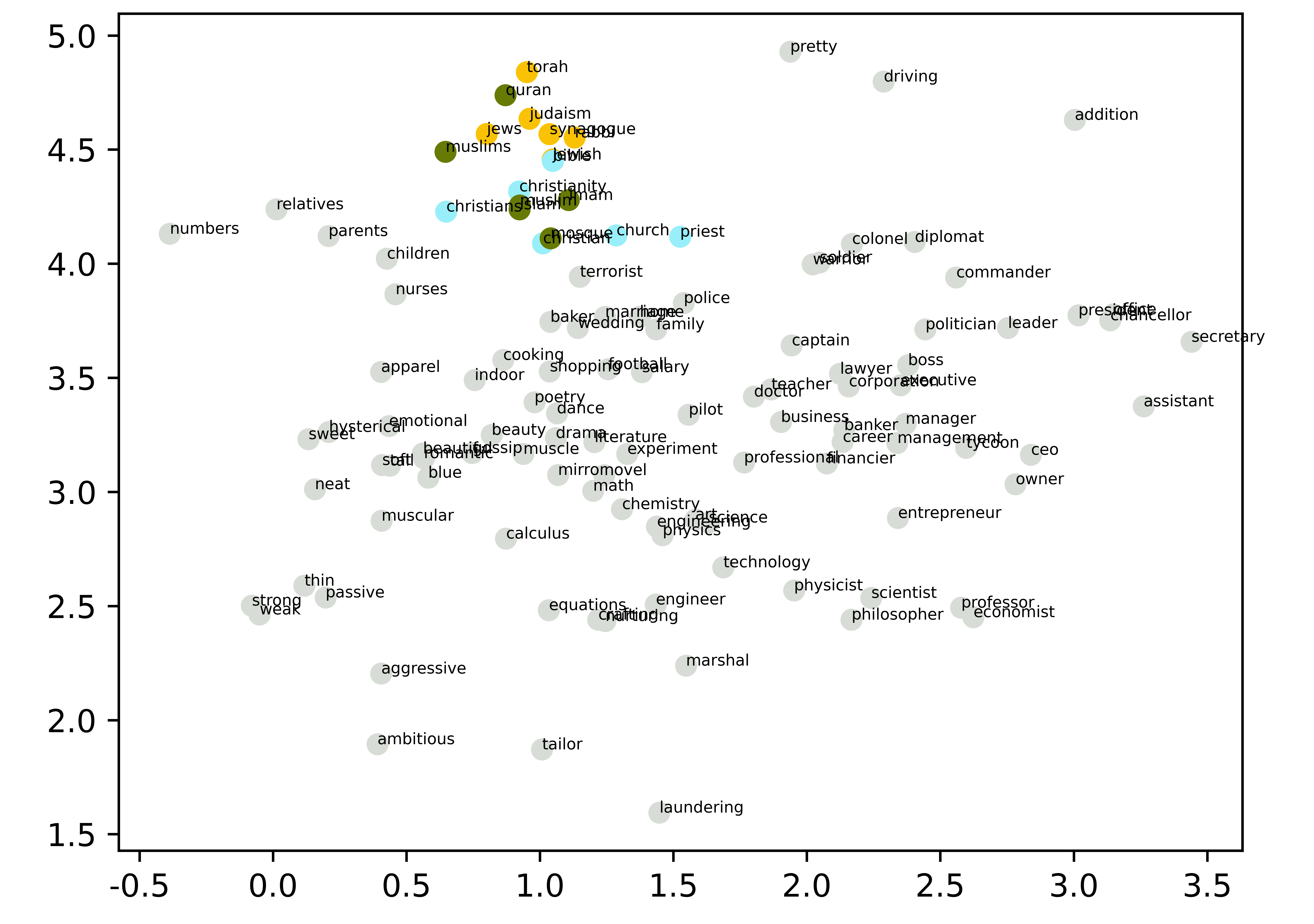
(b) ADEPT

Figure 3: Visualized correlation of words in the religion domain. We use t-SNE to plot the figures and set perplexity as 80. We color neutral words grey, Judaism words yellow, Christianity words blue, and Islam words green.

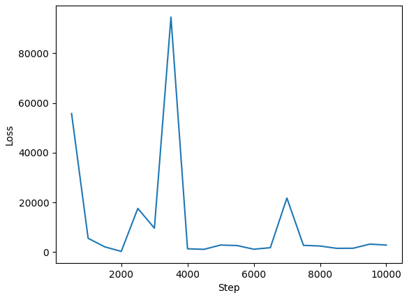
(a) DPCE

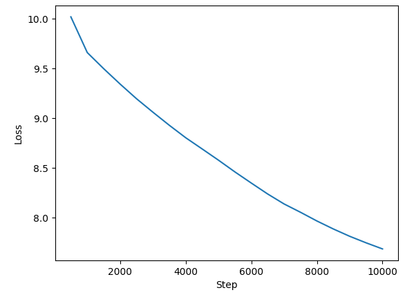
(b) ADEPT

Figure 4: Evaluation loss in the training processes for DPCE and ADEPT.

Further Explanations for Figures in Appendix

As is depicted in Figure 3LABEL:sub@3-a, we visualize the words’ correlation given by the original model, and find that attribute words in each religious group cluster together, and Christianity words appear closer to neutral words than the other two groups. Moreover, the word “terrorist” shows up alongside Islam words with the shortest distance between any neutral word and any religious attributes, implying an undesirable association for Islamists.

Words’ correlation in Figure 3LABEL:sub@3-b displays that after debiasing with ADEPT, ternary religious words get closer, like for the case of “torah,” “bible,” and “quran,” and therefore they look more similar to neutral words. If we go into details, the word “terrorist” hardly shows preference for any religious attributes this time.

Figure 4LABEL:sub@4-b portrays a gracefully declining evaluation loss of ADEPT during the debiasing process. For Figure 4LABEL:sub@4-a, we doubt if it is the high learning rate as is suggested in the DPCE work that leads to the unstable evaluation loss, so we reduce the learning rate to 5e-6 and replicate the SEAT tests for the new debiased (with DPCE) model. New results show that the evaluation loss remains unsettled but the SEAT scores collapse, and as a result, we stick to the original learning rate for DPCE’s training and evaluation.

References

*
\bibentry9799257.
\bibentryrabelo2022overview.
\bibentryaskell2021general.
\bibentryblodgett2020language.
\bibentrymikolov2013linguistic.
\bibentryNIPS2016_a486cd07.
\bibentrycaliskan2017semantics.
\bibentrymayfield2019equity.
\bibentrymanzini2019black.
\bibentrymikolov2013efficient.
\bibentrydai2015semi.
\bibentrydevlin2018bert.
\bibentryradford2018improving.
\bibentryyang2019xlnet.
\bibentrymay2019measuring.
\bibentrynangia2020crows.
\bibentrynadeem2020stereoset.
\bibentryzmigrod2019counterfactual.
\bibentryliang2020towards.
\bibentryschick2021self.
\bibentrymeade2021empirical.
\bibentrykaneko2021debiasing.
\bibentryraffel2020exploring.
\bibentryli2021prefix.
\bibentryliu2021gpt.
\bibentrylester2021power.
\bibentryliu2021p.
\bibentrysolaiman2021process.
\bibentryguo-etal-2022-auto.
\bibentrypeters-etal-2018-deep.
\bibentrymelas2020mathematical.
\bibentrybommasani-etal-2020-interpreting.
\bibentry10.2307/2237880.
\bibentryhinton2002stochastic.
\bibentrykaneko-bollegala-2019-gender.
\bibentryzhao2018learning.
\bibentryTIEDEMANN12.463.
\bibentryZhu_2015_ICCV.
\bibentrybookcorpus_hf.
\bibentrywang2018glue.
\bibentrysocher-etal-2013-recursive.
\bibentrydolan-brockett-2005-automatically.
\bibentrydagan2005pascal.
\bibentryhaim2006second.
\bibentrygiampiccolo2007third.
\bibentrybentivogli2009fifth.
\bibentrylevesque2012winograd.
\bibentrywolf2019huggingface.
\bibentrykingma2014adam.
\bibentrygoldfarb2020intrinsic.
\nobibliographyaaai23