Controlling Moments with Kernel Stein Discrepancies

Abstract

Kernel Stein discrepancies (KSDs) measure the quality of a distributional approximation and can be computed even when the target density has an intractable normalizing constant. Notable applications include the diagnosis of approximate MCMC samplers and goodness-of-fit tests for unnormalized statistical models. The present work analyzes the convergence control properties of KSDs. We first show that standard KSDs used for weak convergence control fail to control moment convergence. To address this limitation, we next provide sufficient conditions under which alternative diffusion KSDs control both moment and weak convergence. As an immediate consequence we develop, for each $q>0$, the first KSDs known to exactly characterize $q$-Wasserstein convergence.

1 Introduction

We consider the problem of estimating the expectation $\mathbb{E}_{P}[f]=\int f(x)\differential P(x)$ of a function $f$ on $\mathbb{R}^{d}$ with respect to a probability distribution $P.$ We will focus on the case where $P$ is defined by a density function with an unknown normalization constant, so that exact computation of the expectation is intractable. In this case, we must resort to approximation.

Numerical integration techniques have been extensively studied for this purpose. One well-known, general method is Markov Chain Monte Carlo (MCMC) (Casella and Berger, 2002), which produces estimates in the form of a weighted sum $\mathbb{E}_{Q}[f]=n^{-1}\sum_{i=1}^{n}f(x_{i}).$ Another example is variational Bayesian methods (Blei et al., 2017), which are specifically designed for Bayesian posterior distributions. Regardless of the type of the method used, quantifying the quality of approximation is desirable, since we can then diagnose and compare (competing) methods to obtain more accurate estimates.

This problem may be approached using Stein discrepancies, a class of measures of discrepancy between probability distributions (Gorham and Mackey, 2015). The key idea behind a Stein discrepancy is that we can construct functions that are integrated to zero under the target distribution; such functions may be used to measure the discrepancy of another distribution, since a non-zero expectation under the distribution indicates its deviation from the target. Formally, a Stein discrepancy of a distribution $Q,$ with respect to target $P,$ is defined as the worst-case quantity

$$\sup_{g\in{\cal{\cal G}}}\left|\mathbb{E}_{Q}[{\cal T}_{P}g]\right|,$$

where ${\cal T}_{P}$ and ${\cal G}$ are a Stein operator and a Stein set (a function class in the domain of ${\cal T}_{P}$), inducing functions ${\cal T}_{P}g$ whose expectations vanish under $P.$ Different choices of the operator and the function class yield distinct Stein discrepancies. A prototypical example is the Langevin Stein operator (Gorham and Mackey, 2015; Oates et al., 2017), which may be defined without the normalization constant; and two major classes based on this operator are the graph Stein discrepancies (Gorham and Mackey, 2015; Gorham et al., 2019) and the kernel Stein discrepancy (KSD) (Chwialkowski et al., 2016; Liu et al., 2016; Oates et al., 2017; Gorham and Mackey, 2017). Notably, it is possible to compute these discrepancies: the KSD circumvents the supremum in the definition and admits a closed-form expression involving kernel evaluations on samples, whereas the graph Stein discrepancy involves solving a linear program. This computational advantage has sparked numerous statistical applications involving unnormalzed densities (see the survey by Anastasiou et al., 2023, for an overview).

While successfully avoiding the intractable expectation, Stein discrepancies may not be immediately interpreted in terms of the expectation $\mathbb{E}_{P}[f]$ of interest. Prior work therefore investigated how Stein discrepancies characterize closeness in expectation under suitable regularity conditions on the integrand. With the exception of Barp et al. (2022), the foregoing studies used Stein’s method (Stein, 1972) to relate Stein discrepancies to integral probability metrics (IPMs) (Müller, 1997), which measure the worst-case difference in expectations with respect to given classes of functions. Gorham and Mackey (2015) showed that the Langevin graph Stein discrepancy controls the 1-Wasserstein distance (the IPM defined by $1$-Lipschitz functions) for distantly dissipative target distributions; Gorham et al. (2019) later generalized this result to heavy-tailed targets with diffusion graph Stein discrepancies. Gorham and Mackey (2017) proved that the Langevin KSD with the inverse multi-quadratic kernel (IMQ) controls the bounded-Lipschitz metric; Chen et al. (2018) offer other kernel choices. Random feature Stein discrepancies by Huggins and Mackey (2018) control the bounded-Lipschitz metric with appropriate features, while being computable in linear time. Using a distinct approach from the aforementioned works, Barp et al. (2022) showed that the separating property of the KSD is equivalent to having (tight) weak convergence control (i.e., convergence in expectations of bounded continuous functions).

Statistical analysis often involves unbounded functions; e.g., basic statistical measures such as mean and variance are the expectation of linear and quadratic functions. That said, it remains an open question to which class of unbounded integrands, Stein discrepancies are guaranteed to indicate the quality of expectation approximations. This question has been in part tackled by works on graph Stein discrepancies (Gorham and Mackey, 2015; Gorham et al., 2019). These analyses, however, are limited to linearly growing functions – it is unclear how these results extend to functions of faster growth. Moreover, despite its computational appeal over the graph Stein discrepancies, the KSD has only been shown to control weak convergence.

This article aims to extend the reach of the KSD to functions of arbitrary polynomial growth. In particular, we investigate conditions under which the KSD controls the convergence of expectations of polynomially growing continuous functions ($q$-Wasserstein convergence, defined formally in Section 3.1). Our specific contributions are threefold. First, our analysis considers the diffusion kernel Stein discrepancy (Barp et al., 2019), a generalization of the Langevin KSD (Chwialkowski et al., 2016; Liu et al., 2016; Oates et al., 2017; Gorham and Mackey, 2017). This extension allows us to consider a broader target class, including heavy-tailed distributions, for which the Langevin KSD has proved inadequate to control weak convergence (Gorham and Mackey, 2017; Barp et al., 2022). Second, we show that standard KSDs used for controlling weak convergence fail to control moment convergence. As our third contribution, we address this limitation by identifying, for the first time, specific practical reproducing kernels that provide polynomial convergence control. Consequently, we establish the first Stein discrepancies known to exactly control $q$-Wasserstein convergence for each $q>0$.

The rest of the article is organized as follows. Section 2 introduces the KSD and its associated Stein operator. Section 3 presents the motivating negative result of standard KSDs, followed by two main results addressing this shortcoming. In Section 3.1, our first result, building on the work of Barp et al. (2022), establishes sufficient conditions on the kernel to facillitate the control of $q$-Wasserstein convergence by the KSD. In Section 3.2, building on the finite Stein factor results of Erdogdu et al. (2018), our second result provides an explicit KSD upper bound on the IPM defined by a class of pseudo-Lipschitz functions, a polynomial generalization of Lipschitz functions. This bound enables us to describe a rate of Wasserstein convergence in terms of the KSD. Our experiments in Section 4 confirm the claimed convergence control property. We conclude in Section 5.

Notation and definitions

We define the inner product between multi-dimensional arrays $A,B\in\mathbb{R}^{d_{1}\times\dots\times d_{n}}$ by the sum of the elementwise product $\sum A_{i_{1},\dots,i_{n}}B_{i_{1},\dots,i_{n}}$, where $A_{i_{1},\dots,i_{n}}$ and $B_{i_{1},\dots,i_{n}}$ are the $(i_{1},\dots,i_{n})$-entry of the respective arrays. For $A\in\mathbb{R}^{d_{1}\times\dots\times d_{n}}$, we define its Frobenius norm by $\lVert A\rVert_{\mathrm{F}}=\sqrt{\langle A,A\rangle}$ and its operator norm by

$$\lVert A\rVert_{\mathrm{op}}\coloneqq\sup_{\lVert u^{(1)}\rVert_{2}=\cdots=\lVert u^{(n)}\rVert_{2}=1}\lvert\langle A,u^{(1)}\otimes\cdots\otimes u^{(n)}\rangle\rvert,$$

where $u^{(1)}\otimes\cdots\otimes u^{(n)}\in\mathbb{R}^{d_{1}\times\cdots\times d_{n}}$ denotes the outer product of $(u^{(i)}\in\mathbb{R}^{d_{i}})_{i=1}^{n}$; i.e.,

$$(u^{(1)}\otimes\cdots\otimes u^{(n)})_{i_{1},\dots,i_{n}}=u^{(1)}_{i_{1}}\cdots u^{(n)}_{i_{n}}.$$

The Euclidean norm of $a=(a_{1},\dots,a_{d})\in\mathbb{R}^{d}$ is denoted by $\lVert a\rVert_{2}(=\lVert a\rVert_{\mathrm{op}}=\lVert a\rVert_{\mathrm{F}})$. With $\nabla=(\partial_{1},\dots,\partial_{d})^{\top}$, we define $\nabla^{i}$ to act on $g:\mathbb{R}^{d}\to\mathbb{R}^{d^{\prime}}$ such that $\nabla^{i}g:\mathbb{R}^{d}\to\mathbb{R}^{(\times_{k=1}^{i}d)\times d^{\prime}}$ and $(\nabla^{i}g(x))_{j_{1},\dots,j_{i},j}=\partial_{j_{1}}\cdots\partial_{j_{i}}g_{j}(x)$, where $\partial_{i}$ stands for the partial derivative with respect to the $i$th coordinate. The divergence of a vector-valued function ${v}(x)=({v}_{1}(x),\dots,{v}_{d}(x))$ is defined as $\langle\nabla,{v}(x)\rangle\coloneqq\sum_{i=1}^{d}\partial_{i}{v}_{i}(x)$. For $v\in\mathbb{R}^{d_{1}}$ and $A\in\mathbb{R}^{d_{1}\times d_{2}}$, we define a vector-matrix product $\langle v,A\rangle\in\mathbb{R}^{d_{2}}$ by $(\langle v,A\rangle)_{i}\coloneqq\sum_{j=1}^{d_{1}}v_{j}A_{ji}$. Following this notation, for a matrix-valued function $A:\mathbb{R}^{d}\to\mathbb{R}^{d\times d}$, we use $\langle\nabla,A(x)\rangle$ to denote its column-wise divergence, i.e., $\langle\nabla,A(x)\rangle_{i}=\sum_{j=1}^{d}\partial_{j}A_{ji}(x)$. For a two-argument function $K:\mathbb{R}^{d}\times\mathbb{R}^{d}\to\mathbb{R}^{d\times d}$ and $\ell\in\{1,2\}$, we define $\partial_{\ell,i}K(a,b)$ to be the elementwise partial derivative of $K$ at $(a,b)$ taken with respect to the $\ell$th argument and its $i$th coordinate.

We denote by ${\cal P}$ the set of Borel probability measures on $\mathbb{R}^{d}.$ Both $\int f\differential\mu$ and $\mathbb{E}_{\mu}[f]$ stand for the expectation of a function $f$ with respect to $\mu\in{\cal P}.$ For $k\geq 0$, the symbol $\mathcal{C}^{k}(\mathbb{R}^{n})$ stands for the set of $\mathbb{R}^{n}$-valued $k$-times continuously differentiable functions on $\mathbb{R}^{d},$ and we simply write ${\cal C}^{k}$ for ${\cal\mathcal{C}}^{k}(\mathbb{R}).$ We also define the set $\mathcal{C}_{0}^{k}(\mathbb{R}^{n})\subset\mathcal{C}^{k}(\mathbb{R}^{n})$ of functions whose $j$th partial derivatives vanish at infinity for any $j\in\{0,\dots,k\}$, which is equipped with the norm $f\mapsto\max_{\lvert\bm{i}\rvert\leq k}\sup_{x\in\mathbb{R}^{d}}\lVert\partial^{\bm{i}}f(x)\rVert_{2}$, where $\partial^{\bm{i}}=\partial_{1}^{i_{1}}\cdots\partial_{d}^{i_{d}}$ with $\bm{i}=(i_{1},\dots,i_{d})$ and $\lvert\bm{i}\rvert=i_{1}+\cdots+i_{d}$. We define $L^{q}(\mathbb{R}^{n},\mu)=\{f:\mathbb{R}^{d}\to\mathbb{R}^{n}:\int\lVert f\rVert_{2}^{q}\differential\mu<\infty\};$ when $n=1,$ we similarly use the shorthand $L^{q}(\mu).$ The maximum (resp. minimum) of two real numbers $a,b$ is denoted by $a\lor b$ (resp. $a\land b$); in particular, we use $(x)_{+}$ to denote $(0\lor x)$. Similarly, for a real-valued function $f$, we define $f^{+}(x)=(f(x)\lor 0)$ and $f^{-}(x)=-(f(x)\land 0)$. For a set $S$ and $A\subset S$, we define the associated indicator function $1_{A}:S\to\mathbb{R}$ to yield $1$ on $A$ and $0$ otherwise. If $A\subset S$ is given in the form $\{s:S:f(s)\in B\}$, we also use the shorthand $1\{f(s)\in B\}$. The (order-$0$) generalized Fourier transform (Wendland, 2004, Definition 8.9) of (polynomially-increasing) function $\Phi\in\mathcal{C}:\mathbb{R}^{d}\to\mathbb{R}$ is defined as a measurable function $\hat{\Phi}:\mathbb{R}^{d}\to\mathbb{R}$ satisfying the following: (a) $\hat{\Phi}$ is square integrable on every compact subset of $\mathbb{R}^{d}\setminus\{0\}$ with respect to the Lebesgue measure, and (b) $\int\Phi(x)\hat{\gamma}(x)\differential x=\int\hat{\Phi}(x)\gamma(x)\differential x$, where $\gamma$ is an arbitrary Schwartz function and $\hat{\gamma}$ denotes its Fourier transform.

2 Diffusion kernel Stein discrepancies

In this section, we recall the definition of the kernel Stein discrepancy (KSD), a discrepancy measure derived by combining a diffusion Stein operator and a reproducing kernel Hilbert space. In the process, we introduce our notation and assumptions made throughout the paper.

The diffusion Stein operator (Gorham et al., 2019; Barp et al., 2019) is a class of Stein operators that characterizes probability distributions on $\mathbb{R}^{d}$ where $d\geq 1.$ Suppose $P$ is a probability distribution on $\mathbb{R}^{d},$ defined by a density function $p$ with respect to the Lebesgue measure; we assume that $p$ is differentiable and positive everywhere. Following Barp et al. (2019), we define a diffusion Stein operator ${\cal T}_{P}^{m}$ as an operator that takes as input a vector-valued differentiable function $v:\mathbb{R}^{d}\to\mathbb{R}^{d}$ and outputs a real-valued function as follows:

$${\cal T}_{P}^{m}v(x) =\frac{1}{p(x)}\langle\nabla,p(x)m(x)v(x)\rangle,$$ (1)

where $m:\mathbb{R}^{d}\to\mathbb{R}^{d\times d}$ is a differentiable matrix-valued function called a diffusion matrix. A specific choice of the diffusion matrix defines a particular Stein operator. The Langevin Stein operator (Gorham and Mackey, 2015) is a special case of this class and is given by taking the identity matrix $m\equiv\mathrm{Id}.$ With an appropriate choice, we may relate the operator to the generator of an Itô diffusion process, which will be critical in our analysis in Section 3.2. By the divergence theorem (Pigola and Setti, 2014, Theorem 2.36), we have $\mathbb{E}_{P}\bigl{[}{\cal T}_{P}^{m}v\bigr{]}=0$ provided $mv\in L^{1}(\mathbb{R}^{d},P)$, $\mathcal{T}_{P}^{m}v\in L^{1}(P)$, and $pmv\in\mathcal{C}^{1}(\mathbb{R}^{d})$. Thus, the operator indeed generates zero-mean functions. In the rest of the paper, we assume $p\in\mathcal{C}^{1}$ and $m\in{\cal C}^{1}(\mathbb{R}^{d\times d}).$

A Stein discrepancy is obtained once we specify a function class to be paired with a diffusion Stein operator. The KSD is a Stein discrepancy formed with functions from a reproducing kernel Hilbert space (RKHS) (Aronszajn, 1950). Specifically, we make use of an RKHS $\mathcal{H}_{K}$ of $\mathbb{R}^{d}$-valued functions generated by a matrix-valued positive (semi-)definite kernel $K:\mathbb{R}^{d}\times\mathbb{R}^{d}\to\mathbb{R}^{d\times d}$ with norm $\left\|\cdot\right\|_{\mathcal{H}_{K}}$ (Carmeli et al., 2006, Section 2.2). Following Barp et al. (2022, Definition 2.6), we define the KSD as follows:

Definition 2.1 (Kernel Stein discrepancy).

Consider a target $P\in\mathcal{P}$ with positive density $p\in\mathcal{C}^{1}$, and a matrix-valued kernel $K:\mathbb{R}^{d}\times\mathbb{R}^{d}\to\mathbb{R}^{d\times d}$ with RKHS $\mathcal{H}_{K}$ satisfying the following conditions: $\mathcal{H}_{K}\subset\mathcal{C}^{1}(\mathbb{R}^{d})$, $\mathcal{T}_{P}^{\mathrm{Id}}({\cal H}_{K})=\{\mathcal{T}_{P}^{\mathrm{Id}}v:v\in{\cal H}_{K}\}\subset L^{1}(P)$, and $\mathcal{H}_{K}\subset L^{1}(\mathbb{R}^{d},P)$. We define the kernel Stein discrepancy $\mathrm{KSD}_{K,P}:\mathcal{P}\to[0,\infty]$ by

$$\mathrm{KSD}_{K,P}(Q)\coloneqq\sup_{\lVert v\rVert_{\mathcal{H}_{K}}\leq 1,\ (\mathcal{T}_{P}^{\mathrm{Id}}v)^{+}\in L^{1}(Q)}\left|\mathbb{E}_{X\sim Q}\left[{\cal T}_{P}^{\mathrm{Id}}v(X)\right]\right|.$$ (2)

This KSD is also referred to as the Langevin KSD, as it is derived from the Langevin Stein operator ${\cal T}_{P}^{\mathrm{Id}}.$ The requirements on $\mathcal{H}_{K}$ in our definition guarantee the zero-mean property $\mathbb{E}_{P}[\mathcal{T}_{P}^{\mathrm{Id}}v]=0$ for each $v\in\mathcal{H}_{K}$. For measures with finite moments, treated in the coming sections, we can enforce the integrability conditions in the definition by choosing a kernel of suitable growth (see 3.13). Note that $\mathcal{H}_{K}\subset\mathcal{C}^{1}(\mathbb{R}^{d})$ iff $(x,y)\mapsto\partial_{1,i}\partial_{2,i}K(x,y)$ is separately continuous and locally bounded for all $i\in\{1,\dots,d\}$ (Micheli and Glaunès, 2014, Theorem 2.11). Moreover, the restriction $(\mathcal{T}_{P}^{\mathrm{Id}}v)^{+}\in L^{1}(Q)$ ensures that the KSD is well-defined on $\mathcal{P}$ and takes values in $[0,\infty]$.

Computational tractability is an appeal of the KSD. Indeed, the use of an RKHS yields a closed-form expression for the KSD. To see this, let us define a scalar-valued kernel, a Stein kernel $k_{p,K}$ of $P$ with base kernel $K,$ by

$$k_{p,K}(x,y)=\frac{1}{p(x)p(y)}\left\langle\nabla_{y},\langle\nabla_{x},p(x)K(x,y)p(y)\rangle\right\rangle,\ x,y\in\mathbb{R}^{d},$$ (3)

where $\nabla_{x}$ denotes applying the operator with respect to $x$. Note that the Stein kernel can be computed even when $p$ has an unknown normalizing constant. The RKHS  $\mathcal{H}_{k_{p,K}}$ of the Stein kernel $k_{p,K}$ coincides with $\mathcal{T}_{P}^{\mathrm{Id}}({\cal H}_{K})$, and the KSD may be seen as the maximum mean discrepancy (Gretton et al., 2012a) defined by $\mathcal{H}_{k_{p,K}}$ (Barp et al., 2022, Theorem 2.8); that is, the KSD is an IPM (Müller, 1997) (with one argument fixed to $P$)

$$d_{{\cal F}}(P,Q)\coloneqq\sup_{f\in{\cal F}:f^{+}\in L^{1}(Q)\ \text{or}\ f^{-}\in L^{1}(Q)}\left|\int f\differential P-\int f\differential Q\right|,$$ (4)

where $\mathcal{F}\subset L^{1}(P)$ is specified to be the unit ball $\{h\in\mathcal{H}_{k_{p,K}}:\lVert h\rVert_{\mathcal{H}_{k_{p,K}}}\leq 1\}$ of $\mathcal{H}_{k_{p,K}}$. Then, the squared KSD is expressed by a double integral (Barp et al., 2022, Corollary 2.10):

$$\mathrm{KSD}_{K,P}(Q)^{2} =\int\int k_{p,K}(x,x^{\prime})\differential Q(x)\differential Q(x^{\prime}),$$ (5)

provided ${\cal H}_{k_{p,K}}\subset L^{1}(Q)$. This expression is convenient particularly when $Q$ is given as a finitely-supported distribution $Q_{N}=\sum_{i\leq N}w_{i}\delta_{x_{i}}$ with $\{x_{1},\dots,x_{N}\}\subset\mathbb{R}^{d},$ $\delta_{x_{i}}$ denoting the Dirac measure having unit mass at $x_{i},$ and nonnegative weights $w_{i}$ such that $\sum_{i\leq N}w_{i}=1.$ In this case, we can compute the KSD exactly: the expression (5) with $Q=Q_{N}$ results in

$$\mathrm{KSD}_{K,P}(Q_{N})^{2}=\sum_{i,j=1}^{N}w_{i}w_{j}k_{p,K}(x_{i},x_{j}).$$ (6)

The measure $Q_{N}$ may represent a weighted sample generated from a Monte Carlo algorithm, such as MCMC or sequential Monte Carlo (del Moral et al., 2006). When $Q_{N}$ is the empirical measure formed by independent samples from $Q$, the quantity $\eqref{eq:ksdexact}$ may alternatively be seen as the V-statistic (von Mises, 1947; Serfling, 2009) estimate of (5). The KSD is thus a computable discrepancy measure; its computation only involves evaluating a target-dependent kernel on samples.

In this article, we deal with the diffusion KSD of Barp et al. (2019)

$$\mathrm{DKSD}_{K,P}(Q)=\sup_{\lVert v\rVert_{\mathcal{H}_{K}}\leq 1,\ (\mathcal{T}_{P}^{m}v)^{+}\in L^{1}(Q)}\left|\mathbb{E}_{X\sim Q}\left[{\cal T}_{P}^{m}v(X)\right]\right|,$$

which is defined by replacing the Langevin Stein operator in (2) with the general diffusion Stein operator (1). A benefit of a non-constant diffusion matrix $m$ is that it allows us to provide convergence control guarantees for a broader class of targets, including heavy-tailed ones (see Section 4.2). Nonetheless, the diffusion KSD may be treated as a specific instance of the Langevin KSD: Barp et al. (2019) shows that it corresponds to the Langevin KSD defined by the kernel $K_{m}(x,y)=m(x)K(x,y)m(y)^{\top}$ tilted by the diffusion matrix $m,$ that is, $\mathrm{DKSD}_{K,P}(Q)=\mathrm{KSD}_{K_{m},P}(Q).$ This fact enables us to apply the theory for the Langevin KSD developed by Barp et al. (2022), on which we build our main result (Theorem 3.9).

3 KSD and $q$-Wasserstein convergence

We investigate the relationship between the KSD and the quality of expectation approximation. We focus on continuous integrands $f$ of polynomial growth. A natural starting point is whether the KSD controls convergence in expectations of such functions. This question may be stated as follows: for a given sequence $\{Q_{n}\}_{n\geq 1}$ of approximating probability measures,

$$\text{does convergence\ $\mathrm{KSD}_{K,P}$($Q_{n}$)$\to$0\ }\text{imply}\ \int f\differential Q_{n}\to\int f\differential P\ \text{?}$$

The following sections present three results concerning this question. In Section 3.1, we formally define our target mode of convergence ($q$-Wasserstein convergence) and present a negative result: standard KSDs, when applied with kernels previously recommended for weak convergence control, fall short of enforcing $q$-Wasserstein convergence. This observation emphasizes the importance of kernel choice. To overcome this limitation, we establish sufficient conditions on the approximation and growth properties of the kernel, demonstrating the equivalence between KSD- and $q$-Wasserstein convergence under these new conditions. In Section 3.2, with additional assumptions, we obtain a rate of $q$-Wasserstein convergence in terms of the KSD. With these two results, we establish a theoretical foundation for the use of the KSD as a quality measure for distribution approximation.

3.1 KSD convergence and its relation to Wasserstein convergence

We begin this section by formalizing our task. For fixed $q\in[0,\infty),$ define the class of Borel probability measures on $\mathbb{R}^{d}$ with finite $q$th moments by

$${\cal P}_{q}\coloneqq\left\{\mu\in{\cal P}:\int\lVert x\rVert_{2}^{q}\differential\mu(x)<\infty\right\}.$$

We assume that our target $P$ is an element of ${\cal P}_{q}$. Our goal is to relate KSD convergence to the following type of convergence:

Definition 3.1 ($q$-Wasserstein convergence and $q$-growth functions).

Let $q\in[0,\infty)$. Suppose $P\in{\cal P}_{q}$. For a sequence $\{Q_{n}\}_{n\geq 1}\subset\mathcal{P}$, the $q$-Wasserstein convergence $Q_{n}\stackrel{{\scriptstyle L^{q}}}{{\to}}P$ is defined as the convergence

$$\int\lvert f\rvert\differential Q_{n}\to\int\lvert f\rvert\differential P$$

holding true for any continuous function $f:\mathbb{R}^{d}\to\mathbb{R}$ of $q$-growth, i.e., such function satisfying the growth condition

$$\lvert f(x)\rvert\leq C\bigl{(}1+\lVert x\rVert_{2}^{q}\bigr{)}$$

everywhere for some $C>0.$

Equivalently, the above definition states that $Q_{n}$ eventually enters ${\cal P}_{q}$, and then $\int f\differential Q_{n}$ is well-defined and converges to $\int f\differential P$, for each continuous $q$-growth function $f$. Thus, it extends standard $q$-Wasserstein convergence in ${\cal P}_{q}$ (see, e.g., Villani, 2003, Theorem 7.12) to $\mathcal{P}$-valued sequences. The above convergence is metrized by the $q$-Wasserstein distance defined by the Euclidian metric (Villani, 2003, Theorems 7.3 and 7.12) and has also been called weak convergence in ${\cal P}_{q}$ by Villani (2003). To avoid possible confusion, we will reserve the term weak convergence for the case $q=0,$ i.e., convergence with respect to all bounded continuous functions, and use the term $q$-Wasserstein convergence for $q>0$.

To present our result, we make the following assumptions on the target:

Assumption 1 (Growth).

Let $b(x)=\langle\nabla,p(x)m(x)\rangle/\{2p(x)\}.$ The target density $p$ and the diffusion matrix $m$ satisfy for any $x\in\mathbb{R}^{d},$

$$\lVert b(x)\rVert_{2}\leq\lambda_{b}\bigl{(}1+\lVert x\rVert_{2}\bigr{)},\ \lVert m(x)\rVert_{\mathrm{op}}\leq\lambda_{m}\bigl{(}c_{m}+\lVert x\rVert_{2}^{q_{m}+1}\bigr{)},$$

and $\liminf_{\lVert x\rVert_{2}\to\infty}\min_{1\leq i,j\leq d}{\lvert m_{ij}(x)\rvert}>0$, where $c_{m}\geq 0,$ $\lambda_{b},\lambda_{m}>0,$ and $q_{m}\in\{0,1\}.$

Assumption 2 (Dissipativity).

Let $b(x)=\langle\nabla,p(x)m(x)\rangle/\{2p(x)\}.$ For any $x\in\mathbb{R}^{d},$ the target density $p$ and the diffusion matrix $m$ satisfy

$$2\langle b(x),x\rangle+\mathrm{tr}\left[m(x)\right]\leq-\alpha\lVert x\rVert_{2}^{2}+\beta_{1}\lVert x\rVert_{2}+\beta_{0}$$

where $\mathrm{tr}\left[m(x)\right]=\sum_{i=1}^{d}m_{ii}(x)$ is the trace of $m(x),$ $\alpha>0,$ and $\beta_{1},\beta_{0}\geq 0.$

In essence, these two assumptions determine the tail behavior of the target distribution. To illustrate, suppose $m\equiv\mathrm{Id}$; we have $2b(x)=\nabla\log p(x)$ in this case. Then, Assumption 2 expresses that the target density has strongly log concave tails, akin to those of a Gaussian (note that $2b(x)=-x$ for the standard multivariate Gaussian density). For example, a Gaussian mixture with shared covariance satisfies this condition (Gorham et al., 2019, Example 3), as well as the linear growth condition in Assumption 1. For distributions with tails heavier than Gaussian, choosing an appropriate coercive diffusion matrix $m$ allows us to enforce the dissipativity Assumption 2. We illustrate this point using a Student’s t-distribution in Section 4.2 and aosnolinkLemma J.4. aos,arxivLemma J.4. Assumptions 2 and 1 can also be verified with the right choice of $m$ for a multivariate Student’s t-regression posterior with a pseudo-Huber prior, as described by Gorham et al. (2019, Example 4).

We will show that, for target distributions satisfying these assumptions, the KSD with a suitable kernel characterizes uniform integrability, defined as follows:

Definition 3.2 (Eventual uniform integrability of $q$th moments).

Let $q\in(0,\infty).$ A sequence $\{Q_{1},Q_{2},\dots\}\subset\mathcal{P}$ is said to have uniformly integrable $q$th moments iff it eventually uniformly integrates $x\mapsto\lVert x\rVert_{2}^{q},$ i.e.,

$$\lim_{r\to\infty}\limsup_{n\to\infty}\int_{\{\lVert x\rVert_{2}>r\}}\lVert x\rVert_{2}^{q}\differential Q_{n}(x)=0.$$

It is known that for weakly converging sequences, the $q$-Wasserstein convergence is equivalent to the uniform integrability of $q$th moments (Villani, 2003, Theorem 7.12). Intuitively, uniform integrability is a condition enforcing that the probability mass does not diverge too fast along the sequence. If $q=0,$ the above definition is reduced to uniform tightness (see, e.g., Dudley, 2002, Chapter 9). Uniform integrability is a stricter condition in that it requires the decay rate of the tail probability to stay faster than a degree-$q$ polynomial. Note that in contrast to the standard definition in the literature (see, e.g., Ambrosio et al., 2005, Eq. 5.1.19), our definition allows finitely many initial elements in the sequence to have infinite $q$th moments.

Under dissipativity assumptions as in Assumption 2, prior work (Gorham and Mackey, 2017; Barp et al., 2022) identified conditions for the KSD to enforce tightness and weak convergence, whereas uniform integrability was not established. In fact, standard KSDs used for weak convergence control fall short of our purpose, as they can fail to enforce uniform integrability and hence control $q$-Wasserstein convergence:

Proposition 3.3 (Standard KSDs fail to control moments).

Let $q\in(0,\infty)$ and $P\in{\cal P}_{q}$. Let $K$ be a matrix-valued kernel satisfying the conditions in 2.1. Suppose $\lim_{\lVert x\rVert_{2}\to\infty}\sqrt{k_{p,K}(x,x)}/(1+\lVert x\rVert^{q}_{2})=0$. Then, $\mathrm{KSD}_{K,P}(Q_{n})\to 0$ does not imply $Q_{n}\stackrel{{\scriptstyle L^{q}}}{{\to}}P$. Consequently, under Assumption 1, if $K(x,x)$ and $\{\partial_{1,i}\partial_{2,i}K(x,x)\}_{1\leq i\leq d}$ are bounded as functions of $x$, the Langevin KSD $\mathrm{KSD}_{K,P}(\cdot)$ cannot control $q$-Wasserstein convergence for $q>1$.

The proof can be found in aosnolinkAppendix A.aos,arxivAppendix A. Intuitively, this limitation arises from the lack of $q$-growth functions in the Stein RKHS. Indeed, under Assumption 1, the Stein kernel cannot have super-linear growth with a bounded base kernel, and hence the Langevin KSD is unable to control $q$th moment convergence for $q>1$. This negative result applies to the most common base kernels used with KSDs, including the IMQ and log-inverse kernels recommended by Gorham and Mackey (2017) and Chen et al. (2018), respectively; it also encompasses the B-spline, Gaussian, Matérn, sech, sinc, and Wendland’s compactly supported kernels. Moreover, our experiment in Section 4.1 demonstrates the inability of the IMQ-KSD to detect non-convergence in the second moment in practice. This observation motivates us to seek conditions under which the KSD controls both $q$th moment uniform integrability and weak convergence. In the following, we first provide sufficient conditions for enforcing uniform integrability. Then, building on the weak convergence result of Barp et al. (2022), we prove that the resulting KSD controls $q$-Wasserstein convergence.

A sufficient condition for enforcing $q$th moment uniform integrability is given as follows:

Definition 3.4 ($q$-growth approximation).

Let $q\in[0,\infty).$ A set ${\cal F}$ of real-valued functions is said to approximate $q$-growth if, for each $\varepsilon>0,$ there exists $r_{\varepsilon}>0$ and a function $f_{\varepsilon}\in{\cal F}$ such that for any $x\in\mathbb{R}^{d},$

$$f_{\varepsilon}(x)\geq\lVert x\rVert_{2}^{q}1\{\lVert x\rVert_{2}>r_{\varepsilon}\}-\varepsilon.$$ (7)

We also say $\mathcal{F}$ approximates $q$-growth with respect to $P$ if $\mathcal{F}\subset L^{1}(P)$ and its $P$-centered version $\mathcal{F}^{P}=\{f-\mathbb{E}_{P}[f]:f\in\mathcal{F}\}$ approximates $q$-growth.

Definition 3.4 states that using an element of ${\cal F}$, we can either dominate or accurately approximate from below a function that is zero on a ball and grows like $\lVert x\rVert_{2}^{q}$ outside of that ball. When $\mathcal{F}$ is $P$-centered, the case $q=0$ corresponds to the indicator dominating property of Barp et al. (2022, Definition 4.1), which is used to enforce tightness with an IPM.

Lemma 3.5 below shows that an IPM can enforce uniform integrability if the defining function class approximates $q$-growth, which readily yields the conclusion for the KSD (3.6).

Lemma 3.5 (Controlling UI with growth approximation).

Let $q\in[0,\infty)$. Let $\mathcal{F}\subset L^{1}(P)$ for $P\in{\cal P}_{q}$. Assume $\mathcal{F}$ approximates $q$-growth with respect to $P$. Then, a sequence $\{Q_{n}\}_{n\geq 1}\subset{\cal P}$ has uniformly integrable $q$th moments if $d_{\mathcal{F}}(Q_{n},P)\to 0$, where $d_{\mathcal{F}}$ is the IPM defined by $\mathcal{F}$ (see Eq. 4).

Proof.

For any $\varepsilon>0,$ by the $q$-growth approximation property (7) of $\mathcal{F}^{P}$, there exists $f_{\varepsilon}\in\mathcal{F}$ and $r_{\varepsilon}>0$ such that

$$\int_{\{\lVert x\rVert_{2}>r_{\varepsilon}\}}\lVert x\rVert_{2}^{q}\differential Q_{n}(x)\leq\int f_{\varepsilon}\differential Q_{n}-\int f_{\varepsilon}\differential P+\varepsilon\leq d_{\mathcal{F}}(Q_{n},P)+\varepsilon.$$

Taking the limit $n\to\infty$ concludes the proof. ∎

Corollary 3.6 (Enforcing UI with KSD).

Suppose $P$ and $K$ satisfy the conditions in 2.1. Assume Stein RKHS ${\cal T}_{P}^{m}({\cal H}_{K})$ approximates $q$-growth. Then, $\{Q_{n}\}_{n\geq 1}\subset\mathcal{P}$ has uniformly integrable $q$th moments if $\mathrm{KSD}_{K_{m},P}(Q_{n})\to 0$ as $n\to\infty$.

We thus explore sufficient conditions on the reproducing kernel to guarantee $q$-growth approximation and weak convergence control. In what follows, we show that it suffices to use a kernel of the following form:

Definition 3.7 (Basic kernel form).

Let $q\in[0,\infty)$. Let $K:\mathbb{R}^{d}\times\mathbb{R}^{d}\to\mathbb{R}^{d\times d}$ be a matrix-valued kernel defined by

$$K(x,y)=w_{q}(x)\left(L(x,y)+\bar{k}_{\mathrm{lin}}(x,y)\mathrm{Id}\right)w_{q}(y),$$ (8)

where $w_{q}(x)=\bigl{(}\tau^{2}+\lVert x\rVert_{2}^{2}\bigr{)}^{(q-1)/2}$ with $\tau>0$, $L$ is a matrix-valued kernel with $\mathcal{H}_{L}\subset\mathcal{C}^{1}(\mathbb{R}^{d})$, and

$$\bar{k}_{\mathrm{lin}}(x,y)=\frac{k_{\mathrm{lin}}(x,y)}{\sqrt{k_{\mathrm{lin}}(x,x)}\sqrt{k_{\mathrm{lin}}(y,y)}}$$

is the normalized version of a linear kernel $k_{\mathrm{lin}}(x,y)=\langle x,y\rangle+\tau^{2}$ with bias $\tau^{2}>0$.

Our next lemma, aosnolinkproved in Section B.2, aos,arxivproved in B.2, identifies concrete kernels that realize the $q$-growth approximation property. To establish this result, we will rely on the concept of $\mathcal{C}_{0}^{1}(\mathbb{R}^{d})$-universality (Simon-Gabriel and Schölkopf, 2018, Definition 5), which states that each element of $\mathcal{C}_{0}^{1}(\mathbb{R}^{d})$, up to its first derivatives, can be approximated uniformly over $\mathbb{R}^{d}$ by an element of the RKHS; that is, the RKHS is dense in $\mathcal{C}_{0}^{1}(\mathbb{R}^{d})$.

Lemma 3.8 (Kernel choice for $q$-growth approximation).

Let $q\in[0,\infty).$ Define $K$ as in 3.7. Assume the dissipativity condition in Assumption 2 with $\alpha>0$. Assume the growth conditions in Assumption 1. If $q_{m}=0$ in Assumption 1, assume that $\mathcal{H}_{L}$ is universal to $\mathcal{C}_{0}^{1}(\mathbb{R}^{d})$. If $q_{m}=1$, assume the following conditions: (a) $\alpha>\lambda_{m}(q+2),$ (b) $L=\ell\mathrm{Id}$ where $\ell$ is a scalar-valued kernel such that $\ell(x,y)=w_{0}(x)w_{0}(y)\Phi(x-y)$ for some $\Phi\in\mathcal{C}^{2}$; and (c) $\Phi$ has a continuous non-vanishing generalized Fourier transform (see our definition in Section 1). Then, ${\cal T}_{P}^{m}(\mathcal{H}_{K})$ approximates $q$-growth.

According to Barp et al. (2022), the kernel in Lemma 3.8 turns out to be sufficient for controlling weak convergence; thus, we arrive at the desired result (we refer the reader to aosnolinkSection C.1aos,arxivSection C.1 for a proof).

Theorem 3.9 (Vanishing KSD implies $q$-Wasserstein convergence).

Let $q\in(0,\infty)$ and $P\in{\cal P}_{q}$. Define a base kernel $K$ as in 3.7. Assume that diffusion matrix $m(x)$ is invertible for each $x\in\mathbb{R}^{d}$ and satisfies $\lVert\langle\nabla,m(x)\rangle\rVert_{2}=O(\lVert x\rVert_{2})$. Assume the dissipativity condition in Assumption 2 with $\alpha>0$. Assume the growth conditions in Assumption 1. If $q_{m}=0$ in Assumption 1, specify the kernel $L$ by either of the following two kernels:

$$L^{(1)}(x,y)=\frac{L_{0}(x,y)}{{w}_{q+2}(x){w}_{q+2}(y)},\ L^{(2)}(x,y)=\ell(x,y)\mathrm{Id},$$

where $L_{0}$ is universal to $\mathcal{C}_{0}^{1}(\mathbb{R}^{d})$; and $\ell$ is a scalar-valued translation-invariant kernel universal to $\mathcal{C}_{0}^{1}$ such that $\ell(x,y)=\Phi(x-y)$ for some $\Phi\in\mathcal{C}^{2}$. If $q_{m}=1,$ take

$$L(x,y)=\frac{\ell(x,y)}{\sqrt{\tau^{2}+\lVert x\rVert_{2}^{2}}\sqrt{\tau^{2}+\lVert y\rVert_{2}^{2}}}\mathrm{Id}\eqqcolon L^{(3)}(x,y),$$

where $\ell$ is defined as in the case $q_{m}=0$; additionally, assume the following: (a) $\alpha>\lambda_{m}(q+2),$ and (b) $\Phi$ has continuous non-vanishing generalized Fourier transform. Then, for any sequence $\{Q_{n}\}_{n\geq 1}\subset\mathcal{P}$, we have $Q_{n}\stackrel{{\scriptstyle L^{q}}}{{\to}}P$ if $\mathrm{KSD}_{K_{m},P}(Q_{n})\to 0$ as $n\to\infty$.

Remark 3.10.

Without the tilting in $L^{(3)}$ in Theorem 3.9, the Stein RKHS $\mathcal{T}_{P}^{m}(\mathcal{H}_{K})$ may contain functions of $(q+1)$-growth due to the quadratic growth of $m$. Nonetheless, Theorem 3.9 holds with $L^{(4)}(x,y)=\ell(x,y)\mathrm{Id}$ substituted for $L^{(3)}$ provided that $P\in{\cal P}_{q+1}$.

Remark 3.11.

In Theorem 3.9 (see also Lemma 3.8), the quadratic growth ($q_{m}=1$) of $\lVert m(x)\rVert_{\mathrm{op}}$ requires $\alpha>\lambda_{m}(q+2),$ which limits the allowed growth $q$ of test functions. This condition may be relaxed to $\alpha>\lambda_{m}\{q+\min(2,\theta-2)\}$ if $P\in{\cal P}_{q+\theta}$ for some $\theta>0$. Our argument relies on the existence of a coercive function, with growth rate $\lVert x\rVert_{2}^{q+\theta}$ outside a ball. Prior work (Gorham and Mackey, 2017; Chen et al., 2018; Huggins and Mackey, 2018; Hodgkinson et al., 2020) used a coercive function to ensure that the KSD enforces uniform tightness (see also Barp et al., 2022, Lemma 4.6). As in Theorem 3.9, we may construct a base kernel $K$ satisfying this requirement simply by choosing a tilting $w_{q+\theta}(x)=\bigl{(}\tau^{2}+\lVert x\rVert_{2}^{2}\bigr{)}^{(q+\theta-1)/2}.$ For brevity, we defer the discussion to aosnolinkAppendix D. aos,arxivAppendix D.

In fact, for the kernel choice above, KSD- and $q$-Wasserstein convergence are equivalent, as the following proposition suggests (see aosnolinkSection C.2 aos,arxivSection C.2 for proofs):

Proposition 3.12 (KSD detects $q$-Wasserstein convergence).

Let $q\in(0,\infty)$. For a target $P$ and a base kernel $K$, suppose the Stein kernel $k_{p,K}:\mathbb{R}^{d}\times\mathbb{R}^{d}\to\mathbb{R}$ is continuous. Assume $\sup_{x\in\mathbb{R}^{d}}\sqrt{k_{p,K}(x,x)}/(1+\lVert x\rVert_{2}^{q})<\infty$. Then, for any sequence $\{Q_{n}\}_{n\geq 1}\subset\mathcal{P}$, we have $\mathrm{KSD}_{K,P}(Q_{n})\to 0$ if $Q_{n}\stackrel{{\scriptstyle L^{q}}}{{\to}}P$.

Corollary 3.13 (Kernel for detecting Wasserstein convergence).

Suppose Assumption 1 holds with growth exponent $q_{m}\in\{0,1\}$. Assume that there exist some positive constants $C_{0}$, $C_{1}$ such that

$$\sqrt{\lVert K(x,x)\rVert_{\mathrm{op}}}\leq C_{0}\bigl{(}1+\lVert x\rVert_{2}^{q-1}\bigr{)}\ \text{and}\ \sqrt{\lVert\partial_{1,i}\partial_{2,i}K(x,x)\rVert_{\mathrm{op}}}\leq C_{1}\bigl{(}1+\lVert x\rVert_{2}\bigr{)}^{q-q_{m}-1}$$

for any $x\in\mathbb{R}^{d}$ and each $i\in\{1,\dots,d\}$. Suppose $\partial_{1,i}\partial_{2,i}K$ is continuous for each $i\in\{1,\dots,d\}$. Then, 3.12 holds for Stein kernel $k_{p,K_{m}}$ and the corresponding DKSD. In particular, the conclusion holds for the two kernels of Theorem 3.9 defined by $L^{(2)}$ and $L^{(3)}$; it also holds for the kernel given by $L^{(1)}$, assuming that $\partial_{1,i}\partial_{2,i}L_{0}$ is continuous for each $i\in\{1,\dots,d\}$.

We have established the equivalence between the two types of convergence. Note that Theorem 3.9 and 3.12 build on different sets of assumptions. Effectively, 3.12 only requires the continuous differentiablility and a suitable growth of the reproducing kernel, and unlike in Theorem 3.9, the corresponding Stein RKHS need not separate distributions from the target. The kernel $L^{(1)}$ in Theorem 3.9 offers great generality but might be too abstract for applications. The choices $L^{(2)}$ and $L^{(3)}$ are substantially simpler and include a broad class of kernels used in practice; e.g., Matérn (wih smoothness greater than 1), Gaussian, and IMQ kernels. For ease of application, we therefore provide a simplified form of Theorem 3.9 and 3.12 based on these two kernel choices.

Corollary 3.14 (Simple kernel for moment control).

Let $q\in(0,\infty)$. Assume that the diffusion matrix $m(x)$ is invertible for each $x\in\mathbb{R}^{d}$ and satifies $\lVert\langle\nabla,m(x)\rangle\rVert_{2}=O(\lVert x\rVert_{2})$. Assume the growth conditions in Assumption 1 (with $\lambda_{m}>0$) and the dissipativity condition in Assumption 2 (with $\alpha>0$). Let $K=k_{\textup{IMQ${}^{+}$}}\mathrm{Id}$ with a scalar-valued kernel $k_{\textup{IMQ${}^{+}$}}:\mathbb{R}^{d}\times\mathbb{R}^{d}\to\mathbb{R}$ defined by

$$k_{\textup{IMQ${}^{+}$}}(x,y)=\bar{w}_{q-q_{m}}(x)k_{\textup{IMQ}}(x,y)\bar{w}_{q-q_{m}}(y)+\bar{w}_{q-1}(x)(1+\langle x,y\rangle\bigr{)}\bar{w}_{q-1}(y),$$

where $\bar{w}_{s}(x)$ is the shorthand for $(1+\lVert x\rVert_{2}^{2})^{(s-1)/2}$, $q_{m}\in\{0,1\}$ is the growth exponent of $\lVert m(x)\rVert_{\mathrm{op}}$, and $k_{\textup{IMQ}}(x,y)=\bigl{(}1+\lVert x-y\rVert_{2}^{2}\bigr{)}^{-1/2}$. Assume $\alpha>\lambda_{m}(q+2)$ if $q_{m}=1$. Then, for any sequence $\{Q_{n}\}_{n\geq 1}\subset\mathcal{P}$, we have $\mathrm{KSD}_{K_{m},P}(Q_{n})\to 0$ if and only if $Q_{n}\stackrel{{\scriptstyle L^{q}}}{{\to}}P$.

The informativeness of the KSD will depend on the choice of the kernel, particularly in high dimensions. We recommend the above as a default choice but not as a universal solution. A more refined approach would be to modify the kernel according to application, e.g., by introducing a scaling parameter to the input of $k_{\textup{IMQ}}$, using a different bias parameter $\tau^{2}$ when tilting $w_{s}$, or introducing a location parameter in evaluating the norm $\lVert x\rVert_{2}^{2}$ and the linear inner product. Kernel selection is an ongoing research topic and beyond the scope of this article. Nonetheless, as an empirical study, we discuss a heuristic kernel selection method from goodness-of-fit testing in Section 4.3.

3.2 Rate of $q$-Wasserstein convergence via a KSD bound

The topological equivalence established in Section 3.1 does not express the quantitative relation between the two modes of convergence. In this section, we clarify this connection by relating the KSD to an IPM that metrizes $q$-Wasserstein convergence. Specifically, we obtain an explicit KSD upper bound on the IPM, thereby demonstrating the speed of $q$-Wasserstein convergence relative to KSD convergence.

Before presenting our results, it is instructive to outline our strategy. Our approach here is an adaptation of Stein’s method (Stein, 1972; Ross, 2011). For a given $q$-growth function $f$ in a (sufficiently regular) function class $\mathcal{F},$ consider the Stein equation

$${\cal T}_{P}^{m}v=f-\mathbb{E}_{P}[f],$$ (9)

where the equality is pointwise. If we assume the existence of a solution $v_{f}$ to (9) for each $f\in\mathcal{F}$, we can then obtain a bound on the worst-case expectation error with respect to ${\cal F}:$

$$d_{{\cal F}}(P,Q)\leq\sup_{f\in{\cal F}}\left|\int{\cal T}_{P}^{m}v_{f}\differential Q\right|,$$

where $Q\in{\cal P}_{q}$. Our goal is to express the upper bound in terms of the KSD. To this end, we approximate each $v_{f}$ by an RKHS function $\tilde{v}_{f}\in{\cal H}_{K}$, which yields an estimate

$$d_{{\cal F}}(P,Q) \leq\sup_{f\in{\cal F}}\left|\int\bigl{(}{\cal T}_{P}^{m}v_{f}-{\cal T}_{P}^{m}\tilde{v}_{f}\bigr{)}\differential Q\right|+\sup_{f\in{\cal F}}\lVert\tilde{v}_{f}\rVert_{\mathcal{H}_{K}}\cdot\mathrm{KSD}_{K_{m},P}(Q).$$ (10)

Evaluating this upper bound requires assessing the approximation error and the norm of the approximation; this task calls for regularity properties of the approximand $v_{f}$ and a characterization of the complexity of the RKHS.

In the following, we first introduce a function class ${\cal F}$ that both provides a differentiable solution to the Stein equation and induces an IPM $d_{{\cal F}}$ metrizing $q$-Wasserstein convergence. We then specify a kernel function to obtain a concrete bound.

3.2.1 Pseudo-Lipschitz functions

We first specify the function class ${\cal F}$. In our analysis, we consider a set ${\cal F}_{q}$ of pseudo-Lipschitz functions of order $q-1$ defined by

$${\cal F}_{q}\coloneqq\big{\{}f:\mathbb{R}^{d}\to\mathbb{R}:\ f\in{\cal C}^{3}\ \text{with}\ \left\|f\right\|_{\mathrm{PL},q-1}\leq 1$$

$$\text{and}\ \sup_{x\in\mathbb{R}^{d}}\lVert\nabla^{i}f(x)\rVert_{\mathrm{op}}/\bigl{(}1+\lVert x\rVert_{2}^{q-1}\bigr{)}\leq 1\ \text{for }i\in\{2,3\}\big{\}},$$

where

$$\left\|f\right\|_{\mathrm{PL},q-1}=\sup_{x\neq y}\frac{\lvert f(x)-f(y)\rvert}{\left(1+\lVert x\rVert_{2}^{q-1}+\lVert y\rVert_{2}^{q-1}\right)\lVert x-y\rVert_{2}},\ q\geq 1.$$

Pseudo-Lipschitz functions of order $q-1$ are defined as those $f$ with $\left\|f\right\|_{\mathrm{PL},q-1}<\infty.$ The seminorm $\left\|\cdot\right\|_{\mathrm{PL},q-1}$ generalizes the Lipschitz seminorm $\left\|f\right\|_{\mathrm{PL},0},$ and pseudo-Lipschitz functions are allowed to have $q$-growth. Indeed, aosnolinkAppendix E aos,arxivAppendix E shows that ${\cal F}_{q}$ contains degree-$q$ monomial functions of $(x_{1},\dots,x_{d})\in\mathbb{R}^{d}$; in particular, if $f(x)=\prod_{i=1}^{d}x_{i}^{q_{i}}$ with $\sum_{i=1}^{d}q_{i}=q$, we have $\lvert\mathbb{E}_{P}[f]-\mathbb{E}_{Q}[f]\rvert\leq c_{q,d}d_{\mathcal{F}_{q}}(P,Q)$, where $c_{q,d}$ is a constant given in aosnolinkLemma E.1. aos,arxivLemma E.1. Thus, any quantative bound on $d_{\mathcal{F}_{q}}$ translates directly into the $q$th moment approximation error, justifying our choice of the function class $\mathcal{F}_{q}$.

The corresponding IPM $d_{\mathcal{F}_{q}}$ is indeed a metric and metrizes $q$-Wasserstein convergence.

Proposition 3.15 (Pseudo-Lipschitz metric).

Let $q\in[1,\infty)$. Assume $P\in{\cal P}_{q}.$ For any sequence $\{P_{n}\}_{n\geq 1}\subset{\cal P}_{q},$ the convergence $d_{\mathcal{F}_{q}}(P_{n},P)\to 0$ is equivalent to its $q$-Wasserstein convergence to $P.$

Proof.

We make use of uniform integrability, and relate the metric $d_{{\cal F}_{q}}$ to the bounded-Lipschitz metric (see, e.g., Dudley, 2002, Section 11.2). See aosnolinkSection F.1 aos,arxivSection F.1 for a complete proof. ∎

3.2.2 Characterization of a solution to the Stein equation

Erdogdu et al. (2018) studied a solution to the Stein equation defined by the generator of an Itô diffusion process and a pseudo-Lipschitz function. Building on their result, we can obtain a solution with known regularity properties as in Gorham et al. (2019).

The diffusion Stein operator was derived by Gorham et al. (2019) from the infinitesimal generators of Itô diffusion processes. Here, let us assume that the diffusion matrix $m$ is given by $m(x)=a(x)+c(x),$ where $a(x)$ is called a covariance coefficient and expressed as $a(x)=\sigma(x)\sigma(x)^{\top}$ by a diffusion coefficient $\sigma(x):\mathbb{R}^{d}\to\mathbb{R}^{d\times d^{\prime}},$ and $c(x)$ a stream coefficient satisfying $c(x)=-c(x)^{\top}.$ Consider the diffusion defined by the stochastic differential equation

$$\differential Z_{t}^{x}=b(Z_{t}^{x})\differential t+\sigma(Z_{t}^{x})\differential B_{t}\ \text{with }Z_{0}^{x}=x,$$ (11)

where $(B_{t})_{t\geq 0}$ is a $d^{\prime}$-dimensional Wiener process. In the following, we additionally assume $b$ and $\sigma$ are locally Lipschitz to guarantee a unique solution to (11) (Ethier and Kurtz, 1986, Theorem 3.11, p.300). Then, the diffusion Stein operator (1) is related to the generator $\mathcal{A}_{P}$ of the diffusion by

$${\cal A}_{P}u(x)=\frac{1}{2}{\cal T}_{P}^{m}\nabla u(x),$$

where $u:\mathbb{R}^{d}\to\mathbb{R}.$ Consequently, if we obtain a solution $u_{f}$ to the Poisson equation

$${\cal A}_{P}u=f-\mathbb{E}_{P}[f],\ f\in{\cal F}_{q},$$ (12)

we then have a solution to the Stein equation (9) by taking $v_{f}=2^{-1}\nabla u_{f}.$

Erdogdu et al. (2018) proved that Equation 12 admits a suitably regular solution $u_{f}$ under the following additional assumptions on the diffusion:

Assumption 3 (Dissipativity).

For $\alpha,\beta>0,$ the diffusion (11) satisfies the dissipativity condition

$$\mathcal{A}_{P}\lVert x\rVert_{2}^{2}\leq-\alpha\lVert x\rVert_{2}^{2}+\beta,$$

where $\mathcal{A}_{P}\lVert x\rVert_{2}^{2}=2\left\langle b(x),x\right\rangle+\lVert\sigma(x)\rVert_{F}^{2}.$

Assumption 4 (Wasserstein rate).

For $s\in[1,\infty),$ the diffusion $Z_{t}^{x}$ is said to have $L^{s}$-Wasserstein rate $\rho_{s}:[0,\infty)\to[0,\infty)$ if

$$\inf_{\mathrm{couplings}(Z_{t}^{x},Z_{t}^{y})}\mathbb{E}[\lVert Z_{t}^{x}-Z_{t}^{y}\rVert_{2}^{s}]^{1/s}\leq\rho_{s}(t)\lVert x-y\rVert_{2}\ \text{for }x,y\in\mathbb{R}^{d}\ \text{and }t\geq 0,$$

where the infimum is taken over all couplings between $Z_{t}^{x}$ and $Z_{t}^{y}.$ Define the following relative $L^{1}$- and $L^{2}$-Wasserstein rates:

$$\tilde{\rho}_{1}(t)=\log\frac{\rho_{2}(t)}{\rho_{1}(t)}\ \text{and}\ \tilde{\rho}_{2}(t)=\frac{\log\{\rho_{1}(t)/\rho_{1}(0)\}-\log\rho_{2}(t)}{\log\{\rho_{1}(t)/\rho_{1}(0)\}}.$$

Let $q\in[1,\infty).$ Assume that $L^{1}$- and $L^{2}$-Wasserstein rates satisfy

$$\int_{0}^{\infty}\rho_{1}(t)\left\{1+\rho_{1}(t)^{1-1/(q_{m}+1)}\left(\frac{\tilde{\rho}_{q_{m}+1}(t)}{\tilde{\alpha}_{q_{m}+1}}\right)^{q-1}\right\}\differential t<\infty,$$

where

$$\tilde{\alpha}_{1}=\alpha,\ \text{and}\ \tilde{\alpha}_{2}=\inf_{t\geq 0}\left[\alpha-4\lambda_{m}(q-1)\bigl{(}1\lor\tilde{\rho}_{2}(t)\bigr{)}\right]_{+}.$$

Under these assumptions, Erdogdu et al. (2018, Theorem 3.2) show that the solution $u_{f}$ is pseudo-Lipschitz of order $q-1$ and has $(q-1)$-growth continuous derivatives up to the third order aosnolink(see Theorem I.1 in Appendix I for a complete statement). aos,arxiv(see Theorem I.1 in Appendix I for a complete statement). Based on this result, we obtain the following characterization of the solution $v_{f}=2^{-1}\nabla u_{f}$.

Lemma 3.16 (Adaptation of Erdogdu et al. 2018, Theorem 3.2).

Assume $f\in{\cal F}_{q}$. Under Assumptions 1, 3, and 4 with $s=1,$ there exists a solution $v_{f}$ to the Stein equation (9). Moreover, there exist positive constants $\zeta_{1}(P),\zeta_{2}(P),\zeta_{3}(P)$ (called Stein factors) independent of $f$ such that for any $x\in\mathbb{R}^{d},$

$$\lVert v_{f}(x)\rVert_{2}\leq\sqrt{d}\zeta_{1}(P)(1+\lVert x\rVert_{2}^{q-1}),$$

$$\lVert\nabla^{i}v_{f}(x)\rVert_{\mathrm{op}}\leq\frac{\zeta_{i}(P)}{2}(1+\lVert x\rVert_{2}^{q-1})\ \text{for }i\in\{1,2\}.$$

Assumption 3 is a special case of Assumption 2. Although Assumption 2 also implies Assumption 3, the constants $\alpha$ appearing in these assumptions do not agree. We use the formulation of Assumption 3 to more closely mimic the presentation of Erdogdu et al. (2018). Assumption 4 essentially requires the diffusion to have an integrable $L^{1}$-Wasserstein rate, while allowing the $L^{2}$-Wasserstein rate to grow (e.g., we may have $\rho_{1}(t)=e^{-c_{1}t}$ and $\rho_{2}(t)=e^{c_{2}t}$ with $c_{1},c_{2}>0$). If $q_{m}=1,$ the assumption also requires $\alpha>4\lambda_{m}(q-1)$ to ensure $\tilde{\alpha}_{2}>0.$ This condition trivially holds if $q=1;$ otherwise, it may be stronger than the condition $\alpha>\lambda_{m}(q+2)$ assumed in Lemma 3.8. There are two known sufficient conditions for establishing exponential Wasserstein decay. The first is uniform dissipativity, which is a simple (but more restrictive) condition leading to exponential $L^{1}$- or $L^{2}$- exponential decay rates.

Proposition 3.17 (Wasserstein decay from uniform dissipativity, Wang 2020, Theorem 2.5).

A diffusion with drift and diffusion coefficients $b$ and $\sigma$ has $L^{q}$-Wasserstein rate $\rho_{q}(t)=e^{-rt/2},$ if for all $x,y\in\mathbb{R}^{d},$ the following uniform dissipativity holds:

$$2\langle b(x)-b(y),x-y\rangle+\lVert\sigma(x)-\sigma(y)\rVert_{\mathrm{F}}^{2}-(q-2)\lVert\sigma(x)-\sigma(y)\rVert_{\mathrm{op}}^{2}\leq-r\lVert x-y\rVert_{2}^{2}.$$

The second and more general condition is distant dissipativity. Explicit $L^{1}$-Wasserstein decay rates from distant dissipativity are obtained by the following result of Gorham et al. 2019, which builds upon the analyses of Eberle (2015) and Wang (2020).

Proposition 3.18 (Wasserstein decay from distant dissipativity, Gorham et al. 2019, Corollary 12).

A diffusion with drift and diffusion coefficients $b$ and $\sigma$ is called distantly dissipative if for the truncated diffusion coefficient

$$\tilde{\sigma}(x)\coloneqq(\sigma(x)\sigma(x)^{\top}-s^{2}\mathrm{Id})^{1/2}\ \text{with}\ s\in[0,1/M_{0}(\sigma^{-1}))$$

with $M_{0}(\sigma^{-1})=\sup_{x\in\mathbb{R}^{d}}\lVert\sigma^{-1}(x)\rVert_{\mathrm{op}},$ it satisfies

$$\frac{2\langle b(x)-b(y),x-y\rangle}{s^{2}\lVert x-y\rVert_{2}^{2}}+\frac{\lVert\tilde{\sigma}(x)-\tilde{\sigma}(y)\rVert_{\mathrm{F}}^{2}}{s^{2}\lVert x-y\rVert_{2}^{2}}-\frac{\lVert\bigl{(}\tilde{\sigma}(x)-\tilde{\sigma}(y)\bigr{)}^{\top}(x-y)\rVert_{2}^{2}}{s^{2}\lVert x-y\rVert_{2}^{4}}$$

$$\leq\begin{cases}-U&\lVert x-y\rVert_{2}>R\\ L&\lVert x-y\rVert_{2}\leq R\end{cases}$$

for some $U>0$ and $R,L\geq 0.$ If the distant dissipativity holds, then the diffusion has Wasserstein rate $\rho_{1}(t)=2e^{LR^{2}/8}e^{-rt/2}$ for

$$s^{2}r^{-1}\leq\begin{cases}\frac{e-1}{2}R^{2}+e\sqrt{8U^{-1}}R+4U^{-1}&\text{if}\ LR^{2}\leq 8,\\ 8\sqrt{2\pi}R^{-1}L^{-1/2}(L^{-1}+U^{-1})\exp\Bigl(\frac{LR^{2}}{8}\Bigr{missing})+32R^{-2}U^{-2}&\text{otherwise.}\end{cases}$$

These two conditions also conveniently lead to the dissipativity condition (Assumption 2) defined above.

3.2.3 Explicit bound on the pseudo-Lipschitz metric

The previous sections set the stage for our main result, presented in this section. Our first result below relates the IPM $d_{\mathcal{F}_{q}}$ and the KSD.

Theorem 3.19 (A KSD bound on $d_{{\cal\mathcal{F}}_{q}}$ (informal statement)).

Let $q\geq 1.$ Let $K=k\mathrm{Id}$ with a scalar-valued kernel $k$ defined as follows:

$$k(x,y)=w_{q-q_{m}}(x)\Phi(x-y)w_{q-q_{m}}(y)+w_{q-1}(x)k_{\mathrm{lin}}(x,y)w_{q-1}(y),$$

where $w_{s}(x)=\bigl{(}\tau^{2}+\lVert x\rVert_{2}^{2}\bigr{)}^{(s-1)/2}$ with $\tau>0$ for $s\geq 0$, $\Phi\in\mathcal{C}^{2}$ is a positive definite function with continuous generalized Fourier transform $\hat{\Phi}$, $q_{m}\in\{0,1\}$ is the growth exponent of $\lVert m(x)\rVert_{\mathrm{op}}$ (Assumption 1), and $\bar{k}_{\mathrm{lin}}$ and $k_{\mathrm{lin}}$ are defined as in 3.7 with bias $\tau^{2}$. Under Assumptions 1, 3, 4, for any $Q\in{\cal P}_{q}$ and $\varepsilon,\rho>0,$ we have

$$d_{{\cal F}_{q}}(P,Q)$$

$$\leq C_{P,d}\left\{\rho\cdot r_{\varepsilon}^{q+q_{m}}+r_{\varepsilon}^{q_{m}+d/2}\left(\sqrt{\sup_{\lVert\omega\rVert_{2}\leq 2(\rho_{\varepsilon}\land\rho)^{-1}}\hat{\Phi}(\omega)^{-1}}\cdot\mathrm{KSD}_{K_{m},P}(Q)\right)+\varepsilon\right\},$$

where $r_{\varepsilon}$ and $\rho_{\varepsilon}$ are increasing functions of $\varepsilon^{-1}$ and $C_{P,d}$ is an explicit constant specified in aosnolinkTheorem G.11. aos, arxivTheorem G.11.

Proof.

We provide a proof sketch (see aosnolinkAppendix Gaos,arxivAppendix G for a complete proof). From (10), for any $r>0$ and $\tilde{v}_{f}\in\mathcal{H}_{K}$, we have

$$\begin{aligned} d_{\mathcal{F}_{q}}(P,Q)&\leq\sup_{f\in\mathcal{F}_{q}}\int_{\lVert x\rVert_{2}\leq r}\lvert{\cal T}_{P}^{m}v_{f}-{\cal T}_{P}^{m}\tilde{v}_{f}\rvert\differential Q+\sup_{f\in\mathcal{F}_{q}}\int_{\lVert x\rVert_{2}>r}\left(\lvert{\cal T}_{P}^{m}v_{f}\rvert+\lvert{\cal T}_{P}^{m}\tilde{v}_{f}\rvert\right)\differential Q\\ &\hphantom{\leadsto}\quad+\sup_{f\in\mathcal{F}_{q}}\lVert\tilde{v}_{f}\rVert_{\mathcal{H}_{K}}\cdot\mathrm{KSD}_{K_{m},P}(Q).\end{aligned}$$ (13)

Each term is evaluated as follows. We construct the approximation $\tilde{v}_{f}$ by mollifying the solution $v_{f}$ to the Stein equation with a Fourier multiplier. This makes the first term small, since ${\cal T}_{P}^{m}\tilde{v}_{f}$ can approximate the target ${\cal T}_{P}^{m}v_{f}$ uniformly inside the ball of radius $r$ up to precision $\rho.$ Under the stated assumptions, we have that both ${\cal T}_{P}^{m}v_{f}$ and ${\cal T}_{P}^{m}\tilde{v}_{f}$ are of $q$-growth, and there exists a function $v_{\varepsilon}$ in ${\cal T}_{P}^{m}({\cal H}_{K})$ that can approximate $\lVert x\rVert_{2}^{q}$ for sufficiently large $r=r_{\varepsilon}$. Thus, the second term can be bounded by $\lVert v_{\varepsilon}\rVert_{\mathcal{H}_{K}}\mathrm{KSD}_{K_{m},P}(Q)+\varepsilon$. The norms $\lVert\tilde{v}_{f}\rVert_{{\cal H}_{K}}$ and $\lVert v_{\varepsilon}\rVert_{{\cal H}_{K}}$ can be evaluated using Wendland (2004, Theorem 10.21), which expresses the norm in terms of Fourier transforms of $\tilde{v}_{f}$ and $\Phi;$ this norm is upper-bounded uniformly over $\mathcal{F}_{q}$, as all functions in ${\cal F}_{q}$ have uniformly bounded $q$- and $(q-1)$-growth coefficients for their values and their derivatives, respectively. ∎

Remark 3.20.

Gorham and Mackey (2017) established a bound on the bounded-Lipschitz metric, to which our proof similarly applies. In essence, their argument relies on the existence of a coercive function to obtain a KSD bound on the second term of the RHS in (13). Our proof uses the less strict $q$-growth approximation property. More specifically, Gorham and Mackey (2017) uses a distribution-dependent quantity called a tightness rate to determine the radius $r$ in (13), whereas our choice of $r$ is distribution-independent. While our result is more broadly applicable, the assumption of a higher-order moment can yield an even tighter bound. In aosnolinkAppendix D, aos,arxivAppendix D, we generalize the coercivity strategy of Gorham and Mackey (2017) to obtain a similar quantity specifying the radius $r$. This in turn can be used to enforce $q$th moment uniform integrability.

Once $\Phi$ is specified, Theorem 3.19 enables us to trade off the complexity of the approximation and its precision. We carry out this task below; the following two results present concrete bounds for the two growth cases of diffusion matrix $m$: $q_{m}\in\{0,1\}$.

Theorem 3.21 (Matérn KSD bound for the linear growth case).

Let $q\geq 1$. Define kernel $K=k\mathrm{Id}$ as in Theorem 3.19 with $\Phi$ specified by the Matérn kernel with smoothness parameter $\nu>1$

$$\Phi_{\mathrm{Mat}}(x)=\frac{2^{1-s}}{\Gamma(s)}\left\|\Sigma x\right\|_{2}^{\nu}K_{-\nu}\bigl{(}\lVert\Sigma x\rVert_{2}\bigr{)},$$

where $s=d/2+\nu,$ $\Gamma$ is the Gamma function, $\Sigma$ a strictly positive definite matrix, and $K_{-\nu}$ the modified Bessel function of the second kind. Suppose Assumption 1 holds with $q_{m}=0.$ Suppose that Assumptions 3 and 4 hold. Then, there exists an explicit constant $A_{P,d}>0$ aosnolink(given in Section G.3.4) aos,arxiv(given in Section G.3.4) such that

$$d_{{\cal F}_{q}}(P,Q)\leq A_{P,d}\left(1\lor\mathrm{KSD}_{K_{m},P}(Q)^{{}^{\frac{t}{1+t}\lor\frac{q(q/3+1)}{1+t}}}\right)\mathrm{KSD}_{K_{m},P}(Q)^{\frac{1}{1+t}}$$

where $t=(1+q/6)d+\nu(q+5)/3.$

Theorem 3.22 (Matérn KSD bound for the quadratic growth case).

Define symbols as in Theorem 3.21. Suppose Assumption 1 holds with $q_{m}=1.$ Then, under the same assumptions as in Theorem 3.21, there exists an explicit constant $A_{P,d}>0$ aosnolink(given in Section G.3.5) aos,arxiv(given in Section G.3.5) such that

$$d_{{\cal F}_{q}}(P,Q)\leq A_{P,d}(1\lor\mathrm{KSD}_{K_{m},P}(Q)^{\frac{t+1/3}{1+t}\lor\frac{(q^{2}+3q-2)}{3(1+t)}})\mathrm{KSD}_{K_{m},P}(Q)^{\frac{2}{3}\frac{1}{1+t}}$$

with

$$t=\frac{s\{(q+1)(1+d^{-1})+5}{3}+\frac{d+2}{6}.$$

The above Matérn KSD bounds might appear loose in high dimensions. This dependence on dimension can be attributed to the difficulty in controlling IPM $d_{\mathcal{F}_{q}}.$ To see this, consider the case $q=1$, and an approximation of $P$ by the empirical measure $Q_{n}=n^{-1}\sum_{i=1}^{n}\delta_{X_{i}}$ with independent samples $X_{i}\sim P$. The class $\mathcal{F}_{1}$ is a subset of 1-Lipschitz functions, and thus $d_{\mathcal{F}_{1}}$ can be (approximately) thought of as the $1$-Wasserstein distance. It is known that the the bounded-Lipschitz distance (lower bounding the 1-Wasserstein distance) between $Q_{n}$ and $P$ is asymptotically in the order of $\Omega(n^{-1/d})$ (Dudley, 1969). In contrast, the KSD is relatively easy to decrease: it can be shown that under $\mathbb{E}[\mathrm{KSD}_{K_{m},P}(Q_{n})^{2}]<\infty$, KSD convergence occurs at the rate of $O(n^{-1/2})$ (Serfling, 2009, p.194). With this rate substituted, our upper bounds are roughly of $O(n^{-1/(2d)})$. Therefore, while our bounds might not be optimal, the dependence on dimension reasonably illustrates the relation between the two quantities, reflecting that $d_{\mathcal{F}_{q}}$ is challenging to diminish in high dimensions. To make the KSD bound more practical, we might want to target a less stringent IPM with a smaller test function class than $\mathcal{F}_{q}$, which requires bespoke analysis of the Stein equation and its solutions. This article serves as a first step in this direction, and we leave this refinement for future work.

4 Numerical illustration

We conduct numerical experiments to examine the theory developed above. In the first two experiments, we investigate how kernel choice affects the KSD’s ability to detect non-convergence in moments, using simple light-tailed and heavy-tailed target distributions. We then present a cautionary case study, in which, even though the KSD will asymptotically detect moment discrepancies by Theorem 3.9, a large sample size is needed for the KSD to detect discrepancies arising from isolated modes.

4.1 Detecting second moment non-convergence

3.3 implies that the standard Langevin KSD with IMQ base kernel—often recommended for weak convergence control—can fail to detect non-convergence of second moments (corresponding to the case $q=2$). Here we provide a concrete example verifying this failure mode.

We construct a simple sequence that does not converge to its target in the second moment. We use the $d$-dimensional standard Gaussian distribution ${\cal N}(\mathbf{0},\mathrm{Id})$ as a target $P$ with $d=5$. We then choose an approximating sequence $\{Q_{1},Q_{2},\dots,\}$ as follows:

$$Q_{n}=\left(1-\frac{1}{n+1}\right)P_{n}+\frac{1}{n+1}\delta_{x_{n}}\ \text{ with }\ P_{n}=\frac{1}{n}\sum_{j=1}^{n}\delta_{X_{j}},$$ (14)

where $x_{n}=\sqrt{n+1}\cdot\mathbf{1}$ with $\mathbf{1}=(1,\dots,1)$, and $\{X_{1},\dots,X_{n}\}\overset{\mathrm{i.i.d.}}{\sim}P$. By Dudley (2002, Theorem 11.4.1), the sequence $Q_{n}$ converges weakly to $P$ almost surely, but it has the following (almost sure) biased limit:

$$\lim_{n\to\infty}\mathbb{E}_{Y\sim Q_{n}}[Y\otimes Y] =\mathbb{E}_{X\sim P}[X\otimes X]+\mathbf{1}\otimes\mathbf{1}.$$

We investigate how the KSD between $P$ and $Q_{n}$ changes along the sequence. We examine the kernel choice recommended in 3.14 by setting $q_{m}=0$ and $q=2$ (referred to as IMQ⁺). We compare this choice against using $k_{\textup{IMQ}}$ alone, which corresponds to the failure case illustrated in 3.3.

Section 4.1 shows the KSD’s transition along the approximating sequence for our two kernel choices. We can see that using the IMQ kernel alone, the KSD decays to zero even though the second moment is not converging to $P$. Fortunately, as proved in Theorem 3.9, our proposed base kernel does not suffer from this failing. Rather, its induced KSD enforces second-moment uniform integrability and hence remains bounded away from zero for the off-target sequence $Q_{n}$. Section 4.1 verifies that both KSDs converge to zero for an on-target sample sequence $P_{n}$ drawn i.i.d. from the target (see Eq. 14). This result concords with 3.12, which guarantees that the KSD converges to zero whenever the approximating sequence converges to $P$ in the 2-Wasserstein sense.

arxiv

aos

[Off-target sequence with non-converging second moments.] [On-target sequence formed by i.i.d samples from the target.]

Importance of kernel choice for controlling second moments. (a) For a multivariate Gaussian target $P$, the standard IMQ KSD converges to $0$ for an off-target sequence $Q_{n}$ that does not converge to $P$ in $2$-Wasserstein distance. Meanwhile, a KSD with the proposed IMQ⁺ kernel remains bounded away from $0$ as required by 3.14. (b) For an on-target sequence $P_{n}$ drawn i.i.d. from $P$, both KSDs decay to zero, correctly detecting the $2$-Wasserstein convergence. See Section 4.1 for more details.

4.2 Detecting first moment non-convergence

Next, we turn to a heavy-tailed target distribution. Past work (Gorham and Mackey, 2017; Barp et al., 2022) has shown that the IMQ Langevin KSD can fail to detect weak convergence for this target and hence can also fail to detect convergence in mean. We exemplify this failure mode using a specific example and show how we can surmount it with a diffusion KSD.

As our target $P,$ we use the standard multivariate t-distribution with the degrees of freedom $\nu>1$, which is defined by the density

$$p(x)=\frac{\Gamma\left(\frac{\nu+d}{2}\right)}{\Gamma\left(\frac{\nu}{2}\right)\nu^{\frac{d}{2}}\pi^{\frac{d}{2}}}\left(1+\frac{\lVert x\rVert_{2}^{2}}{\nu}\right)^{-\frac{\nu+d}{2}};$$

we set $d=5$ and $\nu=6$ in our experiment. We consider the following approximation sequence:

$$Q_{n}=\left(1-\frac{1}{n+1}\right)P_{n}+\frac{1}{n+1}\delta_{x_{n}},$$

where $x_{n}=(n+1)\cdot\mathbf{1}$. As in the previous section, this sequence has a limiting mean with bias $\mathbf{1}$.

Here, we compare the IMQ Lanvegin KSD (LKSD) against a diffusion KSD (DKSD). As in the previous section, LKSD uses $K=k_{\textup{IMQ}}\mathrm{Id}$ as a base kernel. To define the DKSD, we consider a diffusion matrix $m(x)=(1+\nu^{-1}\lVert x\rVert_{2}^{2})\mathrm{Id}$. Recall that the DKSD may be seen as the Langevin KSD (Eq. 2) defined by the tilted kernel $K(x,y)=m(x)K_{0}(x,y)m(y)^{\top}$, where we use $K_{0}=k_{\textup{IMQ${}^{+}$}}\mathrm{Id}$, the base kernel recommended in 3.14 with $q_{m}=1$ and $q=1$ (see the last paragraph of Section 2).

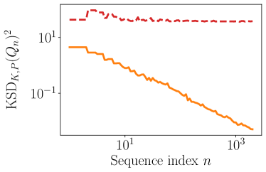
(a) Off-target sequence with non-converging means.

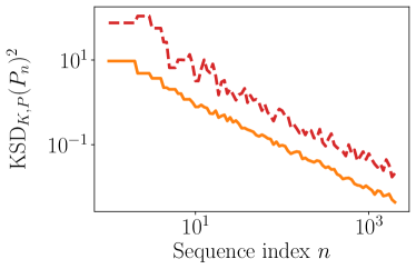
(b) On-target sequence formed by i.i.d samples from the target.

Figure 1: Importance of kernel choice for controlling first moments. (a) For a multivariate Student’s t target $P$, the standard IMQ Langevin KSD (LKSD) converges to $0$ for an off-target sequence $Q_{n}$ that does not converge to $P$ in $1$-Wasserstein distance. Meanwhile, a diffusion KSD (DKSD) with an appropriate diffusion matrix $m$ and an IMQ⁺ base kernel remains bounded away from $0$ as required by Theorem 3.9. (b) For an on-target sequence $P_{n}$ drawn i.i.d. from $P$, both KSDs decay to zero, correctly detecting the $1$-Wasserstein convergence. See Section 4.2 for more details.

Figure 1a plots the two KSDs along the off-target sequence $Q_{n}$. We can see that the LKSD decays to zero. As 3.3 suggests, since the Student’s t-distribution has a decaying score function $\nabla\log p$, the corresponding Stein RKHS cannot have a growing function with a bounded base kernel, and thus is unable to enforce first-moment uniform integrability. In contrast, the DKSD sucessfuly detects the mean non-convergence. Indeed, our choice of the diffusion matrix $m$ satisfies our assumptions and enables us to cancel the decay of the score function: as we show in aosnolinkLemma J.4, aos,arxivLemma J.4, if $\nu>2,$ the t-distribution is dissipative (Assumption 3) and $\alpha=(1-2\nu^{-1});$ in fact, it satisfies the uniform dissipativity condition in 3.17. This result confirms our theory for the DKSD, as proved in Theorem 3.9. Finally, as in the previous section, Figure 1b shows that both KSDs vanish for an on-target sample sequence $P_{n}$, demonstrating that the KSD detects the $1$-Wasserstein convergence, as 3.12 implies.

4.3 Cautionary tale: mixtures with isolated components

Our final experiment concerns the following distributions:

$$P=\frac{1}{2}{\cal N}(\mu_{1},\mathrm{Id})+\frac{1}{2}{\cal N}(\mu_{2},\mathrm{Id}),\ Q_{\pi}=\pi{\cal N}(\mu_{1},\mathrm{Id})+(1-\pi){\cal N}(\mu_{2},\mathrm{Id}),$$ (15)

where $0\leq\pi\leq 1$, $\mu_{1},\mu_{2}\in\mathbb{R}^{d}$, and ${\cal N}(\mu,\mathrm{Id})$ denotes a Gaussian distribution with mean $\mu$ and diagonal covariance $\mathrm{Id}$. The two distributions $P$ and $Q_{\pi}$ share the mixture components, with the difference arising from the variation in the mixing weight $\pi$. Varying $\pi$ shifts the mean of $Q_{\pi}$, and one might hope that the KSD will detect this discrepancy. The target $P$ is indeed supported by our theory, since Gaussian mixtures are known to be distantly dissipative (Gorham et al., 2019, Example 3). When the distance $\lVert\mu_{1}-\mu_{2}\rVert_{2}$ between the two modes is large, however, the KSD is unable to capture the discrepancy of the mixture ratio $\pi$ unless a very large sample size is observed. Figure 2 illustrates this point, using the kernel of 3.14, where $q_{m}=0$ and $q=1$. This issue has been noted by Gorham et al. (2019, Section 5.1) and Wenliang and Kanagawa (2021).

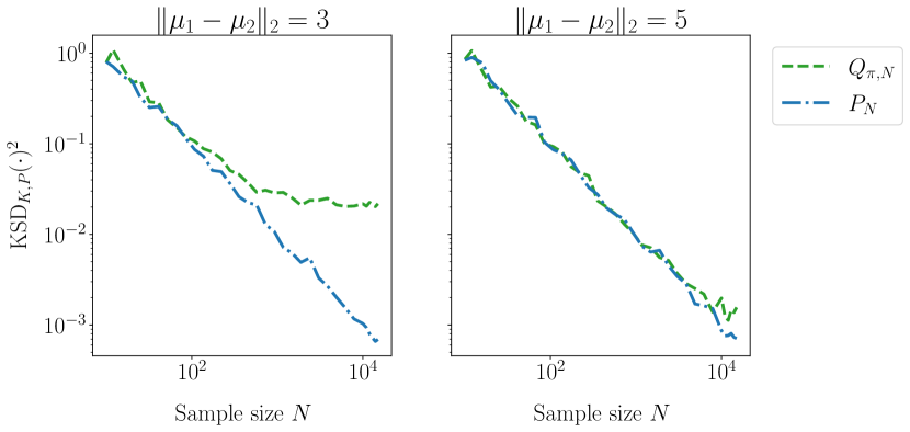
Figure 2: Impact of isolated modes on non-convergence detection. For a two-component multivariate Gaussian mixture $P$ with mode separation $\lVert\mu_{1}-\mu_{2}\rVert_{2}$, we compare the IMQ⁺ KSD of an on-target sequence $P_{N}$ drawn i.i.d. from $P$ and an off-target sequence $Q_{\pi,N}$ drawn i.i.d. from a distribution that undersamples mode $1$. The larger the mode separation $\lVert\mu_{1}-\mu_{2}\rVert_{2},$ the larger the sample size required to distinguish the on- and off-target sequences. See Section 4.3 for more details.

The insensitivity can be in part attributed to the RKHS’s lack of adaptivity to the sample. We first examine this claim using fixed kernels, as in the experiment from Figure 2. To this end, we consider the Langevin KSD with the base kernel of the form of 3.7, where $L=L^{(2)}$ in Theorem 3.9, $q_{m}=0$, and $q=1$; this choice ensures that the Stein RKHS has a function of linear growth. We study two choices of the translation invariant kernel $\ell$ : the IMQ kernel $k_{\textup{IMQ}}(x,x^{\prime})=\bigl{(}1+\lVert x-x^{\prime}\rVert_{2}^{2}/\sigma^{2}\bigr{)}^{-1/2}$ and the following Matérn kernel

$$k_{\mathrm{Mat}}(x,x^{\prime})=\left(1+\frac{\sqrt{3}\lVert x-x^{\prime}\rVert_{2}}{\sigma}\right)\exp\left(-\frac{\sqrt{3}}{\sigma}\lVert x-x^{\prime}\rVert_{2}\right).$$

As in 3.14, we term these two kernel choices IMQ⁺ and Mat⁺, respectively. Here, to capture a sensible scale, we set the bandwidth $\sigma$ equal to the median (Euclidean) distance calculated from samples drawn from the target distribution $P$.

In this setting, we use an independent sample $\{X_{i}\}_{i=1}^{N}$ from $Q_{\pi}$ to form a sequence of empirical distributions $Q_{\pi,N}=N^{-1}\sum_{i\leq N}\delta_{X_{i}}$ and exactly compute the KSD between $P$ and $Q_{\pi,N}.$ In the following, we set $\mu_{1}=-30\cdot\mathbf{1},$ $\mu_{2}=-10\cdot\mathbf{1}$ and $d=5.$ With $N$ fixed at $500,$ we vary the mixture ratio $\pi$ from $0$ to $1/2$ using a regular grid of size $30.$ We noticed that the KSD’s trajectory has different trends depending on the drawn samples. We therefore repeat this procedure 100 times and provide a summary.

Figure 3a presents density estimates of the distribution of KSD values computed from different sample draws, plotted against the mixture ratio. We observe that for both kernels, their KSDs do not change along the sequence.

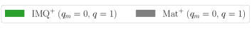
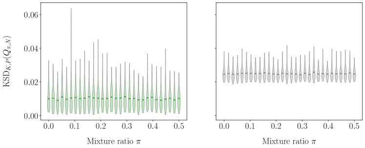
(a) KSDs with fixed length scale base kernels suffer from an insensitivity to changes in the Gaussian mixture proportion $\pi$.

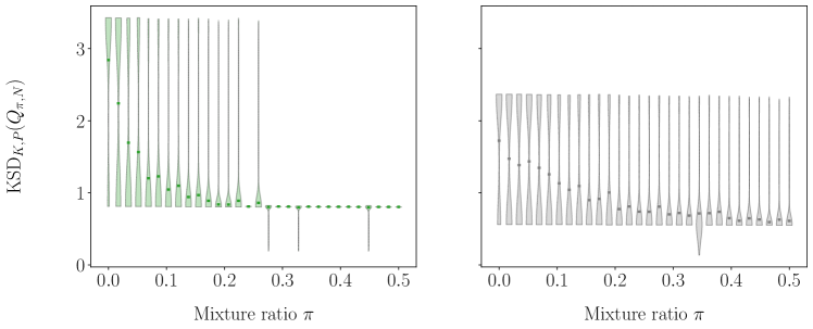
(b) KSDs with optimized length scale enjoy improved sensitivity to changes in the Gaussian mixture proportion $\pi$.

Figure 3: Impact of kernel length scale on detecting undersampled mixture components. To assess the impact of adaptively selecting the length scale of the KSD base kernel, we plot both the distribution of KSD values and their mean value (as a bold dot) over independent samples of $N=500$ points drawn i.i.d. from the Gaussian mixture $Q_{\pi}$ in Equation 15 when the target $P=Q_{1/2}$. See Section 4.3 for more details.

One can hope to improve this sensitivity by adjusting the length scale $\sigma$ adaptively. Here, following the approaches in hypothesis testing (Gretton et al., 2012b; Sutherland et al., 2016; Jitkrittum et al., 2016, 2017), we consider choosing a bandwidth by optimizing the objective $\mathrm{KSD}_{K,P}(Q_{\pi,N})^{2}/\sqrt{v_{H_{1}}},$ where $v_{H_{1}}=\mathrm{Var}_{X\sim Q_{\pi,N}}\bigl{[}\mathbb{E}_{X^{\prime}\sim Q_{\pi,N}}[k_{p,K}(X,X^{\prime})]\bigr{]}.$ This objective is a known proxy for the power of the goodness-of-fit test based on a KSD test statistic (Chwialkowski et al., 2016; Liu et al., 2016) and can be computed exactly. The optimization procedure may be interpreted as seeking a bandwidth that allows us to conclude $P\neq Q_{\pi,N}$ using as few sample points as possible, without using the whole of $Q_{\pi,N}.$ We choose a bandwidth that maximizes the objective from a regular grid between $10^{-3}$ and $10^{3}$ (in the logarithmic scale with base $10$) with the grid size $20.$

Figure 3b shows the result. Both kernels successfully manifest decreasing trends. The IMQ kernel tends to take larger values near $\pi=0,$ but stays at the same value past the point $\pi=0.3.$ In contrast, the Matérn kernel keeps the decreasing trend and captures the discrepancy. The Matérn kernel may therefore be thought of as more stable and as inducing a more stringent discrepancy measure.

5 Conclusion

In this paper, we presented necessary and sufficient conditions for the diffusion kernel Stein discrepancy to control both weak convergence and convergence of moments. These theoretical results provide guidance for choosing a reproducing kernel when applying the diffusion kernel Stein discrepancy in practice. The practical application of our results may be limited by the need to validate the assumptions on the target distribution, like that of dissipativity (Assumption 2). Developing a discrepancy measure that is adaptive to the target is desirable and left for future work.

Acknowledgements

HK was supported by the EPSRC grant [EP/W019590/1] and in part by the Gatsby Charitable Foundation. AB gratefully acknowledges funding from the Turing-Roche Strategic Partnership. AG acknowledges financial support by the Gatsby Charitable Foundation. The authors thank Chris Oates for his helpful feedback, and Carl-Johann Simon-Gabriel for the constructive discussions.

Appendix A Proof of Proposition 3.3:
Standard KSDs fail to control moments

This appendix presents a proof of 3.3. We provide a result that holds for a more general maximum mean discrepancy [MMD, Gretton et al., 2012a]. The claim for the KSD follows once we address the MMD case, since the KSD is an specific instance of the MMD (see Section 2).

Recall that for a scalar-valued kernel, the MMD is defined as an IPM (see Eq. 4 for the definition): $\mathrm{MMD}_{k}(P,Q)=d_{\mathcal{B}_{k}}(P,Q)$, where $\mathcal{B}_{k}$ is the unit ball $\{h\in\mathcal{H}_{k}:\lVert h\rVert_{\mathcal{H}_{k}}\leq 1\}$ of the RKHS $\mathcal{H}_{k}$. If $\mathcal{H}_{k}\subset L^{1}(P)\cap L^{1}(Q)$, we have

$$\mathrm{MMD}_{k}(P,Q)^{2}=\int\int k(x,y)\differential\bigl{(}P-Q\bigr{)}(x)\differential\bigl{(}P-Q\bigr{)}(y).$$

For a finite signed measure $\mu$ such that $\mathcal{H}_{k}\subset L^{1}(\lvert\mu\rvert)$, we also denote

$$\lVert\mu\rVert_{k}\coloneqq\sqrt{\int\int k(x,y)\differential\mu(x)\differential\mu(y)}$$

so that $\mathrm{MMD}_{k}(P,Q)=\lVert P-Q\rVert_{k}$.

Here, we generalize our setup to a metric space $(\mathcal{X},d)$, and consider $q$-Wasserstein convergence accordingly:

Definition A.1 ($q$-Wasserstein convergence in metric spaces).

Let $({\cal X},d)$ be a separable metric space. We define the set of Borel probability measures with finite $q$th moments by

$${\cal P}_{q}({\cal X})=\left\{\mu:\int d(x,\bar{x})^{q}\differential\mu(x)<\infty\ \text{for some}\ \bar{x}\in{\cal X}\right\}.$$

A function $f:{\cal X}\to\mathbb{R}$ is said to be of $q$-growth if there exists a constant $C>0$ such that

$$f(x)\leq C(1+d(x,x_{0})^{q})$$

for some (and then any) $x_{0}\in{\cal X}.$ A sequence $\{P_{n}\}_{n\geq 1}\subset{\cal P}_{q}({\cal X})$ is said to converge to $P$ in $q$-Wasserstein convergence if

$$\int f\differential P_{n}\to\int f\differential P$$

for any continuous function $f$ of $q$-growth.

We are ready to provide the result. The following proposition demonstrates that the MMD cannot detect moment non-convergence when its RKHS lacks $q$-growth functions.

Proposition A.2 ($q$-growth is necessary for enforcing $q$th moment convergence).

Let $(\mathcal{X},d)$ be an unbounded separable metric space. Let $q\in(0,\infty)$ and $P\in{\cal P}_{q}(\mathcal{X})$. Let $k:\mathcal{X}\times\mathcal{X}\to\mathbb{R}$ be a kernel satisfying the following growth condition: there exist some $C,R>0$ and some $x_{0}$ such that

$$\sqrt{k(x,x)}\leq C\{1+d(x_{0},x)^{q^{\prime}}\}$$

for all $x\in\mathcal{X}$ with $d(x,x_{0})>R$, where $0<q^{\prime}<q$. Then, vanishing $\mathrm{MMD}_{k}(P,\cdot)$ does not imply $q$-Wasserstein convergence to $P$.

3.3 follows as a corollary of this proposition. Note that under Assumption 1, from the expression of the Stein kernel (Eq. 29), we have $\sqrt{k_{p,K}(x,x)}\leq C(1+\lVert x\rVert_{2})$ for some constant $C>0$. As a result, for $q>1$, the KSD cannot control $q$-Wasserstein convergence. We provide a proof as follows.

Proof.

We construct a sequence in ${\cal P}_{q}(\mathcal{X})$ that converges to $P$ in MMD but not in $q$-Wasserstein convergence. Let $n\geq 1$ be an integer such that there exists a point $x_{n}\in\mathcal{X}$ with $(n-1)^{1/q}\leq d(x_{0},x_{n})\leq n^{1/q}$. There are infinitely many such $n$ as $\mathcal{X}$ is bounded otherwise. Let $\{n(j)\}_{j\geq 1}$ be a sequence of such integers with $x_{j}$ the corresponding point. Then, define a sequence

$$Q_{j}=\left(1-\frac{1}{n(j)+1}\right)P+\frac{1}{n(j)+1}\delta_{x_{j}}.$$

For $j\geq 1$ with $d(x_{j},x_{0})>R$, we have

$$\mathrm{MMD}_{k}(P,Q_{j}) \leq\frac{1}{n(j)+1}\lVert P\rVert_{k}+\frac{1}{n(j)+1}\lVert\delta_{x_{j}}\rVert_{k}$$

$$=\frac{1}{n(j)+1}\lVert P\rVert_{k}+\frac{1}{n(j)+1}\sqrt{k(x_{j},x_{j})}$$

$$\leq\frac{1}{n(j)+1}\lVert P\rVert_{k}+\frac{C}{n(j)+1}\left(1+n(j)^{q^{\prime}/q}\right)\to 0\ (j\to\infty).$$

Thus, $Q_{j}$ converges to $P$ in MMD. On the other hand, for any continuous bounded function $f$,

$$\int f\differential Q_{j} =\left(1-\frac{1}{n(j)+1}\right)\int f\differential P+\underbrace{\frac{1}{n(j)+1}f(x_{j})}_{\to 0}$$

$$\to\int f\differential P\ (j\to\infty),$$

where we have used the boundedness of $f$ to diminish the second term in the limit. Hence, $Q_{j}$ weakly converges to $P$. Moreover, we have

$$\int d(x_{0},\cdot)^{q}\differential Q_{j} =\left(1-\frac{1}{n(j)+1}\right)\int d(x_{0},\cdot)^{q}\differential P+\frac{1}{n(j)+1}d(x_{0},x_{j})^{q}$$

$$\geq\left(1-\frac{1}{n(j)+1}\right)\int d(x_{0},\cdot)^{q}\differential P+\frac{n(j)-1}{n(j)+1}.$$

Taking the limit on both sides implies that $Q_{j}$ does not converge to $P$ in the $q$th moment. Thus, we have constructed the desired sequence, and the proof is complete. ∎

Appendix B Approximating $q$-growth

In this appendix, it is shown that we can construct a Stein RKHS $\mathcal{T}_{P}^{m}(\mathcal{H}_{K})$ that approximates $q$-growth. Our strategy is as follows. First, we construct a vector-valued function $v_{\varepsilon}$ such that $\mathcal{T}_{P}^{m}v_{\varepsilon}$ approximates $q$-growth up to precition $\varepsilon$, i.e., $\mathcal{T}_{P}^{m}v_{\varepsilon}$ satisfies

$$\mathcal{T}_{P}^{m}v_{\varepsilon}(x)\geq\lVert x\rVert_{2}^{q}1\{\lVert x\rVert_{2}>r_{\varepsilon}\}-\varepsilon$$

for some ${r_{\varepsilon}}>0$ — Lemma B.1 serves this purpose. Note that $v_{\epsilon}$ may not be belong to the RKHS. Thus, we approximate it using a function of the RKHS; we provide two such results in Section B.2.

B.1 Preparatory results

Lemma B.1 (Existence of $q$-growth approximation).

For $r,\delta>0,$ define a $\mathcal{C}^{2}$-function $1_{r,\delta}(x)=h_{r,\delta}(\lVert x\rVert_{2})$ with

$$h_{r,\delta}(t)=\frac{f(r+\delta-t)}{f(r+\delta-t)+f(t-r)}$$

and $f(t)=t^{3}1_{[0,\infty)}(t)$, $t\in\mathbb{R}$. Let $q\in[0,\infty).$ Assume the dissipativity condition in Assumption 2 with $\alpha,\beta_{1},\beta_{0}.$ Suppose Assumption 1 holds for some constants $c_{m}>0$ and $q_{m}\in\{0,1\}$; if $q_{m}=1,$ additionally assume $\alpha>\lambda_{m}(q+2).$ Then, for any $\varepsilon>0,$ there exist positive constants $r,\delta,\eta$ such that

$$\mathcal{T}_{P}^{m}(\tilde{1}_{r,\delta}v)(x)\geq\eta\lVert x\rVert_{2}^{q}1\{\lVert x\rVert_{2}\geq r+\delta\}-\varepsilon 1\{r<\lVert x\rVert_{2}<r+\delta\}$$

where $\tilde{1}_{r,\delta}=1-1_{r,\delta},$ $v(x)=-\tilde{w}(x)x$ with $\tilde{w}(x)=\bigl{(}\tau^{2}+\lVert x\rVert_{2}^{2}\bigr{)}^{\frac{q}{2}-1};$ and the constant $\eta$ is determined by the following quantities: $\alpha,$ $\beta_{1},$ $\beta_{0},$ $\lambda_{m},$ $\tau,$ $q_{m},$ and $q.$ In particular, we may take $r+\delta\geq 1$ .

Proof.

Given positive constants $r,\delta,$ our proof separately considers the three regimes: $\lVert x\rVert_{2}\leq r,$ $r<\lVert x\rVert_{2}<r+\delta,$ and $\lVert x\rVert_{2}\geq r+\delta.$ We then choose suitable $r,\delta.$

First, if $\lVert x\rVert_{2}\leq r,$ we have $\tilde{1}_{r,\delta}(x)=0$ and thus $\mathcal{T}_{P}^{m}(\tilde{1}_{r,\delta}v)(x)=0,$ for any choice of $r$ and any $v$ in the domain of $\mathcal{T}_{P}^{m}.$ In the following, we consider $v(x)=-\tilde{w}(x)x$ as claimed.

In the regime $r<\lVert x\rVert_{2}<r+\delta,$ we show that for any $\varepsilon>0,$ we can choose $r,\delta>0$ such that $\mathcal{T}_{P}^{m}(\tilde{1}_{r,\delta}v)(x)\geq-\varepsilon.$ With $\lVert x\rVert_{2}=t$ and $\tilde{h}_{r,\delta}(t)=1-h_{r,\delta}(t)$, we have

$$\mathcal{T}_{P}^{m}(\tilde{1}_{r,\delta}v)(x)$$

$$=\tilde{1}_{r,\delta}(x){\cal T}_{P}^{m}v(x)-h_{r,\delta}^{{}^{\prime}}\bigl{(}\lVert x\rVert_{2}\bigr{)}\langle m(x),x\otimes v(x)\rangle\frac{1}{\lVert x\rVert_{2}}$$

$$=\tilde{w}(t)\tilde{h}_{r,\delta}(t)\left\{-\mathcal{T}_{P}^{m}x-\frac{2(q/2-1)t^{2}}{\tau^{2}+t^{2}}\frac{\left\langle m(x),x\otimes x\right\rangle}{t^{2}}\right.$$

$$\hphantom{=\tilde{w}(t)\bigl{(}1-h_{r,\delta}(t)\bigr{)}}\quad\left.-\frac{h^{\prime}_{r,\delta}(t)}{\tilde{h}_{r,\delta}(t)}\frac{\left\langle m(x),x\otimes x\right\rangle}{t^{2}}t\right\}$$

$$\geq\tilde{w}(t)\tilde{h}_{r,\delta}(t)\left[\alpha t^{2}-\beta_{1}t-\beta_{0}-\lambda_{m}\left(q-2+\frac{h^{\prime}_{r,\delta}(t)}{\tilde{h}_{r,\delta}(t)}t\right)(c_{m}+t^{q_{m}+1})\right]$$

$$=\begin{aligned} \tilde{w}(t)\left[\tilde{h}_{r,\delta}(t)\cdot\left\{\alpha t^{2}-\beta_{1}t-\beta_{0}-\lambda_{m}\left(q-2+\omega_{r,\delta}(t)\right)(c_{m}+t^{q_{m}+1})\right\}\right.\\ \hphantom{=\tilde{w}(t)}\quad\left.-\lambda_{m}r\cdot h^{\prime}_{r,\delta}(t)(c_{m}+t^{q_{m}+1})\right]\end{aligned}$$

$$\geq\begin{aligned} \tilde{w}(t)\left[\frac{(t-r)^{3}}{(r+\delta-t)^{3}+(t-r)^{3}}\cdot\left\{\alpha t^{2}-\beta_{1}t-\beta_{0}-\lambda_{m}(q+2)(c_{m}+t^{q_{m}+1})\right\}\right.\\ \hphantom{=\tilde{w}(t)}\quad\left.-\lambda_{m}r\frac{3\delta(r+\delta-t)^{2}(t-r)^{2}}{\{(r+\delta-t)^{3}+(t-r)^{3}\}^{2}}(c_{m}+t^{q_{m}+1})\right]\end{aligned}$$ (16)

where $\tilde{w}(t)=\bigl{(}\tau^{2}+t^{2}\bigr{)}^{q/2-1}$ and $\omega_{r,\delta}(t)\coloneqq 3\delta(r+\delta-t)^{2}/\{(r+\delta-t)^{3}+(t-r)^{3}\}$; the first inequality is derived from the dissipativity (Assumption 2) and the growth condition on $\lVert m(x)\rVert_{\mathrm{op}}$ (Assumption 1); to obtain the second inequality, we have used $\omega_{r,\delta}(t)\leq 4$ for $r<t<r+\delta$. In the lower bound (16), we have a quadratic function inside the braces in the first term, where, by assumption, the quadratic term has positive coefficients $\alpha$ and $\alpha-\lambda_{m}(q+2)$ for $q_{m}=0$ and $q_{m}=1,$ respectively. Thus, by choosing $r>0$ (independent of $\delta)$ appropriately, we can make this quadratic function both positive and increasing in the interval $(r,r+\delta).$ We denote this value of $r$ by $r_{0}.$

The lower bound (16) may become negative, but we show that its magnitude can be made arbitrarily small by choosing $r$ and $\delta$ judiciously. To see this, note that the second term of (16) dominates the first iff

$$\frac{\alpha}{3\lambda_{m}}\frac{\theta(1+\theta^{3})}{(1+\theta)^{2}}\frac{\delta}{r}\cdot\frac{t^{2}-\lambda_{m}(q+2)/\alpha\cdot t^{q_{m}+1}-(\beta_{1}/\alpha)t-\beta_{0}/\alpha-\lambda_{m}c_{m}(q+2)/\alpha}{t^{q_{m}+1}+c_{a}}\leq 1,$$ (17)

where $\theta=(t-r)/(r+\delta-t)\in(0,\infty).$ By taking sufficiently large $r,$ we may assume that for any $t>r,$

$$\frac{t^{q_{m}+1}+c_{m}}{t^{2}-\lambda_{m}(q+2)/\alpha\cdot t^{q_{m}+1}-(\beta_{1}/\alpha)t-\beta_{0}/\alpha-\lambda_{m}c_{m}(q+2)/\alpha}\leq C$$

for some constant $C>0.$ If $q_{m}=0,$ we may choose any $C>0,$ whereas if $q_{m}=1,$ we need $C>\{1-\lambda_{m}(q+2)/\alpha\}^{-1}.$ Indeed, such $r$ can be chosen by examining the following conditions:

$$\begin{cases}0\leq Ct^{2}-\bigl{[}C\bigl{\{}\frac{\beta_{1}}{\alpha}+\lambda_{m}\frac{q+2}{\alpha}\bigr{\}}+1\bigr{]}t-C\left\{\frac{\beta_{0}}{\alpha}+\frac{\lambda_{m}c_{m}(q+2)}{\alpha}+\frac{c_{m}}{C}\right\}&\text{if }q_{m}=0,\\ 0\leq\bigl{[}C\{1-\frac{\lambda_{m}(q+2)}{\alpha}\}-1\bigr{]}t^{2}-C\frac{\beta_{1}}{\alpha}t-C\left\{\frac{\beta_{0}}{\alpha}+\frac{\lambda_{m}c_{m}(q+2)}{\alpha}+\frac{c_{m}}{C}\right\}&\text{if }q_{m}=1.\end{cases}$$

Let $r_{1}$ be a value of such $r.$ Using $r=r_{0}\lor r_{1},$ the inequality (17) implies

$$\frac{\theta(1+\theta^{3})}{(1+\theta)^{2}}\leq\frac{3\lambda_{m}C}{\alpha}\frac{r}{\delta}.$$ (18)

Then, the magnitude of the second term is evaluated as follows: we have

$$\tilde{w}(t)=\left\{\tau^{2}+\left(\frac{\theta(1+\theta^{3})}{(1+\theta)^{2}}\frac{1+\theta}{1+\theta^{3}}\delta+r\right)^{2}\right\}^{q/2-1}$$

$$\leq\begin{cases}\frac{1}{\tau^{q-2}}&q\leq 2\\ \left\{\tau^{2}+\left(\frac{4\lambda_{m}C}{\alpha}+1\right)^{2}r^{2}\right\}^{q/2-1}&q>2\end{cases},$$

and

$$3\lambda_{m}r\delta\frac{(r+\delta-t)^{2}(t-r)^{2}}{\{(r+\delta-t)^{3}+(t-r)^{3}\}^{2}}(c_{m}+t^{q_{m}+1})$$

$$=3\lambda_{m}\frac{\theta^{2}}{(1+\theta)^{4}}\frac{(1+\theta)^{6}}{(1+\theta^{3}){}^{2}}\left\{c_{m}+\left(\frac{\theta}{1+\theta}\delta+r\right)^{q_{m}+1}\right\}\frac{r}{\delta}$$

$$=3\lambda_{m}\left(\frac{\theta(1+\theta^{3})}{(1+\theta)^{2}}\right)^{2}\frac{(1+\theta)^{6}}{(1+\theta^{3}){}^{4}}\left\{c_{m}+\left(\frac{1+\theta}{1+\theta^{3}}\frac{\theta(1+\theta^{3})}{(1+\theta)^{2}}\delta+r\right)^{q_{m}+1}\right\}\frac{r}{\delta}$$

$$\overset{\text{\eqref{eq:norm-indicator-theta-eval}}}{\leq}\frac{27\lambda_{m}^{3}C^{2}}{\alpha^{2}}\left(\frac{123+55\sqrt{5}}{32}\right)\left\{c_{m}+\left(\frac{4\lambda_{m}C}{\alpha}+1\right)^{q_{m}+1}r^{q_{m}+1}\right\}\cdot\left(\frac{r}{\delta}\right)^{3}.$$ (19)

The product of these provides the desired estimate of the magnitude. For a given $r,$ as $\delta$ grows, the evaluation (19) decays at the rate of $\delta^{-3}.$ Hence, for any $\varepsilon>0,$ we can choose sufficiently large $\delta$ such that the domination by the second term in (16) is at most by $\varepsilon;$ i.e., $\mathcal{T}_{P}^{m}\bigl{(}\tilde{1}_{r,\delta}v\bigr{)}(x)\geq-\varepsilon$ for $r<\lVert x\rVert_{2}<r+\delta.$ We denote such choice of $\delta$ by $\delta_{\varepsilon}(r).$

Finally, consider the regime $\lVert x\rVert_{2}\geq r+\delta,$ where $\mathcal{T}_{P}^{m}(\tilde{1}_{r,\delta}v)(x)=\mathcal{T}_{P}^{m}v(x).$ We show that a suitable value of $r+\delta$ yields $\mathcal{T}_{P}^{m}v(x)\geq\eta\lVert x\rVert_{2}^{q}$ for some $\eta>0.$ By Assumption 2 and the growth condition on $\lVert m(x)\rVert_{\mathrm{op}},$ we have

$$\mathcal{T}_{P}^{m}v(x) \geq\tilde{w}(\lVert x\rVert_{2})\left(\alpha\lVert x\rVert_{2}^{2}-\beta_{1}\lVert x\rVert_{2}-\beta_{0}-\lambda_{m}(q-2)\frac{\lVert x\rVert_{2}^{2}}{(\tau^{2}+\lVert x\rVert_{2}^{2})}\bigl{(}c_{m}+\lVert x\rVert_{2}^{q_{m}+1}\bigr{)}\right)$$

$$\geq\tilde{f}\bigl{(}\lVert x\rVert_{2}\bigr{)}\left(1+\frac{\tau^{2}}{\lVert x\rVert_{2}^{2}}\right)^{\frac{q}{2}-1}\lVert x\rVert_{2}^{q},$$

where

$$\tilde{f}(t)=\left\{\alpha-\frac{1}{t^{2}}\left(\beta_{1}t+\beta_{0}+\lambda_{m}(q-2)\bigl{(}c_{m}+t^{q_{m}+1}\bigr{)}1\{q>2\}\right)\right\}.$$

Due to the monotonicity of $\tilde{f},$ we have $\delta_{0}$ such that $\tilde{f}(\delta_{0})=0.$ By the requirement on $r_{0},$ it turns out $r_{0}>\delta_{0}.$ Therefore, if $q\geq 2,$ we have ${\cal T}_{P}g(x)\geq\eta\lVert x\rVert_{2}^{q}$ for $\lVert x\rVert_{2}\geq r_{0}$ and $\eta=\tilde{f}(r_{0});$ if $q<2,$ we have $\mathcal{T}_{P}^{m}g(x)\geq\eta\lVert x\rVert^{q}$ for $\lVert x\rVert_{2}\geq r_{0}\lor\tau^{2}\bigl{(}2^{2/\lvert q-2\rvert}-1\bigr{)}^{-1}$ and $\eta=2^{-1}\text{$\tilde{f}(r_{0})$}.$

The consideration for the above three regimes of $\lVert x\rVert_{2}$ suggests that we should choose $\delta=\delta_{\varepsilon}(r),$ and $r=r_{0}\lor r_{1}$ if $q\geq 2,$ and $r=r_{0}\lor r_{1}\lor\tau^{2}\bigl{(}2^{2/\lvert q-2\rvert}-1\bigr{)}^{-1},$ otherwise. This choice yields

$$\mathcal{T}_{P}^{m}\bigl{(}\tilde{1}_{r,\delta}v\bigr{)}(x) \geq\eta\lVert x\rVert_{2}^{q}1\{\lVert x\rVert_{2}\geq r+\delta\}-\varepsilon 1\{r<\lVert x\rVert_{2}<r+\delta\}$$

for any $x\in\mathbb{R}^{d}.$ ∎

Corollary B.2 (Concrete choices of $r$ and $\delta$ in Lemma B.1).

Lemma B.1 holds for

$$r =\begin{cases}r_{1}&q\geq 2\\ r_{1}\lor\tau^{2}\bigl{(}2^{2/\lvert q-2\rvert}-1\bigr{)}^{-1}&0\leq q<2\end{cases}$$

$$\delta =W_{r}r\cdot\varepsilon^{-\frac{1}{3}},$$

where

$$r_{1}=\begin{cases}\frac{\{\beta_{1}+\lambda_{m}(q+2)\}+1+\sqrt{[\{\beta_{1}+\lambda_{m}(q+2)\}+1]^{2}+4\alpha\left\{\beta_{0}+\lambda_{m}c_{a}(q+2)+c_{m}\right\}}}{2\alpha}&q_{m}=0\\ \frac{2\beta_{1}+2\sqrt{\beta_{1}^{2}+2\tilde{\alpha}\{\lambda_{m}c_{m}(q+2)+\beta_{0}\}+\tilde{\alpha}c_{m}}}{2\tilde{\alpha}}&q_{m}=1,\end{cases}$$

$$W_{r}^{3}=$$

$$\begin{cases}\bigl{(}\tau^{-(q-2)}\lor\bar{w}_{0}(r)\bigr{)}27\lambda_{m}^{3}\left(\frac{123+55\sqrt{5}}{32}\right)\left\{c_{m}+\left(4\lambda_{m}+1\right)r\right\}&q_{m}=0\\ \bigl{(}\tau^{-(q-2)}\lor\bar{w}_{1}(r)\bigr{)}\frac{4\cdot 27\lambda_{m}}{\{\alpha-\lambda_{m}(q+2)\}^{2}}\left(\frac{123+55\sqrt{5}}{32}\right)\left\{c_{m}+\left(\frac{8\lambda_{m}}{\alpha-\lambda_{m}(q+2)}+1\right)^{2}r^{2}\right\}&q_{m}=1,\end{cases}$$

$\bar{w}_{0}(r)=\{\tau^{2}+\left(4\lambda_{m}+1\right)^{2}r^{2}\}^{q/2-1},$ and $\bar{w}_{1}(r)=\bigl{[}\tau^{2}+\bigl{\{}2\lambda_{m}/\bigl{(}\alpha-\lambda_{m}(q+2)\bigr{)}+1^{2}\bigr{\}}r^{2}\bigr{]}^{q/2-1}.$ Thus, $r+\delta=(1+W_{r}\varepsilon^{-\frac{1}{3}})r.$ In particular, we may take $r\geq 1$ to ensure $r+\delta>1.$

Proof.

We follow the notation in the proof of Lemma B.1. We consider the two cases $q_{m}=0$ and $q_{m}=1$ separately.

We first examine the case $q_{m}=0.$ Here, by checking the requirement on $r_{0},$ we obtain

$$r_{0} =\frac{\beta_{1}+\lambda_{m}(q+2)+\sqrt{\left(\beta_{1}+\lambda_{m}(q+2)\right)^{2}+4\alpha\left(\lambda_{m}c_{m}(q+2)+\beta_{0}\right)}}{2\alpha}$$

and with $C=\alpha$ in the proof of Lemma B.1, the condition on $r_{1}$ implies

$$r_{1} =\frac{\{\beta_{1}+\lambda_{m}(q+2)\}+1+\sqrt{[\{\beta_{1}+\lambda_{m}(q+2)\}+1]^{2}+4\alpha\left\{\beta_{0}+\lambda_{m}c_{a}(q+2)+c_{m}\right\}}}{2\alpha}>r_{0}.$$

We then obtain $\delta_{\varepsilon}(r)=W_{r}r\varepsilon^{-1/3}$ with

$$W_{r}^{3}=\bar{w}(r)\cdot 27\lambda_{m}^{3}\left(\frac{123+55\sqrt{5}}{32}\right)\left\{c_{m}+\left(4\lambda_{m}+1\right)r\right\}$$

and $\bar{w}(r)=\left\{\tau^{2}+\left(4\lambda_{m}+1\right)^{2}r^{2}\right\}^{q/2-1}\lor\tau^{-(q-2)}.$

Next, we similarly investigate the case $q_{m}=1.$ With $\tilde{\alpha}=\alpha-\lambda_{m}(q+2),$ we have

$$r_{0}=\frac{\beta_{1}+\sqrt{\beta_{1}^{2}+4\tilde{\alpha}\{\lambda_{m}c_{m}(q+2)+\beta_{0}\}}}{2\tilde{\alpha}}$$

and by choosing $C=2\alpha(\tilde{\alpha})^{-1},$ we obtain

$$r_{1} =\frac{2\beta_{1}+2\sqrt{\beta_{1}^{2}+2\tilde{\alpha}\{\lambda_{m}c_{m}(q+2)+\beta_{0}\}+\tilde{\alpha}c_{m}}}{2\tilde{\alpha}}$$

$$>r_{0}$$

Thus, $\delta_{\varepsilon}=W_{r}r\varepsilon^{-\frac{1}{3}}$ with

$$W_{r}^{3}=\bar{w}(r)\frac{4\cdot 27\lambda_{m}^{3}}{\{\alpha-\lambda_{m}(q+2)\}^{2}}\left(\frac{123+55\sqrt{5}}{32}\right)\left\{c_{m}+\left(\frac{8\lambda_{m}}{\alpha-\lambda_{m}(q+2)}+1\right)^{2}r^{2}\right\}$$

and

$$\bar{w}(r)=\left\{\tau^{2}+\left(\frac{8\lambda_{m}}{\alpha-\lambda_{m}(q+2)}+1\right)^{2}r^{2}\right\}^{q/2-1}\lor\tau^{-(q-2)}.$$

∎

B.2 Proof of Lemma 3.8: (Kernel choice for $q$-growth approximation).

Lemma B.1 provides a concrete function to approximate $q$-growth. To prove Lemma 3.8, we approximate this function using an RKHS function. Our proof is divided into two parts: the first proof deals with the general universal kernel, while the second proof deals with the translation-invariant kernel case (see Corollary B.6).

B.2.1 Proof via universality

Lemma B.3 (Stein RKHS with universal kernel approximates $q$-growth).

Let $q\in[0,\infty).$ Let $K:\mathbb{R}^{d}\times\mathbb{R}^{d}\to\mathbb{R}^{d\times d}$ be a matrix-valued kernel defined by

$$K(x,y)=w(x)w(y)\left(L(x,y)+\bar{k}_{\mathrm{lin}}(x,y)\mathrm{Id}\right),$$

where $w(x)=\bigl{(}\tau^{2}+\lVert x\rVert_{2}^{2}\bigr{)}^{(q-1)/2}$ with $\tau>0;$ $L$ is universal $\mathcal{C}_{0}^{1}\bigl{(}\mathbb{R}^{d}\bigr{)};$ and

$$\bar{k}_{\mathrm{lin}}(x,y)=\frac{\tau^{2}+\langle x,y\rangle}{\sqrt{\tau^{2}+\lVert x\rVert_{2}^{2}}\sqrt{\tau^{2}+\lVert y\rVert_{2}^{2}}}.$$

Then, under the same assumptions as in Lemma B.1, ${\cal T}_{P}^{m}(\mathcal{H}_{K})$ approximates $q$-growth.

Proof.

Let $v(x)=-w(x)x/\sqrt{\tau^{2}+\lVert x\rVert_{2}^{2}}.$ For any $\varepsilon>0,$ by Lemma B.1, there exist positive constants $r,\delta,\eta$ such that

$$\mathcal{T}_{P}\bigl{(}v-1_{r,\delta}v\bigr{)}(x)\geq\eta\lVert x\rVert_{2}^{q}1\{\lVert x\rVert_{2}\geq r+\delta\}-\frac{\eta\varepsilon}{4}1\{r<\lVert x\rVert_{2}<r+\delta\}$$ (20)

where $r+\delta\geq 1,$ and $1_{r,\delta}\in\mathcal{C}^{2}$ is a function defined in Lemma B.1) satisfying $1_{r,\delta}(x)=1$ if $\lVert x\rVert_{2}\leq r+\delta,$ $1_{r,\delta}(x)=0$ if $\lVert x\rVert_{2}\geq r+\delta,$ and $0<1_{r,\delta}(x)<1,$ otherwise. Our choice of kernel implies $v\in\mathcal{H}_{K}$, whereas $1_{r,\delta}v$ may not be an element of $\mathcal{H}_{K}.$ Thus, we approximate the latter using a function in the RKHS defined by kernel $w(x)w(y)L(x,y).$

We choose our approximation as follows. Define $\tilde{v}(x)=$$-1_{r,\delta}(x)\cdot x/\sqrt{\tau^{2}+\lVert x\rVert^{2}}$ so that $1_{r,\delta}v(x)=w(x)\tilde{v}(x).$ Since $\nabla 1_{r,\delta}(x)$ is supported in $\{\lVert x\rVert\leq r+\delta\},$$\tilde{v}$ is an element of ${\cal C}_{0}^{1}(\mathbb{R}^{d}).$ By the ${\cal C}_{0}^{1}(\mathbb{R}^{d})$-universality of the RKHS $\mathcal{H}_{L},$ for $\rho>0$ (specified below), we have an element $v_{\rho}=(v_{\rho}^{1},\dots,v_{\rho}^{d})\in\mathcal{H}_{L}$ approximating $\tilde{v}$ such that

$$\sup_{x\in\mathbb{R}^{d}}\left(\lvert v_{\rho}^{i}(x)-\tilde{v}^{i}(x)\rvert\lor\max_{j\in\{1,\dots,d\}}\lvert\partial_{x^{j}}v_{\rho}^{i}(x)-\partial_{x^{j}}\tilde{v}^{i}(x)\rvert\right)\leq\rho.$$

This in turn implies

$$\sup_{x\in\mathbb{R}^{d}}\lVert v_{\rho}(x)-\tilde{v}(x)\rVert_{2}\leq\sqrt{d}\rho\ \text{and\ }\sup_{x\in\mathbb{R}^{d}}\lVert\nabla v_{\rho}(x)-\nabla\tilde{v}(x)\rVert_{\mathrm{F}}\leq d\rho.$$ (21)

Note that we have

$$\mathcal{T}_{P}^{m}\bigl{(}v-wv_{\rho}\bigr{)}(x) =\mathcal{T}_{P}^{m}\bigl{(}v-w\tilde{v}\bigr{)}(x)+\mathcal{T}_{P}^{m}\bigl{(}w\tilde{v}-wv_{\rho}\bigr{)}(x)$$

$$\geq\eta\lVert x\rVert_{2}^{q}1\{\lVert x\rVert_{2}\geq r+\delta\}-\frac{\eta\varepsilon}{4}1\{r<\lVert x\rVert_{2}<r+\delta\}$$

$$\hphantom{\geq}\quad-\lvert\mathcal{T}_{P}^{m}\bigl{(}w\tilde{v}-wv_{\rho}\bigr{)}(x)\rvert.$$

Thus, our goal is to choose $\rho$ such that the error $\lvert\mathcal{T}_{P}^{m}\bigl{(}w\tilde{v}-wv_{\rho}\bigr{)}(x)\rvert$ grows more slowly than $\eta\lVert x\rVert_{2}^{q}$ if $\lVert x\rVert_{2}>r+\delta$ and can be made small if $\lVert x\rVert_{2}\leq r+\delta$.

We evaluate the error of $wv_{\rho}$ when applied to the Stein operator $\mathcal{T}_{P}^{m}:$

$$\left|\mathcal{T}_{P}^{m}wv_{\rho}(x)-\mathcal{T}_{P}^{m}w\tilde{v}(x)\right|$$

$$\leq\begin{aligned} &w(x)\left(2\lVert b(x)\rVert_{2}\lVert v_{\rho}(x)-\tilde{v}(x)\rVert_{2}+\lvert q-1\rvert\frac{\lVert x\rVert_{2}}{\tau^{2}+\lVert x\rVert^{2}}\lVert m(x)\rVert_{\mathrm{op}}\lVert v_{\rho}(x)-\tilde{v}(x)\rVert_{2}\right.\\ &\hphantom{w(x)}\left.\quad+\text{$\sqrt{d}$}\lVert m(x)\rVert_{\mathrm{op}}\lVert\nabla v_{\rho}(x)-\nabla\tilde{v}(x)\rVert_{\mathrm{F}}\right)\end{aligned}$$ (22)

We bound the estimate (22) to prove the statement for $q_{m}=0.$

Using the universality properties (21), we can evaluate (22) as

$$\lvert{\cal T}_{P}wv_{\rho}(x)-{\cal T}_{P}w\tilde{v}(x)\rvert$$

$$\leq\sqrt{d}\rho\cdot w(x)\left(2\lVert b(x)\rVert_{2}+\frac{\lVert x\rVert_{2}}{\tau^{2}+\lVert x\rVert^{2}}\lvert q-1\rvert\lVert m(x)\rVert_{\mathrm{op}}+d\lVert m(x)\rVert_{\mathrm{op}}\right)$$

$$\leq\rho\cdot w(x)\pi(\lVert x\rVert_{2}),$$

where we have defined $\pi$ by

$$\pi(\lVert x\rVert_{2}) \coloneqq\sqrt{d}\left\{2\lambda_{b}\bigl{(}1+\lVert x\rVert_{2}\bigr{)}+\lambda_{m}\frac{\lVert x\rVert_{2}}{\tau^{2}+\lVert x\rVert^{2}}(q-1)_{+}\bigl{(}c_{m}+\lVert x\rVert_{2}\bigr{)}+\lambda_{m}d\bigl{(}c_{m}+\lVert x\rVert_{2}\bigr{)}\right\}$$

$$\leq\sqrt{d}\left\{2\lambda_{b}\bigl{(}1+\lVert x\rVert_{2}\bigr{)}+\lambda_{m}(q-1)_{+}\bigl{(}c_{m}\tau^{-2}+1\bigr{)}+\lambda_{m}d\bigl{(}c_{m}+\lVert x\rVert_{2}\bigr{)}\right\}$$

The function $\pi$ satisfies $w(x)\pi\bigl{(}\lVert x\rVert_{2}\bigr{)}<C\lVert x\rVert_{2}^{q}$ with

$$C=\bigl{(}1+\tau^{2}\bigr{)}^{q/2}\left[2\lambda_{b}+\lambda_{m}d+\left\{2\lambda_{b}+\lambda_{m}(q-1)_{+}\left(c_{m}\tau^{-2}+1\right)+\lambda_{m}c_{m}d\right\}\right]$$

for $\lVert x\rVert_{2}>r+\delta\geq 1.$ Consequently,

$$\mathcal{T}_{P}^{m}w\tilde{v}(x)-\mathcal{T}_{P}^{m}wv_{\rho}(x)>-\rho C\lVert x\rVert_{2}^{q}1\{\lVert x\rVert_{2}>r+\delta\}-\rho\max_{\lVert x\rVert_{2}\leq r+\delta}w(x)\pi\bigl{(}\lVert x\rVert_{2}\bigr{)}.$$ (23)

With the evaluation (23), we conclude the proof for the linear case $q_{m}=0.$ We choose $\rho>0$ such that

$$\rho\leq\frac{1}{2}\eta C^{-1}\land\frac{\eta\varepsilon}{4}\left(\max_{\lVert x\rVert_{2}\leq r+\delta}w(x)\pi\bigl{(}\lVert x\rVert_{2}\bigr{)}\right)^{-1}$$

to ensure $\mathcal{T}_{P}^{m}w\tilde{v}(x)-\mathcal{T}_{P}^{m}wv_{\rho}(x)\geq 1/2\cdot\eta\lVert x\rVert_{2}^{q}1\{\lVert x\rVert_{2}>r+\delta\}-\eta\varepsilon/4.$ Therefore,

$$\mathcal{T}_{P}^{m}\bigl{(}v-wv_{\rho}\bigr{)}(x) =\mathcal{T}_{P}^{m}\bigl{(}v-w\tilde{v}\bigr{)}(x)+\mathcal{T}_{P}^{m}\bigl{(}w\tilde{v}-wv_{\rho}\bigr{)}(x)$$

$$\geq\eta\lVert x\rVert_{2}^{q}1\{\lVert x\rVert_{2}\geq r+\delta\}-\frac{\eta\varepsilon}{4}1\{r<\lVert x\rVert_{2}<r+\delta\}$$

$$\hphantom{\geq}\ -\frac{\eta}{2}\lVert x\rVert_{2}^{q}1\{\lVert x\rVert_{2}>r+\delta\}-\frac{\eta\varepsilon}{4}$$

$$\geq\frac{\eta}{2}\lVert x\rVert_{2}^{q}1\{\lVert x\rVert_{2}\geq r+\delta\}-\frac{\eta\varepsilon}{2}.$$

The conclusion follows for $v_{\varepsilon}=2\eta^{-1}(v-wv_{\rho})$ and $r_{\varepsilon}=r+\delta.$

∎

B.2.2 Convolution construction of $q$-growth function

In this section, we provide an alternative, constructive proof of $q$-growth approximation.

Lemma B.4 (Constructive approximation to the function from Lemma B.1).

Let $q\geq 0,$ and $w_{q}(x)=\bigl{(}\tau^{2}+\lVert x\rVert_{2}^{2}\bigr{)}^{(q-1)/2}$ where $\tau>0.$ Let $v(x)=-w_{q-1}(x)x$. For $\varepsilon>0,$ choose $r,\delta,\eta$ such that

$$\mathcal{T}_{P}^{m}(\tilde{1}_{r,\delta}v)(x)\geq\eta\lVert x\rVert_{2}^{q}1\{\lVert x\rVert_{2}\geq r+\delta\}-\varepsilon,$$

where $\tilde{1}_{r,\delta}=1-1_{r,\delta}(x)$ and $1_{r,\delta}(x)$ is defined as in Lemma B.1. Let $\varphi:\mathbb{R}^{d}\to[0,\infty)$ be a probability density function. For $\rho>0$, define

$$T_{\varphi,\rho}\tilde{v}(x)=\rho^{-d}\int\tilde{v}(x-y)\varphi(y/\rho)\differential y,$$

where $\tilde{v}(x)=-1_{r,\delta}(x)w_{0}(x)/w_{\theta}(x)\cdot x$ with $\theta\in[0,1]$. Assume the dissipativity condition in Assumption 2 with $\alpha>0$. Assume that the growth conditions in Assumption 1 with $\lambda_{m}>0$ and $q_{m}\in\{0,1\}$. If $q_{m}=1,$ assume the following two conditions: (a) $\alpha>\lambda_{m}(q+2),$ and (b) there exists positive constants $r_{\varphi},$ $C_{\varphi},$ $\gamma\geq d-1$ such that

$$\lvert\varphi(x)\rvert\leq C_{\varphi}\lVert x\rVert_{2}^{-(1+\gamma)}$$

for $\lVert x\rVert_{2}\geq r_{\varphi}.$ Suppose $\mu_{1}\coloneqq\int\lVert x\rVert_{2}\varphi(x)\differential x<\infty.$ Then, for any $\varepsilon>0,$ we may choose $\rho$ such that the function $\mathring{v}_{\varepsilon}=2\eta^{-1}\bigl{(}v-w_{q+\theta-1}T_{\varphi,\rho}\tilde{v}\bigr{)}$ satisfies

$$\mathcal{T}_{P}^{m}\mathring{v}_{\varepsilon}(x)\geq\lVert x\rVert_{2}^{q}1\bigl{\{}\lVert x\rVert_{2}>r_{\varepsilon}\bigr{\}}-\varepsilon$$

for any $x\in\mathbb{R}^{d}$ and some $r_{\varepsilon}>0.$ In particular, $\rho$ and $r_{\varepsilon}$ are given as follows:

$$\rho=\begin{cases}\frac{\eta}{4}(1\land\delta^{2})\Bigl{(}2\land\varepsilon r_{\varepsilon}^{-\{q\lor(1-\theta)\}}\Bigr{)}U_{3}^{-1}&\text{if}\ q_{m}=0,\\ \frac{\eta}{4}(1\land\delta^{2})\left(2\tilde{C}_{\theta}\land U_{3,\theta}^{-1}\varepsilon r_{\varepsilon}^{-(q+1)}\right)\land 1,&\text{if}\ q_{m}=1,\end{cases}$$

and

$$r_{\varepsilon}=\begin{cases}r+\delta&q_{m}=0,\\ 2\bigl{\{}(r+\delta)\lor r_{\varphi}\bigr{\}}\lor r_{\eta},&q_{m}=1,\end{cases}$$

respectively, where

$$\tilde{C}_{\theta}=\left\{(\tau^{2}+1)^{q/2}\left(4\lambda_{b}+\lambda_{m}\lvert q+\theta-2\rvert(c_{m}+1)\right)U_{1,\theta}\right\}^{-1},$$

$U_{1,\theta}=\mu_{1}\{(1+\theta)\tau^{-\theta}+3\}$,

$$U_{2,\theta}=\mu_{1}\left\{(5\theta+\theta^{2})\tau^{-\theta-1}+6(1+\theta)\tau^{-\theta}+72+\frac{35+13\sqrt{13}}{12}+6+2^{3+2/3}\right\}$$

and

$$U_{3,\theta}=\bigl{(}\tau^{2}+1\bigr{)}^{\lvert q+\theta-1\rvert/2}\left\{2\lambda_{b}U_{1,\theta}\bigl{(}\tau^{-1}+1\bigr{)}+\lambda_{m}\left(\frac{\lvert q+\theta-2\rvert}{2\tau}U_{1,\theta}+U_{2,\theta}d\right)\bigl{(}c_{m}\tau^{-1}+1\bigr{)}\right\}.$$

and

$$r_{\eta}=\left\{2^{2+\gamma}\cdot 3(1+(1+\theta)\tau^{-\theta})\left(\tau^{2}+1\right)^{q/2}\cdot\lambda_{m}d\bigl{(}c_{m}+1\bigr{)}(1\lor\delta^{-1})\eta^{-1}\cdot C_{\varphi}\frac{\pi^{d/2}(r+\delta)^{d}}{\Gamma(d/2+1)}\right\}^{1/\gamma}.$$

Proof.

The proof essentially proceeds as in the proof of Lemma 3.8 in Section B.2, and we use the same notation. Our objective is to construct an approximation to $x\mapsto-1_{r,\delta}(x)w_{q-1}(x)x$. Let $v_{0}(x)=-w_{0}(x)/w_{\theta}(x)\cdot x$. The proof here differs in that we approximate $\tilde{v}=1_{r,\delta}v_{0}$ with

$$T_{\varphi,\rho}\tilde{v}(x)=\frac{1}{\rho^{d}}\int\tilde{v}(x-y)\varphi(y/\rho)\differential y,$$

where $\rho>0$. We then show that $w_{q}w_{\theta}T_{\varphi,\rho}\tilde{v}$ is the desired approximation, replacing its counterpart in the proof in Section B.2; we obtain $\rho$ and $r_{\varepsilon}$ explicitly.

We first clarify approximation properties of $T_{\varphi,\rho}\tilde{v}.$ Note that $v_{0}$ satisfies

$$\lVert v_{0}(x)\rVert_{2}\leq\lVert x\rVert_{2}^{1-\theta},\lVert\nabla v_{0}(x)\rVert_{\mathrm{op}}\leq(1+\theta)\tau^{-\theta},\ \text{and}\ \lVert\nabla^{2}v_{0}(x)\rVert_{\mathrm{op}}\leq(5\theta+\theta^{2})\tau^{-\theta-1}.$$

In particular, $\nabla\tilde{v}$ is continuous and uniformly bounded, and hence we have $\nabla T_{\varphi,\rho}\tilde{v}=T_{\varphi,\rho}\nabla\tilde{v}$ by the mean value theorem and [Dudley, 1999, Corollary A.5]. Applying Lemmas H.1, H.3, J.3 with $g=v_{0}$ and $w\equiv 1$ (according to the notation therein) implies that there exist some constants $U_{1,\theta}$, $U_{2,\theta}$ such that

$$\lVert T_{\varphi,\rho}\tilde{v}(x)-\tilde{v}(x)\rVert_{2}\leq\rho\bigl{(}1\lor\delta^{-1}\bigr{)}U_{1,\theta}(r+\delta)^{1-\theta}\ \text{and}$$

$$\lVert\nabla T_{\varphi,\rho}\tilde{v}(x)-\nabla\tilde{v}(x)\rVert_{\mathrm{op}}\leq\rho\bigl{(}1\lor\delta^{-2}\bigr{)}U_{2,\theta}(r+\delta)^{1-\theta},$$

where

$$U_{1,\theta}=\mu_{1}\{(1+\theta)\tau^{-\theta}+3\}$$

$$U_{2,\theta}=\mu_{1}\left\{(5\theta+\theta^{2})\tau^{-\theta-1}+6(1+\theta)\tau^{-\theta}+72+\frac{35+13\sqrt{13}}{12}+6+2^{3+2/3}\right\}$$

and $\mu_{1}=\int\lVert x\rVert_{2}\varphi(x)\differential x$ (here, we have used $r\geq 1$ and thus $r+\delta\geq 1$, see B.2).

In both cases $q_{m}=0$ and $q_{m}=1,$ we need to choose $\rho$ such that we can bound the error of $T_{\varphi,\rho}\tilde{v}$ when applied to the Stein operator by $\eta\varepsilon/4,$ within the ball of radius $r_{\varepsilon}.$ The error is evaluated as

$$\left|\mathcal{T}_{P}^{m}\bigl{(}w_{q}w_{\theta}\tilde{v}\bigr{)}(x)-\mathcal{T}_{P}^{m}\bigl{(}w_{q}w_{\theta}T_{\varphi,\rho}\tilde{v}\bigr{)}(x)\right|\leq\rho\bigl{(}1\lor\delta^{-2}\bigr{)}\cdot e\bigl{(}\lVert x\rVert_{2}\bigr{)},$$

where

$$e\bigl{(}\lVert x\rVert_{2}\bigr{)}$$

$$=(r+\delta)^{1-\theta}\bigl{(}\tau^{2}+\lVert x\rVert_{2}^{2}\bigr{)}^{(q+\theta-1)/2}\left\{2\lambda_{b}U_{1,\theta}(\tau^{-1}+1)\right.$$

$$\hphantom{(r+\delta)^{1-\theta}\bigl{(}\tau^{2}+\lVert x\rVert_{2}^{2}\bigr{)}^{(q+\theta-1)/2}}\left.\qquad+\lambda_{m}\left(\frac{\lvert q+\theta-2\rvert}{2\tau}U_{1,\theta}+U_{2,\theta}d\right)(c_{m}\tau^{-1}+\lVert x\rVert_{2}^{q_{m}})\right\}.$$

Furthermore, we have $e\bigl{(}\lVert x\rVert_{2}\bigr{)}\leq U_{3,\theta}(r+\delta)^{1-\theta}(1\lor\lVert x\rVert_{2}^{q+\theta-1+q_{m}})$ with

$$U_{3,\theta}=\bigl{(}\tau^{2}+1\bigr{)}^{\lvert q+\theta-1\rvert/2}\left\{2\lambda_{b}U_{1}\bigl{(}\tau^{-1}+1\bigr{)}+\lambda_{m}\left(\frac{\lvert q+\theta-2\rvert}{2\tau}U_{1,\theta}+U_{2,\theta}d\right)\bigl{(}c_{m}\tau^{-1}+1\bigr{)}\right\}.$$

If $r_{\varepsilon}\geq r+\delta\geq 1$, we have

$$\max_{\lVert x\rVert_{2}\leq r_{\varepsilon}}e(\lVert x\rVert_{2})\leq U_{3,\theta}r_{\varepsilon}^{(q+q_{m})\lor(1-\theta)}.$$

Therefore, for $\varepsilon>0$, we require

$$\rho\leq\frac{\eta\varepsilon}{4}U_{3,\theta}^{-1}(1\land\delta^{2})r_{\varepsilon}^{-\{(q+q_{m})\lor(1-\theta)\}}.$$

An additional condition is imposed on $\rho$ to ensure that the absolute error of ${\cal T}_{P}^{m}\bigl{(}w_{q}w_{\theta}T_{\varphi,\rho}\tilde{v}\bigr{)}(x)$ is bounded by $\eta\lVert x\rVert_{2}^{q}/2$ for $\lVert x\rVert_{2}>r_{\varepsilon}\geq 1.$ We first address the linear case $q_{m}=0$. Since $e\bigl{(}\lVert x\rVert_{2}\bigr{)}<U_{3,\theta}\lVert x\rVert_{2}^{q}$ for $\lVert x\rVert_{2}>r_{\varepsilon},$ we require $\rho\leq\eta U_{3,\theta}^{-1}(1\land\delta^{2})/2.$ With $\rho=\eta U_{3}^{-1}(1\land\delta^{2})(2\land\varepsilon r_{\varepsilon}^{-\{q\lor(1-\theta)\}})/4,$ the conclusion holds for $\mathring{v}_{\varepsilon}=2\eta^{-1}\bigl{(}v-w_{q}w_{\theta}T_{\varphi,\rho}\tilde{v}\bigr{)}$ and $r_{\varepsilon}=(r+\delta).$

We next deal with the quadratic case $q_{m}=1.$ We first require $\rho\leq 1.$ Then, by the assumption on $\varphi,$ for $\lVert x\rVert_{2}\geq r_{\varphi},$ we have

$$\rho^{-d}\varphi(x/\rho) \leq C_{\varphi}\rho^{\gamma+1-d}\lVert x\rVert_{2}^{-(1+\gamma)}$$

$$\leq C_{\varphi}\lVert x\rVert_{2}^{-(1+\gamma)}.$$

By Lemma H.5, we have for $\lVert x\rVert_{2}\geq 2\{(r+\delta)\lor r_{\varphi}\},$

$$\lVert\nabla T_{\varphi,\rho}\tilde{v}(x)\rVert_{\mathrm{\mathrm{op}}}$$

$$\leq 2^{(1+\gamma)}\sup_{y\in\mathbb{R}^{d}}\lVert\nabla\tilde{v}(y)\rVert_{\mathrm{op}}C_{\varphi}\lambda(\{\lVert x\rVert_{2}\leq r+\delta\})\lVert x\rVert_{2}^{-(1+\gamma)}$$

$$\leq\underbrace{2^{(1+\gamma)}3(1+(1+\theta)\tau^{-\theta})C_{\varphi}\lambda(\{\lVert x\rVert_{2}\leq r+\delta\})}_{C_{\varphi,1}}(1\lor\delta^{-1})(r+\delta)^{1-\theta}\lVert x\rVert_{2}^{-(1+\gamma)},$$

where $\lambda$ is the Lebesgue measure. For $\lVert x\rVert_{2}\geq r+\delta\geq 1,$ letting $v_{\rho}\coloneqq T_{\varphi,\rho}\tilde{v}$,

$$\left|{\cal T}_{P}^{m}w_{q}w_{\theta}\tilde{v}(x)-{\cal T}_{P}^{m}w_{q}w_{\theta}v_{\rho}(x)\right|$$

$$\leq w_{q}(x)w_{\theta}(x)\left(2\lVert b(x)\rVert_{2}\lVert\tilde{v}(x)-v_{\rho}(x)\rVert_{2}+\lVert m(x)\rVert_{\mathrm{op}}\lvert q+\theta-2\rvert\frac{\lVert x\rVert_{2}}{\tau^{2}+\lVert x\rVert_{2}^{2}}\lVert\tilde{v}(x)-v_{\rho}(x)\rVert_{2}\right)$$

$$\hphantom{\leq}\quad+w_{q}(x)w_{\theta}(x)d\lVert m(x)\rVert_{\mathrm{op}}\lVert\nabla v_{\rho}(x)\rVert_{\mathrm{op}}$$

$$\leq w_{q}(x)w_{\theta}(x)\left(2\lambda_{b}(1+\lVert x\rVert_{2})+\frac{\lambda_{m}\lvert q+\theta-2\rvert\lVert x\rVert_{2}}{\tau^{2}+\lVert x\rVert_{2}^{2}}\bigl{(}c_{m}+\lVert x\rVert_{2}^{2}\bigr{)}\right)U_{1,\theta}\rho(1\lor\delta^{-1})(r+\delta)^{1-\theta}$$

$$\hphantom{\leq}\quad+w_{q}(x)w_{\theta}(x)\lambda_{m}d\bigl{(}c_{m}+\lVert x\rVert_{2}^{2}\bigr{)}C_{\varphi,1}(1\lor\delta^{-1})(r+\delta)^{1-\theta}\lVert x\rVert_{2}^{-(1+\gamma)}$$

$$\leq\lVert x\rVert_{2}^{q}\left(\tau^{2}+1\right)^{q/2}\left\{4\lambda_{b}+\lambda_{m}\lvert q+\theta-2\rvert\left(c_{m}+1\right)\right\}U_{1,\theta}\rho(1\lor\delta^{-1})$$

$$\hphantom{\leq}\quad+\lVert x\rVert_{2}^{q}\left(\tau^{2}+1\right)^{q/2}\cdot\lambda_{m}d\left(c_{m}+1\right)C_{\varphi,1}(1\lor\delta^{-1})\lVert x\rVert_{2}^{-\gamma}.$$

Then, we choose $r_{\eta}\geq r_{\varphi}\lor 1$ such that

$$\left(\tau^{2}+1\right)^{q/2}\cdot\lambda_{m}d\bigl{(}c_{m}+1\bigr{)}C_{\varphi,1}(1\lor\delta^{-1})r_{\eta}^{-\gamma}\leq\frac{\eta}{2};$$

specifically, we use

$$r_{\eta} =\left\{2\left(\tau^{2}+1\right)^{q/2}\cdot\lambda_{m}d\bigl{(}c_{m}+1\bigr{)}C_{\varphi,1}(1\lor\delta^{-1})\eta^{-1}\right\}^{1/\gamma}$$ (24)

$$=\left[\frac{2^{2+\gamma}}{\eta}\cdot 3\left\{1+\frac{(1+\theta)}{\tau^{\theta}}\right\}\left(\tau^{2}+1\right)^{q/2}\cdot\lambda_{m}d\bigl{(}c_{m}+1\bigr{)}(1\lor\delta^{-1})\cdot C_{\varphi}\frac{\pi^{d/2}(r+\delta)^{d}}{\Gamma(d/2+1)}\right]^{1/\gamma}.$$

Following the proof of Lemma 3.8, we may choose $r_{\varepsilon}=2\{(r+\delta)\lor r_{\varphi}\}\lor r_{\eta}.$ With this choice, we require $\rho\leq\eta\tilde{C}(1\land\delta)/2,$ where

$$\tilde{C}=\left\{(\tau^{2}+1)^{q/2}\left(4\lambda_{b}+\lambda_{m}\lvert q+\theta-2\rvert(c_{m}+1)\right)U_{1,\theta}\right\}^{-1}.$$

Thus, we set $\rho$ as

$$\rho=\frac{\eta}{4}(1\land\delta^{2})\left(2\tilde{C}\land U_{3}^{-1}\varepsilon r_{\varepsilon}^{-(q+1)}\right)\land 1,$$

where $r_{\varepsilon}=2\{(r+\delta)\lor r_{\varphi}\}\lor r_{\eta}.$ With this value of $\rho,$ the conclusion holds for $\mathring{v}_{\varepsilon}=2\eta^{-1}\bigl{(}v-w_{q}w_{\theta}T_{\varphi,\rho}\tilde{v}\bigr{)}$ and $r_{\varepsilon}=2\{(r+\delta)\lor r_{\varphi}\}\lor r_{\eta}.$ ∎

Lemma B.5 (Concrete expressions of constants in Lemma B.4).

Let $q\geq 0.$ Specify the convolution function $\varphi$ in Lemma B.4 by $\varphi_{q}$ in Lemma G.7. Then, the quadratic case of Lemma B.4 holds with

$$r_{\varepsilon}=\left\{2\lor c_{P,d,q,\tau,\theta}(1\lor\delta^{-1/d})\right\}(r+\delta),$$

where $c_{P,d,q,\tau,\theta}$ is a constant given by

$$\left[4\bigl{(}1+\tau^{2}\bigr{)}^{q/2}\lambda_{m}3\{1+(1+\theta)\tau^{-\theta}\}\frac{\pi{}^{d-2}\Gamma(q/2+1)^{2}2^{4d+3q+6}(c_{m}+1)\eta^{-1}}{\mathrm{B}(d/2,q+1)}\right]^{1/d}.$$

Proof.

By [Wendland, 2004, Proposition 5.6 (3)], we have

$$\hat{\Phi}_{q}(x)^{2} =2^{q}(2\pi)^{d}\Gamma(q/2+1)^{2}\lVert x\rVert_{2}^{-(d+q)}J_{(d+q)/2}\bigl{(}\lVert x\rVert_{2}\bigr{)}^{2}$$

$$\leq 2^{q}(2\pi)^{d}\Gamma(q/2+1)^{2}\lVert x\rVert_{2}^{-(d+q+1)}\frac{2^{(d+q)+2}}{\pi}$$

Thus, for $\lVert x\rVert_{2}\geq r_{\varphi_{q}}\coloneqq 1,$ we have

$$\varphi_{q}(x)\leq C_{\varphi_{q}}\lVert x\rVert_{2}^{-(d+1)}$$

with

$$C_{\varphi_{q}}=\frac{\Gamma(d/2)}{\mathrm{B}(d/2,q+1)}\pi{}^{d/2-2}\Gamma(q/2+1)^{2}2^{3(d+q)+4}.$$

Hence, substituting these estimates into (24) gives

$$(r+\delta)^{-1}r_{\eta}$$

$$=\left\{2^{2+d}3\{1+(1+\theta)\tau^{-\theta}\}\left(\tau^{2}+1\right)^{q/2}\lambda_{m}d\bigl{(}c_{m}+1\bigr{)}\eta^{-1}C_{\varphi_{q}}\frac{\pi^{d/2}}{\Gamma(d/2+1)}\right\}^{1/d}(1\lor\delta^{-1/d})$$

$$=\left\{2^{4d+3q+7}3\{1+(1+\theta)\tau^{-\theta}\}\left(\tau^{2}+1\right)^{q/2}\lambda_{m}\bigl{(}c_{m}+1\bigr{)}\eta^{-1}\frac{\pi^{d-2}\Gamma(q/2+1)^{2}}{\mathrm{B}(d/2,q+1)}\right\}^{1/d}(1\lor\delta^{-1/d}).$$

∎

Corollary B.6 (Approximation from Lemma B.4 belongs to an RKHS).

Let $\theta\in[0,1]$. Let $\ell(x,y)=w_{\theta}(x)w_{\theta}(y)\Phi(x-y)$ be a kernel defined by $\Phi\in\mathcal{C}_{0}^{1}\cap\mathcal{C}^{2}$ with continuous non-vanishing generalized Fourier transform $\hat{\Phi}$. Consider the approximation $T_{\varphi,\rho}\tilde{v}$ in Lemma B.4 defined by the density $\varphi=\varphi_{q}$ in Lemma G.7. Then, each component of $w_{\theta}T_{\varphi,\rho}\tilde{v}$ is an element of RKHS $\mathcal{H}_{\ell}.$

Proof.

The conclusion follows from Lemma G.7 and the RKHS norm expression of Wendland [2004, Theorem 10.21] (see Lemma G.8 for a concrete bound on the norm). ∎

Appendix C Topological equivalence between KSD- and Wasserstein convergence

In Section 3.1, we established the equivalence between KSD- and $q$-Wasserstein convergence. This appendix presents proofs for the results presented therein.

C.1 Proof of Theorem 3.9: (Vanishing KSD implies $q$-Wasserstein convergence).

Here, we provide a proof for Theorem 3.9. Recall that $q$-Wasserstein convergence of a sequence is equivalent to its weak convergence and $q$th moment uniform integrability. We therefore aim to show that the suggested kernel choices induce KSDs such that their convergence to zero implies the latter pair of conditions. Lemma 3.8 (with 3.6) specifies conditions for enforcing uniform integrability. Thus, the proof is complete if we additionally establish conditions for the KSD to control weak convergence.

Our proof relies on the following result of Barp et al. [2022]:

Theorem C.1 (Adaptation of Barp et al., 2022, Theorem 3.8).

Suppose $\mathcal{T}_{P}^{m}({\cal H}_{K})$ is bounded $P$-separating, i.e., if $Q\in{\cal P},$ and $\int h\differential Q=\int h\differential P$ for all $h\in\mathcal{T}_{P}^{m}(\mathcal{H}_{K})$ with $\sup_{x\in\mathbb{R}^{d}}\lvert h(x)\rvert<\infty$, then we have $Q=P.$ Then, for any tight sequence $\{Q_{n}\}_{n\geq 1}\subset\mathcal{P}$, we have $\mathrm{KSD}_{K_{m},P}(Q_{n})\to 0$ iff $Q_{n}$ converges weakly to $P$ as $n\to\infty.$

Since the uniform integrability implies the tightness of a sequence, it suffices to show that the kernel of the form (8) can also induce the bounded $P$-separation property. We apply the recipes provided in Barp et al. [2022, Theorem 3.9, 3.10]. We divide the proof into two parts according to the growth exponent $q_{m}$ of diffusion matrix $\lVert m(x)\rVert_{\mathrm{op}}$ (see Assumption 1).

Before proceeding with the proofs, we define some concepts and then provide a support lemma. Recall that $\mathcal{C}_{c}^{1}(\mathbb{R}^{d})$ (resp. $\mathcal{C}_{b}^{1}(\mathbb{R}^{d})$) denotes the set of continuously differentiable $\mathbb{R}^{d}$-valued functions that are compactly supported (resp. bounded) and have compactly supported partial derivatives (resp. bounded partial derivatives). We equip $\mathcal{C}_{c}^{1}(\mathbb{R}^{d})$ with the same norm as $\mathcal{C}_{0}^{1}(\mathbb{R}^{d})$ (see Section 1). We denote by $\mathcal{C}_{b}^{1}(\mathbb{R}^{d})_{\beta}$ the set $\mathcal{C}_{b}^{1}(\mathbb{R}^{d})$ equipped with the strict topology [Buck, 1958, Barp et al., 2022, Appendix A]. The topological dual of $\mathcal{C}_{0}^{1}(\mathbb{R}^{d})$ is denoted by $\mathcal{D}_{L^{1}}^{1}(\mathbb{R}^{d})$. We say $\mathcal{H}_{k}$ is $\mathcal{D}_{L^{1}}^{1}(\mathbb{R}^{d})$-characteristic if it uniquely embeds the elements of $\mathcal{D}_{L^{1}}^{1}(\mathbb{R}^{d})$ into itself [see Barp et al., 2022, Appendix C for the definition of embeddability].

Lemma C.2 (Matrix-valued tilting preserves characteristicity).

Let $A\in\mathcal{C}_{b}^{1}(\mathbb{R}^{d\times d})$ such that $A(x)$ is invertible for each $x\in\mathbb{R}^{d}.$ Suppose a matrix-valued kernel $K$ with ${\cal H}_{K}\subset{\cal C}_{b}^{1}(\mathbb{R}^{d})$ is $\mathcal{D}_{L^{1}}^{1}(\mathbb{R}^{d})$-characteristic. Then, $K_{A}(x,y)=A(x)K(x,y)A(y)^{\top}$ is also $\mathcal{D}_{L^{1}}^{1}(\mathbb{R}^{d})$-characteristic.

Proof.

Define $\phi_{A}:f\mapsto Af$, which is a continuous map from $\mathcal{C}_{b}^{1}(\mathbb{R}^{d})_{\beta}$ to itself. We also have $\phi_{A}(\mathcal{C}^{1}_{c}(\mathbb{R}^{d}))=\mathcal{C}_{c}^{1}(\mathbb{R}^{d})$, since for any $f\in\mathcal{C}^{1}_{c}(\mathbb{R}^{d})$, we have $g\in\mathcal{C}_{c}^{1}(\mathbb{R}^{d}):x\mapsto A(x)^{-1}f(x)$ satisfying $\phi_{A}(g)=f$. The claim follows from $\mathcal{C}_{c}^{1}(\mathbb{R}^{d})$ being dense in $\mathcal{C}_{0}^{1}(\mathbb{R}^{d})$ and applying Barp et al. [2022, Theorem F.1] with $\phi=\phi_{A}$. ∎

C.1.1 Linear case $q_{m}=0$

We prove the claim for the two suggested kernels.

Proof for kernel $L^{(1)}$

We first observe that Assumption 1 together with $m\in\mathcal{C}^{1}(\mathbb{R}^{d\times d})$ and $\lVert\langle\nabla,m(x)\rangle\rVert_{2}=O(\lVert x\rVert_{2})$ implies that we may take some constant $C>0$ such that

$$\lVert\mathbf{s}_{p}(x)\rVert_{2}\leq C\theta_{0}(x)$$ (25)

where $\mathbf{s}_{p}(x)=\nabla\log p(x)$ and $\theta_{0}(x)=(\tau^{2}+\lVert x\rVert_{2}^{2})^{1/2}$.

We use Barp et al. [2022, Theorem 3.9] to show that $\mathcal{T}_{P}^{m}(\mathcal{H}_{K})$ is bounded $P$-separating. Since $\mathcal{H}_{L_{0}}\subset\mathcal{C}_{0}^{1}(\mathbb{R}^{d})$, by Barp et al. [2022, Lemma L.3], the RKHS $\mathcal{H}_{L_{0}}$ is continuously embedded into $\mathcal{C}_{0}^{1}(\mathbb{R}^{d})$; therefore, the $\mathcal{C}_{0}^{1}(\mathbb{R}^{d})$-universality assumption is equivalent to $\mathcal{D}_{L^{1}}^{1}(\mathbb{R}^{d})$-characteristicity by Simon-Gabriel and Schölkopf [2018, Theorem 6]. Then, we examine the following kernel

$$m(x)w_{q}(x)L^{(1)}(x,y)w_{q}(y)m(y)^{\top}=\frac{m(x)L_{0}(x,y)m(y)^{\top}}{\theta_{0}(x)^{2}\theta_{0}(y)^{2}}=\frac{L_{m/\theta_{0}}(x,y)}{\theta_{0}(x)\theta_{0}(y)}$$

where $L_{m/\theta_{0}}(x,y)\coloneqq m(x)L_{0}(x,y)m(y)^{\top}/\{\theta_{0}(x)\theta_{0}(y)\}$. By our choice of $\theta_{0},$ the scaled diffusion matrix $m/\theta_{0}$ is bounded and has bounded derivatives; the kernel $L_{m/\theta_{0}}$ has its RKHS included in ${\cal C}_{0}^{1}(\mathbb{R}^{d})$, and it is again ${\cal D}_{L^{1}}^{1}(\mathbb{R}^{d})$-characteristic by Lemma C.2. Using (25), we apply Barp et al. [2022, Theorem 3.9] with $\theta(x)=C\theta_{0}(x)$ and $K(x,y)=C^{2}L_{m/\theta_{0}}(x,y)$, which implies the $P$-bounded separability of $\mathcal{T}_{P}^{m}(\mathcal{H}_{\tilde{L}^{(1)}})$ where $\tilde{L}^{(1)}(x,y)=w_{q}(x)L^{(1)}(x,y)w_{q}(y)$. It follows from $\mathcal{T}_{P}^{m}(\mathcal{H}_{\tilde{L}^{(1)}})\subset\mathcal{T}_{P}^{m}(\mathcal{H}_{K})$ that $\mathcal{T}_{P}^{m}(\mathcal{H}_{K})$ is also $P$-bounded separating. Hence, we have established that $\mathrm{KSD}_{K_{m},P}(\cdot)$ controls tight weak convergence.

It then suffices to show that Lemma 3.8 applies, as it then follows that the KSD also enforces $q$th moment uniform integrability. This claim immediately holds by the $\mathcal{C}_{0}^{1}(\mathbb{R}^{d})$-universality of kernel

$$\frac{L_{0}(x,y)}{{w}_{q+2}(x){w}_{q+2}(y)},$$

which can be verified by the same argument for $L_{m/\theta_{0}}$ above. Hence, we have proved the claim for $L=L^{(1)}$.

Proof for kernel $L^{(2)}$

Weak convergence control is shown as in the proof of Barp et al. [2022, Theorem 3.11]. By Barp et al. [2022, Theorem 3.10], there exist a translation-invariant ${\cal D}_{L}^{1}$-characteristic kernel $\ell_{s}\in{\cal C}^{(1,1)},$ and a positive-definite function $f$, satisfying $1/f\in{\cal C}^{1}$ and $\lvert f(x)\rvert\lor\lVert\nabla f(x)\rVert_{2}=O\bigl{(}\exp(-\sum_{i=1}^{d}\sqrt{\lvert x^{i}\rvert})\bigr{)}$, such that $\mathcal{H}_{\ell_{f}}\subset\mathcal{H}_{\ell}$ with $\ell_{f}(x,y)=f(x)\ell_{s}(x,y)f(y).$ Let $L_{f}=\ell_{f}\mathrm{Id}$ and $L_{s}=\ell_{s}\mathrm{Id}$. Then, we have

$$m(x)w_{q}(x)L_{f}(x,y)w_{q}(y)m(y)^{\top}=\theta_{0}(x)^{-1}\underbrace{\tilde{m}(x)L_{s}(x,y)\tilde{m}(y)^{\top}}_{\tilde{L}_{s}(x,y)}\theta_{0}(y)^{-1},$$ (26)

where $\tilde{m}(x)=f(x)\theta_{0}(x)w_{q}(x)m(x)$. By the root-exponential decay of $f$ and the growth conditions on $m$ (Assumption 1 and $\lVert\langle\nabla,m(x)\rangle\rVert_{2}=O(\lVert x\rVert_{2})$), the kernel $\tilde{L}_{s}$ is bounded and has bounded derivatives; it also follows from Barp et al. [2022, Proposition 3.3 (c)] and Lemma C.2 that $\tilde{L}_{s}$ is $\mathcal{D}_{L^{1}}^{1}(\mathbb{R}^{d})$-characteristic. Since $\lVert\mathbf{s}_{p}(x)\rVert_{2}\leq C\theta_{0}(x)$, applying Barp et al. [2022, Theorem 3.9] as in the proof for $L^{(1)}$, we have that the Stein kernel induced by the LHS of (26) is bounded, and the corresponding RKHS is bounded $P$-separating, thus controlling tight weak convergence to $P.$ It follows from $\mathcal{H}_{\ell_{f}}\subset\mathcal{H}_{\ell}$ that $\mathcal{T}_{P}^{m}(\mathcal{H}_{K})$ is also bounded $P$-separating.

The $q$-growth approximation property of $\mathcal{T}_{P}^{m}(\mathcal{H}_{K})$ follows from the $\mathcal{C}_{0}^{1}(\mathbb{R}^{d})$-universality of $L^{(2)}$ and Lemma 3.8. The proof is complete.

C.1.2 Quadratic case $q_{m}=1$

The generalized Fourier transform $\hat{\Phi}$ acts as the density (with respect to the Lebesgue measure) of the finite measure appearing in the integral representation of $\Phi$ via Bochner’s theorem [Wendland, 2004, Theorem 6.6]. With $\hat{\Phi}$ non-vanishing, the measure has full support, and therefore the kernel $\ell$ is $\mathcal{C}_{0}^{1}$-universal [Simon-Gabriel and Schölkopf, 2018, Theorem 17]. Moreover, there exists a translation-invariant kernel with root-exponentially tilting [Barp et al., 2022, Theorem 3.10]. The suggested kernel form $L^{(3)}$ is the same as $L^{(2)}$ up to the tilting $1/\sqrt{\tau^{2}+\lVert x\rVert_{2}^{2}}$, which does not affect the root-exponential tilting. Thus, the rest of the proof follows essentially the same as the proof for kernel $L^{(2)}$ in the linear case.

C.2 Wasserstein convergence implies KSD convergence

This appendix provides proofs for 3.12 and 3.13.

C.2.1 Proof of 3.12: (KSD detects $q$-Wasserstein convergence).

The proof essentially follows Barp et al. [2022, Theorem 3.1]. Suppose $Q_{n}\to P$ in $q$-Wasserstein convergence. Then, for sufficiently large $n_{0}\geq 1$, we have $Q_{n}\in{\cal P}_{q}$ for each $n\geq n_{0}$. Thus, without loss of generality, we may assume $Q_{n}\in{\cal P}_{q}$ for all $n\geq 1$. For $Q\in{\cal P}_{q}$, let $\tilde{Q}$ be a measure defined as $\tilde{Q}(A)=\int_{A}(1+\lVert x\rVert_{2}^{q})\differential Q(x)$. Then, the sequence $\{\tilde{Q}_{1},\tilde{Q}_{2},\dots\}$ weakly converges to $\tilde{P}$. Since the product measure of finite nonnegative measures is weakly continuous [Berg et al., 1984, Theorem 3.3, p.47], by the continuity of $k_{p,K}$ and the $q$-growth of $x\mapsto\sqrt{k_{p,K}(x,x)}$, we have

$$\mathrm{KSD}_{K,P}(Q_{n})^{2}$$

$$=\int\frac{k_{p,K}(x,y)}{(1+\lVert x\rVert_{2}^{q})(1+\lVert y\rVert_{2}^{q})}\tilde{Q}_{n}\otimes\tilde{Q}_{n}\bigl{(}\differential(x,y)\bigr{)}$$

$$\to\int\frac{k_{p,K}(x,y)}{(1+\lVert x\rVert_{2}^{q})(1+\lVert y\rVert_{2}^{q})}\tilde{P}\otimes\tilde{P}\bigl{(}\differential(x,y)\bigr{)}=\mathrm{KSD}_{K,P}(P)^{2}=0\ (n\to\infty).\qed$$

C.2.2 Proof of 3.13: (Kernel for detecting Wasserstein convergence).

For a matrix-valued kernel $K$, let us define $K_{1}:\mathbb{R}^{d}\times\mathbb{R}^{d}\to\mathbb{R}^{d\times d\times d}$ and $K_{12}:\mathbb{R}^{d}\times\mathbb{R}^{d}\to\mathbb{R}^{d\times d\times d\times d}$ by

$$K_{1}(a,b)=\nabla_{x}K(x,y)|_{x=a,y=b}\ \text{and}\ K_{12}(a,b)=\nabla_{x}\otimes\nabla_{y}K(x,y)|_{x=a,y=b}.$$

By the derivative reproducing property [Barp et al., 2022, Lemma C.8], these functions satisfy the following:

$$(K_{1}(a,b))_{i,j,l} \coloneqq\partial_{1,i}K_{jl}(a,b)$$ (27)

$$\leq\sqrt{\langle e_{j},\partial_{i,1}\partial_{i,2}K(a,a)e_{j}\rangle}\sqrt{\langle e_{l},K(b,b)e_{l}\rangle}$$

and

$$(K_{12}(a,b))_{p,i,q,j} \coloneqq\partial_{1,p}\partial_{2,i}K_{qj}(a,b)$$ (28)

$$\leq\sqrt{\langle e_{q},\partial_{p,1}\partial_{p,2}K(a,a)e_{q}\rangle}\sqrt{\langle e_{j},\partial_{i,1}\partial_{1,2}K(b,b)e_{j}\rangle}.$$

For a matrix-valued function $A:\mathbb{R}^{d}\to\mathbb{R}^{d\times d}$, we define $\mathcal{T}_{P}^{m}A=\langle\nabla,pmA\rangle/p$. The Stein kernel is then expressed as $k_{p,K_{m}}=\mathcal{T}_{P}^{m,2}\mathcal{T}_{P}^{m,1}K$, where $\mathcal{T}_{P}^{m,1}$ and $\mathcal{T}_{P}^{m,2}$ denote applying $\mathcal{T}_{P}^{m}$ to the first and second arguments, respectively.

Since $\mathcal{T}_{P}^{m}A(x)=2\langle b(x),A(x)\rangle+\langle m(x)^{\top}\nabla,A(x)\rangle$, we have

$$\begin{aligned} k_{p,K_{m}}(x,y)&=4\langle b(x),K(x,y)b(y)\rangle+2\langle b(y),\langle m(x)^{\top}\nabla_{1},K(x,y)\rangle\rangle\\ &\hphantom{=}+2\langle b(x),\langle m(y)^{\top}\nabla_{2},K(x,y)\rangle\rangle+\langle m(y)^{\top}\nabla_{2},\langle m(x)^{\top}\nabla_{1},K(x,y)\rangle\rangle.\end{aligned}$$ (29)

In particular, from Equation 29, we obtain

$$k_{p,K_{m}}(x,x)$$

$$\leq 4\lVert b(x)\rVert_{2}^{2}\lVert K(x,x)\rVert_{\mathrm{op}}+4d\lVert b(x)\rVert_{2}\lVert m(x)\rVert_{\mathrm{op}}\lVert K_{1}(x,x)\rVert_{\mathrm{F}}+d\lVert m(x)\rVert_{\mathrm{op}}^{2}\lVert K_{12}(x,x)\rVert_{\mathrm{F}}$$

$$\leq 4\lVert b(x)\rVert_{2}^{2}\lVert K(x,x)\rVert_{\mathrm{op}}+4d^{2}\lVert b(x)\rVert_{2}\sqrt{\lVert K(x,x)\rVert_{\mathrm{op}}}\lVert m(x)\rVert_{\mathrm{op}}\sqrt{\sum_{i=1}^{d}\lVert\partial_{1,i}\partial_{2,i}K(x,x)\rVert_{\mathrm{op}}}$$

$$\hphantom{\leq}\quad+d^{2}\lVert m(x)\rVert_{\mathrm{op}}^{2}\sum_{i=1}^{d}\lVert\partial_{i,1}\partial_{1,2}K(x,x)\rVert_{\mathrm{op}},$$

where the second inequality follows from (27) and (28). Thus, under Assumption 1 and the supposed conditions on the kernel, we have

$$\sqrt{k_{p,K_{m}}(x,x)} \leq 2C_{0}\lambda_{b}(1+\lVert x\rVert_{2})(1+\lVert x\rVert_{2})^{q-1}$$

$$\hphantom{\leq}+2\sqrt{\lambda_{b}\lambda_{m}C_{0}C_{1}}d^{5/4}\sqrt{(1+\lVert x\rVert_{2}^{q_{m}+1})(1+\lVert x\rVert_{2})^{2q-q_{m}-1}}$$

$$\hphantom{\leq}+C_{1}d\lambda_{m}(1+\lVert x\rVert_{2}^{q_{m}+1})(1+\lVert x\rVert_{2})^{q-q_{m}-1}),$$

which concludes the proof of the first claim.

For the second claim, note that translation invariant kernels $\ell$ have both $\ell(x,x)$ and $\partial_{1,i}\partial_{2,i}\ell(x,x)$ bounded. Also, since $\mathcal{H}_{L_{0}}\subset\mathcal{C}_{0}^{1}$, the boundedness of $L_{0}(x,x)$ and $\partial_{1,i}\partial_{2,i}L_{0}(x,x)$ holds [Barp et al., 2022, Lemma C.8 (a)-(b)]. The required growth conditions for the three kernel choices can be easily checked from the form (3.7). ∎

Appendix D Coercive functions and $q$-Wassserstein convergence

In this section, we show that we may obtain a KSD that enforces $q$th moment uniform integrability by assuming a higher-order moment.

We begin by defining two concepts:

Definition D.1 (Coercive functions).

Let $q_{0}\in[0,\infty).$ A function $f:\mathbb{R}^{d}\to\mathbb{R}$ is said to be coercive of order $q_{0}$ if there exists $r_{0}>0$ such that $\inf_{\lVert x\rVert_{2}\leq r_{0}}f(x)>\nu$ for some $\nu\in\mathbb{R};$ and $f(x)\geq\eta\lVert x\rVert_{2}^{q_{0}}$ for some $\eta>0.$ if $\lVert x\rVert_{2}>r_{0}.$

Definition D.2 (Integrability rate).

For $Q\in{\cal P}_{q}$ and $\varepsilon>0,$ we define the $q$th moment integrability rate by

$$R_{q}(Q,\varepsilon)\coloneqq\inf\left\{r\geq 1:\int_{\{\lVert x\rVert_{2}>r\}}\lVert x\rVert_{2}^{q}\differential Q(x)\leq\varepsilon\right\}$$

An order-$q_{0}$ coercive function approximates the $q_{0}$-growth outside a ball, while it is only assumed to be bounded below inside the ball. The integrability rate above represents the radius of a ball, outside of which the tail moment integral becomes negligible. Note that $Q\in{\cal P}_{q}$ is equivalent to having $R_{q}(Q,\varepsilon)<\infty$ for each $\varepsilon>0.$ In particular, if a sequence $\{Q_{n}\}_{n\geq 1}$ does not have uniformly integrable $q$-th moments, the integrability rate $R_{q}(Q_{n},\varepsilon)$ diverges. The case $q=0$ corresponds to the tightness rate used by Gorham and Mackey [2017, Appendix G].

We first show that if the Stein RKHS admits a coercive function, the KSD then enforces the uniform integrability.

Lemma D.3 (KSD upper-bounds the integrability rate).

Let $q\in[0,\infty).$ Let $\mathcal{H}_{K}$ be the RKHS of $\mathbb{R}^{d}$-valued functions defined by a matrix-valued kernel $K:\mathbb{R}^{d}\times\mathbb{R}^{d}\to\mathbb{R}^{d\times d}$ for which ${\cal T}_{P}^{m}({\cal H}_{K})$ exists. Assume that the Stein RKHS ${\cal T}_{P}^{m}({\cal H}_{K})$ contains a coercive function of order $q+\theta$ for some $\theta>0.$ Then, for sufficiently small $\varepsilon>0,$ we have

$$R_{q}(Q,\varepsilon) \leq\left\{2\left(1+\frac{q}{\theta}\right)\left(\frac{\mathrm{KSD}_{K_{m},P}(Q)-\nu}{\eta\varepsilon}\right)\right\}^{\frac{1}{\theta}\lor\frac{q}{\theta}}.$$

Thus, for a sequence of measures $\{Q_{1},Q_{2}\dots\}\subset{\cal P}$ we have

$$\limsup_{n\to\infty}\mathrm{KSD}_{K_{m},P}(Q_{n})<\infty\Rightarrow\limsup_{n\to\infty}R_{q}(Q_{n},\varepsilon)<\infty.$$

In particular, if the sequence $\{Q_{1},Q_{2}\dots\}$ does not have uniformly integrable $q$th moments, then $\mathrm{KSD}_{K_{m},P}(Q_{n})$ diverges as $n\to\infty.$

Proof.

Let $f(x)=\lVert x\rVert_{2}^{q}1\{\lVert x\rVert_{2}>r\}.$ We consider the integral

$$\int_{\{\lVert x\rVert_{2}>r\}}\lVert x\rVert_{2}^{q}\differential Q(x)=\int f(x)\differential Q(x)=\int_{0}^{\infty}Q(\{f(x)>t\})\differential t.$$

By dividing the range of the integral, we obtain

$$\int_{0}^{\infty}Q(\{f(x)>t\})\differential t =r^{q}Q(\{\lVert x\rVert_{2}>r\})+\int_{r^{q}}^{\infty}Q(\{f(x)>t\})\differential t$$

$$=r^{q}Q(\{\lVert x\rVert_{2}>r\})+\int_{r}^{\infty}Q\bigl{\{}\lVert x\rVert_{2}>t^{1/q}\bigr{\}}\differential t,$$

where we regard the second term as zero when $q=0.$

We evaluate the tail probabilities in terms of the KSD. By assumption, we have a function $v\in\mathcal{H}_{K}$ such that ${\cal T}_{P}^{m}v$ is a coercive function of order $q+\theta;$ i.e., there exists $r_{0}>0$ such that $\mathcal{T}_{P}^{m}v(x)\geq\eta\lVert x\rVert_{2}^{q+\theta}$ for $\lVert x\rVert_{2}>r_{0}$ and $\inf_{\lVert x\rVert_{2}\leq r_{0}}\mathcal{T}_{P}^{m}v(x)>\nu,$ where $\eta>0$ and $\nu\in\mathbb{R}.$ Following the proof of Gorham and Mackey [2017, Lemma 17], we define $\gamma(r)=\inf\{{\cal T}_{P}^{m}v(x)-\nu:\lVert x\rVert_{2}\geq r\}.$ Define $\text{$r_{\gamma}$}\coloneqq r_{0}\lor 2(\lvert\nu\rvert/\eta)^{1/(q+\theta)}.$ It is straightforward to check that for $r\geq r_{\gamma},$ we have $\gamma(r)\geq\eta r^{q+\theta}/2.$ By Markov’s inequality,

$$Q(\{\lVert x\rVert_{2} >r\})\leq\frac{\mathbb{E}_{X\sim Q}\gamma(\lVert X\rVert_{2})}{\gamma(r)}\leq\frac{\mathbb{E}_{X\sim Q}[\mathcal{T}_{P}^{m}v(X)-\nu]}{\gamma(r)}\leq\frac{\mathrm{KSD}_{K_{m},P}(Q)-\nu}{\gamma(r)}.$$

These observations yield the following estimate of the above integral:

$$\int_{\{\lVert x\rVert_{2}>r\}}\lVert x\rVert_{2}^{q}\differential Q(x) =r^{q}Q(\{\lVert x\rVert_{2}>r\})+1_{\{q>0\}}\int_{r}^{\infty}Q(\{\lVert x\rVert_{2}>t^{1/q}\})\differential t$$

$$\leq r^{q}\frac{\mathrm{KSD}_{K_{m},P}(Q)-\nu}{\gamma\bigl{(}r\bigr{)}}+1_{\{q>0\}}\int_{r}^{\infty}\frac{\mathrm{KSD}_{K_{m},P}(Q)-\nu}{\gamma\bigl{(}t\bigr{)}}\differential t$$

$$\leq 2\frac{\mathrm{KSD}_{K_{m},P}(Q)-\nu}{\eta r^{\theta}}+21_{\{q>0\}}\int_{r}^{\infty}\frac{\mathrm{KSD}_{K_{m},P}(Q)-\nu}{\eta t^{1+\theta/q}}\differential t$$

$$\leq 2\frac{\mathrm{KSD}_{K_{m},P}(Q)-\nu}{\eta}\left(\frac{1}{r^{\theta}}+\frac{q}{\theta}\frac{1}{r^{\theta/q}}1_{\{q>0\}}\right)$$

$$\leq 2\left(1+\frac{q}{\theta}\right)\frac{\mathrm{KSD}_{K_{m},P}(Q)-\nu}{\eta}\frac{1}{r^{\theta\land\theta/q}}$$

where we assume $r\geq r_{\gamma}\lor 1$ and use the convention $\theta/0=\infty.$ Therefore, for $\epsilon>0,$ by taking sufficiently large $r_{\epsilon}\geq 1$ such that

$$2\left(1+\frac{q}{\theta}\right)\frac{\mathrm{KSD}_{K_{m},P}(Q)-\nu}{\eta}\frac{1}{r_{\varepsilon}^{\theta\land\theta/q}}\leq\varepsilon\ \text{and}\ r_{\varepsilon}\geq r_{\gamma},$$

we have

$$\int_{\lVert x\rVert_{2}>r_{\epsilon}}\lVert x\rVert_{2}^{q}\differential Q(x)\leq{\cal\varepsilon}.$$

Therefore, the $q$th moment integrability rate $R_{q}(Q,\varepsilon)$ satisfies

$$R_{q}(Q,\varepsilon)\leq\left\{2\left(1+\frac{q}{\theta}\right)\left(\frac{\mathrm{KSD}_{K_{m},P}(Q)-\nu}{\eta\varepsilon}\right)\right\}^{\frac{1}{\theta}\lor\frac{q}{\theta}}\vee r_{\gamma}.$$

For sufficiently small $\varepsilon,$ the KSD term dominates $r_{\gamma}.$ Thus, the claim has been proved. ∎

A similar bound on the tightness rate was obtained by Gorham and Mackey [2017, Lemma 17]. Lemma D.3 establishes a result similar to 3.6. A major difference is that 3.6 does not require $P\in{\cal P}_{q+\theta}$. Lemma D.3 essentially states that the KSD controls a higher-order moment; that is, under the coercivity assumption, the condition $\limsup_{n\to\infty}\mathrm{KSD}_{K_{m},P}(Q_{n})<\infty$ implies $\limsup_{n\to\infty}\mathbb{E}_{X\sim Q_{n}}[\lVert X\rVert_{2}^{q+\theta}]<\infty$, and hence controls $q$th moment uniform integrability.

We can construct an RKHS admitting a coercive function.

Lemma D.4 (Existence of coercive functions).

Let $q\in[0,\infty).$ Assume the dissipativity condition in Assumption 2 with $\alpha,\beta_{1},\beta_{0}.$ Suppose Assumption 1 holds for some constants $c_{m}>0$ and $q_{m}\in\{0,1\}$; if $q_{m}=1,$ additionally assume $\alpha>\lambda_{m}(q-2).$ Let $v(x)=-\tilde{w}(x)x$ with $\tilde{w}(x)=\bigl{(}\tau^{2}+\lVert x\rVert_{2}^{2}\bigr{)}^{\frac{q}{2}-1}.$ Then, there exists $r>0$ $\mathcal{T}_{P}^{m}v(x)\geq\eta\lVert x\rVert_{2}^{q},$ and $\min_{\lVert x\rVert_{2}\leq r_{0}}\mathcal{T}_{P}^{m}v(x)>-\infty,$ where $\eta$ is determined by the following quantities: $\alpha,$ $\beta_{1},$ $\beta_{0},$ $\lambda_{m},$ $\tau,$ $q_{m},$ and $q.$

Proof.

The proof proceeds as in that of Lemma B.1; specifically, the argument for the regime $\lVert x\rVert_{2}>r+\delta$ in Lemma B.1 shows that there exists $\tilde{r}>0$ such that $\mathcal{T}_{P}^{m}v(x)\geq\eta\lVert x\rVert_{2}^{q}$ for some $\eta>0$ if $\lVert x\rVert_{2}>\tilde{r}.$ Since $v$ is continuously differentiable, $\mathcal{T}_{P}^{m}v(x)$ is continuous, which implies that there exists a minimum inside the ball of radius $\tilde{r}.$ ∎

Lemma D.5 (Stein RKHS admits coercive functions).

Let $K:\mathbb{R}^{d}\times\mathbb{R}^{d}\to\mathbb{R}^{d\times d}$ be a matrix-valued kernel defined by

$$K(x,y)=L(x,y)+w(x)w(y)\bar{k}_{\mathrm{lin}}(x,y)\mathrm{Id},$$ (30)

where $w(x)=\bigl{(}\tau^{2}+\lVert x\rVert_{2}^{2}\bigr{)}^{(q+\theta-1)/2}$ with $\text{$\theta,$}\tau>0;$ $L$ is a matrix-valued kernel with $\mathcal{H}_{L}\subset\mathcal{C}^{1}(\mathbb{R}^{d})$, and

$$\bar{k}_{\mathrm{lin}}(x,y)=\frac{\tau^{2}+\langle x,y\rangle}{\sqrt{\tau^{2}+\lVert x\rVert_{2}^{2}}\sqrt{\tau^{2}+\lVert y\rVert_{2}^{2}}}.$$

Assume the dissipativity condition in Assumption 2 with $\alpha,\beta_{1},\beta_{0}.$ Assume the growth conditions in Assumption 1. If $q_{m}$ in Assumption 1 is equal to $1,$ additionally assume that $\alpha>\lambda_{m}(q+\theta-2).$ Then, ${\cal T}_{P}^{m}(\mathcal{H}_{K})$ admits a coercive function of order $q+\theta.$

Proof.

The function $v=-\tilde{w}(x)x$ is an element of the RKHS of the second kernel in (30). The conclusion follows from Lemma D.4. ∎

We end this appendix by establishing a result analogous to Theorem 3.9.

Theorem D.6 (KSD convergence implies $q$-Wasserstein convergence).

Define base kernel K as in (8) using tilting $w_{q+\theta}(x)=\bigl{(}\tau^{2}+\lVert x\rVert_{2}^{2}\bigr{)}^{(q+\theta-1)/2}$. Specify the kernel $L$ by either of the following two kernels:

$$L^{(1)}(x,y)=\frac{L_{0}(x,y)}{\tilde{w}_{q+\theta+q_{m}}(x)\tilde{w}_{q+\theta+q_{m}}(y)},\ L^{(2)}(x,y)=\frac{\ell(x,y)}{\tilde{w}_{q_{m}}(x)\tilde{w}_{q_{m}}(y)}\mathrm{Id},$$

where $\tilde{w}_{s}(x)=(\tau^{2}+\lVert x\rVert_{2}^{2})^{s/2}$, and $L_{0}$ is $\mathcal{C}_{0}^{1}(\mathbb{R}^{d})$-universal; $\ell$ is a scalar-valued translation-invariant ${\mathcal{C}}_{0}^{1}$-universal kernel. If $q_{m}=1$ in Assumption 1, assume $\alpha>\lambda_{m}(q+\theta-2)$. Then, for any sequence $\{Q_{n}\}_{n\geq 1}\subset\mathcal{P}$, under Assumption 1 and Assumption 2, $Q_{n}\stackrel{{\scriptstyle L^{q}}}{{\to}}P$ if $\mathrm{KSD}_{K_{m},P}(Q_{n})\to 0$ ($n\to\infty)$.

Proof.

The proof is essentially the same as that of Theorem 3.9: the kernel choice ensures weak convergence control, along with the uniform integrability guarantee by Lemma D.5. ∎

Appendix E Polynomial functions are pseudo-Lipschitz functions

We show that the pseudo-Lipschitz class ${\cal F}_{q}$, used in Section 3.2, suffices for characterizing convergence in moments.

Lemma E.1 (Monomial functions are pseudo-Lipschitz).

Let $q\geq 1$ be an integer. Let $\bm{q}=(q_{1},\dots,q_{d})\in\{0,\dots,q\}^{d}$ be a multi-index such that $\sum_{i=1}^{d}q_{i}=q\geq 1.$ Then, $x^{\bm{q}}\coloneqq\prod_{i=1}^{d}x_{i}^{q_{i}}$ is pseudo-Lipschitz of order $q-1.$ Its pseudo-Lipschitz constant $\left\|x^{\bm{q}}\right\|_{\mathrm{PL},q-1}$ is bounded by $(1\lor q/2)\lVert\bm{q}\rVert_{2}$. Moreover, it satisfies

$$\sup_{x\in\mathbb{R}^{d}}\frac{\lVert\nabla^{j}x^{\bm{q}}\rVert_{\mathrm{op}}}{1+\lVert x\rVert_{2}^{q-1}} \leq d^{j/2}\max_{i\in\{1,\dots,d\}}\frac{q_{i}!}{\{1_{\{q_{i}\geq j\}}(q_{i}-j)\}!}.$$

Thus, $x\mapsto c_{q,d}^{-1}x^{\bm{q}}$ is an element of $\mathcal{F}_{q}$ (see Section 3.2.1) where

$$c_{q,d}=(1\lor q/2)\lVert\bm{q}\rVert_{2}\lor\max_{j=2,3}d^{j/2}1\{q\geq j\}\max_{i\in\{1,\dots,d\}}\frac{q_{i}!}{\{1_{\{q_{i}\geq j\}}(q_{i}-j)\}!},$$

and $0!\coloneqq 1$.

Proof.

Let $f_{\bm{q}}:x\mapsto x^{\bm{q}}$. Note that we have $\lVert\nabla f_{\bm{q}}(x)\rVert_{2}\leq\lVert\bm{q}\rVert_{2}\lVert x\rVert^{q-1}_{2}$. Thus, by the mean value theorem, we obtain

$$\lvert x^{\bm{q}}-y^{\bm{q}}\rvert \leq\lVert\bm{q}\rVert_{2}\lVert x-y\rVert_{2}\int_{0}^{1}\lVert tx+(1-t)y\rVert^{q-1}_{2}\differential t$$

$$\leq\lVert\bm{q}\rVert_{2}(1\lor q/2)\bigl{(}1+\lVert x\rVert_{2}^{q-1}+\lVert y\rVert_{2}^{q-1}\bigr{)}\lVert x-y\rVert_{2}.$$

Next we check the growth of the $j$-th derivatives. We assume $q\geq j$ below, as the derivatives are zero otherwise. Note that we have

$$(\nabla^{j}x^{\bm{n}})_{l_{1},\dots,l_{j}} =\prod_{i=1}^{d}\frac{q_{i}!}{(q_{i}-m_{i})!}\cdot x_{i}^{q_{i}-m_{i}}\cdot 1{\{q_{i}\geq m_{i}\}}$$

$$\leq\lVert x\rVert_{2}^{q-1}\max_{i\in\{1,\dots,d\}}\frac{q_{i}!}{\{1_{\{q_{i}\geq j\}}(q_{i}-j)\}!}$$

where $m_{i}=\sum_{k=1}^{j}1\{q_{k}=i\}$, for at least one index $i$ satisfies $q_{i}\geq m_{i}$. Therefore,

$$\sup_{x\in\mathbb{R}^{d}}\frac{\lVert\nabla^{j}x^{\bm{q}}\rVert_{\mathrm{op}}}{1+\lVert x\rVert_{2}^{q-1}} \leq d^{j/2}\max_{i\in\{1,\dots,d\}}\frac{q_{i}!}{\{1_{\{q_{i}\geq j\}}(q_{i}-j)\}!}.$$

∎

Appendix F Characterization of pseudo-Lipschitz metrics

In this appendix, we first prove that pseudo-Lipschitz IPMs on a general metric space metrize $q$-Wasserstein convergence (see Appendix A for the definition of $q$-Wasserstein convergence). We then provide a proof of 3.15.

We first define necessary concepts.

Definition F.1 (Uniform integrability).

Let $({\cal X},d)$ be a separable metric space. A sequence $\{P_{n}\}_{n\geq 1}\subset{\cal P}_{q}({\cal X})$ is said to have uniformly integrable $q$th moments if

$$\lim_{r\to\infty}\limsup_{n\to\infty}\int_{d(x,x_{0})\geq r}d(x,x_{0})^{q}\differential P_{n}(x)=0$$

for some (and then any) $x_{0}\in{\cal X}.$

Definition F.2 (Pseudo-Lipschitz functions on general metric spaces).

Let $({\cal X},d)$ be a metric space. For $V:{\cal X}\to[0,\infty),$ a real-valued function $f$ on ${\cal X}$ is said to be $V$-pseudo-Lipschitz if it satisfies

$$\lVert f\rVert_{\mathrm{L},V}\coloneqq\sup_{x\neq y}\frac{\lvert f(x)-f(y)\rvert}{\left(1+V(x)+V(y)\right)d(x,y)}<\infty.$$

For $q\geq 0,$ we say that a $V$-pseudo-Lipschitz function $f$ is of order $q$ if $V$ can be chosen to satisfy the following conditions for some point $x_{0}$ in ${\cal X}$: (a) for any $x\in{\cal X},$ and some $A_{0}\geq 0,$ $A_{1}>0,$ we have $V(x)\leq A_{0}+A_{1}d(x,x_{0})^{q},$ and (b) if $q>0,$ there exists $B>0$ and $R_{V}\geq 0$ such that $V(x)>Bd(x,x_{0})^{q}$ if $d(x,x_{0})>R_{V}.$ We denote by $\mathrm{PL}_{C,q}(V)$ the set of $V$-pseudo-Lipschitz functions $f$ of order $q$ with $\lVert f\rVert_{\mathrm{L},V}\leq C.$

The following lemma provides a trivial example of a pseudo-Lipschitz function.

Lemma F.3 (Metric power is pseudo-Lipschitz).

Let $d$ be a metric on a set ${\cal X}.$ For $q\geq 1$ and $x_{0}\in{\cal X},$ the function $x\mapsto d(x,x_{0})^{q}$ is $V$-pseudo-Lipschitz with $V(x)=d(x,x_{0})^{q-1};$ thus, it is of order $q-1.$ We have $\lVert d(\cdot,x_{0})\rVert_{\mathrm{L},V}=1$ if $1\leq q<2,$ and $\lVert d(\cdot,x_{0})\rVert_{\mathrm{L},V}\leq q/2$ if $q\geq 2.$

Proof.

The case $q=1$ follows from the triangle inequality. Consider $q>1.$ By the mean value theorem, for any two real numbers $a,b$, we have

$$\lvert a^{q}-b^{q}\rvert \leq q\lvert a-b\rvert\int_{0}^{1}\lvert(1-t)a+tb\rvert^{q-1}\differential t$$

If $1<q<2,$ by the triangle inequality and $(\alpha+\beta)^{q-1}\leq\alpha^{q-1}+\beta^{q-1}$ for $\alpha,\beta\geq 0,$ we have

$$\lvert a^{q}-b^{q}\rvert \leq\left(1+\lvert a\rvert^{q-1}+\lvert b\rvert^{q-1}\right)\lvert a-b\rvert,$$

whereas if $q>2,$ by Jensen’s inequality,

$$\lvert a^{q}-b^{q}\rvert\leq\frac{q}{2}\left(1+\lvert a\rvert^{q-1}+\lvert b\rvert^{q-1}\right)\lvert a-b\rvert.$$

Thus, since $\lvert d(x,x_{0})-d(y,x_{0})\rvert\leq d(x,y),$ letting $a=d(x,x_{0})$ and $b=d(y,x_{0})$ gives

$$\lvert d(x,x_{0})^{q}-d(y,y_{0})^{q}\rvert\leq C\bigl{(}1+d(x,x_{0})^{q-1}+d(y,y_{0})^{q-1}\bigr{)}d(x,y),$$

where $C=1$ if $1\leq q<2,$ and $C=q/2$ if $q\geq 2.$ ∎

The following proposition shows that $q$-Wasserstein convergence is induced by the IPM that is defined by a pseudo-Lipschitz class.

Proposition F.4 (Pseudo-Lipschitz metric metrizes $q$-Wasserstein convergence).

Let $({\cal X},d)$ be a separable metric space. For $q\geq 1,$ let $d_{\mathrm{PL}_{1,q-1}(V)}(P,Q)$ be the IPM defined by the subset $\mathrm{PL}_{1,q-1}(V)=\{f:\mathcal{X}\to\mathbb{R}:\lVert f\rVert_{\mathrm{L},V}\leq 1\}$ of $V$-pseudo Lipschitz functions of order $q-1.$ For a sequence of probability measures $\{P_{1},P_{2},\dots,\}\subset{\cal P}_{q}({\cal X}),$ the following statements are equivalent: (a) $d_{\mathrm{PL}_{1,q-1}(V)}(P_{n},P)\to 0$ as $n\to\infty,$ and (b) $P_{n}$ converges to $P$ in the sense of $q$-Wasserstein convergence.

Proof.

$\text{(a)}\ \Rightarrow\ \text{(b):}$ By Villani [2003, Theorem 7.12], it suffices to show that $\{P_{n}\}_{n\geq 1}$ converges weakly to $P$ and $\mathbb{E}_{X\sim P_{n}}[d(X,x_{0})^{q}]\to\mathbb{E}_{X\sim P}[d(X,x_{0})^{q}].$ For the first claim, note that the set $\mathrm{PL}_{1,q-1}(V)$ contains the set $\mathrm{BL}_{1}=\{f:{\cal X}\to\mathbb{R}:\lVert f\rVert_{\mathrm{BL}}\coloneqq\lVert f\rVert_{\infty}+\lVert f\rVert_{\mathrm{L}}\leq 1\}$ where $\lVert f\rVert_{\infty}=\sup_{x\in{\cal X}}\lvert f(x)\rvert$ and $\lVert f\rVert_{\mathrm{L}}=\sup_{x\neq y}\lvert f(x)-f(y)\rvert/d(x,y).$ The convergence $d_{\mathrm{PL}_{1,q-1}}(P_{n},P)\to 0$ thus implies $d_{\mathrm{BL}_{1}}(P_{n},P)\to 0.$ The sequence converges to $P$ weakly, since $d_{\mathrm{BL}_{1}}$ metrizes weak convergence [Dudley, 2002, Theorem 11.3.3]. To prove the second claim, note that by Definition F.2, for $q>1,$ there exist a point $x_{0}\in{\cal X},$ and constants $B>0,$ $R_{V}\geq 0$ such that $V(x)\geq Bd(x,x_{0})^{q-1}$ if $d(x,x_{0})>R_{V}.$ Then, $f_{q}(x)=d(x,x_{0})^{q}$ satisfies, for any $x,y\in{\cal X},$

$$\frac{\lvert f_{q}(x)-f_{q}(y)\rvert}{\bigl{(}1+V(x)+V(y)\bigr{)}} \leq\frac{1+f_{q-1}(x)+f_{q-1}(x)}{1+V(x)+V(y)}\frac{\lvert f_{q}(x)-f_{q}(y)\rvert}{1+f_{q-1}(x)+f_{q-1}(y)}$$

$$\leq\left(1+2\sup_{x\in{\cal X}}\frac{d(x,x_{0})^{q-1}}{1+V(x)}\right)\frac{\lvert f_{q}(x)-f_{q}(y)\rvert}{1+f_{q-1}(x)+f_{q-1}(y)}$$

$$\leq C_{q}\cdot\frac{\lvert f_{q}(x)-f_{q}(y)\rvert}{1+f_{q-1}(x)+f_{q-1}(y)}$$

with

$$C_{q}=\begin{cases}3&\text{if}\ q=1\\ \left(1+2\bigl{(}R_{V}^{q-1}\lor B^{-1})\right)&\text{if}\ q>1.\end{cases}$$

This observation together with Lemma F.3 shows that $f_{q}$ is $V$-pseudo-Lipschitz. The conclusion follows from $d_{\mathrm{PL}_{1,q-1}(V)}(P_{n},P)\to 0$ as $n\to\infty.$

$\text{(b)}\ \Rightarrow\ \text{(a):}$ Our goal is to show that the following quantity can be made arbitrarily small by taking sufficiently large $n:$

$$\sup_{f\in\mathrm{PL}_{1,q-1}(x_{0})}\left|\int f\differential P_{n}-\int f\differential P\right| =\sup_{f\in{\cal F}_{q}}\left|\int\bigl{(}f-f(x_{0})\bigr{)}\differential(P_{n}-P)+\underbrace{\int f(x_{0})\differential(P_{n}-P)}_{=0}\right|$$

$$=\sup_{f\in{\cal F}_{q}}\left|\int\bar{f}\differential(Q_{n}-P)\right|,$$

where $\bar{f}=f-f(x_{0}),$ and $x_{0}$ is a point such that $V(x)\leq A_{0}+A_{1}d(x,x_{0})^{q-1}$ for any $x\in{\cal X},$ and some $A_{0}\geq 0,$ $A_{1}>0.$

As a preparatory step, we clarify some properties of $\bar{f}.$ For any $x,y\in{\cal X},$ we have

$$\lvert\bar{f}(x)\rvert \leq\bigl{(}1+V(x_{0})+V(x)\bigr{)}d(x,x_{0})$$

$$\leq\bigl{(}1+A_{0}+V(x_{0})+A_{1}d(x,x_{0})^{q-1}\bigr{)}d(x,x_{0})$$

and

$$\lvert\bar{f}(x)-\bar{f}(y)\rvert \leq\bigl{(}1+V(x)+V(y)\bigr{)}d(x,y)$$

$$\leq\bigl{(}1+2A_{0}+A_{1}d(x,x_{0})^{q-1}+A_{1}d(y,x_{0})^{q-1}\bigr{)}d(x,y).$$

These estimates imply the following: (a) the growth of $\bar{f}$ is of $d(\cdot,x_{0})^{q},$ and (b) the restriction of $\bar{f}$ to a closed ball ${\cal B}_{r}(x_{0})=\{x\in{\cal X}:d(x,x_{0})\leq r\}$ is a bounded Lipschitz function. By [Dudley, 2002, Proposition 11.2.3], the restricted function $\bar{f}_{|{\cal B}_{r}(x_{0})}$ can be extended to a function $\tilde{f}$ on ${\cal X}$ without changing its bounded-Lipschitz norm. In particular, the bounded-Lipschitz norm $\lVert\tilde{f}\rVert_{\mathrm{BL}}$ can be bounded by a constant depending only on $r.$

For $R>0,$ consider $g_{R}(x)\coloneqq(1-d(x,{\cal B}_{R}(x_{0}))_{+},$ where $d(x,F)\coloneqq\inf_{x\in F}d(x,F)$ for a set $F;$ the function satisfies $1_{{\cal B}_{R}(x_{0})}\leq g_{R}\leq 1_{{\cal B}_{R+1}(x_{0})},$ and is Lipschitz by [Dudley, 2002, Proposition 11.2.2]. For $f\in\mathrm{PL}_{1,q-1}(V),$ consider the bounded-Lipschitz extension $\tilde{f}$ of $f-f(x_{0})$ restricted to the closed ball ${\cal B}_{R+1}(x_{0}).$ Since the product of bounded Lipschitz functions is again bounded-Lipschitz [Dudley, 2002, Proposition 11.2.1], the function $\tilde{f}g_{R}$ is bounded-Lipschitz with

$$\lVert\tilde{f}g_{R}\rVert_{\mathrm{BL}}\leq\lVert\tilde{f}\rVert_{\mathrm{BL}}\lVert g_{R}\rVert_{\mathrm{BL}}\leq C_{R},$$

where $C_{R}>0$ is a constant that does not depend on the choice of $f$.

We are ready to bound the quantify of interest. For a given $R>0$ and any $\varepsilon>0,$ using the weak convergence assumption, take $n$ large enough so that

$$d_{\mathrm{BL}_{1}}(P_{n},P)=\sup_{f\in\mathrm{BL}_{1}}\left|\int f\differential P_{n}-\int f\differential P\right|<\frac{\varepsilon}{C_{R}},$$

which is possible as the bounded Lipschitz metric $d_{\mathrm{BL}_{1}}$ metrizes weak convergence [Dudley, 2002, Theorem 11.3.3]. The definition of $R$ has been left unspecified; by Villani [2003, Theorem 7.12], the sequence $\{P_{1},P_{2},\cdots,\}$ has uniformly integrable $q$-th moments, and we may therefore take $R\geq 1$ such that

$$\sup_{n\geq 1}\int_{\{d(x,x_{0})>R\}}d(x,x_{0})^{q}\differential P_{n}(x)\lor\int_{\{d(x,x_{0})>R\}}d(x,x_{0})^{q}\differential P(x)<\varepsilon.$$

Then, for any $\varepsilon>0,$ we obtain

$$\sup_{f\in\mathrm{PL}_{1,q-1}(V)}\left|\int\bar{f}\differential(P_{n}-P)\right|$$

$$=\sup_{f\in\mathrm{PL}_{1,q-1}(V)}\left|\int\bar{f}\{(1-g_{R})+g_{R}\}\differential(P_{n}-P)\right|$$

$$\leq\sup_{f\in\mathrm{PL}_{1,q-1}(V)}\int_{{\cal X}\setminus{\cal B}_{R}(x_{0})}\lvert\bar{f}\rvert\differential(P_{n}+P)+\sup_{f\in\mathrm{PL}_{1,q-1}(V)}\left|\int\tilde{f}g_{R}\differential(P_{n}-P)\right|$$

$$\leq C\sup_{f\in\mathrm{PL}_{1,q-1}(V)}\int_{{\cal X}\setminus{\cal B}_{R}(x_{0})}d(x,x_{0})^{q}\differential(P_{n}+P)(x)+C_{R}d_{\mathrm{BL}_{1}}(P_{n},P)$$

$$\leq(2C+1)\varepsilon,$$

where $C=1+A_{0}+A_{1}+V(x_{0}),$ and the first inequality is due to $\tilde{f}\equiv\bar{f}$ on $\mathcal{B}_{R+1}(x_{0}).$ ∎

Remark F.5.

When $d$ is the discrete metric $d(x,y)=1\{x\neq y\}$, the IPM defined by 1-$V$-pseudo-Lipschitz functions is (up to a multiplicative constant) the weighted total variation distance with weight $1+2V$ [Hairer and Mattingly, 2011, Lemma 2.1]. The above use of order-$(q-1)$-$V$-pseudo Lipschitz functions may be considered as an alternative weighted-seminorm generalization of the 1-Wasserstein distance.

F.1 Proof of 3.15: (Pseudo-Lipschitz metric).

We finally present the result for the class ${\cal F}_{q}$ in the main text.

See 3.15

Proof.

It follows from $d_{{\cal F}_{q}}(P_{n},P)\leq d_{\mathrm{PL}_{1,q-1}(V)}(P_{n},P)$ and F.4 with $V(x)=\lVert x\rVert_{2}^{q-1}$ that $q$-Wasserstein convergence implies $d_{\mathcal{F}_{q}}$ convergence.

We show the other direction, that is, $d_{{\cal F}_{q}}$ convergence implies $q$-Wasserstein convergence. We first prove that convergence in $d_{{\cal F}_{q}}$ implies weak convergence. Let $\{P_{n}\}_{n\geq 1}\subset{\cal P}_{q}$ such that $d_{{\cal F}_{q}}(P_{n},P)\to 0.$ For any $\varepsilon>0$ and $f\in\mathrm{BL}_{1},$ define the Gaussian convolution $\tilde{f}_{\varepsilon}(x)=\mathbb{E}_{G}[f(x-\varepsilon G)]$ with $G$ is a standard Gaussian random vector. The function is infinitely differentiable and satisfies, by the Lipschitzness of $f,$

$$\sup_{x\in\mathbb{R}^{d}}\lvert f(x)-\tilde{f}_{\varepsilon}(x)\rvert\leq\varepsilon\mathbb{E}\bigl{[}\lVert G\rVert_{2}\bigr{]}.$$

By Lemma I.2, we have constant bounds on the operator norms of the derivatives up to the third order; the bounding constants depend on $\varepsilon.$ With $C_{\varepsilon}$ the maximum of the bounding constants, we have $C_{\varepsilon}^{-1}\tilde{f}_{\varepsilon}\in{\cal F}_{q}.$ Then,

$$d_{\mathrm{BL}_{1}}(P_{n},P)=\sup_{f\in\mathrm{BL}_{1}}\left|\int f\differential P_{n}-\int f\differential P)\right|$$

$$\leq\sup_{f\in\mathrm{BL}_{1}}\int\lvert f-\tilde{f}_{\varepsilon}\rvert\differential P_{n}+\int\lvert f-\tilde{f}_{\varepsilon}\rvert\differential P+C_{\varepsilon}\left|\int C_{\varepsilon}^{-1}\tilde{f}_{\varepsilon}\differential(P_{n}-P)\right|$$

$$\leq 2\varepsilon\mathbb{E}\bigl{[}\lVert G\rVert_{2}\bigr{]}+C_{\varepsilon}d_{{\cal F}_{q}}(P,P_{n}).$$

Taking the successive limits of $n,\varepsilon$ shows that $d_{\mathrm{BL}_{1}}(P_{n},P)\to 0,$ implying the weak convergence of the sequence.

Next, as the weak convergence has been established above, we show that convergence in $d_{{\cal F}_{q}}$ implies $q$th moment uniform integrability. As $P\in{\cal{\cal P}}_{q},$ we can take $R\geq 1$ satisfying

$$\int_{\lVert x\rVert_{2}>R}\lVert x\rVert_{2}^{q}\differential P(x)\leq\varepsilon.$$

Consider the function $f_{q,R}(x)=\bigl{(}1+\lVert x\rVert_{2}^{2}\bigr{)}^{q/2}\bigl{(}1-1_{R,1}(x)\bigr{)}$ with the smooth bump function $1_{R,1}$ of Lemma I.4. Since $1_{R,1}$ has compactly supported derivatives, $f_{q,R}$ has derivatives, up to the third order, growing in the order of $\lVert x\rVert_{2}^{q-1},$ and therefore with a proper scaling $C_{R}>0$ (depending on $R$), we have $\tilde{f}_{q,R}\coloneqq C_{R}^{-1}f_{q,R}\in{\cal F}_{q}.$ By the convergence in $d_{{\cal F}_{q}},$ for any $\varepsilon>0$ we can take $N$ such that for any $n>N,$

$$\int\tilde{f}_{q,R}\differential P_{n} \leq\int\tilde{f}_{q,R}\differential P+C_{R}^{-1}\varepsilon.$$

These choices yield

$$\int_{\lVert x\rVert_{2}>R+1}\lVert x\rVert_{2}^{q}\differential P_{n}(x) \leq\int f_{q,R}\differential P_{n}$$

$$\leq C_{R}\left(\int\tilde{f}_{q,R}\differential P+C_{R}^{-1}\varepsilon\right)$$

$$\leq 2^{q/2}\int_{\lVert x\rVert_{2}>R}\lVert x\rVert_{2}^{q}\differential P(x)+\varepsilon\leq(2^{q/2}+1)\varepsilon.$$

Thus, we have arrived at the desired conclusion $\lim_{r\to\infty}\limsup_{n\to\infty}\int_{\lVert x\rVert_{2}>r}\lVert x\rVert_{2}^{q}\differential P_{n}(x)=0.$

∎

Appendix G KSD bounds on pseudo-Lipschitz metric

Here, we collect proofs of Theorems 3.19, 3.21 and 3.22, which provide KSD bounds on the pseudo-Lipschitz metric $d_{\mathcal{F}_{q}}$ (see their respective proofs in Sections G.3, G.3.4 and G.3.5).

For ease of presentation, we restate the proof strategy. If we assume the existence of a solution $v_{f}$ to the Stein equation (9), we can obtain a bound on the worst-case expectation error with respect to ${\cal F}_{q}:$

$$d_{{\cal F}_{q}}(P,Q)=\sup_{f\in{\cal F}_{q}}\left|\int f\differential P-\int f\differential Q\right|\leq\sup_{f\in{\cal F}_{q}}\left|\int{\cal T}_{P}^{m}v_{f}\differential Q\right|.$$

Our goal is to express the upper bound in terms of the KSD. To this end, we approximate each $v_{f}$ by an RKHS function $\tilde{v}_{f}\in{\cal H}_{K}$, which yields an estimate

$$d_{{\cal F}_{q}}(P,Q)$$

$$\leq\sup_{f\in{\cal F}}\int\left|{\cal T}_{P}^{m}v_{f}-{\cal T}_{P}^{m}\tilde{v}_{f}\right|\differential Q+\sup_{f\in{\cal F}}\lVert\tilde{v}_{f}\rVert_{\mathcal{H}_{K}}\cdot\mathrm{KSD}_{K_{m},P}(Q)$$

$$\leq\sup_{f\in{\cal F}}\underbrace{\int_{\lVert x\rVert_{2}>r}\left(\lvert{\cal T}_{P}^{m}v_{f}\rvert+\lvert{\cal T}_{P}^{m}\tilde{v}_{f}\rvert\right)\differential Q}_{\mathrm{(A)}}+\sup_{f\in{\cal F}}\underbrace{\int_{\lVert x\rVert_{2}\leq r}\left|{\cal T}_{P}^{m}v_{f}-{\cal T}_{P}^{m}\tilde{v}_{f}\right|\differential Q}_{\mathrm{(B)}}$$

$$\vphantom{\leq}\quad+\sup_{f\in{\cal F}}\underbrace{\lVert\tilde{v}_{f}\rVert_{\mathcal{H}_{K}}}_{(\mathrm{C})}\cdot\mathrm{KSD}_{K_{m},P}(Q).$$

Each term is evaluated as follows. In Lemmas G.1 G.2, we show that the term (A) can be expressed in terms of the KSD assuming the $q$-growth approximation property of the Stein RKHS $\mathcal{T}_{P}^{m}(\mathcal{H}_{K})$ (3.4). In Lemma G.3 we show that the term (B) can be made arbitrarily small if we choose approximation $\tilde{v}_{f}$ appropriately. Note that a better approximation typically increases the complexity (the term C) of the function, measured in the RKHS norm. We explicitly construct $\tilde{v}_{f}$ in Section G.2 so that we can evaluate the norm and compare it against the approximation precision. Section G.3 combines these results to provide our final results.

G.1 Preparatory lemmas

Lemma G.1 (Tail integral bound by KSD; the Stein equation)).

Suppose that ${\cal T}_{P}^{m}(\mathcal{H}_{K})$ approximates $q$-growth; for $\varepsilon>0,$ let $v_{\varepsilon}$ be a function such that ${\cal T}_{P}v_{\varepsilon}$ is $q$-growth approximation function, and $r_{\varepsilon}$ be the corresponding radius of the indicator set. Suppose $f\in{\cal F}_{q}.$ Then, the solution $v_{f}$ to ${\cal T}_{P}^{m}v_{f}=f-\mathbb{E}_{P}[f]$ in Lemma 3.16 satisfies

$$\int_{\lVert x\rVert_{2}>r_{\varepsilon}\lor 1}\left|{\cal T}_{P}^{m}v_{f}(x)\right|\differential Q(x)\leq C\left(\lVert v_{\varepsilon}\rVert_{\mathcal{H}_{K}}\mathrm{KSD}_{K_{m},P}(Q)+\varepsilon\right),$$

where

$$C=2\left(1+\lambda_{b}\zeta_{1}\sqrt{d}+\lambda_{m}c_{m}\zeta_{2}d\right).$$

Proof.

First, note that the solution $v_{f}$ satisfies

$$\lvert\mathcal{T}_{P}^{m}v_{f}(x)-\mathcal{T}_{P}^{m}v_{f}(0)\rvert=\lvert f(x)-f(0)\rvert\leq\bigl{(}1+\lVert x\rVert_{2}^{q-1}\bigr{)}\lVert x\rVert_{2},$$

where the inequality is due to the $1$-pseudo-Lipschitzness of $f.$ By the growth conditions in Assumption 1, we have

$$\lvert\mathcal{T}_{P}^{m}v_{f}(0)\rvert \leq 2\lVert b(0)\rVert_{2}\lVert v_{f}(0)\rVert_{2}+d\lVert m(0)\rVert_{\mathrm{op}}\lVert\nabla v_{f}(0)\rVert_{\mathrm{op}}$$

$$\leq 2\left(\lambda_{b}\zeta_{1}\sqrt{d}+\lambda_{m}\zeta_{2}c_{m}d\right).$$

These imply

$$\int_{\lVert x\rVert_{2}>r_{\varepsilon}\lor 1}\left|\mathcal{T}_{P}^{m}v_{f}(x)\right|\differential Q(x)$$

$$\leq\int_{\lVert x\rVert_{2}>r_{\varepsilon}\lor 1}\left|\mathcal{T}_{P}^{m}v_{f}(x)-\mathcal{T}_{P}^{m}v_{f}(0)\right|\differential Q(x)+\lvert\mathcal{T}_{P}^{m}v_{f}(0)\rvert\int_{\lVert x\rVert_{2}>r_{\varepsilon}\lor 1}\differential Q(x)$$

$$\leq 2\left(1+\lambda_{b}\zeta_{1}\sqrt{d}+\lambda_{m}\zeta_{2}c_{m}d\right)\left(\int_{\lVert x\rVert_{2}>r_{\varepsilon}}\lVert x\rVert_{2}^{q}\differential Q(x)\right)$$

$$\leq 2\left(1+\lambda_{b}\zeta_{1}\sqrt{d}+\lambda_{m}\zeta_{2}c_{m}d\right)\left(\int\mathcal{T}_{P}^{m}v_{\varepsilon}\differential Q+\varepsilon\right)$$

$$\leq 2\left(1+\lambda_{b}\zeta_{1}\sqrt{d}+\lambda_{m}\zeta_{2}c_{m}d\right)\left(\lVert v_{\varepsilon}\rVert_{\mathcal{H}_{K}}\mathrm{KSD}_{K_{m},P}(Q)+\varepsilon\right),$$

where the second inequality follows from $\lVert x\rVert_{2}^{q^{\prime}}<\lVert x\rVert_{2}^{q}$ for $\lVert x\rVert_{2}>1$ and $q^{\prime}<q;$ the third inequality is due to the $q$-growth approximation property of $\mathcal{T}_{P}^{m}v_{\varepsilon}.$ ∎

Lemma G.2 (Tail integral bound by KSD; general functions)).

Suppose that ${\cal T}_{P}^{m}(\mathcal{H}_{K})$ approximates $q$-growth; for $\varepsilon>0,$ let $v_{\varepsilon}$ be a function such that ${\cal T}_{P}^{m}v_{\varepsilon}$ is a $q$-growth approximation function, and $r_{\varepsilon}$ be the corresponding radius of the indicator set. Let $v\in{\cal C}^{1}(\mathbb{R}^{d})$ be fixed. Assume that $v$ satisfies $\lVert v(x)\rVert_{2}\leq C_{0}\lVert x\rVert_{2}^{q-1}$ for $\lVert x\rVert_{2}\geq r_{0}$ and $C_{0}>0.$ For $q_{m}$ in Assumption 1, for $\lVert x\rVert_{2}\geq r_{0},$ assume further $\lVert\nabla v(x)\rVert_{\mathrm{F}}\leq C_{1}\lVert x\rVert_{2}^{q-1}$if $q_{m}=0;$ and $\lVert\nabla v(x)\rVert_{\mathrm{F}}\leq C_{1}\lVert x\rVert_{2}^{q-2}$ if $q_{m}=1.$ Then, under Assumption 1, we have

$$\int_{\lVert x\rVert_{2}>r_{\varepsilon}\lor r_{0}\lor 1}\lvert\mathcal{T}_{P}^{m}v(x)\rvert\differential Q(x)\leq C\left(\lVert v_{\varepsilon}\rVert_{\mathcal{H}_{K}}\mathrm{KSD}_{K_{m},P}(Q)+\varepsilon\right),$$

where

$$C=4\lambda_{b}C_{0}+\lambda_{m}(c_{m}+1)C_{1}\sqrt{d}.$$

Proof.

By assumption, we have for $\lVert x\rVert_{2}\geq r_{\varepsilon}\lor r_{0}$

$$\lvert\mathcal{T}_{P}^{m}v(x)\rvert \leq 2\lVert b(x)\rVert_{2}\lVert g(x)\rVert_{2}+\sqrt{d}\lVert m(x)\rVert_{\mathrm{op}}\lVert\nabla g(x)\rVert_{\mathrm{F}}$$

$$\leq 2\lambda_{b}C_{0}\bigl{(}\lVert x\rVert_{2}^{q-1}+\lVert x\rVert_{2}^{q}\bigr{)}+\lambda_{m}C_{1}\sqrt{d}\bigl{(}c_{m}\lVert x\rVert_{2}^{q-1-q_{m}}+\lVert x\rVert_{2}^{q}\bigr{)}.$$

Therefore, we have

$$\int_{\lVert x\rVert_{2}>r_{\varepsilon}\lor r_{0}\lor 1}\lvert\mathcal{T}_{P}^{m}v(x)\rvert\differential Q(x)$$

$$\leq\int_{\lVert x\rVert_{2}>r_{\varepsilon}\lor r_{0}\lor 1}2\lambda_{b}C_{0}\bigl{(}\lVert x\rVert_{2}^{q-1}+\lVert x\rVert_{2}^{q}\bigr{)}\differential Q(x)+\lambda_{m}C_{1}\sqrt{d}\int_{\lVert x\rVert_{2}>r_{\varepsilon}\lor r_{0}\lor 1}c_{m}\lVert x\rVert_{2}^{q-1-q_{m}}+\lVert x\rVert_{2}^{q}\differential Q(x)$$

$$<\left(4\lambda_{b}C_{0}+(c_{m}+1)\lambda_{m}C_{1}\sqrt{d}\right)\int_{\lVert x\rVert_{2}>r_{\varepsilon}}\lVert x\rVert_{2}^{q}\differential Q(x)$$

$$\leq\left(4\lambda_{b}C_{0}+(c_{m}+1)\lambda_{m}C_{1}\sqrt{d}\right)\left(\int\mathcal{T}_{P}^{m}v_{\varepsilon}(x)\differential Q+\varepsilon\right)$$

$$\leq\left(4\lambda_{b}C_{0}+(c_{m}+1)\lambda_{m}C_{1}\sqrt{d}\right)\left(\lVert v_{\varepsilon}\rVert_{\mathcal{H}_{K}}\mathrm{KSD}_{K_{m},P}(Q)+\varepsilon\right),$$

where the second inequality follows from $\lVert x\rVert_{2}^{q^{\prime}}<\lVert x\rVert_{2}^{q}$ for $\lVert x\rVert_{2}>1$ and $q^{\prime}<q;$ the third inequality is due to the $q$-growth approximation property of ${\cal T}_{P}^{m}v_{\varepsilon}.$ ∎

G.2 Constructive approximation of solutions to the Stein equation

Lemma G.3 (Constructive approximation via convolution).

Let $q\geq 1,$ and $\theta\in[0,1]$. Let $w$ be the shorthand for $w_{q+\theta-1}(x)=\bigl{(}\tau^{2}+\lVert x\rVert_{2}^{2}\bigr{)}^{(q+\theta-2)/2}$ with $\tau>0.$ Let $\varphi:\mathbb{R}^{d}\to[0,\infty)$ be a probability density function satisfying $\int\lVert x\rVert_{2}^{q}\varphi(x)\differential x<\infty.$ Let $v$ be a function satisfying the growth Lemma 3.16. For $\rho>0$ and $r\geq 1,$ define

$$T_{\varphi,\rho}\tilde{v}_{r}^{w}(x)=\rho^{-d}\int\tilde{v}_{r}^{w}(x-y)\varphi(y/\rho)\differential y,\ \text{and}\ \tilde{v}_{r}^{w}(x)=\frac{1_{r,1}(x)}{w(x)}v(x),$$

where $1_{r,1}\in{\cal C}^{2}:\mathbb{R}^{d}\to[0,1]$ defined in Lemma J.3 vanishing outside $\{\lVert x\rVert_{2}\leq r+1\}$ for $r>0.$ Then, for $\lVert x\rVert_{2}\leq r,$

$$\lvert\mathcal{T}_{P}^{m}v(x)-\mathcal{T}_{P}^{m}\bigl{(}wT_{\varphi,\rho}\tilde{v}_{r}^{w}\bigr{)}(x)\rvert\leq C\rho(1\lor\rho)^{(q-1)}r^{q+q_{m}},$$

where $C$ is a constant defined by

$$C=2^{q}\left\{2\tilde{u}_{P,d,w}^{(1)}\lambda_{b}+\lambda_{m}\left(\sqrt{d}\tilde{u}_{P,d,w}^{(2)}+\tilde{u}_{P,d,w}^{(1)}\frac{q-1}{2\tau}\right)\bigl{(}c_{m}+1\bigr{)}\right\}$$

using constants

$$\tilde{u}_{P,d,w}^{(1)}=\sqrt{d}\zeta_{1}\frac{q-1}{2\tau}\mu_{q}+\bigl{(}2^{-1}\zeta_{2}+3\sqrt{d}\zeta_{1}\big{)}\mu_{1},$$

$$\tilde{u}_{P,d,w}^{(2)} =\left[\frac{q-1}{2\tau}\left\{\mu_{q}+(q-1)\left((4+\tau)\tau^{q-3}+\frac{(q-1)^{2}}{\tau^{q}(1\land\tau)}\right)\mu_{1}\right\}\left(2^{-1}\zeta_{2}+3\zeta_{1}\sqrt{d}\right)\right.$$

$$\hphantom{=}\quad+\left.\left(\mu_{1}+(q-1)\mu_{q}/(2\tau)\right)\left\{2^{-1}\zeta_{3}+3\zeta_{2}+\left(72+(35+13\sqrt{13})/12+6+3^{4}7^{-1}\right)\sqrt{d}\zeta_{1}\right\}\right],$$

and

$$\mu_{q}=\int\lVert x\rVert_{2}\left\{1+2\left(1+\lVert x/\tau\rVert_{2}^{2}\right)\right\}^{(q-1)/2}\varphi(x)\differential x.$$

Proof.

By Lemma J.1, we have

$$B_{w}(\rho z) \coloneqq\sup_{x\in\mathbb{R}^{d},u\in[0,1]}\frac{w(x)}{w(x-u\rho z)}$$

$$\leq\left(1+2\left(1+\lVert\rho z/\tau\rVert_{2}^{2}\right)\right)^{(q-1)/2}$$

$$\leq(1\lor\rho)^{q-1}\left\{1+2\left(1+\lVert z/\tau\rVert_{2}^{2}\right)\right\}^{(q-1)/2},$$

$$M_{w}\coloneqq\sup_{x\in\mathbb{R}^{d}}\lVert\nabla\log w(x)\rVert_{2}\leq\frac{q-1}{2\tau},$$

$$N_{w}\coloneqq\sup_{x\in\mathbb{R}^{d}}w(x)^{-1}\left\|\nabla^{2}\log w(x)\right\|_{2}=(q-1)(4+\tau)\tau^{-2},$$

and

$$O_{w}\coloneqq\sup_{x\in\mathbb{R}^{d}}w(x)^{-1}\left\|\nabla\log w(x)\right\|_{2}^{2}\leq\frac{(q-1)^{2}}{\tau^{q}(1\land\tau)}.$$

By Corollaries H.2, H.4 and Lemma J.3, for any $x\in\mathbb{R}^{d},$ we have

$$\lVert T_{\varphi,\rho}\tilde{v}^{w}(x)-\tilde{v}^{w}(x)\rVert_{\mathrm{2}} \leq\frac{\rho(1\lor\rho)^{(q-1)}\{1+(r+1){}^{q-1}\}}{w(x)}\tilde{u}_{P,d,w}^{(1)},$$

and

$$\lVert\nabla T_{\varphi,\rho}\tilde{v}^{w}(x)-\nabla\tilde{v}^{w}(x)\rVert_{\mathrm{op}}\leq\frac{\rho(1\lor\rho)^{(q-1)}\{1+(r+1)^{q-1}\}}{w(x)}\tilde{u}_{P,d,w}^{(2)},$$

where

$$\tilde{u}_{P,d,w}^{(1)}=\sqrt{d}\zeta_{1}\frac{q-1}{2\tau}\mu_{q}+\bigl{(}2^{-1}\zeta_{2}+3\sqrt{d}\zeta_{1}\big{)}\mu_{1},$$

$$\tilde{u}_{P,d,w}^{(2)}$$

$$=\left[\frac{q-1}{2\tau}\left\{\mu_{q}+(q-1)\left((4+\tau)\tau^{q-3}+\frac{(q-1)^{2}}{\tau^{q}(1\land\tau)}\right)\mu_{1}\right\}\left(2^{-1}\zeta_{2}+3\zeta_{1}\sqrt{d}\right)\right.$$

$$\hphantom{=}\quad+\left.\left(\mu_{1}+(q-1)\mu_{q}/(2\tau)\right)\left\{2^{-1}\zeta_{3}+3\zeta_{2}+\left(72+(35+13\sqrt{13})/12+6+3^{4}7^{-1}\right)\sqrt{d}\zeta_{1}\right\}\right],$$

and

$$\mu_{q}=\int\lVert x\rVert_{2}\left\{1+2\left(1+\lVert x/\tau\rVert_{2}^{2}\right)\right\}^{(q-1)/2}\varphi(x)\differential x.$$

For $\lVert x\rVert_{2}\leq r,$ with $v^{w}(x)=v(x)/w(x),$

$$\lvert\mathcal{T}_{P}^{m}\bigl{(}wv^{w}\bigr{)}(x)-\mathcal{T}_{P}^{m}\bigl{(}wT_{\varphi,\rho}\tilde{v}^{w}\bigr{)}(x)\rvert$$

$$\leq w(x)\left\{\bigl{|}\mathcal{T}_{P}^{m}\bigl{(}v^{w}(x)-T_{\varphi,\rho}\tilde{v}^{w}(x)\bigr{)}\bigr{|}+\frac{q-1}{2\tau}\lVert m(x)\rVert_{\mathrm{op}}\lVert T_{\varphi,\rho}\tilde{v}^{w}(x)-\tilde{v}^{w}(x)\rVert_{2}\right\}$$

$$\leq 2\rho(1\lor\rho)^{(q-1)}(r+1)^{q-1}\left\{2\lambda_{b}\tilde{u}_{P,d,w}^{(1)}\bigl{(}1+r\bigr{)}+\lambda_{m}\left(d\tilde{u}_{P,d,w}^{(2)}+\frac{q-1}{2\tau}\tilde{u}_{P,d,w}^{(1)}\right)\bigl{(}c_{m}+r{}^{q_{m}+1}\bigr{)}\right\}.$$

Thus, if $\lVert x\rVert_{2}\leq r$ and $r\geq 1,$

$$\lvert\mathcal{T}_{P}^{m}\bigl{(}wv^{w}\bigr{)}(x)-\mathcal{T}_{P}^{m}\bigl{(}wT_{\varphi,\rho}\tilde{v}^{w}\bigr{)}(x)\rvert$$

$$\leq\rho(1\lor\rho)^{(q-1)}2^{q}\left\{2\tilde{u}_{P,d,w}^{(1)}\lambda_{b}+\lambda_{m}\left(d\tilde{u}_{P,d,w}^{(2)}+\tilde{u}_{P,d,w}^{(1)}\frac{q-1}{2\tau}\right)\bigl{(}c_{m}+1\bigr{)}\right\}r^{q+q_{m}}.$$

∎

Lemma G.4 (Growth of convolution approximation).

Let $q\geq 1$ and $\theta\in[0,1].$ Let $w$ be the short hand for $w_{q+\theta-1}(x)=\bigl{(}\tau^{2}+\lVert x\rVert_{2}^{2}\bigr{)}^{(q+\theta-2)/2}.$ Let $\varphi$ be a probability density. For $\rho>0$ and $r\geq 1,$ define

$$T_{\varphi,\rho}\tilde{v}_{f}^{w}(x)=\rho^{-d}\int\tilde{v}_{f}^{w}(x-y)\varphi(y/\rho)\differential y,\ \text{where}\ \tilde{v}_{f}^{w}(x)=\frac{1_{r,1}(x)}{w(x)}v_{f}(x)$$

and $1_{r,1}\in{\cal C}^{2}$ is a differentiable indicator defined in Lemma J.3, $v_{f}$ is in the solution to the Stein equation $\mathcal{T}_{P}^{m}v=f-\mathbb{E}_{P}[f]$ satisfying the conditions in Lemma 3.16, and $v_{f}^{w}(x)=v_{f}(x)/w(x).$ Then, for $\lVert x\rVert_{2}\geq r,$

$$\lVert w(x)T_{\varphi,\rho}\tilde{v}_{f}^{w}(x)\rVert_{2}\leq A_{0}\lVert x\rVert_{2}^{q-1}\ \text{and}\ \left\|\nabla\Bigl{(}w(x)T_{\varphi,\rho}\tilde{v}_{f}^{w}(x)\Bigr{)}\right\|_{\mathrm{F}}\leq A_{1}\lVert x\rVert_{2}^{q-1},$$

where

$$A_{0}=2^{2-\theta}\zeta_{1}\sqrt{d}\bigl{(}\tau^{2}+1)^{(q-\theta)/2},$$

and

$$A_{1}=2^{2-\theta}\left\{\left(\frac{q-1}{\tau}+3\right)\zeta_{1}\sqrt{d}+2^{-1}\zeta_{2}\right\}(\tau^{2}+1)^{(q-\theta)/2}.$$

Proof.

For $\lVert x\rVert_{2}\geq r,$ we have

$$\lVert w(x)T_{\varphi,\rho}\tilde{v}_{f}^{w}(x)\rVert_{2} \leq w(x)\sup_{x\in\mathbb{R}^{d}}\frac{\lVert v_{f}(x)\rVert_{2}}{w(x)}1_{r,1}(x)$$

$$\leq w(x)\cdot 2^{2-\theta}\zeta_{1}\sqrt{d}(\tau^{2}+1)^{(1-\theta)/2}r^{1-\theta}$$

$$\leq 2^{2-\theta}\zeta_{1}\sqrt{d}\bigl{(}\tau^{2}+1)^{(q-\theta)/2}\lVert x\rVert_{2}^{q-1}.$$

We also have

$$\left\|\nabla\tilde{v}_{f}^{w}(x)\right\|_{\mathrm{F}} \leq\frac{\lVert\nabla\log w(x)\rVert_{2}\lVert v_{f}(x)\rVert_{2}1_{r,1}(x)}{w(x)}+\frac{1_{r,1}(x)}{w(x)}\lVert\nabla v_{f}(x)\rVert_{\mathrm{F}}+\frac{\lVert\nabla 1_{r,1}(x)\rVert_{2}\lVert v_{f}(x)\rVert_{2}}{w(x)}$$

$$\leq w(x)^{-1}\left\{\left(\frac{q-1}{2\tau}+3\right)\zeta_{1}\sqrt{d}+2^{-1}\zeta_{2}\right\}\bigl{(}1+\lVert x\rVert_{2}^{q-1}\bigr{)}1\{\lVert x\rVert_{2}\leq r+1\}$$

$$\leq 2^{2-\theta}\left\{\left(\frac{q-1}{2\tau}+3\right)\zeta_{1}\sqrt{d}+2^{-1}\zeta_{2}\right\}(\tau^{2}+1)^{(1-\theta)/2}r^{1-\theta}$$

Since each element of $\nabla\tilde{v}_{f}^{w}$ is continuous and bounded, we can differentiate under the integral sign [Dudley, 1999, Corollary A.5]; i.e.,

$$\nabla T_{\varphi,\rho}\tilde{v}_{f}^{w}(x)=T_{\varphi,\rho}\nabla\tilde{v}_{f}^{w}(x).$$

Thus,

$$\left\|\nabla\Bigl{(}w(x)T_{\varphi,\rho}\tilde{v}_{f}^{w}(x)\Bigr{)}\right\|_{\mathrm{F}}$$

$$\leq w(x)\left(\left\|\nabla\log w(x)\otimes T_{\varphi,\rho}\tilde{v}_{f}^{w}(x)\right\|_{\mathrm{F}}+\left\|\nabla T_{\varphi,\rho}\tilde{v}_{f}^{w}(x)\right\|_{\mathrm{F}}\right)$$

$$\leq 2^{2-\theta}w(x)\left\{\left(\frac{q-1}{\tau}+3\right)\zeta_{1}\sqrt{d}+2^{-1}\zeta_{2}\right\}(\tau^{2}+1)^{(1-\theta)/2}r^{1-\theta}$$

$$\leq 2^{2-\theta}\left\{\sqrt{d}\left(\frac{q-1}{\tau}+3\right)\zeta_{1}+2^{-1}\zeta_{2}\right\}(\tau^{2}+1)^{(q-\theta)/2}\lVert x\rVert_{2}^{q-1}.$$

∎

Lemma G.5 (Slower gradient growth of convolution approximation).

Let $q\geq 1$ and $\theta\in[0,1]$. Let $w$ be the shorthand for $w_{q+\theta-1}(x)=\bigl{(}\tau^{2}+\lVert x\rVert_{2}^{2}\bigr{)}^{(q+\theta-2)/2}.$ Let $\varphi_{q}$ defined as in Lemma G.7. For $\rho>0$ and $r\geq 1,$ define

$$T_{\varphi_{q},\rho}\tilde{v}_{f}^{w}(x)=\rho^{-d}\int\tilde{v}_{f}^{w}(x-y)\varphi_{q}(y/\rho)\differential y,\ \text{where}\ \tilde{v}_{f}^{w}(x)=\frac{v_{f}(x)}{w(x)}1_{r,1}(x)$$

and $1_{r,1}\in{\cal C}^{2}$ is a differentiable indicator defined in Lemma J.3, $v_{f}$ is in the solution to the Stein equation $\mathcal{T}_{P}^{m}v=f-\mathbb{E}_{P}[f]$ satisfying the conditions in Lemma 3.16, and $v_{f}^{w}(x)=v_{f}(x)/w(x)$. Then, for $\lVert x\rVert_{2}>2(r+1),$

$$\left\|\nabla\Bigl{(}w(x)T_{\varphi_{q},\rho}\tilde{v}_{f}^{w}(x)\Bigr{)}\right\|_{\mathrm{F}}\leq C_{P,d,w}\lVert x\rVert_{2}^{q-2}$$

where where $C_{P,d,w}$ is a constant given by

$$\frac{2^{2d+q+3+\theta}\pi{}^{d-1}\Gamma(q/2+1)^{2}}{d\cdot\mathrm{B}(d/2,q+1)}\left\{\left(\frac{q-1}{\tau}+3\right)\zeta_{1}\sqrt{d}+2^{-1}\zeta_{2}\right\}(\tau^{1-q}+1)(\tau^{2}+1)^{q/2},$$

$\Gamma$ is the Gamma function, and $\mathrm{B}$ is the beta function.

Proof.

By Wendland [2004, Proposition 5.6 (3)], we have

$$\hat{\Phi}_{q}(x)^{2} =2^{q}(2\pi)^{d}\Gamma(q/2+1)^{2}\lVert x\rVert_{2}^{-(d+q)}J_{(d+q)/2}\bigl{(}\lVert x\rVert_{2}\bigr{)}^{2}$$

$$\leq 2^{q}(2\pi)^{d}\Gamma(q/2+1)^{2}\lVert x\rVert_{2}^{-(d+q+1)}\frac{2^{(d+q)+2}}{\pi}$$

Thus, for $\lVert x\rVert_{2}>r+1,$ we have

$$\varphi_{q}(x) \leq\frac{2^{2(d+q)+2}\pi{}^{d/2-1}\Gamma(d/2)\Gamma(q/2+1)^{2}}{\mathrm{B}(d/2,q+1)}\lVert x\rVert_{2}^{-(d+q+1)}$$

$$\leq\underbrace{\frac{2^{2(d+q)+2}\pi{}^{d/2-1}\Gamma(d/2)\Gamma(q/2+1)^{2}}{\mathrm{B}(d/2,q+1)}(r+1)^{-(d+q+1-\theta)}}_{C}\lVert x\rVert_{2}^{-\theta}$$

Since we have

$$\lVert\tilde{v}_{f}^{w}(x)\rVert_{2} \leq\sqrt{d}\zeta_{1}(\tau^{-(q-1)}+1\bigr{)}1\{\lVert x\rVert_{2}\leq r+1\}w_{\theta}(x)^{-1},$$

by Lemma H.5, we obtain, for $\lVert x\rVert_{2}\geq 2(r+1),$

$$\left\|T_{\varphi_{q},\rho}\tilde{v}_{f}^{w}(x)\right\|_{2} \leq 2^{\theta+1}C\int\lVert\tilde{v}_{f}^{w}(x)\rVert_{2}\differential x\cdot\lVert x\rVert_{2}^{-\theta}$$

$$\leq 2^{\theta}C\zeta_{1}\sqrt{d}(\tau^{-(q-1)}+1)\frac{\pi^{d/2}}{\Gamma(d/2+1)}(\tau^{2}+1)^{(1-\theta)/2}(r+1)^{d+1-\theta}\lVert x\rVert_{2}^{-\theta}$$

$$\leq\frac{2^{2d+q+3+\theta}\pi^{d-1}\Gamma(q/2+1)^{2}}{d\cdot\mathrm{B}(d/2,q+1)}\zeta_{1}\sqrt{d}(\tau^{-(q-1)}+1)(\tau^{2}+1)^{(1-\theta)/2}\lVert x\rVert_{2}^{-\theta}.$$

Also,

$$\left\|\nabla\tilde{v}_{f}^{w}(x)\right\|_{\mathrm{F}} \leq\frac{\lVert\nabla\log w(x)\rVert_{2}\lVert v_{f}(x)\rVert_{2}1_{r,1}(x)}{w(x)}+\frac{1_{r,1}}{w(x)}\lVert\nabla v_{f}(x)\rVert_{\mathrm{F}}+\frac{\lVert\nabla 1_{r,1}(x)\rVert_{2}\lVert v_{f}(x)\rVert_{2}}{w(x)}$$

$$\leq w(x)^{-1}\left\{\left(\frac{q-1}{2\tau}+3\right)\zeta_{1}\sqrt{d}+2^{-1}\zeta_{2}\right\}(1+\lVert x\rVert_{2}^{q-1}\bigr{)}1\{\lVert x\rVert_{2}\leq r+1\}$$

$$\leq w_{\theta}(x)^{-1}\left\{\left(\frac{q-1}{2\tau}+3\right)\zeta_{1}\sqrt{d}+2^{-1}\zeta_{2}\right\}(\tau^{-(q-1)}+1\bigr{)}1\{\lVert x\rVert_{2}\leq r+1\}.$$

Since each element of $\nabla\tilde{v}_{f}^{w}$ is continuous and bounded, we can differentiate under the integral sign [Dudley, 1999, Corollary A.5]; i.e., $\nabla T_{\varphi,\rho}\tilde{v}_{f}^{w}(x)=T_{\varphi,\rho}\nabla\tilde{v}_{f}^{w}(x).$ Thus, Lemma H.5 implies

$$\left\|\nabla T_{\varphi_{q},\rho}\tilde{v}_{f}^{w}(x)\right\|_{\mathrm{F}}$$

$$\leq 2^{\theta}C\int\lVert\nabla\tilde{v}_{f}^{w}(x)\rVert_{\mathrm{F}}\differential x\cdot\lVert x\rVert_{2}^{-\theta}$$

$$\leq 2^{\theta}C\left\{\sqrt{d}\left(\frac{q-1}{2\tau}+3\right)\zeta_{1}+\frac{\zeta_{2}}{2}\right\}\frac{\bigl{(}\tau^{1-q}+1\bigr{)}\pi^{d/2}}{\Gamma(d/2+1)}(\tau^{2}+1)^{\frac{1-\theta}{2}}(r+1)^{d+1-\theta}\lVert x\rVert_{2}^{-\theta}$$

$$\leq\frac{2^{2d+q+3+\theta}\pi{}^{d-1}\Gamma(q/2+1)^{2}}{d\cdot\mathrm{B}(d/2,q+1)}\left\{\sqrt{d}\left(\frac{q-1}{2\tau}+3\right)\zeta_{1}+\frac{\zeta_{2}}{2}\right\}(\tau^{1-q}+1\bigr{)}(\tau^{2}+1)^{\frac{1-\theta}{2}}\lVert x\rVert_{2}^{-\theta}.$$

Therefore,

$$\left\|\nabla\Bigl{(}w(x)T_{\varphi_{q},\rho}\tilde{v}_{f}^{w}(x)\Bigr{)}\right\|_{\mathrm{F}} =w(x)\left(\left\|\nabla\log w(x)\otimes T_{\varphi_{q},\rho}\tilde{v}_{f}^{w}(x)\right\|_{\mathrm{F}}+\left\|\nabla T_{\varphi_{q},\rho}\tilde{v}_{f}^{w}(x)\right\|_{\mathrm{F}}\right)$$

$$\leq w(x)\left(\frac{q-1}{2\tau}\left\|T_{\varphi_{q},\rho}\tilde{v}_{f}^{w}(x)\right\|_{2}+\left\|\nabla T_{\varphi_{q},\rho}\tilde{v}_{f}^{w}(x)\right\|_{\mathrm{F}}\right)$$

$$\leq C_{P,d,w}\lVert x\rVert_{2}^{q-2}$$

for $\lVert x\rVert_{2}>2(r+1),$ where $C_{P,d,w}$ is a constant given by

$$\frac{2^{2d+q+3+\theta}\pi{}^{d-1}\Gamma(q/2+1)^{2}}{d\cdot\mathrm{B}(d/2,q+1)}\left\{\left(\frac{q-1}{\tau}+3\right)\zeta_{1}\sqrt{d}+2^{-1}\zeta_{2}\right\}(\tau^{1-q}+1)(\tau^{2}+1)^{q/2}.$$

∎

G.3 Proof of Theorem 3.19: (A KSD bound on $d_{{\cal\mathcal{F}}_{q}}$ (informal statement)).

This section elaborates on the informal statement made in Theorem 3.19 in the main text; our proof proceeds as outlined in its proof sketch.

G.3.1 Expectation difference bound for a single function

Lemma G.6 (Expectation difference bound for a single function).

Let $q\geq 1$, $\theta\in[0,1]$, and $w(x)=\bigl{(}\tau^{2}+\lVert x\rVert_{2}^{2}\bigr{)}^{(q-\theta-2)/2}.$ Let $K:\mathbb{R}^{d}\times\mathbb{R}^{d}\to\mathbb{R}^{d\times d}$ be a matrix-valued kernel. Let $\varphi_{q}$ be a probability density function defined in Lemma G.7. Suppose $\mathcal{T}_{P}^{m}\mathcal{H}_{K}$ approximates $q$-growth; for $\varepsilon>0,$ let $v_{\varepsilon}$ be a function such that ${\cal T}_{P}^{m}v_{\varepsilon}$ is a $q$-growth approximation function, and $r_{\varepsilon}\geq 1$ be the corresponding radius of the indicator set. Then, under Assumptions 1, 3, 4, for any $f\in{\cal F}_{q},$ $\rho>0,$ and $\varepsilon>0,$ we have

$$\left|\int f\differential P-\int f\differential Q\right|$$

$$\leq C\left(\lVert v_{\varepsilon}\rVert_{\mathcal{H}_{K}}\mathrm{KSD}_{K_{m},P}(Q)+\varepsilon\right)+C_{P,d,w}^{(3)}\rho(1\lor\rho)^{(q-1)}\cdot r_{\varepsilon}^{q+q_{m}}+\left\|wT_{\varphi_{q},\rho}\tilde{v}_{f}^{w}\right\|_{\mathcal{H}_{K}}\mathrm{KSD}_{K_{m},P}(Q)$$

where

$$C=\begin{cases}C_{P,d}^{(1)}+C_{P,d}^{(2)}&\text{if}\ q_{m}=0,\\ C_{P,d}^{(1)}+\dot{C}_{P,d}^{(2)}r_{\varepsilon}+\ddot{C}_{P,d}^{(2)}&\text{if}\ q_{m}=1,\end{cases}$$

with $C_{P,d}^{(1)},$ $C_{P,d}^{(2)},$ $C_{P,d,w}^{(3)},$ $\dot{C}_{P,d}^{(2)},$ and $\ddot{C}_{P,d}^{(2)}$ positive constants independent of $f$ (given in the proof); and

$$T_{\varphi_{q},\rho}\tilde{v}_{f}^{w}(x)=\rho^{-d}\int\tilde{v}_{f}^{w}(x-y)\varphi_{q}(y/\rho)\differential y,\ \text{and}\ \tilde{v}_{f}^{w}(x)=\frac{1_{r_{\varepsilon},1}(x)}{w(x)}v_{f}(x),$$

with $1_{r_{\varepsilon},1}\in{\cal C}^{2}:\mathbb{R}^{d}\to[0,1]$ defined in Lemma J.3 vanishing outside $\{\lVert x\rVert_{2}\leq r_{\varepsilon}+1\}.$

Proof.

For $f\in{\cal F}_{q},$ let $v_{f}$ be the solution to the Stein equation $\mathcal{T}_{P}^{m}v_{f}=f-\mathbb{E}_{P}[f]$ as in Lemma 3.16. For any function $v\in\mathcal{H}_{K}$ with $(\mathcal{T}_{P}^{m}v)_{+}\in L^{1}(Q)$, we have

$$\left|\int\mathcal{T}_{P}^{m}v_{f}\differential Q\right| \leq\left|\int\bigl{(}\mathcal{T}_{P}^{m}v_{f}-\mathcal{T}_{P}^{m}v\bigr{)}\differential Q\right|+\left|\int\mathcal{T}_{P}^{m}v\differential Q\right|$$

$$\leq\left|\int\bigl{(}\mathcal{T}_{P}^{m}v_{f}-\mathcal{T}_{P}^{m}v\bigr{)}\differential Q\right|+\lVert v\rVert_{\mathcal{H}_{K}}\mathrm{KSD}_{K_{m},P}(Q).$$ (31)

We split the domain of the integral (the first term) and evaluate as follows:

$$\left|\int\bigl{(}\mathcal{T}_{P}^{m}v_{f}-\mathcal{T}_{P}^{m}v\bigr{)}\differential Q\right| =\left|\int_{\lVert x\rVert_{2}>r_{\varepsilon}}+\int_{\lVert x\rVert_{2}\leq r_{\varepsilon}}\bigl{(}\mathcal{T}_{P}^{m}v_{f}(x)-\mathcal{T}_{P}^{m}v(x)\bigr{)}\differential Q(x)\right|$$

$$\begin{aligned} \leq&\int_{\lVert x\rVert_{2}>r_{\varepsilon}}\lvert\mathcal{T}_{P}^{m}v_{f}(x)\rvert\differential Q(x)+\int_{\lVert x\rVert_{2}>r_{\varepsilon}}\lvert\mathcal{T}_{P}^{m}v(x)\rvert\differential Q(x)\\ &\quad+\int_{\lVert x\rVert_{2}\leq r_{\varepsilon}}\lvert\mathcal{T}_{P}^{m}v_{f}(x)-\mathcal{T}_{P}^{m}v(x)\rvert\differential Q(x).\end{aligned}$$ (32)

We first deal with the first term of the upper bound (32). By Lemma G.1, we have

$$\int_{\lVert x\rVert_{2}>r_{\varepsilon}}\lvert\mathcal{T}_{P}^{m}v_{f}(x)\rvert\differential Q(x)\leq C_{P,d}^{(1)}\left(\lVert v_{\varepsilon}\rVert_{\mathcal{H}_{K}}\mathrm{KSD}_{K_{m},P}(Q)+\varepsilon\right),$$

where $C_{P,d}^{(1)}=2(1+\lambda_{b}\zeta_{1}\sqrt{d}+\lambda_{m}\zeta_{2}c_{m}d).$

We next evaluate the third term of (32) by specifying $v$ to be an approximation of $v_{f}.$ For $\rho>0,$ define

$$T_{\varphi_{q},\rho}\tilde{v}_{f}^{w}(x)=\rho^{-d}\int\tilde{v}_{f}^{w}(x-y)\varphi_{q}(y/\rho)\differential y,\ \text{where}\ \tilde{v}_{f}^{w}(x)=\frac{1_{r_{\varepsilon},1}(x)}{w(x)}v_{f}(x)$$

and $1_{r_{\varepsilon},1}\in{\cal C}^{2}:\mathbb{R}^{d}\to[0,1]$ is a differentiable indicator defined in Lemma J.3 satisfying $1_{r_{\varepsilon},1}(x)=1$ if $\lVert x\rVert_{2}\leq r_{\varepsilon}$ and $1_{r_{\varepsilon},1}(x)=0$ if $\lVert x\rVert_{2}\geq r_{\varepsilon}+1.$ Then, by Lemma G.3, the function $wT_{\varphi_{q},\rho}\tilde{v}_{f}^{w}$ satisfies, for $\lVert x\rVert_{2}\leq r_{\varepsilon},$

$$\lvert\mathcal{T}_{P}^{m}v_{f}(x)-\mathcal{T}_{P}^{m}\bigl{(}wT_{\varphi_{q},\rho}\tilde{v}_{f}^{w}\bigr{)}(x)\rvert\leq C_{P,d,w}^{(3)}\rho(1\lor\rho)^{(q-1)}\cdot r_{\varepsilon}^{q+q_{m}},$$

where

$$C_{P,d,w}^{(3)}=2^{q}\left\{2\tilde{u}_{P,d,w}^{(1)}\lambda_{b}+\lambda_{m}\left(d\tilde{u}_{P,d,w}^{(2)}+\frac{q-1}{2\tau}\tilde{u}_{P,d,w}^{(1)}\right)\bigl{(}c_{m}+1\bigr{)}\right\}.$$

Finally, we address the second term of (32). We separately consider the two cases of the growth of $\lVert m(x)\rVert_{\mathrm{op}}:$ $q_{m}=0$ and $q_{m}=1.$ For the linear growth case $q_{m}=0$, note that by Lemma G.4, there exist positive constants $A_{0}$ and $A_{1}$ such that for $\lVert x\rVert_{2}\geq r_{\varepsilon}$,

$$\left\|w(x)T_{\varphi_{q},\rho}\tilde{v}_{f}^{w}(x)\right\|_{2}\leq A_{0}\lVert x\rVert_{2}^{q-1}\ \text{and}\ \left\|\nabla\bigl{(}w(x)T_{\varphi_{q},\rho}\tilde{v}_{f}^{w}(x)\bigr{)}\right\|_{\mathrm{F}}\leq A_{1}\lVert x\rVert_{2}^{q-1}.$$

Thus, by Lemma G.2, $v=wT_{\varphi_{q},\rho}\tilde{v}_{f}^{w}$ satisfies

$$\int_{\lVert x\rVert_{2}>r_{\varepsilon}}\lvert\mathcal{T}_{P}^{m}v(x)\rvert\differential Q(x)\leq C_{P,d}^{(2)}\left(\lVert v_{\varepsilon}\rVert_{\mathcal{H}_{K}}\mathrm{KSD}_{K_{m},P}(Q)+\varepsilon\right),$$

where $C_{P,d}^{(2)}=2\lambda_{b}A_{0}+(c_{m}+1)\lambda_{m}A_{1}\sqrt{d}.$

In the case of the quadratic growth $q_{m}=1,$ by Lemma G.5, we have

$$\left\|\nabla\Bigl{(}w(x)T_{\varphi_{q},\rho}\tilde{v}_{f}^{w}(x)\Bigr{)}\right\|_{\mathrm{F}}\leq C_{P,d,w}\lVert x\rVert_{2}^{q-2}$$

for some constant $C_{P,d,w}>0$ and $\lVert x\rVert_{2}>2(r_{\varepsilon}+1).$ We decompose the integral as follows:

$$\int_{\lVert x\rVert_{2}>r_{\varepsilon}}\lvert\mathcal{T}_{P}^{m}v(x)\rvert\differential Q(x)$$

$$=\int_{r_{\varepsilon}<\lVert x\rVert_{2}\leq 2(r_{\varepsilon}+1)}\lvert\mathcal{T}_{P}^{m}v(x)\rvert\differential Q(x)+\int_{\lVert x\rVert_{2}>2(r_{\varepsilon}+1)}\lvert\mathcal{T}_{P}^{m}v(x)\rvert\differential Q(x).$$

Using Lemma G.4, the first integral on the RHS is evaluated as

$$\int_{r_{\varepsilon}<\lVert x\rVert_{2}\leq 2(r_{\varepsilon}+1)}\lvert\mathcal{T}_{P}^{m}v(x)\rvert\differential Q(x)$$

$$\leq\int_{r_{\varepsilon}<\lVert x\rVert_{2}\leq 2(r_{\varepsilon}+1)}\left(2\lVert b(x)\rVert_{2}\lVert v(x)\rVert_{2}+\sqrt{d}\lVert m(x)\rVert_{\mathrm{op}}\lVert\nabla v(x)\rVert_{\mathrm{F}}\right)\differential Q(x)$$

$$\leq\int_{r_{\varepsilon}<\lVert x\rVert_{2}\leq 2(r_{\varepsilon}+1)}\left(2\lambda_{b}A_{0}\bigl{(}1+\lVert x\rVert_{2}\bigr{)}\lVert x\rVert_{2}^{q-1}+\lambda_{m}A_{1}\sqrt{d}\bigl{(}c_{m}+\lVert x\rVert_{2}^{2}\bigr{)}\lVert x\rVert_{2}^{q-1}\right)\differential Q(x)$$

$$\leq\left(4\lambda_{b}A_{0}+2\lambda_{m}A_{1}\sqrt{d}(1+c_{m})(2r_{\varepsilon}+1)\right)\int_{\lVert x\rVert_{2}>r_{\varepsilon}}\lVert x\rVert_{2}^{q}\differential Q(x)$$

$$\leq\dot{C}_{P,d}^{(2)}r_{\varepsilon}\left(\lVert v_{\varepsilon}\rVert_{\mathcal{H}_{K}}\mathrm{KSD}_{K_{m},P}(Q)+\varepsilon\right),$$

where the transition from the third line to the fourth follows from $\lVert x\rVert_{2}\leq 2(r_{\varepsilon}+1)$ and $\lVert x\rVert_{2}>r_{\varepsilon}\geq 1,$ and $\dot{C}_{P,d}^{(2)}=6\{2\lambda_{b}A_{0}+\lambda_{m}A_{1}\sqrt{d}(1+c_{m})\}.$ The second integral is evaluated using Lemma G.2 as

$$\int_{\lVert x\rVert_{2}>2(r_{\varepsilon}+1)}\lvert\mathcal{T}_{P}^{m}v(x)\rvert\differential Q(x)\leq\ddot{C}_{P,d}^{(2)}\left(\lVert v_{\varepsilon}\rVert_{\mathcal{H}_{K}}\mathrm{KSD}_{K_{m},P}(Q)+\varepsilon\right),$$

where $\ddot{C}_{P,d}^{(2)}=2\lambda_{b}A_{0}+(c_{m}+1)\lambda_{m}C_{P,d,w}\sqrt{d}.$

Combining these estimates, we obtain

$$\left|\int\mathcal{T}_{P}^{m}v_{f}-\mathcal{T}_{P}^{m}\Bigl{(}wT_{\varphi_{q},\rho}\tilde{v}_{f}^{w}\Bigr{)}\differential Q\right|$$

$$\leq\begin{cases}\bigl{(}C_{P,d}^{(1)}+C_{P,d}^{(2)}\bigr{)}\left(\lVert v_{\varepsilon}\rVert_{\mathcal{H}_{K}}\mathrm{KSD}_{K_{m},P}(Q)+\varepsilon\right)+C_{P,d,w}^{(3)}\rho(1\lor\rho)^{(q-1)}r_{\varepsilon}^{q}&\text{if}\ q_{m}=0,\\ \left(C_{P,d}^{(1)}+\dot{C}_{P,d}^{(2)}r_{\varepsilon}+\ddot{C}_{P,d}^{(2)}\right)\left(\lVert v_{\varepsilon}\rVert_{\mathcal{H}_{K}}\mathrm{KSD}_{K_{m},P}(Q)+\varepsilon\right)+C_{P,d,w}^{(3)}\rho(1\lor\rho)^{(q-1)}\cdot r_{\varepsilon}^{q+1}&\text{if}\ q_{m}=1.\end{cases}$$

∎

G.3.2 Evaluating the RKHS norm of convolution approximations

We denote by $L^{1}$ and $L^{2}$ by the respective Lebesgue spaces of absolutely integrable and square integrable functions; i.e., $L^{i}=L^{i}(\mathbb{R},\lambda)$ for $i\in\{1,2\}$ with $\lambda$ the $d$-dimensional Lebesgue measure. Recall that by $\hat{f}$, we denote the Fourier transform of $f\in L^{1}\cup L^{2}$.

Lemma G.7 (Modified Bochner-Riesz multiplier kernel).

Let

$$\varphi_{q}(x)=\frac{\hat{\Phi}_{q}(x)^{2}}{\lVert\hat{\Phi}_{q}\rVert_{L^{2}}^{2}}$$

where

$$\hat{\Phi}_{q}(x)=2^{q/2}(2\pi)^{d/2}\Gamma(q/2+1)\lVert x\rVert_{2}^{-(d+q)/2}J_{(d+q)/2}\bigl{(}\lVert x\rVert_{2}\bigr{)},$$

and $J_{(d+q)/2}$ denotes the Bessel function of the first kind with order $(d+q)/2$. Then,

$$\hat{\varphi}_{q}(\omega)\leq\bigl{(}2\pi\bigr{)}^{-d/2}\frac{\mathrm{B}(d/2,q/2+1)}{\mathrm{B}(d/2,q+1)}1\{\lVert\omega\rVert_{2}\leq 2\},$$

where $\mathrm{B}$ is the beta function.

Proof.

By Theorem I.3, the function $\hat{\Phi}_{q}$ is the Fourier transform of

$$\Phi_{q}(t)=\begin{cases}\bigl{(}1-\lVert t\rVert_{2}^{2}\bigr{)}^{q/2}&\text{if}\ \lVert t\rVert_{2}\leq 1,\\ 0&\text{if}\ \lVert t\rVert_{2}>1.\end{cases}$$

By the Plancherel’s theorem, we have

$$\lVert\hat{\Phi}_{q}\rVert_{L^{2}}^{2} =\lVert\Phi_{q}\rVert_{L^{2}}^{2}$$

$$=\int_{\lVert x\rVert_{2}\leq 1}(1-\lVert x\rVert_{2}^{2})^{q}\differential x$$

$$=\frac{2\pi^{d/2}}{\Gamma(d/2)}\int_{[0,1]}r^{d-1}(1-r^{2})^{q}\differential r$$

$$=\frac{\pi^{d/2}}{\Gamma(d/2)}\mathrm{B}(d/2,q+1).$$

Thus, by the convolution theorem [Wendland, 2004, Theorem 5.16], we obtain for $\lVert\omega\rVert_{2}\leq 2,$

$$\hat{\varphi}_{q}(\omega) =\bigl{(}2\pi\bigr{)}^{-d/2}\frac{\Gamma(d/2)}{\pi^{d/2}}\frac{1}{\mathrm{B}(d/2,q+1)}\cdot\Phi_{q}*\Phi_{q}(\omega)$$

$$\leq\bigl{(}2\pi\bigr{)}^{-d/2}\frac{\mathrm{B}(d/2,q/2+1)}{\mathrm{B}(d/2,q+1)},$$

where the inequality is obtained by observing

$$\Phi_{q}*\Phi_{q}(\omega) =\int\Phi_{q}(\omega^{\prime})\Phi_{q}(\omega-\omega^{\prime})\differential\omega^{\prime}$$

$$\leq\int\Phi_{q}(\omega^{\prime})\differential\omega^{\prime}$$

$$=\frac{2\pi^{d/2}}{\Gamma(d/2)}\int_{[0,1]}r^{d-1}(1-r^{2})^{q/2}\differential r$$

$$=\frac{\pi^{d/2}}{\Gamma(d/2)}\mathrm{B}(d/2+q/2+1).$$

The claim for the case $\lVert\omega\rVert_{2}>2$ holds since $\Phi_{q}*\Phi_{q}(\omega)=0$ in the given regime. ∎

Lemma G.8 (RKHS norm evaluation of tilted convolution).

Let $w:\mathbb{R}^{d}\to(0,\infty).$ Let

$$k(x,y)=\text{$\Phi_{w}(x-y)+\ell(x,y)$},$$

where

$$\Phi_{w}(x,y)=w(x)w(y)\Phi(x-y),$$

with $\Phi$ a positive definite function with a generalized Fourier transform $\hat{\Phi}$, and $\ell$ is an arbitrary scalar-valued positive definite kernel. For $q\geq 1,$ let $\varphi_{q}$ defined as in Lemma G.7. For $\rho>0,$ define

$$T_{\varphi_{q},\rho}f(x)=\rho^{-d}\int f(x-y)\varphi_{q}(y/\rho)\differential y,$$

where $f:\mathbb{R}^{d}\to\mathbb{R}$ is in $L^{1}\cap L^{2}.$ Then,

$$\left\|wT_{\varphi_{q},\rho}f\right\|_{\mathcal{H}_{k}}\leq(2\pi)^{-d/4}\lVert f\rVert_{L^{2}}\cdot\sqrt{\sup_{\lVert\omega\rVert_{2}\leq 2\rho^{-1}}\hat{\Phi}(\omega)^{-1}}.$$

Proof.

According to Aronszajn [1950], because $k$ is the sum of two kernels, the RKHS norm of $\mathcal{H}_{k}$ of a (scalar-valued) function $h\in\mathcal{H}_{k}$ is given by

$$\lVert h\rVert_{\mathcal{H}_{k}}^{2}=\min\{\lVert h_{1}\rVert_{\mathcal{H}_{\Phi_{w}}}^{2}+\lVert h_{2}\rVert_{\mathcal{H}_{\ell}}^{2}:h=h_{1}+h_{2},h_{1}\in\mathcal{H}_{\Phi_{w}},h_{2}\in\mathcal{H}_{\ell}\}.$$

Thus, we can evaluate the norm as

$$\lVert wT_{\varphi_{q},\rho}f\rVert_{\mathcal{H}_{k}}\leq\lVert wT_{\varphi_{q},\rho}f\rVert_{\mathcal{H}_{\Phi_{w}}}=\left\|T_{\varphi_{q},\rho}f\right\|_{\mathcal{H}_{\Phi}}.$$

Using the representation of the RKHS norm $\lVert\cdot\rVert_{\mathcal{H}_{\Phi}}$ [Wendland, 2004, Theorem 10.21], we obtain

$$\left\|T_{\varphi_{q},\rho}f\right\|_{\mathcal{H}_{\Phi}}^{2} =(2\pi)^{-d/2}\int\frac{\lvert\widehat{T_{\varphi_{q},\rho}f}(\omega)\rvert^{2}}{\hat{\Phi}(\omega)}\differential\omega$$

$$=(2\pi)^{-d/2}\int\frac{(2\pi)^{d}\lvert\widehat{f}(\omega)\rvert^{2}\lvert\hat{\varphi}_{q}(\rho\omega)\rvert^{2}}{\hat{\Phi}(\omega)}\differential\omega$$

$$\leq(2\pi)^{-d/2}\sup_{\lVert\omega\rVert_{2}\leq 2\rho^{-1}}\hat{\Phi}(\omega)^{-1}\cdot\lVert(2\pi)^{d/2}\hat{f}\hat{\varphi}_{q}\rVert_{L^{2}}^{2}$$

$$=(2\pi)^{-d/2}\sup_{\lVert\omega\rVert_{2}\leq 2\rho^{-1}}\hat{\Phi}(\omega)^{-1}\cdot\lVert\widehat{T_{\varphi_{q},\rho}f}\rVert_{L^{2}}^{2}$$

where the second and last equalities are due to the convolution theorem [Wendland, 2004, Theorem 5.16]; the inequality follows from the bounded support of $\hat{\varphi}_{q}$ (Lemma G.7). Since $\varphi_{q}$ is in $L^{1}$, and $f\in L^{1}\cap L^{2},$ by [Stein and Weiss, 1971, Theorem 1.3], we have

$$\left\|T_{\varphi_{q},\rho}f\right\|_{L^{j}}\leq\lVert f\rVert_{L^{j}}\lVert\varphi_{q}\rVert_{L^{1}}<\infty\ \text{for}\ j\in\{1,2\},$$

i.e., $T_{\varphi_{q},\rho}f\in L^{1}\cap L^{2}.$ Thus, the Fourier transform in the first line is well-defined. Moreover, by the Plancherel theorem [Wendland, 2004, Corollary 5.25], the norm of $\widehat{T_{\varphi_{q},\rho}f}$ is evaluated as

$$\lVert\widehat{T_{\varphi_{q},\rho}f}\rVert_{L^{2}} =\lVert T_{\varphi_{q},\rho}f\rVert_{L^{2}}$$

$$\leq\lVert f\rVert_{L^{2}}\lVert\varphi_{q}\rVert_{L^{1}}=\lVert f\rVert_{L^{2}}.$$

∎

Lemma G.9 (Norm evaluation of $q$-growth approximator).

Consider the same assumptions as in Lemma B.4; define the same symbols. Let $q\geq 1.$ For $\varepsilon>0,$ let $\mathring{v}_{\varepsilon}$ be the function in Lemma B.4 obtained using the density $\varphi_{q}$ in Lemma G.7 such that ${\cal T}_{P}\mathring{v}_{\varepsilon}(x)\geq\lVert x\rVert^{q}1\{\lVert x\rVert_{2}>r_{\varepsilon}\}-\varepsilon$ with $r_{\varepsilon}\geq 1.$ Let $K=k\mathrm{Id}$ with

$$k(x,y)=w_{q}(x)w_{q}(y)\left(w_{\theta}(x)w_{\theta}(y)\Phi(x-y)+\bar{k}_{\mathrm{lin}}(x,y)\right),$$

where $\theta\in[0,1]$. Then,

$$\lVert\mathring{v}_{\varepsilon}\rVert_{\mathcal{H}_{K}} \leq 2\eta^{-1}\left(\sqrt{d}+C^{(4)}_{d}r_{\varepsilon}^{d/2+1-\theta}\sqrt{\sup_{\lVert\omega\rVert_{2}\leq 2\rho^{-1}}\hat{\Phi}(\omega)^{-1}}\right)$$

where

$$C_{d}^{(4)}=2^{3/2-\theta}\sqrt{\frac{2^{d/2}}{\Gamma(d/2)}},$$

and $\rho>0$ is given as in Lemma B.4.

Proof.

Recall that $\mathring{v}_{\varepsilon}$ is given as

$$\mathring{v}_{\varepsilon}(x)=2\eta^{-1}w_{q}(x)\left(-w_{0}(x)x-w_{\theta}(x)T_{\varphi_{q},\rho}\tilde{v}_{0}(x)\right)$$

where $\tilde{v}_{0}(x)$ is a truncated version of $x\mapsto-w_{0}(x)/w_{\theta}(x)\cdot x$ with

$$\sup_{x\in\mathbb{R}^{d}}\lVert\tilde{v}_{0}(x)\rVert_{2}\leq r_{\varepsilon}^{1-\theta}$$

supported in $\{\lVert x\rVert_{2}\leq r_{\varepsilon}+1\}.$ We have

$$\lVert(\tilde{v}_{0})_{i}\rVert_{L^{2}} \leq r_{\varepsilon}^{1-\theta}\sqrt{\lambda\{\lVert x\rVert_{2}\leq r_{\varepsilon}+1\}}$$

$$=\sqrt{\frac{\pi^{d/2}}{\Gamma(d/2+1)}(r_{\varepsilon}+1)^{d+2(1-\theta)}},$$

where $(\tilde{v}_{0})_{i}$ is $i$-th component of $\tilde{v}_{0},$ and $\lambda$ is the $d$-dimensional Lebesgue measure. Also, for each $i\in\{1,\dots,d\},$ we have

$$\left\|x\mapsto w_{0}(x)x_{i}\right\|_{\mathcal{H}_{\bar{k}_{\mathrm{lin}}}}=\left\|x_{i}\right\|_{\mathcal{H}_{k_{\mathrm{lin}}}}\leq 1,$$

where $x_{i}$ is the $i$-th coordinate of $x,$ and $k_{\mathrm{lin}}(x,y)=\langle x,y\rangle+\tau^{2}.$ Note that for an $\mathbb{R}^{d}$-valued function $v$, we have

$$\lVert v\rVert_{\mathcal{H}_{k\mathrm{Id}}}=\sqrt{\sum_{i=1}^{d}\lVert v_{i}\rVert_{\mathcal{H}_{k}}^{2}},$$

where $v_{i}$ is the $i$-th component function. Thus, by Lemma G.8 and the norm characterization for sum kernels, we have

$$\lVert\mathring{v}_{\varepsilon}\rVert_{\mathcal{H}_{K}} \leq 2\eta^{-1}\left(\sqrt{d}+(2\pi)^{-d/4}\sqrt{d}\cdot\sqrt{\frac{\pi^{d/2}}{\Gamma(d/2+1)}(2r_{\varepsilon})^{d+2(1-\theta)}}\cdot\sqrt{\sup_{\lVert\omega\rVert_{2}\leq 2\rho^{-1}}\hat{\Phi}(\omega)^{-1}}\right)$$

$$\leq 2\eta^{-1}\left(\sqrt{d}+2^{(3/2-\theta)}\sqrt{\frac{2^{d/2}}{\Gamma(d/2)}}r_{\varepsilon}^{d/2+(1-\theta)}\sqrt{\sup_{\lVert\omega\rVert_{2}\leq 2\rho^{-1}}\hat{\Phi}(\omega)^{-1}}\right).$$

∎

Lemma G.10 (Norm of approximate solution to Stein equation).

Define symbols as in Lemma G.6. For $f\in{\cal F}_{q}$ and $\rho>0,$ we have

$$\left\|wT_{\varphi_{q},\rho}\tilde{v}_{f}^{w}\right\|_{\mathcal{H}_{k\mathrm{Id}}}\leq C_{P,d,w}^{(5)}\cdot r_{\varepsilon}^{d/2+1-\theta}\sqrt{\sup_{\lVert\omega\rVert_{2}\leq 2\rho^{-1}}\hat{\Phi}(\omega)^{-1}},$$

where

$$C_{P,d,w}^{(5)}=2^{3/2-\theta}\cdot\zeta_{1}\bigl{(}\tau^{-(q-1)}+1\bigr{)}\sqrt{\frac{2^{d/2}}{\Gamma(d/2)}}(\tau^{2}+1)^{(1-\theta)/2}.$$

Proof.

Since $\tilde{v}_{f}^{w}$ is supported in $\{\lVert x\rVert_{2}\leq r_{\varepsilon}+1\}$ and satisfies

$$\sup_{x\in\mathbb{R}^{d}}\lVert\tilde{v}_{f}^{w}(x)\rVert_{2}\leq 2^{1-\theta}\sqrt{d}\zeta_{1}(\tau^{-(q-1)}+1)(\tau^{2}+1)^{(1-\theta)/2}r_{\varepsilon}^{1-\theta}$$

the claim follows from Lemma G.8 and

$$\lVert v\rVert_{\mathcal{H}_{k\mathrm{Id}}}=\sqrt{\sum_{i=1}^{d}\lVert v_{i}\rVert_{\mathcal{H}_{k}}^{2}},$$

where $v$ is an $\mathbb{R}^{d}$-valued function, and $v_{i}$ is the $i$-th component function. ∎

G.3.3 Bound for translation-invariant kernels

Theorem G.11 (KSD bound for general translation-invariant kernels).

Let $q\geq 1$ and $\theta\in[0,1]$. Define $w_{s}(x)=\bigl{(}\tau^{2}+\lVert x\rVert_{2}^{2}\bigr{)}^{(s-1)/2}$ for $s\geq 0$. Let $K=k\mathrm{Id}$ with scalar-valued kernel

$$k(x,y)=w_{q}(x)w_{q}(y)\left(w_{\theta}(x)w_{\theta}(y)\Phi(x-y)+\bar{k}_{\mathrm{lin}}(x,y)\right),$$

where $\Phi$ has continuous non-vanishing generalized Fourier transform, and

$$\bar{k}_{\mathrm{lin}}(x,y)=\frac{\tau^{2}+\langle x,y\rangle}{\sqrt{\tau^{2}+\lVert x\rVert_{2}^{2}}\sqrt{\tau^{2}+\lVert y\rVert_{2}^{2}}}.$$

Under Assumptions 1, 3, 4, there exist $r_{\varepsilon}\geq 1$ and $\rho_{\varepsilon}>0$ such that for any $\varepsilon,\rho>0,$

$$d_{{\cal F}_{q}}(P,Q)$$

$$\leq C_{P,d}(q_{m})r_{\varepsilon}^{q_{m}}\left(2\eta^{-1}\left(\sqrt{d}+C_{d}^{(4)}r_{\varepsilon}^{d/2+1-\theta}\sqrt{\sup_{\lVert\omega\rVert_{2}\leq 2\rho_{\varepsilon}^{-1}}\hat{\Phi}(\omega)^{-1}}\right)\cdot\mathrm{KSD}_{K_{m},P}(Q)+\varepsilon\right)$$

$$\hphantom{\leq}\quad+C_{P,d,w}^{(3)}\cdot\rho(1\lor\rho)^{q-1}\cdot r_{\varepsilon}^{q+q_{m}}+C_{P,d,w}^{(5)}\cdot r_{\varepsilon}^{d/2+1-\theta}\sqrt{\sup_{\lVert\omega\rVert_{2}\leq 2\rho^{-1}}\hat{\Phi}(\omega)^{-1}}\cdot\mathrm{KSD}_{K_{m},P}(Q),$$

where

$$C_{P,d}(q_{m})=\begin{cases}C_{P,d}^{(1)}+C_{P,d}^{(2)}&\text{if}\ q_{m}=0,\\ C_{P,d}^{(1)}+\dot{C}_{P,d}^{(2)}+\ddot{C}_{P,d}^{(2)}&\text{if}\ q_{m}=1;\end{cases}$$

the constants defining $C_{P,q}(q_{m})$ are given in Theorem G.6; $C_{d}^{(4)}$ and $C_{P,d,w}^{(5)}$ are given in Lemmas G.9 and G.10, respectively. In particular, for a sequence $\{Q_{n}\}_{n=1}^{\infty}\subset{\cal P}$, the convergence $\mathrm{KSD}_{K_{m},P}(Q_{n})\to 0$ implies $d_{{\cal F}_{q}}(P,Q_{n})\to 0$ as $n\to\infty.$

Proof.

The conclusion follows from Lemma G.6 using Lemmas B.4, G.9, and G.10. ∎

G.3.4 Proof of Theorem 3.21: (Matérn KSD bound for the linear growth case).

See 3.21

Proof.

We use Theorem G.11. Since $\hat{\Phi}(\omega)=\lvert\Sigma\rvert^{-1}\bigl{(}1+\lVert\Sigma^{-1}\omega\rVert_{2}^{2}\bigr{)}^{-d/2-\nu}$ with $\lvert\Sigma\rvert$ the determinant of $\Sigma,$ we have

$$\sup_{\lVert\omega\rVert_{2}\leq\lambda}\hat{\Phi}(\omega)^{-1} =\sup_{\lVert\omega\rVert_{2}\leq\lambda}\lvert\Sigma\rvert\bigl{(}1+\lVert\Sigma^{-1}\omega\rVert_{2}^{2}\bigr{)}^{d/2+\nu}$$

$$\leq\lvert\Sigma\rvert\bigl{(}1+\lVert\Sigma^{-1}\rVert_{\mathrm{op}}^{2}\lambda^{2}\bigr{)}^{d/2+\nu}$$

for any $\lambda>0.$ By Lemma B.4, we have

$$\rho_{\varepsilon} =\frac{\eta}{4}(1\land\delta^{2})(2\land\varepsilon r_{\varepsilon}^{-q})U_{3}^{-1}$$

for some constant $U_{3}>0.$ Then, with $s=d/2+\nu,$

$$\sqrt{\sup_{\lVert\omega\rVert_{2}\leq 8\eta^{-1}\rho_{\varepsilon}^{-1}}\hat{\Phi}(\omega)^{-1}}$$

$$=\sqrt{\lvert\Sigma\rvert}\left\{1+2^{6}\eta^{-2}\lVert\Sigma^{-1}\rVert_{\mathrm{op}}^{2}U_{3}^{2}(1\lor\delta^{-4})\bigr{(}1\lor\varepsilon^{-2}r_{\varepsilon}^{2q}\bigr{)}\right\}^{s/2}$$

$$\leq\sqrt{\lvert\Sigma\rvert}\left(1\lor 2^{6}\eta^{-2}\lVert\Sigma^{-1}\rVert_{\mathrm{op}}^{2}U_{3}^{2}\right)^{s/2}\left\{(1\lor\delta^{-s/2})\bigr{(}1\lor\varepsilon^{-s}r_{\varepsilon}^{sq}\bigr{)}\right\}^{s/2}.$$

By Corollary B.2, we have $\delta=rW_{r}\varepsilon^{-\frac{1}{3}},$ and $r_{\varepsilon}=r+\delta=(1+W_{r}\varepsilon^{-\frac{1}{3}})r$ for some constant $r\geq 1$ and $W_{r}>0.$ Thus,

$$1\lor\delta^{-4} \leq\{1\lor(rW_{r})^{-4}\}(1\lor\varepsilon^{-4/3}),$$

and

$$r_{\varepsilon}\leq r\bigl{(}1+W_{r}\bigr{)}\bigl{(}1\lor\varepsilon^{-1/3}\bigr{)}.$$

Therefore,

$$\sqrt{\sup_{\lVert\omega\rVert_{2}\leq 8\eta^{-1}\rho_{\varepsilon}^{-1}}\hat{\Phi}(\omega)^{-1}}$$

$$\leq C_{P,\Phi,r}\bigl{\{}(1\lor\varepsilon^{-4/3})(1\lor\varepsilon^{-2}\lor\varepsilon^{-2(q/3+1)}\bigr{)}\bigr{\}}^{s/2}$$

$$\leq C_{P,\Phi,r}(1\lor\varepsilon^{-s(q+5)/3}\bigr{)}$$

with

$$C_{P,\Phi,r}=\sqrt{\lvert\Sigma\rvert}\left(1\lor 2^{6}\eta^{-2}\lVert\Sigma^{-1}\rVert_{\mathrm{op}}^{2}U_{3}^{2}\right)\{1\lor(rW_{r})^{-4}\}^{s/2}\{r(1+rW_{r})\}^{sq}.$$

Also,

$$\sqrt{\sup_{\lVert\omega\rVert_{2}\leq 2\rho^{-1}}\hat{\Phi}(\omega)^{-1}}$$

$$\leq\sqrt{\lvert\Sigma\rvert}\bigl{(}1+4\lVert\Sigma^{-1}\rVert_{\mathrm{op}}^{2}\rho^{-2}\bigr{)}^{s/2}$$

$$\leq\sqrt{\lvert\Sigma\rvert}\rho^{-s}\bigl{(}\rho^{2}+4\lVert\Sigma^{-1}\rVert_{\mathrm{op}}^{2}\bigr{)}^{s/2}$$

$$\leq\sqrt{\lvert\Sigma\rvert}\bigl{(}1+4\lVert\Sigma^{-1}\rVert_{\mathrm{op}}^{2}\bigr{)}^{s/2}\bigl{(}1\lor\rho^{-s}\bigr{)}.$$

Define the following constants:

$$A^{(0)} =\bigl{(}C_{P,d}^{(1)}+C_{P,d}^{(2)}\bigr{)}$$

$$=2(1+\lambda_{b}\zeta_{1}\sqrt{d}+4\lambda_{m}\zeta_{2}c_{m}d)$$

$$\hphantom{+}+2\sqrt{d}\bigl{(}\tau^{2}+1)^{(q-1)/2}\left[2\lambda_{b}\zeta_{1}+\lambda_{m}(c_{m}+1)\left\{\left(\frac{q-1}{\tau}+3\right)\zeta_{1}\sqrt{d}+\frac{\zeta_{2}}{2}\right\}\right],$$

$$A^{(1)} =2\eta^{-1}\sqrt{d}A^{(0)}C_{d}^{(4)}\{r(1+W_{r})\}^{d/2}C_{P,\Phi,r}$$

$$=2\eta^{-1}\sqrt{d}A^{(0)}\sqrt{\frac{2^{d/2}}{\Gamma(d/2+1)}}\{r(1+W_{r})\}^{d/2}$$

$$\hphantom{=}\quad\cdot\sqrt{\lvert\Sigma\rvert}\left(1\lor 2^{6}\eta^{-2}\lVert\Sigma^{-1}\rVert_{\mathrm{op}}^{2}U_{3}^{2}\right)\{1\lor(rW_{r})^{-4}\}^{s/2}\{r(1+rW_{r})\}^{sq},$$

$$A^{(2)} =C_{P,d,w}^{(3)}r\bigl{(}1+W_{r}\bigr{)}\bigr{\}}^{q},$$

and

$$A^{(3)} =C_{P,d.q,w}^{(5)}r^{d/2}\bigl{(}1+W_{r}\bigr{)}^{d/2}\sqrt{\lvert\Sigma\rvert}\bigl{(}1+4\lVert\Sigma^{-1}\rVert_{\mathrm{op}}^{2}\bigr{)}^{s/2}$$

$$=\sqrt{d}\zeta_{1}\bigl{(}\tau^{-(q-1)}+1\bigr{)}\sqrt{\frac{\bigl{\{}2^{1/2}r\bigl{(}1+W_{r}\bigr{)}\bigr{\}}^{d}\bigl{(}1+4\lVert\Sigma^{-1}\rVert_{\mathrm{op}}^{2}\bigr{)}^{s}}{\Gamma(d/2+1)}}.$$

By Theorem G.11, with $S=\mathrm{KSD}_{K_{m},P}(Q),$ we obtain

$$\sup_{f\in{\cal F}_{q}}\left|\int\mathcal{T}_{P}^{m}v_{f}\differential Q\right|$$

$$\begin{aligned} &\leq 2\eta^{-1}\sqrt{d}A^{(0)}S+A^{(1)}\bigl{(}1\lor\varepsilon^{-d/6}\bigr{)}(1\lor\varepsilon^{-s(q/3+5/3)})S+A^{(0)}\varepsilon\\ &\hphantom{\leq}\quad+A^{(2)}\rho(1\lor\rho)^{q-1}\cdot\bigl{(}1\lor\varepsilon^{-q/3}\bigr{)}+A^{(3)}\varepsilon^{-d/6}\bigl{(}1\lor\rho^{-s}\bigr{)}S.\end{aligned}$$ (33)

We let $\rho=\varepsilon^{q/3+1}.$ Then, the upper bound becomes

$$2\eta^{-1}\sqrt{d}A^{(0)}S+A^{(1)}\bigl{(}1\lor\varepsilon^{-d/6}\bigr{)}(1\lor\varepsilon^{-s(q/3+5/3)}\bigr{)}S+A^{(0)}\varepsilon$$

$$\quad+A^{(2)}(1\lor\varepsilon^{q/3+1})^{q-1}\cdot\bigl{(}\varepsilon^{q/3}\lor 1\bigr{)}\varepsilon+A^{(3)}\varepsilon^{-d/6}\bigl{(}1\lor\varepsilon^{-s(q/3+1)}\bigr{)}S.$$

We choose

$$\varepsilon=S^{\frac{1}{1+t}}\ \text{with}\ t=d/6+s(q+5)/3.$$

Then, we obtain the final bound

$$d_{{\cal F}_{q}}(P,Q)$$

$$\leq\varepsilon\left\{2\eta^{-1}\sqrt{d}A^{(0)}\varepsilon^{t}+A^{(1)}\bigl{(}1\lor\varepsilon^{-t}\bigr{)}\varepsilon^{t}+A^{(0)}\right.$$

$$\hphantom{\leq\mathcal{S}^{\frac{1}{1+d/6+s(q/3+1)}}}\quad\left.+A^{(2)}(1\lor\varepsilon^{q/3+1})^{q-1}\cdot\bigl{(}\varepsilon^{q/3}\lor 1\bigr{)}+A^{(3)}\bigl{(}\varepsilon^{-s(q/3+1)}\lor 1\bigr{)}\varepsilon^{t-d/6}\right\}$$

$$\leq S^{\frac{1}{1+t}}\left\{2\eta^{-1}\sqrt{d}A^{(0)}S^{\frac{t}{1+t}}+A^{(1)}\bigl{(}S^{\frac{t}{1+t}}\lor 1\bigr{)}+A^{(0)}\right.$$

$$\hphantom{\leq\mathcal{S}^{\frac{1}{1+d/6+s(q/3+1)}}}\quad\left.+A^{(2)}(S^{\frac{(q/3+1)(q-1)}{1+t}}\lor 1)\cdot\bigl{(}S^{\frac{q/3}{1+t}}\lor 1\bigr{)}+A^{(3)}\bigl{(}S^{\frac{t-d/6-s(q/3+1)}{1+t}}\lor S^{\frac{t-d/6}{1+t}}\bigr{)}\right\}$$

$$\leq\bigl{\{}(2\eta^{-1}\sqrt{d}+1)A^{(0)}+A^{(1)}+A^{(2)}+A^{(3)}\bigr{\}}\bigl{(}S^{\frac{t}{1+t}\lor\frac{q(q/3+1)}{1+t}}\lor 1\bigr{)}S^{\frac{1}{1+t}}.$$

∎

G.3.5 Proof of Theorem 3.22: (Matérn KSD bound for the quadratic growth case).

See 3.22

Proof.

The proof proceeds as in Theorem 3.21. By applying Lemma B.4 with $\theta=0$, we have

$$\rho_{\varepsilon} =\frac{\eta}{4}\left((1\land\delta^{2})\left(2\tilde{C}\land U_{3}^{-1}\varepsilon r_{\varepsilon}^{-(q+1)}\right)\land\frac{4}{\eta}\right)$$

$$\geq\frac{\eta}{4}(1\land\delta^{2})\left(2\tilde{C}\land U_{3}^{-1}\varepsilon r_{\varepsilon}^{-(q+1)}\land\frac{4}{\eta}\right)$$

for some constants $U_{3},\tilde{C}>0;$ we also have.

$$r_{\varepsilon} =\left\{2\lor c_{P,d,q,\tau}(1\lor\delta^{-1/d})\right\}(r+\delta)$$

$$\leq\tilde{c}(1\lor\varepsilon^{-1/3d})(1\lor\varepsilon^{-1/3})$$

with $\tilde{c}=(2\lor c_{P,d,q,\tau})r(1+W_{r})\bigl{(}1\lor W_{r}^{-1/d}\bigr{)}.$ Then,

$$\sqrt{\sup_{\lVert\omega\rVert_{2}\leq 2\rho_{\varepsilon}^{-1}}\hat{\Phi}(\omega)^{-1}}$$

$$\leq\lvert\Sigma\rvert\left\{1+\lVert\Sigma^{-1}\rVert_{\mathrm{op}}^{2}2^{6}\eta^{-2}(1\lor\delta^{-4})\bigl{(}4^{-1}\tilde{C}^{-2}\lor U_{3}^{2}\varepsilon^{-2}r_{\varepsilon}^{2(q+1)}\lor\eta^{2}/2^{4}\bigr{)}\right\}^{s/2}$$

$$\leq C_{P,\Phi,r}\left\{(1\lor\delta^{-4})\left(1\lor\varepsilon^{-2}r_{\varepsilon}^{2(q+1)}\right)\right\}^{s/2}$$

$$\leq C_{P,\Phi,r}\{1\lor(rW_{r})^{-2s}\}(1\lor\tilde{c}^{s(q+1)})\left(1\lor\varepsilon^{-s\{(q+1)(1+d^{-1})+5\}/3}\right)$$

where

$$C_{P,\Phi,r}=\lvert\Sigma\rvert\left[1+\lVert\Sigma^{-1}\rVert_{\mathrm{op}}^{2}2^{3}\eta^{-2}\left(\tilde{C}^{-2}\lor U_{3}^{2}\lor\eta^{2}/2^{4}\right)\right]^{s/2}.$$

Define the following constants:

$$A^{(0)}=\tilde{c}\left(C_{P,d}^{(1)}+\dot{C}_{P,d}^{(2)}+\ddot{C}_{P,d}^{(2)}\right),$$

$$A^{(1)}=2\eta^{-1}\sqrt{d}A^{(0)}C_{d}^{(4)}\tilde{c}^{d/2+1}C_{P,\Phi,r}\{1\lor(rW_{r})^{-2s}\}(1\lor\tilde{c}^{s(q+1)}),$$

$$A^{(2)}=C_{P,d,w}^{(3)}\tilde{c}^{q+1}$$

$$A^{(3)}=C_{P,d,w}^{(5)}\tilde{c}^{d/2+1}\sqrt{\lvert\Sigma\rvert}\bigl{(}1+4\lVert\Sigma^{-1}\rVert_{\mathrm{op}}^{2}\bigr{)}^{s/2}.$$

Theorem G.11 implies, with $S=\mathrm{KSD}_{K_{m},P}(Q),$

$$d_{{\cal F}_{q}}(P,Q)$$

$$\leq\left\{2\eta^{-1}\sqrt{d}A^{(0)}(1\lor\varepsilon^{-1/3})+A^{(1)}(1\lor\varepsilon^{-t})(1\lor\varepsilon^{-1/3})\right\}\cdot S+A^{(0)}\varepsilon(1\lor\varepsilon^{-1/3})$$

$$\hphantom{\leq}\quad+\cdot A^{(2)}\rho(1\lor\rho)^{q-1}\cdot(1\lor\varepsilon^{-(q+1)/3})+A^{(3)}\cdot(1\lor\varepsilon^{-d/6})\bigl{(}1\lor\rho^{-s}\bigr{)}\cdot S$$

where

$$t=\frac{s\{(q+1)(1+d^{-1})+5}{3}+\frac{d+2}{6}.$$

With $\rho=\text{$\varepsilon^{q/3+1}$}$ and $\varepsilon=S^{1/(1+t)},$ the above upper bound on $d_{{\cal F}_{q}}$ is evaluated as follows:

$$\left\{2\eta^{-1}\sqrt{d}A^{(0)}(1\lor\varepsilon^{1/3})\varepsilon^{t}+A^{(1)}(1\lor\varepsilon^{t+1/3})\right\}\varepsilon^{2/3}+A^{(0)}\varepsilon^{2/3}(1\lor\varepsilon^{1/3})$$

$$\quad+A^{(2)}(1\lor\varepsilon^{q/3+1})^{q-1}\cdot(\varepsilon^{(q+1)/3}\lor 1)\varepsilon^{2/3}+A^{(3)}\cdot(1\lor\varepsilon^{-s(q/3+1)-d/6}\bigr{)}\cdot\varepsilon^{t+1}$$

$$\leq\varepsilon^{2/3}\left[\left\{2\eta^{-1}\sqrt{d}A^{(0)}(\varepsilon^{t}\lor\varepsilon^{t+1/3})+A^{(1)}(1\lor\varepsilon^{t+1/3})\right\}+A^{(0)}(1\lor\varepsilon^{1/3})\right.$$

$$\hphantom{\leq\varepsilon^{2/3}}\quad\left.+A^{(2)}(1\lor\varepsilon^{(q^{2}+3q-2)/3})+A^{(3)}\cdot(\varepsilon^{t+1/3}\lor\varepsilon^{t+1/3-s(q/3+1)-d/6}\bigr{)}\right]$$

$$\leq\left(2\eta^{-1}\sqrt{d}A^{(0)}+A^{(1)}+A^{(0)}+A^{(2)}+A^{(3)}\right)(1\lor S^{\frac{t+1/3}{1+t}\lor\frac{(q^{2}+3q-2)}{3(1+t)}})S^{\frac{2}{3}\frac{1}{1+t}}.$$

∎

Appendix H Results concerning approximation via convolution

This section collects results concerning convolution. Specifically, we consider the convolution operator $T_{\varphi,\rho}$ defined as

$$T_{\varphi,\rho}f(x)=\frac{1}{\rho^{d}}\int f(x-y)\varphi(y/\rho)\differential y,$$

where $f\in L^{1}(\mathbb{R}^{d^{\prime}},\lambda),$ $\varphi\in L^{1}\bigl{(}\lambda\bigr{)}$ with $\int\varphi(x)\differential x=1,$ $\lambda$ the $d$-dimensional Lebesgue measure, and $\rho>0.$

Lemma H.1 (Approximation error).

Let $g\in{\cal C}^{1}\bigl{(}\mathbb{R}^{d}).$ For $r\in(0,\infty],$ let $\iota_{r}\in{\cal C}^{1}:\mathbb{R}^{d}\to[0,1]$ such that $\iota_{r}(x)=0$ for $\lVert x\rVert_{2}>r.$ Let $\tilde{g}_{r}=\iota_{r}g.$ For $w\in{\cal C}^{1}:\mathbb{R}^{d}\to(0,\infty),$ define

$$B_{w}(z)=\sup_{x\in\mathbb{R}^{d},u\in[0,1]}w(x)/w(x-uz)\ \text{and}\ M_{w}=\sup_{x\in\mathbb{R}^{d}}\lVert\nabla\log w(x)\rVert_{2}.$$

Let $\varphi:\mathbb{R}^{d}\to[0,\infty]$ be a function such that $\int\varphi(x)\differential x=1,$ $\mu_{\varphi,\rho,w}=\int\lVert x\rVert_{2}B_{w}(\rho x)\varphi(x)\differential x<\infty,$ and $\mu_{\varphi}=\int\lVert x\rVert_{2}\varphi(x)\differential x.$ With fixed $\rho>0,$ define the convolution

$$T_{\varphi,\rho}\tilde{g}_{r}^{w}(x)=\frac{1}{\rho^{d}}\int\tilde{g}_{r}^{w}(x-z)\varphi(z/\rho)\differential z,\ \text{where}\ \tilde{g}_{r}^{w}(x)\coloneqq\frac{\tilde{g}_{r}(x)}{w(x)}.$$

Then, for any $x\in\mathbb{R}^{d},$ we have

$$\lVert T_{\varphi,\rho}\tilde{g}_{r}^{w}(x)-\tilde{g}_{r}^{w}(x)\rVert_{2}$$

$$\leq\frac{\rho}{w(x)}\left\{M_{w}\mu_{\varphi,\rho,w}\sup_{\lVert y\rVert_{2}\leq r}\lVert g(y)\rVert_{2}+\mu_{\varphi}\Bigl{(}\sup_{\lVert y\rVert_{2}\leq r}\left\|\nabla g(y)\right\|_{\mathrm{op}}+C_{r,1}\sup_{\lVert y\rVert_{2}\leq r}\left\|g(y)\right\|_{\mathrm{2}}\Bigr{)}\right\},$$

where $C_{r,1}=\sup_{x\in\mathbb{R}^{d}}\lVert\nabla\iota_{r}(x)\rVert_{2}.$

Proof.

Let $Z$ be a random variable whose law is a distribution having $\varphi$ as the density with respect to the Lebesgue measure. By the definition of $T_{\varphi,\rho}\tilde{g}_{r}^{w},$ we have

$$T_{\varphi,\rho}\tilde{g}_{r}^{w}(x)-\tilde{g}_{r}^{w}(x)=\mathbb{E}_{Z}\left[\tilde{g}_{r}(x-\rho Z)\left\{\frac{1}{w(x-\rho Z)}-\frac{1}{w(x)}\right\}+\frac{\tilde{g}_{r}(x-\rho Z)-\tilde{g}_{r}(x)}{w(x)}\right].$$

To bound each quantity inside the expectation, we derive their norm estimates as follows. First, we have

$$\lVert\tilde{g}_{r}(x-\rho Z)-\tilde{g}_{r}(x)\rVert_{2} \leq\rho\lVert\nabla\tilde{g}_{r}(x-t\rho Z)\rVert_{\mathrm{op}}\lVert Z\rVert_{2}$$

$$\leq\rho\lVert Z\rVert_{2}\sup_{y\in\mathbb{R}^{d}}\lVert\nabla\tilde{g}_{r}(y)\rVert_{\mathrm{op}}$$

$$\leq\rho\lVert Z\rVert_{2}\left(\max_{\lVert y\rVert_{2}\leq r}\left\|\nabla g(y)\right\|_{\mathrm{op}}+\max_{\lVert y\rVert_{2}\leq r}\left\|g(y)\right\|_{\mathrm{2}}\cdot\sup_{y\in\mathbb{R}^{d}}\lVert\nabla\iota_{r}(y)\rVert_{2}\right),$$

where the first line is due to the mean value theorem with $t\in(0,1).$ Similarly, we obtain

$$\left|\frac{1}{w(x-\rho Z)}-\frac{1}{w(x)}\right| \leq\rho\lVert Z\rVert_{2}\left\|\nabla_{x}\frac{1}{w(x-t\rho Z)}\right\|_{2}$$

$$\leq\frac{\rho\lVert Z\rVert_{2}}{w(x)}\frac{w(x)}{w(x-t\rho Z)}\left\|\nabla_{x}\log w(x-t\rho Z)\right\|_{2}$$ (34)

$$\leq\frac{\rho\left\|Z\right\|_{2}}{w(x)}B_{w}(\rho Z)M_{w},$$

where $t\in(0,1).$ Combining these evaluations yields

$$\lVert T_{\varphi,\rho}\tilde{g}_{r}^{w}(x)-\tilde{g}_{r}^{w}(x)\rVert_{2} \leq\mathbb{E}_{Z}\left[\lVert\tilde{g}_{r}^{w}(x-\rho Z)\rVert_{2}\left|\frac{1}{w(x-\rho Z)}-\frac{1}{w(x)}\right|\right]$$

$$\hphantom{\leq}\quad+\frac{1}{w(x)}\mathbb{E}_{Z}\left[\lVert\tilde{g}_{r}^{w}(x-\rho Z)-\tilde{g}_{r}^{w}(x)\rVert_{2}\right]$$

$$\leq\frac{\rho}{w(x)}\left[M_{w}\mathbb{E}_{Z}\Bigl{[}\left\|Z\right\|_{2}B_{w}(\rho Z)\Bigr{]}\max_{\lVert y\rVert_{2}\leq r}\lVert g(y)\rVert\right.$$

$$\hphantom{\leq\frac{\rho}{w(x)}}\left.\quad+\mathbb{E}_{Z}\lVert Z\rVert_{2}\left(\max_{\lVert y\rVert_{2}\leq r}\left\|\nabla g(y)\right\|_{\mathrm{op}}+\max_{\lVert y\rVert_{2}\leq r}\left\|g(y)\right\|_{\mathrm{2}}\cdot\sup_{y\in\mathbb{R}^{d}}\lVert\nabla\iota_{r}(y)\rVert_{2}\right)\right]$$

∎

Corollary H.2 (Approximation error with respect to solutions of Stein equations).

Let $v:\mathbb{R}^{d}\to\mathbb{R}^{d}$ be a function satisfying the growth conditions in Lemma 3.16. Define symbols as in Lemma H.1. Then, we have

$$\lVert T_{\varphi,\rho}\tilde{v}_{r}^{w}(x)-\tilde{v}_{r}^{w}(x)\rVert_{2}$$

$$\leq\frac{\rho(1+r^{q-1})}{w(x)}\left[\sqrt{d}\zeta_{1}M_{w}\mu_{\varphi,\rho,w}+\mu_{\varphi}\bigl{(}2^{-1}\zeta_{2}+\sqrt{d}\zeta_{1}C_{r,1}\big{)}\right]$$

for any $x\in\mathbb{R}^{d}.$

Lemma H.3 (Derivative approximation error).

Let $g\in{\cal C}^{2}(\mathbb{R}^{d}).$ For $r\in(0,\infty],$ let $\iota_{r}\in{\cal C}^{2}:\mathbb{R}^{d}\to[0,1]$ such that $\iota_{r}(x)=0$ for $\lVert x\rVert_{2}>r.$ Let $\tilde{g}_{r}=\iota_{r}g.$ For $w\in{\cal C}^{2}:\mathbb{R}^{d}\to(0,\infty),$ define the following quantities:

$$B_{w}(z)=\sup_{x\in\mathbb{R}^{d},u\in[0,1]}w(x)/w(x-uz)$$

$$M_{w}=\sup_{x\in\mathbb{R}^{d}}\lVert\nabla\log w(x)\rVert_{2},\ N_{w}=\sup_{x\in\mathbb{R}^{d}}\frac{\lVert\nabla^{2}\log w(x)\rVert_{\mathrm{op}}}{w(x)}$$

and

$$O_{w}=\sup_{x\in\mathbb{R}^{d}}\frac{\lVert\nabla\log w(x)\rVert_{2}^{2}}{w(x)}.$$

Let $\varphi:\mathbb{R}^{d}\to[0,\infty]$ be a function such that $\int\varphi(x)\differential x=1,$ $\mu_{\varphi,\rho,w}=\int\lVert x\rVert_{2}B_{w}(\rho x)\varphi(x)\differential x<\infty,$ and $\mu_{\varphi}=\int\lVert x\rVert_{2}\varphi(x)\differential x.$ With fixed $\rho>0,$ define the convolution

$$T_{\varphi,\rho}\tilde{g}_{r}^{w}(x)=\frac{1}{\rho^{d}}\int\tilde{g}_{r}^{w}(x-z)\varphi(z/\rho)\differential z,\ \text{where}\ \tilde{g}_{r}^{w}(x)\coloneqq\frac{\tilde{g}_{r}(x)}{w(x)}.$$

Assume $\nabla T_{\varphi,\rho}\tilde{g}_{r}^{w}(x)=T_{\varphi,\rho}\nabla\tilde{g}_{r}^{w}(x)$ for each $x\in\mathbb{R}^{d}.$ Then, for any $x\in\mathbb{R}^{d},$ we have

$$\lVert\nabla T_{\varphi,\rho}\tilde{g}_{r}^{w}(x)-\nabla\tilde{g}_{r}^{w}(x)\rVert_{\mathrm{op}}$$

$$\leq\frac{\rho}{w(x)}\left[\left\{M_{w}\mu_{\varphi,\rho,w}+\left(N_{w}+O_{w}\right)\mu_{\varphi}\right\}\left(\sup_{\lVert y\rVert_{2}\leq r}\left\|\nabla g(y)\right\|_{\mathrm{op}}+C_{r,1}\sup_{\lVert y\rVert_{2}\leq r}\left\|g(y)\right\|_{2}\right)\right.$$

$$\hphantom{\leq\frac{\rho}{w(x)}}\quad\left.+(\mu_{\varphi}+M_{w}\mu_{\varphi,\rho,w})\sup_{\lVert y\rVert_{2}\leq r}\left(\lVert\nabla^{2}g(y)\rVert_{\mathrm{op}}+2C_{r,1}\lVert\nabla g(y)\rVert_{\mathrm{op}}+C_{r,2}\lVert g(y)\rVert_{2}\right)\right],$$

where $C_{r,1}=\sup_{x\in\mathbb{R}^{d}}\lVert\nabla\iota_{r}(x)\rVert_{2},$ $C_{r,2}=\sup_{x\in\mathbb{R}^{d}}\lVert\nabla^{2}\iota_{r}(x)\rVert_{\mathrm{op}}.$

Proof.

First, note that

$$\begin{aligned} &\lVert\nabla T_{\varphi,\rho}\tilde{g}_{r}^{w}(x)-\nabla\tilde{g}_{r}^{w}(x)\rVert_{\mathrm{op}}=\left\|\mathbb{E}_{Z}\Bigl{[}\nabla\tilde{g}_{r}^{w}(x-\rho Z)-\nabla\tilde{g}_{r}^{w}(x)\Bigr{]}\right\|_{\mathrm{op}}\\ &\leq\underbrace{\left\|\mathbb{E}_{Z}\left[\frac{\nabla\tilde{g}_{r}(x-\rho Z)}{w(x-\rho Z)}-\frac{\nabla\tilde{g}_{r}(x)}{w(x)}\right]\right\|_{\mathrm{op}}}_{\mathrm{(a)}}\\ &\hphantom{\leq\quad}+\underbrace{\left\|\mathbb{E}_{Z}\left[\frac{\nabla\log w(t-\rho Z)}{w(x-\rho Z)}\otimes\nabla\tilde{g}_{r}(x-\rho Z)-\frac{\nabla\log w(x)}{w(x)}\otimes\nabla\tilde{g}_{r}(x)\right]\right\|_{\mathrm{op}}}_{\mathrm{(b)}},\end{aligned}$$ (35)

In the first line, we have exchanged the gradient and the expectation operation. We evaluate each term below.

The term (a) is evaluated as

$$\left\|\mathbb{E}_{Z}\left[\frac{\nabla\tilde{g}_{r}(x-\rho Z)}{w(x-\rho Z)}-\frac{\nabla\tilde{g}_{r}(x)}{w(x)}\right]\right\|_{\mathrm{op}} \leq\underbrace{\left\|\mathbb{E}_{Z}\left[\nabla\tilde{g}_{r}(x-\rho Z)\left(\frac{1}{w(x-\rho Z)}-\frac{1}{w(x)}\right)\right]\right\|_{\mathrm{op}}}_{(\mathrm{a1})}$$

$$\hphantom{\leq}\quad+\underbrace{\frac{1}{w(x)}\left\|\mathbb{E}_{Z}\left[\nabla\tilde{g}_{r}(x-\rho Z)-\nabla\tilde{g}_{r}(x)\right]\right\|_{\mathrm{op}}}_{\mathrm{(a2)}}.$$ (36)

The term (a1) is bounded as

$$\mathrm{(a1)} \leq\mathbb{E}_{Z}\left[\left|\frac{1}{w(x-\rho Z)}-\frac{1}{w(x)}\right|\lVert\nabla\tilde{g}_{r}(x-\rho Z)\rVert_{\mathrm{op}}\right]$$

$$\leq\frac{\rho}{w(x)}M_{w}\mathbb{E}_{Z}\left[\left\|Z\right\|_{2}B_{w}(\rho Z)\right]\sup_{x\in\mathbb{R}^{d}}\lVert\nabla\tilde{g}_{r}(x)\rVert_{\mathrm{op}}$$

The term (a2) is evaluated as follows. By the mean value theorem, for some $t\in(0,1),$

$$\nabla\tilde{g}_{r}(x-\rho Z)-\nabla\tilde{g}_{r}(x)=-\rho\nabla^{2}\tilde{g}_{r}(x-t\rho Z)\bar{\times}_{1}Z,$$

where $(A\times_{1}v)_{ij}=\sum_{k}A_{kij}v_{k}$ for $A\in\mathbb{R}^{d_{1}\times d_{2}\times d_{3}}$ and $v\in\mathbb{R}^{d_{1}}.$ This implies

$$\lVert\nabla\tilde{g}_{r}(x-\rho Z)-\nabla\tilde{g}_{r}(x)\rVert_{\mathrm{op}} =\rho\lVert\nabla^{2}\tilde{g}_{r}(x-t\rho Z)\bar{\times}_{1}Z\rVert_{\mathrm{op}}$$

$$=\rho\sup_{\lVert u_{2}\rVert_{2}=1,\lVert u_{3}\rVert_{2}=1}\left|\langle\nabla^{2}\tilde{g}_{r}(x-t\rho Z),Z\otimes u_{2}\otimes u_{2}\rangle\right|$$

$$\leq\rho\lVert Z\rVert_{2}\sup_{y\in\mathbb{R}^{d}}\lVert\nabla^{2}\tilde{g}_{r}(y)\rVert_{\mathrm{op}}.$$

Thus, the operator norm in the term (a2) is bounded as

$$\left\|\mathbb{E}_{Z}\bigl{[}\nabla\tilde{g}_{r}(x-\rho Z)-\nabla\tilde{g}_{r}(x)\bigr{]}\right\|_{\mathrm{op}} \leq\mathbb{E}_{Z}\bigl{[}\lVert\nabla\tilde{g}_{r}(x-\rho Z)-\nabla\tilde{g}_{r}(x)\rVert_{\mathrm{op}}\bigr{]}$$

$$\leq\rho\mathbb{E}_{Z}\lVert Z\rVert_{2}\sup_{y\in\mathbb{R}^{d}}\lVert\nabla^{2}\tilde{g}_{r}(y)\rVert_{\mathrm{op}}.$$

Multiplying by $w(x)^{-1}$ completes the evaluation of (a2).

Similarly, we can evaluate the term (b) in (35). We again apply the mean value theorem to obtain

$$\mathbb{E}_{Z}\left\|\frac{\nabla\log w(t-\rho Z)}{w(x-\rho Z)}-\frac{\nabla\log w(x)}{w(x)}\right\|_{2}$$

$$\leq\rho\mathbb{E}_{Z}\left[\lVert Z\rVert_{2}\right]\cdot\sup_{y\in\mathbb{R}^{d}}\left(\left\|\frac{\nabla^{2}\log w(y)}{w(y)}\right\|_{\mathrm{op}}+\frac{1}{w(y)}\left\|\nabla\log w(y)\right\|_{2}^{2}\right).$$

Then,

$$\mathrm{(b)} =\left\|\mathbb{E}_{Z}\left[\frac{\nabla\log w(t-\rho Z)}{w(x-\rho Z)}\otimes\nabla\tilde{g}_{r}(x-\rho Z)-\frac{\nabla\log w(x)}{w(x)}\otimes\nabla\tilde{g}_{r}(x)\right]\right\|_{\mathrm{op}}$$

$$\leq\frac{1}{w(x)}\left\|\mathbb{E}_{Z}\left[\frac{w(x)\nabla\log w(t-\rho Z)}{w(x-\rho Z)}\otimes\bigl{(}\nabla\tilde{g}_{r}(x-\rho Z)-\nabla\tilde{g}_{r}(x)\bigr{)}\right]\right\|_{\mathrm{op}}$$

$$\hphantom{\leq}\quad+\left\|\mathbb{E}_{Z}\left[\left(\frac{\nabla\log w(t-\rho Z)}{w(x-\rho Z)}-\frac{\nabla\log w(x)}{w(x)}\right)\otimes\nabla\tilde{g}_{r}(x)\right]\right\|_{\mathrm{op}}$$

$$\leq\frac{1}{w(x)}\mathbb{E}_{Z}\left\|\frac{w(x)\bigl{(}\nabla\log w(t-\rho Z)\bigr{)}}{w(x-\rho Z)}\right\|_{2}\lVert\nabla\tilde{g}_{r}(x-\rho Z)-\nabla\tilde{g}_{r}(x)\rVert_{\mathrm{op}}$$

$$\hphantom{\leq}\quad+\lVert\nabla\tilde{g}_{r}(x)\rVert_{\mathrm{op}}\mathbb{E}_{Z}\left\|\frac{\nabla\log w(t-\rho Z)}{w(x-\rho Z)}-\frac{\nabla\log w(x)}{w(x)}\right\|_{2}$$

$$\leq\frac{\rho M_{w}}{w(x)}\mathbb{E}_{Z}\left[\lVert Z\rVert_{2}B_{w}(\rho Z)\right]\sup_{y\in\mathbb{R}^{d}}\lVert\nabla^{2}\tilde{g}_{r}(y)\rVert_{\mathrm{op}}$$

$$\hphantom{\leq}\quad+\frac{\rho}{w(x)}\left(N_{w}+O_{w}\right)\mathbb{E}_{Z}\left[\lVert Z\rVert_{2}\right]\lVert\nabla\tilde{g}_{r}(x)\rVert_{2}$$

$$\leq\frac{\rho}{w(x)}\left\{M_{w}\mathbb{E}_{Z}\left[\lVert Z\rVert_{2}B_{w}(\rho Z)\right]\sup_{y\in\mathbb{R}^{d}}\lVert\nabla^{2}\tilde{g}_{r}(y)\rVert_{\mathrm{op}}+\left(N_{w}+O_{w}\right)\mathbb{E}_{Z}\left[\lVert Z\rVert_{2}\right]\lVert\nabla\tilde{g}_{r}(x)\rVert_{\mathrm{op}}\right\}.$$

Since the operator norm of $\nabla^{2}\tilde{g}_{r}$ is bounded by

$$\begin{aligned} &\sup_{x\in\mathbb{R}^{d}}\lVert\nabla^{2}\tilde{g}_{r}(x)\rVert_{\mathrm{op}}\\ &\leq\sup_{x\in\mathbb{R}^{d}}\left(\iota_{r}(x)\lVert\nabla^{2}g(x)\rVert_{\mathrm{op}}+2\lVert\nabla\iota_{r}(x)\rVert_{2}\lVert\nabla g(x)\rVert_{\mathrm{op}}+\lVert\nabla^{2}\iota_{r}(x)\rVert_{\mathrm{op}}\lVert g(x)\rVert_{2}\right).\end{aligned}$$ (37)

Combining the above evaluations, we obtain

$$\lVert\nabla T_{\varphi,\rho}\tilde{g}_{r}^{w}(x)-\nabla\tilde{g}_{r}^{w}(x)\rVert_{\mathrm{op}}$$

$$\leq\frac{\rho}{w(x)}\left[\left\{M_{w}\mathbb{E}_{Z}\left[\left\|Z\right\|_{2}B_{w}(\rho Z)\right]+\left(N_{w}+O_{w}\right)\mathbb{E}_{Z}\left[\lVert Z\rVert_{2}\right]\right\}\cdot A_{r,1}\right.$$

$$\hphantom{\leq\frac{\rho}{w(x)}}\quad\left.+\left(\mathbb{E}_{Z}\lVert Z\rVert_{2}+M_{w}\mathbb{E}_{Z}\left[\lVert Z\rVert_{2}B_{w}(\rho Z)\right]\right)A_{r,1}\right],$$

where

$$A_{r,1}=\left(\sup_{\lVert y\rVert_{2}\leq r}\left\|\nabla g(y)\right\|_{\mathrm{op}}+C_{r,1}\sup_{\lVert y\rVert_{2}\leq r}\left\|g(y)\right\|_{\mathrm{2}}\right),$$

and

$$A_{r,2}=\sup_{\lVert y\rVert_{2}\leq r}\left(\lVert\nabla^{2}g(y)\rVert_{\mathrm{op}}+2C_{r,1}\lVert\nabla g(y)\rVert_{2}+C_{r,2}\lVert g(y)\rVert_{2}\right)$$

with $C_{r,1}=\sup_{x\in\mathbb{R}^{d}}\lVert\nabla\iota_{r}(x)\rVert_{2}$ and $C_{r,2}=\sup_{x\in\mathbb{R}^{d}}\lVert\nabla^{2}\iota_{r}(x)\rVert_{\mathrm{op}}$. ∎

Corollary H.4 (Derivative approximation error with respect to solutions of Stein equations).

Define symbols as in Lemma H.1. Let $v:\mathbb{R}^{d}\to\mathbb{R}^{d}$ be a function satisfying the growth conditions in Lemma 3.16. For each fixed $\rho>0,$ we have

$$\lVert\nabla T_{\varphi,\rho}\tilde{g}_{r}^{w}(x)-\nabla\tilde{g}_{r}^{w}(x)\rVert_{\mathrm{op}}\leq\frac{\rho(1+r^{q-1})}{w(x)}\tilde{u}_{P,d,w,\rho}^{(2)},$$

where

$$\tilde{u}_{P,d,w,\rho}^{(2)} =\left[M_{w}\left\{\mu_{\varphi,\rho,w}+\left(N_{w}+O_{w}\right)\mu_{\varphi}\right\}\left(2^{-1}\zeta_{2}+C_{r,1}\zeta_{1}\sqrt{d}\right)\right.$$

$$\hphantom{=}\quad+\left.\left(\mu_{\varphi}+M_{w}\mu_{\varphi,\rho,w}\right)\left(2^{-1}\zeta_{3}+C_{r,1}\zeta_{2}+C_{r,2}\sqrt{d}\zeta_{1}\right)\right].$$

Lemma H.5 (Growth of convolution functions).

Let $\lVert\cdot\rVert$ be an arbitrary norm on $\mathbb{R}^{d}.$ Let ${\cal S}$ be a separable Banach space with norm $\lVert\cdot\rVert_{{\cal S}}.$ Let $f:\mathbb{R}^{d}\to\mathcal{S}$ be a function supported in $\{\lVert x\rVert\leq r_{f}\}$ for some $r_{f}>0.$ Let $g:\mathbb{R}^{d}\to\mathbb{R}$ be a real-valued function satisfying

$$\lvert g(x)\rvert \leq C_{g}\Delta_{g}\bigl{(}\lVert x\rVert\bigr{)},$$

for $\lVert x\rVert\geq r_{g},$ some positive constants $C_{g},$ $r_{g},$ and an non-increasing function $\Delta_{g}.$ Then, the convolution

$$h(x)=\int f(y)g(x-y)\differential y$$

satisfies

$$\lVert h(x)\rVert_{{\cal S}} \leq C_{g}\left(\int\lVert f(y)\rVert_{{\cal S}}\differential y\right)\cdot\Delta_{g}(2^{-1}\lVert x\rVert)$$

for $\lVert x\rVert\geq 2(r_{f}\lor r_{g}),$ where $h$ is defined as the Bochner integral. In particular, if $\lVert f\rVert_{\infty}\coloneqq\sup_{x\in\mathbb{R}^{d}}\lVert f(x)\rVert_{{\cal S}}<\infty,$

$$\lVert h(x)\rVert_{{\cal S}}\leq C_{g}\lVert f\rVert_{\infty}\lambda(\{\lVert x\rVert\leq r_{f}\})\Delta_{g}(2^{-1}\lVert x\rVert),$$

where $\lambda$ is the Lebesgue measure.

Proof.

Let $r=(r_{f}\lor r_{g}).$ For $\lVert y\rVert\leq r$ and $\lVert x\rVert>2r\geq 2\lVert y\rVert,$ we have

$$\lVert x-y\rVert \geq\lVert x\rVert-\lVert y\rVert$$

$$\geq\frac{\lVert x\rVert}{2}>r.$$

Thus, under these conditions, we obtain

$$\lVert h(x)\rVert_{{\cal S}} \leq\int\lvert g(x-y)\rvert\lVert f(y)\rVert_{{\cal S}}\differential y=\int_{\lVert y\rVert\leq r}\lvert g(x-y)\rvert\lVert f(y)\rVert_{{\cal S}}\differential y$$

$$\leq C_{g}\int_{\lVert y\rVert\leq r}\Delta_{g}(\lVert x-y\rVert)\lVert f(y)\rVert_{{\cal S}}\differential y$$

$$\leq C_{g}\Delta_{g}(2^{-1}\lVert x\rVert)\int_{\lVert y\rVert\leq r}\lVert f(y)\rVert_{{\cal S}}\differential y.$$

∎

Appendix I Known results

Theorem I.1 (Finite Stein factors from Wasserstein decay, Erdogdu et al. 2018, Theorem 3.2).

Suppose Assumptions 1, 3, and 4 hold. Assume $f$ is pseudo-Lipschitz of order $q$ with at most degree-$q$ polynomial growth of its $i$-th derivatives for $i=2,3,4$. Then, the solution $u_{f}$ to the equation (12) is pseudo-Lipschitz of order $q$ with constant $\zeta_{1},$ and has $i$th order derivative with degree-$q$ polynomial growth for $i=2,3,4:$

$$\lVert\nabla^{i}u_{f}(x)\rVert_{\mathrm{op}}\leq\zeta_{i}(1+\lVert x\rVert_{2}^{q})\ \text{for }i\in\{2,3,4\},\ \text{and }x\in\mathbb{R}^{d}.$$

The constants $\zeta_{i}$ (called Stein factors) are given as follows:

$$\zeta_{i} =\tau_{i}+\xi_{i}\int_{0}^{\infty}\rho_{1}(t)\omega_{q_{m}+1}(t+i-2)\differential t\ \text{for }i=1,2,3,4,$$

where

$$\omega_{q_{m}+1}(t)=1+4\rho_{1}(t)^{1-1/(q_{m}+1)}\rho_{1}(0)^{\frac{1}{2}}\left[1+\frac{1}{\tilde{\alpha}_{q_{m}+1}^{q}}\{(1\vee\tilde{\rho}_{q_{m}+1}(t))8\lambda_{m}q+3(q_{m}+1)\beta\}^{q}\right],$$

with $\tilde{\alpha}_{1}=\alpha,$ $\tilde{\alpha}_{2}=\inf_{t\geq 0}[\alpha-4q\lambda_{m}(1\vee\tilde{\rho}_{2}(t)]_{+},$

$$\tau_{1}=0,\ \tau_{i} =\left\|f\right\|_{\mathrm{PL},q}\tilde{\pi}(f)_{2:i,q}\tilde{\nu}_{1:q}(\sigma)\kappa_{q_{m}}(6q)\ \text{for }i=2,3,4,$$

$$\xi_{1}=\left\|f\right\|_{\mathrm{PL},q}, \xi_{i}=\left\|f\right\|_{\mathrm{PL},q}\tilde{\nu}_{1:i}(b)\tilde{\nu}_{0:i-2}(\sigma^{-1})\rho_{1}(0)\omega_{q_{m}+1}(1)\kappa_{q_{m}+1}(6q)^{i-1}\ \text{for }i=2,3,4,$$

where $\tilde{\pi}(f)_{i,q}=\sup_{x\in\mathbb{R}^{d}}\lVert\nabla^{i}f(x)\rVert_{\mathrm{op}}/(1+\lVert x\rVert^{q}),$ $\tilde{\pi}(f)_{a:b,q}\coloneqq\max_{i=a,\dots,b}\tilde{\pi}(f)_{i,q},$ $\tilde{\nu}_{a:b}(g)$ is a constant whose precise form is given in the proof of Erdogdu et al. [2018, Theorem 3.2], and

$$\kappa_{q_{m}+1}(q)=2+\frac{2\beta}{\alpha}+\frac{q\lambda_{m}}{\alpha}+\frac{\tilde{\alpha}_{q_{m}+1}}{\alpha}\left(\frac{4q\lambda_{m}+6(q_{m}+1)\beta}{2r\tilde{\alpha}_{q_{m}+1}}\right).$$

Lemma I.2 (An extended version of Gorham et al. [2019, Lemma 17]).

Let $G$ be a $d$-dimensional standard normal random vector, and fix $s>0.$ If $f:\mathbb{R}^{d}\to\mathbb{R}$ bounded and measurable, and $f_{s}(x)=\mathbb{E}[f(x+sG)]$, then

$$M_{0}(f_{s}) \leq M_{0}(f),\ M_{1}(f_{s})\leq\sqrt{\frac{2}{\pi}}\frac{M_{0}(f)}{s},$$

$$M_{2}(f_{s}) \leq\sqrt{2}\frac{M_{0}(f)}{s^{2}},\ \text{and}\ M_{3}(f_{s})\leq\frac{3M_{0}(f)}{s^{3}},$$

where $M_{0}(f_{s})=\sup_{x\in\mathbb{R}^{d}}\lvert f_{s}(x)\rvert,$ and $M_{i}(f_{s})=\sup_{x\in\mathbb{R}^{d}}\lVert\nabla^{i}f_{s}(x)\rVert_{\mathrm{op}}$ for $i\in\{1,2,3\}.$

Proof.

We prove the bound on $M_{3}(f_{s}),$ as the other bounds are given in Gorham et al. [2019, Lemma 17]. Let $\phi_{s}\in C^{\infty}$ be the density of $sG$ and $*$ be the convolution operator. By Leibniz’s rule,

$$\left\langle\nabla^{3}f_{s},u_{1}\otimes u_{2}\otimes u_{3}\right\rangle=\left\langle\bigl{(}f*\nabla^{3}\phi_{s}\bigr{)}(x),u_{1}\otimes u_{2}\otimes u_{3}\right\rangle.$$

The RHS can be evaluated as

$$\left|\left\langle\bigl{(}f*\nabla^{3}\phi_{s}\bigr{)}(x),u_{1}\otimes u_{2}\otimes u_{3}\right\rangle\right|$$

$$=\left|\int f(x-y)\left\langle\nabla^{3}\phi_{s}(y),u_{1}\otimes u_{2}\otimes u_{3}\right\rangle\differential y\right|$$

$$\leq\frac{M_{0}(f)}{s^{6}}\int\left|\left\{\prod_{i=1}^{3}\langle y,u_{i}\rangle-s^{2}\sum_{ijk}\langle u_{i},y\rangle\langle u_{j},u_{k}\rangle\right\}\right|\phi_{s}(y)\differential y$$

$$\leq\frac{M_{0}(f)}{s^{6}}\sqrt{\int\left\{\prod_{i=1}^{3}\langle y,u_{i}\rangle-s^{2}\sum_{ijk}\langle u_{i},y\rangle\langle u_{j},u_{k}\rangle\right\}^{2}\phi_{s}(y)\differential y}$$

$$=\frac{M_{0}(f)}{s^{6}}\sqrt{s^{6}\mathbb{E}\left[\Bigl{(}\sum_{ijk}\langle u_{i},G\rangle\langle u_{j},u_{k}\rangle\Bigr{)}^{2}\right]}$$

$$\leq\frac{3M_{0}(f)}{s^{3}}\cdot\lVert u_{1}\rVert_{2}\lVert u_{2}\rVert_{2}\lVert u_{3}\rVert_{2}.$$

where $\sum_{ijk}$ denotes the sum over the choices of $(i,j,k)$ from $\{(1,2,3),(2,1,3),(3,1,2)\},$ the equality holds by Isserlis’ theorem, and the last inequality follows from the Cauchy-Schwarz inequality after expanding the square. ∎

Theorem I.3 (Stein and Weiss 1971, Theorem 4.15).

If $\Phi:\mathbb{R}^{d}\to[0,1]$ is the function defined by

$$\Phi(t)=\begin{cases}\bigl{(}1-\lVert t\rVert_{2}^{2}\bigr{)}^{\delta}&\lVert t\rVert_{2}\leq 1\\ 0&\lVert t\rVert_{2}>1,\end{cases}$$

where $\delta>0,$ then

$$\hat{\Phi}(x)=2^{\delta}(2\pi)^{d/2}\Gamma(\delta+1)\lVert x\rVert_{2}^{-(d/2)-\delta}J_{d/2+\delta}\bigl{(}\lVert x\rVert_{2}\bigr{)},$$

with $J_{d/2+\delta}$ the Bessel function of the first kind with order $d/2+\delta.$

Remark.

The above result differs from the cited result [Stein and Weiss, 1971, Theorem 4.15] in the definition of the Fourier transform. We use

$$\hat{f}(\omega)=\frac{1}{(2\pi)^{d/2}}\int f(x)e^{-i\langle x,\omega\rangle}\differential x$$

whereas Stein and Weiss [1971] uses

$$\tilde{f}(\omega)=\int f(x)e^{-i2\pi\langle x,\omega\rangle}\differential x.$$

We have $\tilde{f}(\omega)=\hat{f}(2\pi\omega).$ The same applies to the inverse transform.

Lemma I.4 (Lee 2012, Lemma 2.22).

Let $f(t)=e^{-1/t}1_{(0,\infty)}(t).$ Define

$$\text{$h(t)$}=\frac{f\bigl{(}r+\delta-t\bigr{)}}{f\bigl{(}r+\delta-t\bigr{)}+f\bigl{(}t-r\bigr{)}}.$$

Then, the function $1_{r,\delta}(x)\coloneqq h(\lVert x\rVert_{2})$ is in $\mathcal{C}^{\infty}$, and satisfies $1_{r,\delta}(x)=0$ for $\lVert x\rVert_{2}\geq r+\delta,$ $1_{r,\delta}(t)=1$ for $\lVert x\rVert_{2}\leq t$, and $0<1_{r,\delta}(t)<1$ otherwise.

Appendix J Miscellaneous results

Lemma J.1 (Constants for multiquadratic functions).

Let $w(x)=\Bigl{(}a+b\lVert x-\mu\rVert_{2}^{2}\Bigr{)}^{q}$ with $a>0,$ $b>0,$ $q\in\mathbb{R}$, and $\mu\in\mathbb{R}^{d}.$ Then,

$$B_{w}(z) \coloneqq\sup_{x\in\mathbb{R}^{d},u\in[0,1]}\frac{w(x)}{w(x-uz)}$$

$$\leq\left\{1+2\left(1+\frac{b\lVert z\rVert_{2}^{2}}{a}\right)\right\}^{\lvert q\rvert},$$

$$M_{w}\coloneqq\sup_{x\in\mathbb{R}^{d}}\lVert\nabla\log w(x)\rVert_{2}=\sup_{x\in\mathbb{R}^{d}}\frac{2b\lvert q\rvert\lVert x-\mu\rVert_{2}}{a+b\lVert x-\mu\rVert_{2}^{2}}\leq\lvert q\rvert\sqrt{\frac{b}{a}},$$

and

$$N_{w}\coloneqq\sup_{x\in\mathbb{R}^{d}}\left\lVert\frac{\nabla^{2}\log w(x)}{w(x)}\right\rVert_{2}\leq 6\lvert q\rvert\frac{b}{a}.$$

If $q\geq-1$, then

$$O_{w}\coloneqq\sup_{x\in\mathbb{R}^{d}}\frac{\left\lVert\nabla\log w(x)\right\rVert^{2}_{2}}{w(x)} \leq(2bq)^{2}\sup_{x\in\mathbb{R}^{d}}\frac{\lVert x\rVert_{2}^{2}}{\bigl{(}a+b\lVert x\rVert_{2}^{2}\bigr{)}^{2+q}}$$

$$\leq\frac{4bq^{2}}{a^{q+1}}\left\{\frac{(1+q)^{1+q}}{(2+q)^{2+q}}\lor 1\{q=-1\}\right\}.$$

Proof.

Suppose $q\geq 0$. With $\bar{x}=x-\mu,$ we have

$$\frac{w(x+uz)}{w(x)} =\left(\frac{a+b\lVert\bar{x}+uz\rVert_{2}^{2}}{a+b\lVert\bar{x}\rVert_{2}^{2}}\right)^{q}\leq\left(1+\frac{\lVert\bar{x}+uz\rVert_{2}^{2}}{(a/b)+\lVert\bar{x}\rVert_{2}^{2}}\right)^{q}$$

$$\leq\left(1+2\frac{\lVert\bar{x}\rVert_{2}^{2}+\lVert z\rVert_{2}^{2}}{(a/b)+\lVert\bar{x}\rVert_{2}^{q}}\right)^{q}$$

$$\leq\left\{1+2\left(1+\frac{b\lVert z\rVert_{2}^{2}}{a}\right)\right\}^{q}.$$

The first claim follows from the observation

$$\sup_{x\in\mathbb{R}^{d},u\in[0,1]}\frac{w(x)}{w(x-uz)}\leq\sup_{u\in[0,1]}\sup_{x\in\mathbb{R}^{d}}\frac{w(x+uz)}{w(x)}.$$

The derivation above applies to $q<0$ (replace $q$ with $\lvert q\rvert$). The second and final claims can be checked easily. The third claim follows from

$$N_{w} \coloneqq\sup_{x\in\mathbb{R}^{d}}\left\|\frac{\nabla^{2}\log w(x)}{w(x)}\right\|_{\mathrm{op}}=\sup_{x\in\mathbb{R}^{d}}\frac{1}{w(x)}\left\|\left(\frac{\nabla^{2}w(x)}{w(x)}-\frac{\nabla w(x)\otimes\nabla w(x)}{w(x)^{2}}\right)\right\|_{\mathrm{op}}$$

$$\leq\sup_{x\in\mathbb{R}^{d}}8b^{2}\lvert q\rvert\left\|\frac{\bar{x}\otimes\bar{x}}{\bigl{(}a+b\lVert\bar{x}\rVert_{2}^{2}\bigr{)}^{2}}\right\|_{\mathrm{op}}+2\lvert q\rvert b\left\|\frac{I}{a+b\lVert\bar{x}\rVert_{2}^{2}}\right\|_{\mathrm{op}}$$

$$=\sup_{x\in\mathbb{R}^{d}}8\lvert q\rvert\frac{b\lVert\bar{x}\rVert_{2}^{2}}{\bigl{(}a+b\lVert\bar{x}\rVert_{2}^{2}\bigr{)}^{2}}+2\lvert q\rvert b\frac{1}{a+b\lVert\bar{x}\rVert_{2}^{2}}\leq 6\lvert q\rvert\frac{b}{a}$$

∎

Lemma J.2 ($\mathcal{C}^{2}$-cutoff function).

Let $f(t)=t^{3}1_{(0,\infty)}(t).$ Let

$$\text{$h(t)$}=\frac{f\bigl{(}r+\delta-t\bigr{)}}{f\bigl{(}r+\delta-t\bigr{)}+f\bigl{(}t-r\bigr{)}}.$$

Then, $h$ is twice continuously differentiable; we have $h(t)=0$ for $t\geq r+\delta,$ $h(t)=1$ for $t\leq r,$ and $0<h(t)<1$ otherwise. Moreover, we have

$$\left|\derivative{h}{t}\right|(t)\leq 3\delta^{-1},$$

$$\left|\derivative[2]{h}{t}\right|(t)\leq\left(72+\frac{35+13\sqrt{13}}{12}\right)\delta^{-1}+2^{3+2/3}\delta^{-2}.$$

Proof.

The first claim follows from the twice continous differentiablity of $f,$ and the second claim holds by the definition of $f.$ To evaluate the derivatives, we consider the interval $(r,r+\delta),$ as $h$ is constant outside this interval. By reparametrizing $t=\theta(1+\theta)^{-1}\delta+r$ with $\theta\in(0,\infty),$

$$h(\theta)=\frac{1}{1+\theta^{3}}.$$

Thus,

$$\left|\derivative{h}{t}\right|=\left|\derivative{h}{\theta}\derivative{\theta(t)}{t}\right| \leq 3\delta^{-1}\frac{\theta^{2}(1+\theta)^{2}}{(1+\theta^{3})^{2}}$$

$$\leq 3\delta^{-1},$$

and

$$\left|\derivative[2]{h}{t}\right| \leq\left|\derivative[2]{h}{\theta}\derivative{\theta(t)}{t}\right|+\left|\derivative{h}{\theta}\derivative[2]{\theta(t)}{t}\right|$$

$$\leq\delta^{-1}\left(\frac{18\theta^{4}}{(1+\theta^{3})^{3}}+\frac{6\theta}{(1+\theta^{3})^{2}}\right)(1+\theta)^{2}+\frac{3\theta^{2}}{(1+\theta^{3})^{2}}\cdot\frac{2(1+\theta)^{3}}{\delta^{2}}$$

$$\leq\left(18\cdot 4+6\cdot\frac{35+13\sqrt{13}}{72}\right)\delta^{-1}+2^{3+2/3}\delta^{-2}$$

∎

Corollary J.3 ($\mathcal{C}^{2}$-cutoff function on $\mathbb{R}^{d}$).

$f(t)=t^{3}1_{(0,\infty)}(t).$ Let $1_{r,\delta}(x)=h\bigl{(}\lVert x\rVert_{2}\bigr{)}$ be a $\mathcal{C}^{2}$-function defined by

$$\text{$h(t)$}=\frac{f\bigl{(}r+\delta-t\bigr{)}}{f\bigl{(}r+\delta-t\bigr{)}+f\bigl{(}t-r\bigr{)}}.$$

Then, we have $1_{r,\delta}(x)=1$ for $\lVert x\rVert_{2}\leq r,$ $0<1_{r,\delta}(x)<1$ for $r<\lVert x\rVert_{2}<r+\delta,$ and $1_{r,\delta}(x)=0$ for $\lVert x\rVert_{2}\geq r+\delta;$ the gradient $\nabla 1_{r,\delta}(x)$ vanishes outside $\{x\in\mathbb{R}^{d}:r<\lVert x\rVert_{2}<r+\delta\}.$ Furthermore, we can uniformly bound the derivative norms $\lVert\nabla_{x}1_{r,\delta}(x)\rVert_{2}$ and $\lVert\nabla_{x}1_{r,\delta}(x)\rVert_{2}$ by constants depending only on $\delta.$ Specifically,

$$\lVert\nabla_{x}1_{r,\delta}(\lVert x\rVert_{2})\rVert_{2}=\left\|\frac{x}{\lVert x\rVert_{2}}\left.\derivative{h}{t}\right|_{t=\lVert x\rVert_{2}}\right\|_{2}\leq 3\delta^{-1},$$

and

$$\lVert\nabla_{x}^{2}1_{r,\delta}(x)\rVert_{\mathrm{op}} <\left|\derivative[2]{h}{t}\bigl{(}\lVert x\rVert_{2}\bigr{)}\right|+\max_{r\leq t\leq r+\delta}\frac{2}{t}\left|\derivative{h}{t}\bigl{(}\lVert x\rVert_{2}\bigr{)}\right|$$

$$\leq\left(72+\frac{35+13\sqrt{13}}{12}+\frac{6}{r}\right)\delta^{-1}+2^{3+2/3}\delta^{-2}$$

Proof.

We check the statement about the second derivatives. For $r<\lVert x\rVert_{2}<r+\delta,$

$$\lVert\nabla^{2}1_{r,\delta}(x)\rVert_{\mathrm{op}} =\left\|\nabla\left(h^{\prime}(\lVert x\rVert)\frac{x}{\lVert x\rVert_{2}}\right)\right\|_{\mathrm{op}}$$

$$=\left\|\nabla h^{\prime}(\lVert x\rVert_{2})\otimes\frac{x}{\lVert x\rVert_{2}}\right\|_{\mathrm{op}}+\frac{\lvert h^{\prime}(\lVert x\rVert)\rvert}{\lVert x\rVert_{2}}\left\|\mathrm{Id}\right\|_{\mathrm{op}}+\frac{\lvert h^{\prime}(\lVert x\rVert)\rvert}{\lVert x\rVert^{3}}\lVert x\otimes x\rVert_{\mathrm{op}}$$

$$\leq\lVert h^{\prime\prime}(\lVert x\rVert_{2})\rVert_{2}+\frac{2}{\lVert x\rVert_{2}}\lvert h^{\prime}(\lVert x\rVert)\rvert.$$

The rest of the proof follows from Lemma J.2. ∎

Lemma J.4 (Student’s $t$-distributions are dissipative).

For $\nu>2,$ let the density of the standard multivariate $t$-distribution be

$$p(x)=\frac{\Gamma\left(\frac{\nu+d}{2}\right)}{\Gamma\left(\frac{\nu}{2}\right)\nu^{\frac{d}{2}}\pi^{\frac{d}{2}}}\left(1+\frac{\lVert x\rVert_{2}^{2}}{\nu}\right)^{-\frac{\nu+d}{2}}.$$

Let $m(x)=(1+\nu^{-1}\lVert x\rVert_{2}^{2})\mathrm{Id}.$ Then, Assumption 1 holds with $\lambda_{b}=(\nu+d-2)/(2\nu)$ and $\lambda_{m}=\nu^{-1},$ and Assumption 2 with $\alpha=1-2\nu^{-1},$ $\beta_{1}=0,$ and $\beta_{0}=d.$ Moreover, the diffusion (11) satisfies the dissipativity condition in Proposition 3.17 with $q=1$ and $\sigma(x)=\sqrt{1+\nu^{-1}\lVert x\rVert_{2}^{2}}\mathrm{Id}.$

Proof.

We have

$$\nabla\log p(x)= -\frac{\nu+d}{\nu}\frac{x}{1+\nu^{-1}\lVert x\rVert_{2}^{2}},\ \text{and}$$

$$2b(x) =m(x)\nabla\log p(x)+\langle\nabla,m(x)\rangle=-\frac{\nu+d-2}{\nu}x.$$

Thus,

$$\lVert b(x)\rVert_{2} =\frac{\nu+d-2}{2\nu}\lVert x\rVert\ \text{and}\$$

$$\lVert m(x)\rVert_{\mathrm{op}} =1+\nu^{-1}\lVert x\rVert^{2}=\nu^{-1}(\nu+\lVert x\rVert_{2}^{2}).b$$

The dissipativity holds since

$$2\langle b(x),x\rangle+\lVert\sigma(x)\rVert_{\mathrm{F}}^{2} =-\frac{\nu+d-2}{\nu}\lVert x\rVert^{2}+d(1+\nu^{-1}\lVert x\rVert_{2}^{2})$$

$$=-(1-2\nu^{-1})\lVert x\rVert^{2}+d.$$

Moreover, we have

$$2\langle b(x)-b(y),x-y\rangle+\lVert\sigma(x)-\sigma(y)\rVert_{\mathrm{F}}^{2}-\lVert\sigma(x)-\sigma(y)\rVert_{\mathrm{op}}^{2}$$

$$=-\frac{\nu+d-2}{\nu}\lVert x-y\rVert_{2}^{2}+(d-1)\left(\sqrt{1+\nu^{-1}\lVert x\rVert_{2}^{2}}-\sqrt{1+\nu^{-1}\lVert y\rVert_{2}^{2}}\right)^{2}$$

$$\leq-\frac{\nu+d-2}{\nu}\lVert x-y\rVert_{2}^{2}+\frac{d-1}{\nu}\lVert x-y\rVert_{2}^{2}$$

$$=-\left(1-\frac{1}{\nu}\right)\lVert x-y\rVert_{2}^{2},$$

showing the uniform dissipativity. ∎

References

- Ambrosio et al. [2005] Luigi Ambrosio, Nicola Gigli, and Giuseppe Savaré. Gradient flows in metric spaces and in the space of probability measures. Lectures in Mathematics ETH Zürich. Birkhäuser Verlag, Basel, 2005. ISBN 978-3-7643-2428-5; 3-7643-2428-7.
- Anastasiou et al. [2023] Andreas Anastasiou, Alessandro Barp, François-Xavier Briol, Bruno Ebner, Robert E. Gaunt, Fatemeh Ghaderinezhad, Jackson Gorham, Arthur Gretton, Christophe Ley, Qiang Liu, Lester Mackey, Chris J. Oates, Gesine Reinert, and Yvik Swan. Stein’s method meets computational statistics: A review of some recent developments. Statistical Science, 38(1), February 2023. ISSN 0883-4237. doi: 10.1214/22-sts863.
- Aronszajn [1950] N. Aronszajn. Theory of reproducing kernels. Transactions of the American Mathematical Society, 68(3):337–337, March 1950.
- Barp et al. [2019] Alessandro Barp, Francois-Xavier Briol, Andrew Duncan, Mark Girolami, and Lester Mackey. Minimum Stein discrepancy estimators. In Advances in Neural Information Processing Systems, volume 32, 2019.
- Barp et al. [2022] Alessandro Barp, Carl-Johann Simon-Gabriel, Mark Girolami, and Lester Mackey. Targeted separation and convergence with kernel discrepancies. September 2022.
- Berg et al. [1984] Christian Berg, Jens Peter Reus Christensen, and Paul Ressel. Harmonic Analysis on Semigroups. Springer New York, 1984. doi: 10.1007/978-1-4612-1128-0.
- Blei et al. [2017] David M. Blei, Alp Kucukelbir, and Jon D. McAuliffe. Variational inference: A review for statisticians. Journal of the American Statistical Association, 112(518):859–877, 2017. doi: 10.1080/01621459.2017.1285773.
- Buck [1958] R. Creighton Buck. Bounded continuous functions on a locally compact space. Michigan Mathematical Journal, 5(2), jan 1958. doi: 10.1307/mmj/1028998054.
- Carmeli et al. [2006] Claudio Carmeli, Ernesto De Vito, and Alessandro Toigo. Vector valued reproducing kernel Hilbert spaces of integrable functions and Mercer theorem. Analysis and Applications, 4(4):377–408, 2006. ISSN 0219-5305. doi: 10.1142/S0219530506000838.
- Casella and Berger [2002] George Casella and Roger L Berger. Statistical inference, volume 2. Duxbury Pacific Grove, CA, 2002.
- Chen et al. [2018] Wilson Ye Chen, Lester Mackey, Jackson Gorham, Francois-Xavier Briol, and Chris Oates. Stein points. In Proceedings of the 35th International Conference on Machine Learning, pages 844–853, 2018. URL https://proceedings.mlr.press/v80/chen18f.html.
- Chwialkowski et al. [2016] Kacper Chwialkowski, Heiko Strathmann, and Arthur Gretton. A kernel test of goodness of fit. In Proceedings of The 33rd International Conference on Machine Learning, pages 2606–2615, 2016.
- del Moral et al. [2006] Pierre del Moral, Arnaud Doucet, and Ajay Jasra. Sequential Monte Carlo samplers. 68:411–436, 2006. ISSN 1369-7412. doi: 10.1111/j.1467-9868.2006.00553.x.
- Dudley [1969] R. M. Dudley. The speed of mean Glivenko-Cantelli convergence. The Annals of Mathematical Statistics, 40(1):40–50, feb 1969. doi: 10.1214/aoms/1177697802.
- Dudley [1999] R. M. Dudley. Uniform central limit theorems. jul 1999. doi: 10.1017/cbo9780511665622.
- Dudley [2002] R. M. Dudley. Real Analysis and Probability. Cambridge University Press, oct 2002. doi: 10.1017/cbo9780511755347.
- Eberle [2015] Andreas Eberle. Reflection couplings and contraction rates for diffusions. Probability Theory and Related Fields, 166(3-4):851–886, oct 2015. doi: 10.1007/s00440-015-0673-1.
- Erdogdu et al. [2018] Murat A. Erdogdu, Lester Mackey, and Ohad Shamir. Global non-convex optimization with discretized diffusions. In Samy Bengio, Hanna M. Wallach, Hugo Larochelle, Kristen Grauman, Nicolò Cesa-Bianchi, and Roman Garnett, editors, Advances in Neural Information Processing Systems 31: Annual Conference on Neural Information Processing Systems 2018, NeurIPS 2018, December 3-8, 2018, Montréal, Canada, pages 9694–9703, 2018. URL https://proceedings.neurips.cc/paper/2018/hash/3ffebb08d23c609875d7177ee769a3e9-Abstract.html.
- Ethier and Kurtz [1986] Stewart N. Ethier and Thomas G. Kurtz. Markov Processes. Wiley, mar 1986. doi: 10.1002/9780470316658.
- Gorham and Mackey [2015] Jackson Gorham and Lester Mackey. Measuring sample quality with Stein’s method. In Advances in Neural Information Processing Systems, volume 28, pages 226–234, 2015.
- Gorham and Mackey [2017] Jackson Gorham and Lester Mackey. Measuring sample quality with kernels. In Proceedings of The 34th International Conference on Machine Learning, pages 1292–1301, 2017.
- Gorham et al. [2019] Jackson Gorham, Andrew B Duncan, Sebastian J Vollmer, and Lester Mackey. Measuring sample quality with diffusions. Annals of Applied Probability, 2019.
- Gretton et al. [2012a] A. Gretton, K. Borgwardt, M. Rasch, B. Schölkopf, and A. Smola. A kernel two-sample test. Journal of Machine Learning Research, 13:723–773, 2012a.
- Gretton et al. [2012b] Arthur Gretton, Dino Sejdinovic, Heiko Strathmann, Sivaraman Balakrishnan, Massimiliano Pontil, Kenji Fukumizu, and Bharath K Sriperumbudur. Optimal kernel choice for large-scale two-sample tests. In Advances in Neural Information Processing Systems, volume 25, pages 1205–1213, 2012b.
- Hairer and Mattingly [2011] Martin Hairer and Jonathan C. Mattingly. Yet another look at Harris’ ergodic theorem for Markov chains. In Seminar on Stochastic Analysis, Random Fields and Applications VI, pages 109–117. Springer Basel, 2011.
- Hodgkinson et al. [2020] Liam Hodgkinson, Robert Salomone, and Fred Roosta. The reproducing Stein kernel approach for post-hoc corrected sampling. January 2020.
- Huggins and Mackey [2018] Jonathan Huggins and Lester Mackey. Random feature Stein discrepancies. In Advances in Neural Information Processing Systems, volume 31, pages 1899–1909, 2018.
- Jitkrittum et al. [2016] Wittawat Jitkrittum, Zoltán Szabó, Kacper P Chwialkowski, and Arthur Gretton. Interpretable distribution features with maximum testing power. In Advances in Neural Information Processing Systems, volume 29, pages 181–189. 2016.
- Jitkrittum et al. [2017] Wittawat Jitkrittum, Wenkai Xu, Zoltan Szabo, Kenji Fukumizu, and Arthur Gretton. A linear-time kernel goodness-of-fit test. In Advances in Neural Information Processing Systems, volume 30, 2017.
- Lee [2012] John M. Lee. Introduction to Smooth Manifolds. Springer New York, 2012. doi: 10.1007/978-1-4419-9982-5.
- Liu et al. [2016] Qiang Liu, Jason Lee, and Michael Jordan. A kernelized Stein discrepancy for goodness-of-fit tests. In Proceedings of The 33rd International Conference on Machine Learning, pages 276–284, 2016.
- Micheli and Glaunès [2014] Mario Micheli and Joan A. Glaunès. Matrix-valued kernels for shape deformation analysis. Geometry, Imaging and Computing, 1(1):57–139, 2014. doi: 10.4310/gic.2014.v1.n1.a2.
- Müller [1997] Alfred Müller. Integral probability metrics and their generating classes of functions. Advances in Applied Probability, 29(2):429–443, 1997. ISSN 0001-8678. doi: 10.2307/1428011.
- Oates et al. [2017] Chris J Oates, Mark Girolami, and Nicolas Chopin. Control functionals for Monte Carlo integration. Journal of the Royal Statistical Society: Series B (Statistical Methodology), 79(3):695–718, 2017.
- Pigola and Setti [2014] Stefano Pigola and Alberto G. Setti. Global divergence theorems in nonlinear PDEs and geometry. Ensaios Matemáticos, 26(1), 2014. doi: 10.21711/217504322014/em261.
- Ross [2011] Nathan Ross. Fundamentals of Stein’s method. Probability Surveys, 8:210–293, 2011.
- Serfling [2009] Robert J. Serfling. Approximation theorems of mathematical statistics. John Wiley & Sons, 2009.
- Simon-Gabriel and Schölkopf [2018] Carl-Johann Simon-Gabriel and Bernhard Schölkopf. Kernel distribution embeddings: Universal kernels, characteristic kernels and kernel metrics on distributions. Journal of Machine Learning Research, 19(44):1–29, 2018.
- Stein [1972] Charles Stein. A bound for the error in the normal approximation to the distribution of a sum of dependent random variables. In Proceedings of the Sixth Berkeley Symposium on Mathematical Statistics and Probability (Univ. California, Berkeley, Calif., 1970/1971), Vol. II: Probability theory, pages 583–602, 1972.
- Stein and Weiss [1971] Elias M. Stein and Guido Weiss. Introduction to Fourier Analysis on Euclidean Spaces, volume 32 of Princeton Mathematical Series. Princeton University Press, November 1971. ISBN 9781400883899.
- Sutherland et al. [2016] Danica J. Sutherland, Hsiao-Yu Tung, Heiko Strathmann, Soumyajit De, Aaditya Ramdas, Alex Smola, and Arthur Gretton. Generative models and model criticism via optimized maximum mean discrepancy. In 4th International Conference on Learning Representations, ICLR 2016, San Juan, Puerto Rico, May 2-4, 2016, Conference Track Proceedings. 2016.
- Villani [2003] Cédric Villani. Topics in Optimal Transportation, volume 58 of Grad. Stud. Math. American Mathematical Society, 2003. doi: 10.1090/gsm/058.
- von Mises [1947] Richard von Mises. On the asymptotic distribution of differentiable statistical functions. Annals of Mathematical Statistics, 18(3):309–348, sep 1947. ISSN 0003-4851. doi: 10.1214/aoms/1177730385.
- Wang [2020] Feng-Yu Wang. Exponential contraction in Wasserstein distances for diffusion semigroups with negative curvature. Potential Analysis, 53(3):1123–1144, feb 2020. doi: 10.1007/s11118-019-09800-z.
- Wendland [2004] Holger Wendland. Scattered Data Approximation. Cambridge University Press, December 2004. doi: 10.1017/cbo9780511617539.
- Wenliang and Kanagawa [2021] Li K. Wenliang and Heishiro Kanagawa. Blindness of score-based methods to isolated components and mixing proportions. In NeurIPS Workshop "Your Model is Wrong: Robustness and misspecification in probabilistic modeling", December 2021.