Bayesian score calibration for approximate models

Abstract

Scientists continue to develop increasingly complex mechanistic models to reflect their knowledge more realistically. Statistical inference using these models can be challenging since the corresponding likelihood function is often intractable and model simulation may be computationally burdensome. Fortunately, in many of these situations, it is possible to adopt a surrogate model or approximate likelihood function. It may be convenient to conduct Bayesian inference directly with the surrogate, but this can result in bias and poor uncertainty quantification. In this paper we propose a new method for adjusting approximate posterior samples to reduce bias and produce more accurate uncertainty quantification. We do this by optimizing a transform of the approximate posterior that maximizes a scoring rule. Our approach requires only a (fixed) small number of complex model simulations and is numerically stable. We demonstrate good performance of the new method on several examples of increasing complexity.

Keywords Energy score  $\cdot$ Likelihood-free inference  $\cdot$ Simulation-based inference  $\cdot$ Markov chain Monte Carlo  $\cdot$ Sequential Monte Carlo  $\cdot$ Surrogate model

1 Introduction

Scientists and practitioners desire greater realism and complexity in their models, but this can complicate likelihood-based inference. If the proposed model is sufficiently complex, computation of the likelihood can be intractable. In this setting, if model simulation is feasible, then approximate Bayesian inference can proceed via likelihood-free methods (Sisson et al.,, 2018). However, most likelihood-free methods require a large number of model simulations. It is common for likelihood-free inference methods to require hundreds of thousands of model simulations or more. Thus, if model simulation is also computationally intensive, it is difficult to conduct inference via likelihood-free methods.

Often it is feasible to propose an approximate but more computationally tractable “surrogate” version of the model of interest. However, the resulting approximate Bayesian inferences can be biased, and produce poor uncertainty quantification that does not have correct coverage properties (see for example, Xing et al.,, 2019; Warne et al., 2022a, ).

In this paper, we propose a novel Bayesian procedure for approximate inference. Related literature will be reviewed in Section 2.6. Our approach begins with an approximate model and transforms the resulting approximate posterior to reduce bias and more accurately quantify uncertainty. Only a small number (i.e. hundreds) of model simulations from the target model are required and Bayesian inference is only required for the approximate model. Furthermore, these computations are trivial to parallelize, which can reduce the time cost further by an order of magnitude or more depending on available computing resources. We do not require any evaluations of the likelihood function of the complex model of interest.

The approximate posterior can be formed on the basis of a surrogate model or approximate likelihood function. For example, a surrogate model may be a deterministic version of a complex stochastic model (e.g. Warne et al., 2022a, ) and an example of a surrogate likelihood is the Whittle likelihood for time series models (Whittle,, 1953). Furthermore, our framework permits the use of approximate Bayesian inference algorithms, such as Laplace approximation, variational approximation, and likelihood-free inference methods that require only a small number model simulations (e.g. Gutmann and Corander,, 2016).

Figure 1: Graphical overview of Bayesian score calibration. Firstly, the importance distribution $\bar{\Pi}$ and data generating process $P(\cdot~{}|~{}\theta)$ simulate parameter-data pairs $(\bar{\theta}^{(m)},\tilde{y}^{(m)})$ for $m\in\{1,\ldots,M\}$. Each simulated dataset, $\tilde{y}^{(m)}$, defines a new approximate posterior, $\hat{\Pi}(\cdot~{}|~{}\tilde{y}^{(m)})$, which we approximate with Monte Carlo samples. Secondly, we use a strictly proper scoring rule $S$ to find the best push forward of the approximate posterior, $f_{\sharp}\hat{\Pi}(\cdot~{}|~{}\tilde{y})$, with respect to true data-generating parameter $\bar{\theta}$, averaged over $\bar{\Pi}$, with weights $w(\bar{\theta},\tilde{y})$. The optimization objective function is approximated using Monte Carlo with pre-computed samples from the generation step. Finally, the optimal function, $f^{\star}$, is used to generate samples from the adjusted approximate posterior with the observed data, $y$, and produce data for diagnostic summaries.

Figure 1 displays a graphical overview of Bayesian score calibration, which we describe in detail throughout the paper.

We develop a new theoretical framework to support our method that is also applicable to some related methods. In particular, Theorem 1 generalizes the underlying theory justifying recent simulation-based inference methods (e.g. Pacchiardi and Dutta,, 2022). Moreover, we provide practical calibration diagnostics that assess the quality of the adjusted posteriors and alert users to success or failure of the procedure.

The rest of this paper is organized as follows. In Section 2 we provide some background, present our approximate model calibration method, and develop theoretical justifications. Our new method is demonstrated on some examples of varying complexity in Section 3. Section 4 contains some concluding discussion.

2 Methods

Bayesian inference updates the prior distribution of unknown parameters ${\theta\sim\Pi}$ with information from observed data $y\sim P(\cdot~{}|~{}\theta)$ having some dependence on $\theta$. We take $\Pi$ as the prior probability measure with probability density (or mass) function $\pi$, and $P(\cdot~{}|~{}\theta)$ as the data generating process with probability density (or mass) function $p(\cdot~{}|~{}\theta)$. In this paper we will use distribution to describe a probability measure. The function $p(y~{}|~{}\theta)$ is the likelihood for fixed data $y$ and varying $\theta$. The prior distribution $\Pi$ is defined on measurable space $(\Theta,\vartheta)$, whilst $P(\cdot~{}|~{}\theta)$ is defined on $(\mathsf{Y},\mathcal{Y})$ for fixed $\theta\in\Theta$, where $\vartheta$ (resp. $\mathcal{Y}$) is a $\sigma$-algebra on $\Theta$ (resp. $\mathsf{Y}$).

Bayes theorem determines that the posterior distribution, incorporating information from the data, has density (mass) function $\pi(\theta~{}|~{}y)=\frac{p(y~{}|~{}\theta)\pi(\theta)}{p(y)}$, where $p(y)=\int p(y~{}|~{}\theta)\Pi(\mathrm{d}\theta)$ for $\theta\in\Theta$. Here, for fixed $y\in\mathsf{Y}$, $Z=p(y)$ is the posterior normalizing constant. For varying $y\in\mathsf{Y}$, $p(y)$ is the density function of the marginal distribution of the data, say $P(\cdot)$, defined on $(\mathsf{Y},\mathcal{Y})$.

Posterior inference typically requires approximate methods as the normalizing constant $Z$ is unavailable in closed from. There are two broad families of approximations in general use: (i) sampling methods, including Markov chain Monte Carlo (MCMC, Brooks et al.,, 2011) and sequential Monte Carlo (SMC, Chopin and Papaspiliopoulos,, 2020); and (ii) optimization methods including variational inference or Laplace approximations (Bishop,, 2006). All standard implementations of these methods rely on point-wise evaluation of the likelihood function, or some unbiased estimate.

When the likelihood is infeasible or computationally expensive to evaluate point-wise we may wish to choose a surrogate posterior which approximates the original in some sense. We consider a surrogate with distribution $\hat{\Pi}(\cdot~{}|~{}y)$ on $(\Theta,\vartheta)$ and with density (mass) function $\hat{\pi}(\cdot~{}|~{}y)$. Such a surrogate can arise from an approximation to the original model, likelihood or posterior. In the case of a surrogate model or approximate likelihood, this is equivalent to $\hat{\pi}(\theta~{}|~{}y)\propto\hat{p}(y~{}|~{}\theta)\pi(\theta)$ for an approximate likelihood $\hat{p}(y~{}|~{}\theta)$.

We design methods to calibrate the approximate posterior when the true likelihood, $p(y~{}|~{}\theta)$, cannot be evaluated but we can sample from the data generating process $P(\cdot~{}|~{}\theta)$. In order to facilitate this calibration we need a method to compare approximate distributions to the true posterior distribution we are interested in. The next section introduces scoring rules and their use to this end.

Before proceeding, we define some general notation. We will continue to use a hat to denote objects related to approximate posteriors and use $\tilde{y}$ to denote simulated data. The expectation of $f$ with respect to probability distribution $Q$ is written as $\mathbb{E}_{\theta\sim Q}[f(\theta)]$ or $Q(f)$. If $Q_{1}$ and $Q_{2}$ are measures where $Q_{1}$ is dominated by $Q_{2}$ we write $Q_{1}\ll Q_{2}$.

2.1 Bayesian score calibration

Let $S:\mathcal{P}\times\Theta\rightarrow\mathbb{R}\cup\{-\infty,\infty\}$ be a scoring rule for the class of probability distributions $\mathcal{P}$ where $U\in\mathcal{P}$ is defined on the measurable space $(\Theta,\vartheta)$. A scoring rule compares a (single) observation $\theta$ to the probabilistic prediction $U$ by evaluating $S(U,\theta)$. Then define $S(U,V)=\mathbb{E}_{\theta\sim V}\left[S(U,\theta)\right]$ where $V\in\mathcal{P}$. A scoring rule $S$ is strictly proper in $\mathcal{P}$ if $S(U,U)\geq S(U,V)$ for all $U,V\in\mathcal{P}$ and equality holds if and only if $U=V$. We refer to Gneiting and Raftery, (2007) for a review of scoring rules in statistics. We use the scoring rule $S(U,V)$ to define a discrepancy between an adjusted approximate posterior $U$ and the true posterior $V(\cdot)=\Pi(\cdot~{}|~{}y)$.

Consider the optimization problem

$$\max_{U\in\mathcal{P}}\mathbb{E}_{\theta\sim\Pi(\cdot~{}|~{}y)}\left[S(U,\theta)\right],$$ (1)

with optimal distribution $U^{\star}$. If $S$ is strictly proper and the class distributions, $\mathcal{P}$, is rich enough, i.e. $\Pi(\cdot~{}|~{}y)\in\mathcal{P}$ for fixed data $y$, then we recover the posterior as the optimal distribution, that is $U^{\star}(\cdot)=\Pi(\cdot~{}|~{}y)$. Unfortunately, the expectation in (1) is intractable due to its expression with $\Pi(\cdot~{}|~{}y)$. To circumvent this, we instead consider averaging the objective function over some distribution $Q$ on $(\mathsf{Y},\mathcal{Y})$, leading to the new optimization problem

$$\max_{K\in\mathcal{K}}\mathbb{E}_{\tilde{y}\sim Q}\mathbb{E}_{\theta\sim\Pi(\cdot~{}|~{}\tilde{y})}\left[S(K(\cdot~{}|~{}\tilde{y}),\theta)\right],$$ (2)

where $K(\cdot~{}|~{}\tilde{y})$ is now a kernel defined for $\tilde{y}\in\mathsf{Y}$, and $\mathcal{K}$ is a family of Markov kernels. If $\mathcal{K}$ is sufficiently rich the optimal kernel at $y$, $K^{\star}(\cdot~{}|~{}y)$, will be the posterior $\Pi(\cdot~{}|~{}y)$.

Definition 1 (Sufficiently rich kernel family).

Let $\mathcal{K}$ be a family of Markov kernels, $\mathcal{P}$ be a class of probability measures, $Q$ be a probability measure on $(\mathsf{Y},\mathcal{Y})$, and $\Pi(\cdot~{}|~{}\tilde{y})$ be the true posterior at $\tilde{y}$. We say $\mathcal{K}$ is sufficiently rich with respect to $(Q,\mathcal{P})$ if for all $K\in\mathcal{K}$, $K(\cdot~{}|~{}\tilde{y})\in\mathcal{P}$ almost surely and there exists $K\in\mathcal{K}$ such that $K(\cdot~{}|~{}\tilde{y})=\Pi(\cdot~{}|~{}\tilde{y})$ almost surely, where $Q$ is the law of $\tilde{y}$.

The maximization problem in (2) is significantly more difficult than that of (1) as it involves learning the form of a Markov kernel dependent on any data generated by $Q$, rather than a probability distribution (as the data is fixed). However unlike (1), the new problem (2) can be translated into a tractable optimization as described in Theorem 1.

Theorem 1.

Consider a strictly proper scoring rule $S$ relative to class of distributions $\mathcal{P}$ and importance distribution $\bar{\Pi}$ with Radon–Nikodym derivative $r=\mathrm{d}\Pi/\mathrm{d}\bar{\Pi}$ where $\Pi$ is the prior. Let $v:\mathsf{Y}\rightarrow[0,\infty)$ be a function and define $Q$ by change of measure $Q(\mathrm{d}\tilde{y})=P(\mathrm{d}\tilde{y})v(\tilde{y})/P(v)$ such that the normalising constant $P(v)\in(0,\infty)$, where $P$ is the marginal distribution of the data. Assume the true posterior $\Pi(\cdot~{}|~{}\tilde{y})\in\mathcal{P}$ almost surely, where $Q$ is the law of $\tilde{y}$. Let the optimal Markov kernel $K^{\star}$ be

$$K^{\star}\equiv\operatorname*{arg\,max}_{K\in\mathcal{K}}\mathbb{E}_{\theta\sim\bar{\Pi}}\mathbb{E}_{\tilde{y}\sim P(\cdot~{}|~{}\theta)}\left[w(\theta,\tilde{y})S(K(\cdot~{}|~{}\tilde{y}),\theta)\right],\quad w(\theta,\tilde{y})=r(\theta)v(\tilde{y}).$$ (3)

If the family of kernels $\mathcal{K}$ is sufficiently rich with respect to $(Q,\mathcal{P})$ then $K^{\star}(\cdot~{}|~{}\tilde{y})=\Pi(\cdot~{}|~{}\tilde{y})$ almost surely.

A proof for Theorem 1 is provided in Appendix A.1.

Remark 1.

We can interpret the optimal $K^{\star}$ in Theorem 1 as recovering the true posterior for $\tilde{y}\sim Q$, that is $K^{\star}(\cdot~{}|~{}\tilde{y})=\Pi(\cdot~{}|~{}\tilde{y})$ for any $\tilde{y}$ in the support of $P$ (smallest set with probability one) such that $v(\tilde{y})>0$.

Remark 2.

The results stated in (2) (and extended by Theorem 1) are discussed in the literature with $Q=P$ (e.g. Pacchiardi and Dutta,, 2022) where $P$ is the marginal distribution of the data, but this need not be the case. Considering $Q\neq P$ affords more flexibility.

Theorem 1 changes the order of expectation by noting the joint distribution of $(\theta,\tilde{y})$ can be represented by the marginal distribution of $\tilde{y}$ and conditional distribution of $\theta$ given $\tilde{y}$ or vice versa. It also uses an importance distribution, $\bar{\Pi}$, instead of the prior, $\Pi$. As simulators for the importance distribution (or prior) and data generating process are assumed to be available, it is possible to estimate the objective function of (3) using Monte Carlo approximations.

The weighting function $w$ is an importance sampling correction but also includes an additional component, $v$. The function $v$ describes a change of measure for the marginal distribution $P$ and represents the flexibility in $Q$ such that the optimization problems in (2) and (3) remain equivalent. Overall then, Theorem 1 tells us we have the freedom to choose the importance distribution $\bar{\Pi}$ and change of measure $v$, in principle, without affecting the optimization.

In practice it may be difficult to verify the conditions of Theorem 1 that depend on the choice of scoring rule, kernel family, importance distribution, and function $v$. We discuss these concerns, our choices, and practical consequences in the context of intractable posteriors in Sections 2.2–2.4. We also provide a diagnostic tool to monitor violations of these conditions and failures in the Monte Carlo approximation of the objective function in Section 2.5.

2.2 The energy score

We have assumed thus far use of a generic strictly proper scoring rule, $S$, as the development of our method has yet to rely on a specific score. For the remainder of the paper we will focus on the energy score (Section 4.3, Gneiting and Raftery,, 2007) defined as

$$S(U,\theta)=\frac{1}{2}\mathbb{E}_{u,u^{\prime}\sim U}\|u-u^{\prime}\|^{\beta}_{2}-\mathbb{E}_{u\sim U}\|u-\theta\|^{\beta}_{2},$$ (4)

for distribution $U$ on $(\Theta,\vartheta)$, $\theta\in\Theta$, and fixed $\beta\in(0,2)$. Note that $u$ and $u^{\prime}$ are independent realizations from $U$. We find that $\beta=1$ gives good empirical performance and note that the energy score at this value is a multivariate generalization of the continuous ranked probability score (Gneiting and Raftery,, 2007). The energy score is a strictly proper scoring rule for the class of Borel probability measures on $\Theta=\mathbb{R}^{d}$ where $\mathbb{E}_{u\sim U}\|u\|^{\beta}_{2}$ is finite. Hence, using $\beta=1$ assumes the posterior has finite mean.

The energy score is appealing as we can approximate it using Monte Carlo. Assuming we can generate $N$ samples from $U$, as in our case, then it is possible to construct an approximation to the score as

$$S^{N}(U,\theta)=\frac{1}{N}\sum_{i=1}^{N}\left(\frac{1}{2}\left\|u_{i}-u_{k_{i}}\right\|^{\beta}_{2}-\left\|u_{i}-\theta\right\|^{\beta}_{2}\right),$$ (5)

where $u_{1:N}\sim U$ and $k_{1:N}$ is a random variable with uniform distributed on permutation vectors of length $N$.

If samples from $U$ can be generated exactly, then the approximation will be unbiased and consistent if $\mathbb{E}_{u\sim U}\|u\|^{\beta}_{2}<\infty$, while inexact Monte Carlo samples from $U$ (generated by SMC or MCMC for example) will lead to a consistent estimator under the same condition.

2.3 Approximate posterior transformations

Bayesian score calibration requires a family of kernels to optimize over, $\mathcal{K}$. We consider the family defined by conditional deterministic transformations of realisations from approximate posterior distributions, that is, a pushforward measure of the approximate posterior. This choice of kernel family allows efficient inference in our current context of expensive or intractable likelihoods, when only Monte Carlo samples from the approximate posterior are available.

We use a class of pushforward kernels, analogous to pushforward measures but with additional parameters. Consider a probability measure $\nu$ on $(\Theta,\vartheta)$. We write the pushforward measure of $g$ on $\nu$ as $g_{\sharp}\nu$ when $g$ is a measurable function on $(\Theta,\vartheta)$. Now consider the Markov kernel $M$ from $(\mathsf{Y},\mathcal{Y})$ to $(\Theta,\vartheta)$ and function $f:\mathsf{Y}\times\Theta\rightarrow\Theta$ such that $f_{y}(\cdot)=f(y,\cdot)$ is a measurable function on $(\Theta,\vartheta)$ for each $y\in\mathsf{Y}$. We define the pushforward kernel $f_{\sharp}M$ by stating the pushforward kernel emits (i) a conditional probability measure $f_{\sharp}M(\cdot~{}|~{}y)=M(f_{y}^{-1}(\cdot)~{}|~{}y)$ for fixed $y\in\mathsf{Y}$ and (ii) a function $f_{\sharp}M(B~{}|~{}\cdot)=M(f_{y}^{-1}(B)~{}|~{}\cdot)$ for fixed $B\in\vartheta$. The dependence of the function $f$ on $y$ allows us to use information from the data to inform the transformation.

The family of kernels we consider $\mathcal{K}$ can be described as $\mathcal{K}=\{f_{\sharp}\hat{\Pi}(\cdot~{}|~{}y):f\in\mathcal{F}\}$ where $\mathcal{F}$ is some family of functions. Under such a family $\mathcal{K}$, we now express our idealised optimization problem as

$$f^{\star}=\operatorname*{arg\,max}_{f\in\mathcal{F}}\mathbb{E}_{\theta\sim\bar{\Pi}}\mathbb{E}_{\tilde{y}\sim P(\cdot~{}|~{}\theta)}\left[w(\theta,\tilde{y})S(f_{\sharp}\hat{\Pi}(\cdot~{}|~{}\tilde{y}),\theta)\right].$$ (6)

One appeal of this family of pushforward approximate posteriors is that we only need to sample approximate draws from $\hat{\Pi}(\cdot~{}|~{}\tilde{y})$ once for each $\tilde{y}$, then samples from $f_{\sharp}\hat{\Pi}(\cdot~{}|~{}\tilde{y})$ can be generated by applying the deterministic transformation to the set of approximate draws.

If the approximate model is computationally inexpensive to fit, then generating samples with the push forward will also be inexpensive. This cost is also predetermined, since we fix the number of calibration datasets and the approximate posteriors only need to be learned (or sampled from) once. Moreover, once the transformation $f^{\star}$ is found, samples from the adjusted approximate posterior can be generated by drawing from the approximate model with observed data $y$ and applying $f^{\star}$.

2.3.1 Kernel richness from approximate posterior transformations

To recover the true posterior, Theorem 1 requires that the family of kernels is sufficiently rich. The approximate posterior transformation kernel that we consider will be sufficiently rich if there exists $f\in\mathcal{F}$ where $f_{\sharp}\hat{\Pi}(\cdot~{}|~{}\tilde{y})=\Pi(\cdot~{}|~{}\tilde{y})$ almost surely for $\tilde{y}\sim Q$. Hence, the richness will depend on the class $\mathcal{F}$ and the approximate posterior $\hat{\Pi}(\cdot~{}|~{}\tilde{y})$. In applications it may be difficult to specify practical families that meet this criterion. Specifically in our context of expensive model simulators, a practical family is parametric with relatively few parameters hence requiring fewer calibration datasets (and approximate posteriors) to optimise over.

We can also consider the richness of certain approximate posterior transformation families asymptotically. Consider realisations of the target posterior $\theta_{\tilde{y},n}\sim\Pi(\cdot~{}|~{}\tilde{y}_{1:n})$ and approximate posterior $\hat{\theta}_{\tilde{y},n}\sim\hat{\Pi}(\cdot~{}|~{}\tilde{y}_{1:n})$ for some $\tilde{y}_{1:n}\sim P(\cdot~{}|~{}\bar{\theta})$, such that

$$\sqrt{n}(\theta_{\tilde{y},n}-\mu_{\bar{\theta}})\rightarrow\text{N}(0,\Sigma_{\bar{\theta}}),\quad\sqrt{n}(\hat{\theta}_{\tilde{y},n}-\hat{\mu}_{\bar{\theta}})\rightarrow\text{N}(0,\hat{\Sigma}_{\bar{\theta}}),$$

as $n\rightarrow\infty$ in distribution. Choosing the transformation $f_{\bar{\theta}}(\theta)=L_{\bar{\theta}}[\theta-\hat{\mu}_{\bar{\theta}}]+\hat{\mu}_{\bar{\theta}}+b_{\bar{\theta}}$ ensures that

$$\sqrt{n}(f_{\bar{\theta}}(\hat{\theta}_{\tilde{y},n})-\hat{\mu}_{\bar{\theta}}-b_{\bar{\theta}})\rightarrow\text{N}(0,L_{\bar{\theta}}\hat{\Sigma}_{\bar{\theta}}L_{\bar{\theta}}^{\top}),$$

for some $b_{\bar{\theta}}\in\mathbb{R}^{d}$ and $L_{\bar{\theta}}\in\mathbb{R}^{d\times d}$. To recover the true posterior asymptotically (by ensuring sufficient richness) we require $b^{\star}_{\bar{\theta}}=\mu_{\bar{\theta}}-\hat{\mu}_{\bar{\theta}}$ and $L^{\star}_{\bar{\theta}}=\Sigma^{1/2}_{\bar{\theta}}\hat{\Sigma}^{-1/2}_{\bar{\theta}}$. As such, $\mathcal{F}$ must contain the function $f_{\bar{\theta}}(\theta)=L^{\star}_{\bar{\theta}}(\theta-\hat{\mu}_{\bar{\theta}})+\hat{\mu}_{\bar{\theta}}+b^{\star}_{\bar{\theta}}$ where $\hat{\mu}_{\bar{\theta}}$, $b^{\star}_{\bar{\theta}}$, and $L^{\star}_{\bar{\theta}}$ vary in $\bar{\theta}$. Practically speaking, $\hat{\mu}_{\bar{\theta}}$ can be estimated from the approximate posterior and $\bar{\theta}$ can be estimated from the simulated data $\tilde{y}$. Hence both are conditional on $\tilde{y}$, yielding the approximate posterior mean $\hat{\mu}_{\tilde{y}}$ and estimator $\theta^{\ast}_{\tilde{y}}$ respectively. In this case, the class

$$\mathcal{F}=\{f:f_{\tilde{y}}(\theta)=L(\theta^{\ast}_{\tilde{y}})[\theta-\hat{\mu}_{\tilde{y}}]+\hat{\mu}_{\tilde{y}}+b(\theta^{\ast}_{\tilde{y}}),b\in\mathcal{B},L\in\mathcal{L}\},$$ (7)

would define an (asymptotically) sufficiently rich family of transformations if $\hat{\mu}_{\tilde{y}_{1:n}}\rightarrow\hat{\mu}_{\bar{\theta}}$ and $\theta^{\ast}_{\tilde{y}_{1:n}}\rightarrow\bar{\theta}$ as $n\rightarrow\infty$, and $\bar{\theta}\mapsto b^{\star}_{\bar{\theta}}\in\mathcal{B}$ and $\bar{\theta}\mapsto L^{\star}_{\bar{\theta}}\in\mathcal{L}$. Thus simplifying an (asymptotically) sufficiently rich class to affine functions in $\theta$, where $L$ and $b$ are only functions of a consistent estimator of $\bar{\theta}$.

2.3.2 Relative moment-correcting transformation

For this paper, we choose to use a simple transformation that corrects the location and scale for each approximate posterior by the same relative amount. Assuming the approximate posteriors only need a fixed location-scale correction is a strong assumption, but empirically we find this to be a pragmatic and effective choice. Moreover, we develop a method to detect violations of this assumption in Section 2.5. Using more flexible transformation families would allow for the correction of poorer approximate posterior distributions, but also require more draws from the (potentially expensive) data generating process to estimate the transformation. We leave the exploration of more flexible transformation families for future work.

We are motivated to consider moment-matching transformations (see Warne et al., 2022a, ; Lei and Bickel,, 2011; Sun et al.,, 2016, for example) due to the class of asymptotically sufficiently richness of kernels derived in (7). However, instead of matching moments between two random variables, we correct multiple random variables by the same relative amounts. Let the mean and covariance of a particular approximate posterior, $\hat{\Pi}(\cdot~{}|~{}\tilde{y})$, be $\hat{\mu}(\tilde{y})$ and $\hat{\Sigma}(\tilde{y})$ for some dataset $\tilde{y}$ and $\Theta\subseteq\mathbb{R}^{d}$. We denote the relative change in location and covariance by $b\in\mathbb{R}^{d}$ and $L\in\mathbb{R}^{d\times d}$ respectively, where $L$ is a lower triangular matrix with positive diagonal elements. The transformation is applied to realisations from the approximate posterior, $\theta\sim\hat{\Pi}(\cdot~{}|~{}\tilde{y})$, as

$$f(\tilde{y},\theta)=L[\theta-\hat{\mu}(\tilde{y})]+\hat{\mu}(\tilde{y})+b,$$ (8)

for $\theta\in\Theta$. The mean and covariance of the adjusted approximate posterior, $f_{\sharp}\hat{\Pi}(\cdot~{}|~{}\tilde{y})$, is $\hat{\mu}_{f}(\tilde{y})=\hat{\mu}(\tilde{y})+b$ and $\hat{\Sigma}_{f}(\tilde{y})=L\hat{\Sigma}(\tilde{y})L^{\top}$, respectively.

Unlike the family in (7), the relative moment-correcting transformations we consider restrict $b$ and $L$ to be equal for all datasets $\tilde{y}$. To justify this, we make the following observation. If we use a function $v$ such that $v(\tilde{y}_{1:n})\rightarrow\delta_{y_{1:n}}(\tilde{y}_{1:n})$ as $n\rightarrow\infty$, then our optimisation (3) will simplify to the original problem (1) asymptotically. In this regime, $b$ and $L$ will transform the approximate posterior of a single dataset, $y_{1:n}$, correcting its mean and variance. Therefore, we can use $v$ to focus our calibration on the data at hand with the aim of making the optimization less sensitive to the insufficiency of $\mathcal{K}$, and asymptotically sufficiently rich. Our choice of $v$ in Section 2.4 has this desired property.

2.4 Choice of weighting function

There are two components of the weighting function, $w$, which we can choose to refine our estimate of the optimal approximate posterior through (3). The first is the importance distribution $\bar{\Pi}$ which we use to concentrate the samples of $\theta$ around likely values of the posterior distribution conditional on the observed data $y$. The second choice is the change of measure function $v$, or stabilizing function, which we use to stabilize the weighting function $w$ after choosing $\bar{\Pi}$. We discuss idealized and practical weight functions further in Appendix C. Using an importance distribution $\bar{\Pi}$ has been considered previously (for example Lueckmann et al.,, 2017; Pacchiardi and Dutta,, 2022) but with the inclusion of $v$ in Theorem 1 we can stabilize the importance weights.

We choose to truncate or clip the weights (Ionides,, 2008) to ensure they have finite variance. Our examples in Section 3 test clipping the empirical weights, $w^{(m)}$, by

$$w^{(m)}_{\text{clip}}=\min\{w^{(m)},q_{1-\alpha}\},\quad m\in\{1,\ldots,M\},$$ (9)

where the truncation value $q_{1-\alpha}$ is the $100(1-\alpha)$% empirical quantile based on weights $w^{(m)}$. Letting $\alpha\in[0,1]$ depend on $M$ such that $\alpha\rightarrow 0$ as $M\rightarrow\infty$ is sufficient for asymptotic consistency. However, full clipping, i.e. $\alpha=1$ for all $M$, will not satisfy this. Instead, we establish asymptotic consistency (in the size of dataset) for full clipping next, then in Section 3 we demonstrate good empirical performance when using full clipping.

2.4.1 Unit weighting function

In this section we will consider the effect of approximating the weight function $w(\theta,\tilde{y})$ with unit weights, i.e. $\hat{w}=1$. This can also be viewed as clipping with $\alpha=1$ in (9). We consider weights of the form $w(\theta,\tilde{y}_{1:n})=v(\tilde{y}_{1:n})\pi(\theta)/\bar{\pi}(\theta)$ where the number of observations $n\rightarrow\infty$ and $r(\theta)=\pi(\theta)/\bar{\pi}(\theta)$. The results of this section are possible due to the stability function, $v$, which is free to be chosen without affecting the validity of the method, as established by Theorem 1. We first consider the consistency of the unit weights, when a consistent estimator $\theta^{\ast}$ exists.

Theorem 2.

Let $g(x)=\bar{\pi}(x)/\pi(x)$ for $x\in\Theta$. If there exists an estimator $\tilde{\theta}^{\ast}_{n}\equiv\theta^{\ast}(\tilde{y}_{1:n})$ such that $\tilde{\theta}^{\ast}_{n}\overset{a.s.}{\rightarrow}z$ as $n\rightarrow\infty$ when $\tilde{y}_{i}\overset{\text{iid}}{\sim}P(\cdot~{}|~{}z)$ for $z\in\Theta$, and $g$ is positive and continuous at $z$ then the error when using $\hat{w}=1$ satisfies

$$\hat{w}-w(\theta,\tilde{y}_{1:n})\overset{a.s.}{\rightarrow}0,$$

as $n\rightarrow\infty$ with choice of stabilizing function $v(\tilde{y}_{1:n})=g(\tilde{\theta}^{\ast}_{n})$.

A proof of Theorem 2 is provided in Appendix A.2. Thus establishing that the unit weights are a large sample approximation to the theoretically correct weights for some choice of stabilizing function $v$. Crucially, the consistent estimator is not needed to implement our method. Its existence ensures the unit weights are a valid choice asymptotically. Using unit weights, or full clipping, we are effectively removing the importance sampling component of (3), ensuring our approach is numerically stable, and practically appealing. We also consider a central limit theorem for the unit weight approximation in Appendix A.3.

2.4.2 Importance distribution

The importance distribution $\bar{\Pi}$ can be chosen to focus the calibration on regions of $\Theta$. For this paper we use the approximate posterior $\hat{\Pi}(\cdot~{}|~{}y)$ to choose $\bar{\Pi}$. In particular we use the scale transformation

$$\bar{\Pi}(\mathrm{d}\theta)\propto\hat{\pi}(D^{-1}(\theta-\hat{\mu})+\hat{\mu}~{}|~{}y)\mathrm{d}\theta$$ (10)

where $\hat{\pi}(\cdot~{}|~{}y)$ is the density of the approximate posterior $\hat{\Pi}(\cdot~{}|~{}y)$, $D$ is a positive-definite diagonal matrix used to inflate the variance of the approximate posterior, and $\hat{\mu}$ is the estimated mean of the approximate posterior. We can draw samples from $\bar{\Pi}$ using the transformation $D(\theta^{\prime}-\hat{\mu})+\hat{\mu}$ when $\theta^{\prime}\sim\hat{\Pi}(\cdot~{}|~{}y)$.

With unit weights and importance distribution (10), the stabilizing function from Theorem 2 will have the form

$$v(\tilde{y}_{1:n}) =\hat{p}(y_{1:n}~{}|~{}D^{-1}(\tilde{\theta}^{\ast}_{n}-\hat{\mu})+\hat{\mu})c(\tilde{\theta}^{\ast}_{n})$$

where $$c(\tilde{\theta}^{\ast}_{n})\propto\frac{\pi(D^{-1}(\tilde{\theta}^{\ast}_{n}-\hat{\mu})+\hat{\mu})}{\pi(\tilde{\theta}^{\ast}_{n})}$$

which will behave as $v(\tilde{y}_{1:n})\rightarrow\delta_{\hat{\theta}_{0}}(\tilde{\theta}^{\ast}_{n})$ for $n\rightarrow\infty$ where $\hat{\theta}_{0}$ is the maximum likelihood estimator from $\hat{p}(y_{1:n}~{}|~{}\cdot)$ as $n\rightarrow\infty$. Asymptotically, this would reduce the support of the importance distribution $Q$ to the manifold $\mathsf{M}_{n}=\{\tilde{y}_{1:n}\in\mathsf{Y}^{n}:\tilde{\theta}^{\ast}_{n}=\hat{\theta}_{0}\}$ and will depend on the sufficient statistics for the true posterior. On the manifold $\mathsf{M}_{n}$, each $\tilde{y}_{1:n}$ will have the same limiting distribution (if it exists) as the consistent estimator $\tilde{\theta}^{\ast}_{n}$ for each $\tilde{y}_{1:n}$ is constrained to be equal. This justifies our use of constant $b$ and $L$ to define our approximate posterior transformation family (when using unit weights) as there is only one true and one approximate posterior to correct for in this regime. Hence, transformations defined by (8) are asymptotically sufficiently rich under some mild conditions when using unit weights.

2.5 Calibration diagnostic

To assist using the Bayesian score calibration method in practice, we suggest a performance diagnostic to warn users if the adjusted posterior is unsuitable for inference. The diagnostic detects when the learned transformation does not adequately correct the approximate posteriors from the calibration datasets. The diagnostic can be computed with trivial expense as it requires no additional simulations.

To elaborate, whilst executing Algorithm 1, we have access to the true data generating parameter value $\bar{\theta}^{(m)}$ for each calibration approximate posterior, $\hat{\Pi}(\cdot~{}|~{}\tilde{y}^{(m)})$. Therefore, we can measure how the well these adjusted approximate posteriors, $f_{\sharp}^{\star}\hat{\Pi}(\cdot~{}|~{}\tilde{y}^{(m)})$, perform (on average) relative to this true value. Various metrics could be used for this task, but we find the empirical coverage probabilities for varying nominal levels of coverage to be suitable.

Specifically, if $\text{Cr}(\Pi,\rho)$ is a $(100\times\rho)$% credible interval (or highest probability region) for distribution $\Pi$ then we calculate the calibration coverage (CC) by estimating

$$\text{CC}(\rho)=\mathsf{P}\left[\bar{\theta}\in\text{Cr}(f_{\sharp}^{\star}\hat{\Pi}(\cdot~{}|~{}\tilde{y}),\rho)\right],\quad\text{where}~{}\tilde{y}\sim P(\cdot~{}|~{}\bar{\theta}).$$ (11)

for a sequence of $\rho\in(0,1)$, using pairs of $(\bar{\theta}^{(m)},\{f^{\star}(\hat{\theta}^{(m)}_{i})\}_{i=1}^{N})$ for $m\in\{1,\ldots,M\}$ generated by Algorithm 1. Whilst this diagnostic can be calculated on the joint distribution of the posterior, for simplicity we will use the marginal version of (11) resulting in a diagnostic for each parameter in the posterior. We forgo a multivariate diagnostic as the marginal version requires less user input (only the type of credible intervals to use) and multivariate versions are far more difficult to compute. For our experiments we use credible intervals with end-points determined by symmetric tail-probabilities.

The calibration coverage diagnostic will be sensitive to failures of the method in the high probability regions of the importance distribution, $\bar{\Pi}$. If one wishes to test areas outside this region or in specific areas, new pairs of transformed approximate posteriors and their data-generating value could be produced at the cost of additional computation. With respect to the importance distribution, this diagnostic will help to detect if the quality of the approximate distribution is insufficient, if the transformation family is too limited, if the weights have too high variance or if the optimization procedure otherwise fails (for example due to an insufficient number of calibration datasets).

2.6 Related Research

Lee et al., (2019) and Xing et al., (2019) develop similar calibration procedures to ours but to estimate the true coverage of approximate credible sets as a diagnostic tool, whereas we aim to adjust the approximate posterior samples. Relatedly, Menéndez et al., (2014) correct confidence intervals from approximate inference for bias and nominal coverage in the Frequentist sense, and Rodrigues et al., (2018) calibrate the entire approximate posterior based on similar arguments.

Xing et al., (2020) develop a method to transform the marginal distributions of an approximate posterior without expensive likelihood evaluation. They estimate a distortion map, which, theoretically, transports the approximate posterior to the exact posterior (marginally). Since the true distortion map is unavailable, Xing et al., (2020) learn the distortion map using simulated datasets, their associated approximate posteriors, and the true value of the parameter used to generate the dataset (similar to our approach). They fit a beta regression model to the training data, which consists of approximate CDF values as the response and the datasets (or summary statistics thereof) as the features. Xing et al., (2020) learn the parameters of the beta distribution using neural networks. The approach has a nice result in that the approximate posterior transformed with the estimated map reduces the Kullback-Leibler divergence to the true posterior. However, in their examples, Xing et al., (2020) use $\mathcal{O}(10^{6})$ simulations from the model of interest, in order to have a sufficiently large sample to train the neural network. Another reason for the large number of model simulations is they only retain a small proportion of simulated datasets from the prior predictive distribution that are closest to the observed data, in an effort to obtain a more accurate neural network localized around the observed data. Our method only requires generating $\mathcal{O}(10^{2})$ datasets from the target model, and thus may be more suited to models where it is moderately or highly computationally costly to simulate. Further, in their examples, Xing et al., (2020) require fitting $\mathcal{O}(10^{4})-\mathcal{O}(10^{5})$ approximate posteriors, whereas we only require $\mathcal{O}(10^{2})$. Thus our approach has a substantially reduced computational cost.

Rodrigues et al., (2018) develop a calibration method based on the coverage property that was previously used in Prangle et al., (2014) as a diagnostic tool for approximate Bayesian computation (ABC, Beaumont et al.,, 2002; Sisson et al.,, 2018). Even though a key focus of Rodrigues et al., (2018) is to adjust ABC approximations, the method can be used to recalibrate inferences from an approximate model. Like Xing et al., (2020), Rodrigues et al., (2018) require a much larger number of model simulations and approximate posterior calculations compared to our approach. Furthermore, Rodrigues et al., (2018) require evaluating the CDF of posterior approximations at parameter values used to simulate from the target model. Thus, if the surrogate model is not sufficiently accurate, the CDF may be numerically 0 or 1, and the corresponding recalibrated sample will not be finite. The method of Xing et al., (2020) uses CDF’s so it may suffer from similar numerical issues. Our approach using the energy score is numerically stable.

Vandeskog et al., (2022) develop a post-processing method for posterior samples to correct composite and otherwise misspecified likelihoods that have been used for computational convenience. Their method uses a linear transformation to correct the asymptotic variance of the model at the estimated mode (or suitable point estimate). They show that their method can greatly improve the low coverage resulting from the initial misspecification. Their adjustment requires an analytical form for the true likelihood with first and second order derivatives. Our method does not require an analytical form for the true likelihood, nor calculable derivatives. Moreover, we derive an adjustment in the finite-sample regime.

A related area is delayed acceptance MCMC (e.g. Sherlock et al.,, 2017) or SMC (e.g. Bon et al.,, 2021). In delayed acceptance methods, a proposal parameter is first screened through a Metropolis-Hastings (MH) step that depends only on the likelihood for the surrogate model. If the proposal passes this step, it progresses to the next MH stage that depends on the likelihood of the expensive model, otherwise the proposal can be rejected quickly without probing the expensive likelihood. Although exact Bayesian inference can be generated with delayed acceptance methods, they require a substantial number of expensive likelihood computations, which limits the speed-ups that can be achieved. Our approach, although approximate, does not require any expensive likelihood calculations, and thus is more suited to complex models with highly computational expensive or completely intractable likelihoods. The idea of delayed acceptance is generalized with multifidelity methods in which a continuation probability function is optimized based on the receiver operating characteristic curve with the approximate model treated as a classifier for the expensive model (Prescott and Baker,, 2020; Prescott et al.,, 2023; Warne et al., 2022b, ).

In other related work, Warne et al., 2022a consider two approaches, preconditioning and moment-matching methods, that exploit approximate models in an SMC setting for ABC. The preconditioning approach applies a two stage mutation and importance resampling step that uses an approximate model to construct a more efficient proposal distribution that reduces the number of expensive stochastic simulations required. The moment-matching approach transforms particles from an approximate SMC sampler increase particle numbers and statistical efficiency of an SMC sampler using the expensive model. Of these two methods, the moment-matching SMC approach is demonstrated to be particularly effective in practice. As a result, we use the moment-matching transform to inform the moment-correcting transformation used in this work.

As for Frequentist-based uncertainty quantification, Warne et al., (2023) develop a method for valid Frequentist coverage for intractable likelihoods with generalised likelihood profiles, whilst Müller, (2013) obtain valid Frequentist properties in misspecified models based on sandwich covariance matrix adjustments. Frazier et al., (2022) use a similar adjustment to correct for a misspecified Bayesian synthetic likelihood approach to likelihood-free inference. Here, a deliberate misspecification of the covariance matrix in the synthetic likelihood is used to speed-up computation. Then a post-processing step compensates for the misspecification in the approximate posterior. Their approach does not have the goal of approximating the posterior distribution for the correctly specified model, and the post-processing step performs only a covariance adjustment without any adjustment of the mean.

Related work has considered learning the conditional density of the posterior as a neural network (Papamakarios and Murray,, 2016; Lueckmann et al.,, 2017; Greenberg et al.,, 2019). Here, the conditional density estimate is updated sequentially using samples from the current approximate posterior. This work, termed sequential neural posterior estimation, is built upon by Papamakarios et al., (2019) with a focus on learning a neural approximation to the likelihood, rather than the full posterior. We expect the theoretical framework we propose to be useful in these contexts for developing methods to stabilize the importance weights, or understanding existing attempts at this (e.g. Deistler et al.,, 2022).

Pacchiardi and Dutta, (2022) explore similar concepts and relate these to generative adversarial networks. Our work has related theoretical foundations, in that we use expectations over the marginal probability of the data to circumvent the intractability of the posterior, though we have a more general formulation. Moreover, we also focus on the case where our learned posterior is a correction of an approximate posterior we have access to samples from. As in Pacchiardi and Dutta, (2022) we are also concerned with scoring rules, in particular the energy score. We refer to an extended review of machine learning approaches for likelihood-free inference surmised by Cranmer et al., (2020) for further reading.

3 Examples

In the following examples we use $\beta=1$ for the tuning parameter of the energy score, $M=100$ as the number of calibration datasets and use the approximate posterior with scale inflated by a factor of $2$ as the importance distribution, unless otherwise stated. We defer two examples to the Appendix for brevity. The examples in Section 3.1 and Appendix D.1 are tractable and inexpensive to run so that we can be assess the performance of the calibration method against the true posterior on repeated independent datasets. The example in Appendix D.2 has a much more expensive likelihood calculation, so we do not perform exact inference on repeated datasets. The example in Section 3.2 has an intractable posterior distribution. A julia (Bezanson et al.,, 2017) package implementing our methods and reproducing our examples is available online, see Appendix B.2 for more details.

For examples where we validate the performance of our model calibration procedure using new independent datasets we compare the adjusted approximate posterior with the corresponding approximate posteriors and true posteriors using the average (over the 100 independent datasets) mean square error (MSE), average bias of the posterior mean, average posterior standard deviation and the coverage rate of the nominal 90% credible intervals. For some posterior sample $\{\theta^{j}\}_{j=1}^{J}$, we approximate the MSE using $\widehat{\text{MSE}}=\frac{1}{J}\sum_{j=1}^{J}(\theta^{j}-\theta)^{2}$, where $\theta$ is the known scalar parameter value (i.e. a particular component of the full parameter vector that we are adjusting).

3.1 Ornstein–Uhlenbeck process

In the second example we consider an Ornstein-Uhlenbeck (OU) process (Uhlenbeck and Ornstein,, 1930). The OU process, $\{X_{t}\}_{t\geq 0}$ for $X_{t}\in\mathbb{R}$, is a mean reverting stochastic process that is governed by the Itö stochastic differential equation (SDE)

$$\text{d}X_{t}=\gamma(\mu-X_{t})\text{d}t+\sigma\text{d}W_{t},$$ (12)

with $\gamma$ being the average rate that $X_{t}$ reverts to the mean, $\mu$, the volatility of the process is denoted by $\sigma$ and $W_{t}$ is a standard Wiener process.

Given an initial condition, $X_{0}=x_{0}$ at $t=0$, we can obtain the distribution of the state at future time $T$ through the solution to the forward Kolmogorov equation (FKE) for (12). For the OU process, the FKE is tractable with the solution

$$X_{T} \sim\text{N}\left(\mu+(x_{0}-\mu)e^{-\gamma T},\frac{\sigma^{2}}{2\gamma}(1-e^{-2\gamma T})\right).$$ (13)

However, we note that analytical results are not available for most SDE models and one must rely on numerical methods such as Euler-Maruyama schemes (Maruyama,, 1955).

The next sections illustrate our method on two OU processes, the processes are one- and two-dimensional respectively. In the first example we approximate the likelihood using the limiting distribution of the OU process, whilst in the second we approximate the posterior distribution using variational inference. The first example uses independent transformations for each parameter and the second uses a multivariate transformation.

3.1.1 Univariate OU process with limiting distribution approximation

We consider $X_{T}$ as defined in (13) as the true model (and corresponding likelihood) in this example. For the observed data we take 100 independent realizations simulated from the above model with $x_{0}=10$, $\mu=1$, $\gamma=2$, $T=1$ and $\sigma^{2}=20$. We assume that $x_{0}$ and $\gamma$ are known and we attempt to infer $\mu$ and $D=\sigma^{2}/2$. We use independent priors where $\mu\sim\text{N}(0,10^{2})$ and $D\sim\text{Exp}(1/10)$ (parameterized by the rate). We sample and perform our adjustment over the space of $\log D$, but report results in the original space of $D$. The limiting distribution $T\rightarrow\infty$ is the approximate model, $X_{\infty}\sim\text{N}\left(\mu,\frac{\sigma^{2}}{2\gamma}\right)$, from which we define the approximate likelihood. Clearly there will be a bias in the estimation of $\mu$.

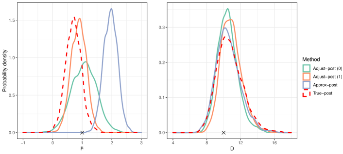
Figure 2: Univariate densities estimates of approximations to the OU Process model posterior distribution for a single dataset. The original approximate posterior (Approx-post) and adjusted posteriors (Adjust-post) with $(\alpha)$ clipping are shown with solid lines. The true posterior (True-post) is shown with a dashed line. The true generating parameter value is indicated with a cross $(\times)$.

For this example we sample from the approximate and true posteriors using the Turing.jl library (Ge et al.,, 2018) in Julia (Bezanson et al.,, 2017). We use the default No-U-Turn Hamiltonian Monte Carlo algorithm (Hoffman et al.,, 2014). For simplicity, we set the stabilizing function $v(\tilde{y})=1$.

The results are presented in Table LABEL:tab:repeated_results_ou. It is clear that the approximate posterior performs poorly for $\mu$. Despite this, the adjustment method is still able to produce results that are similar to the true posterior on average. The approximate method already produces accurate inferences similar to the true posterior for $D$ so that the adjustment is negligible. As an example, the results based on running the adjustment process on a single dataset are shown in Figure 2.

Table 1: Average results for each parameter over 100 independent datasets for the univariate OU process example. The posteriors compared are the original approximate posterior (Approx-post) and adjusted posteriors (Adjust-post) with $(\alpha)$ clipping, and the true posterior (True-post). ¹ 90% target coverage.

	$\mu$				$D$
Method	MSE	Bias	St. Dev.	Cov.1	MSE	Bias	St. Dev.	Cov.1
Approx-post	$1.54$	$1.21$	$0.22$	$0$	$4.73$	$0.18$	$1.46$	$85$
Adjust-post (0)	$0.12$	$0.15$	$0.20$	$64$	$4.83$	$0.28$	$1.24$	$72$
Adjust-post (0.5)	$0.12$	$0.15$	$0.23$	$81$	$5.08$	$0.41$	$1.42$	$81$
Adjust-post (1)	$0.12$	$0.15$	$0.23$	$82$	$5.13$	$0.42$	$1.45$	$83$
True-post	$0.12$	$-0.01$	$0.26$	$94$	$5.00$	$0.37$	$1.48$	$85$

3.1.2 Bivariate OU process with variational approximation

We can define a bivariate OU process by considering $\{Y_{t}\}_{t\geq 0}$ for $Y_{t}\in\mathbb{R}^{2}$, such that the components are $Y_{t,1}=X_{t,1}$ and $Y_{t,2}=\rho X_{t,1}+(1-\rho)X_{t,2}$ where $X_{t,1}$ and $X_{t,2}$ are independent OU processes, conditional on shared parameters $(\mu,\gamma,\sigma)$, and governed by (12). The additional parameter $\rho\in[0,1]$ measures the correlation between $Y_{t,1}$ and $Y_{t,2}$.

Again, we consider the true model for $X_{t,1}$ and $X_{t,2}$ to be defined by (13), therefore $(Y_{t,1},Y_{t,2})$ have joint distribution that is bivariate Gaussian with correlation $\rho$. For the observed data we take 100 independent realizations simulated from the above model with $x_{0,1}=x_{0,2}=5$, $\mu=1$, $\gamma=2$, $T=1$, $\sigma^{2}=20$, and $\rho=0.5$. We assume that $x_{0,1}$, $x_{0,2}$, and $\gamma$ are known and we attempt to infer $\mu$, $D=\sigma^{2}/2$, and $\rho$. We use independent priors where $\mu\sim\text{N}(0,10^{2})$, $D\sim\text{Exp}(1/10)$, and $\rho\sim\text{U}(0,1)$. We use automatic differentiation variational inference (Kucukelbir et al.,, 2017) for the approximate model with a mean-field approximation as the variational family as implemented in Turing.jl. We expect the correction from our method will need to introduce correlation in the posterior due to the independence inherited from the mean-field approximation.

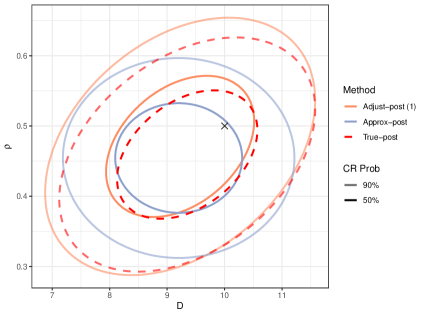
(a) Bivariate density contours of $\rho$ and $D$

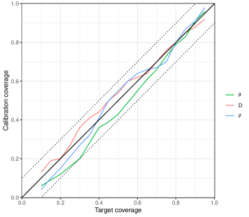
(b) Calibration diagnostic

Figure 3: Summaries of approximations to the bivariate OU Process model posterior distribution for a single dataset. Plot (a) shows 50% and 90% credible region probability (CR Prob) contours from a Gaussian approximation to the bivariate density of $\rho$ and $D$. The original approximate posterior (Approx-post) and adjusted posteriors (Adjust-post) with $(\alpha)$ clipping are shown with solid lines. The true posterior (True-post) is shown with a dashed line. The true generating parameter value is indicated with a cross $(\times)$. Plot (b) shows the calibration checks for all parameters (see Section 2.5) for $\alpha=1$ with $\pm 0.1$ deviation from parity shown with a dotted line.

The variational approximation of the bivariate OU posterior estimates the mean and variance well in this example. The univariate bias, MSE, and coverage metrics are very similar for the approximate, adjusted ($\alpha=1$) and true posteriors (Table LABEL:tab:repeated_results_mv_ou in Appendix E). However the adjusted posterior with $\alpha=0$ is poor due to high variance of the weights, perhaps due to the increased dimension of this example. This could be corrected using an appropriate stabilizing function, but we leave this for future research.

Despite the good univariate properties of the approximate posterior, the choice of a mean-field approximation cannot recover the correlation between the parameters, in particular $\rho$ and $D$. Figure 2(a) shows an example of the independence between $\rho$ and $D$ in the approximate posterior and how the adjusted posterior corrects this (from one dataset). To investigate the methods ability to recover the correlation structure we monitor the empirical correlation between $\rho$ and $D$ over 100 independent trials. The adjusted posterior ($\alpha=1$) was able to produce a mean correlation of 0.37 compared to 0.42 for the true posterior, close to a full recovery. The approximate posterior, on the other hand, has zero correlation because of the mean-field approximation choice. Further correlation summaries are provided in Table LABEL:tab:corr_bi_ou.

We also include Figure 2(b) to demonstrate the calibration diagnostic from Section 2.5 for the same dataset used in Figure 2(a). The calibration coverage is the empirical coverage from the adjusted posteriors on the calibration (simulated) datasets. Here we can see the transformation learned is well calibrated as the calibration coverage is close to the target coverage for the range considered (0.1–0.95).

3.2 Lotka-Volterra Model

We consider the Lotka-Volterra, or predator-prey, dynamics governed by a stochastic differential equation (SDE). In particular, let $\{(X_{t},Y_{t})\}_{t\geq 0}$ be a continuous time stochastic process defined by the SDE

$$\mathrm{d}X_{t}=(\beta_{1}X_{t}-\beta_{2}X_{t}Y_{t})\mathrm{d}t+\sigma_{1}\mathrm{d}B_{t}^{1},\quad\mathrm{d}Y_{t}=(\beta_{4}X_{t}Y_{t}-\beta_{3}Y_{t})\mathrm{d}t+\sigma_{2}\mathrm{d}B_{t}^{2},$$ (14)

where $\{B_{t}^{k}\}_{t\geq 0}$ are independent Brownian noise processes for $k\in\{1,2\}$. For this example, we assume the pairs $(x_{t},y_{t})$ are observed without error at times $t\in\{0,0.1,0.2,\ldots,9.9,10\}$, for a total of $n=101$ observations and fix $\sigma_{1}=\sigma_{2}=0.1$. We use initial values $X_{0}=Y_{0}=1$ and simulate the observations with true parameter values $\beta_{1}=1.5,\beta_{2}=\beta_{4}=1.0,\beta_{3}=3.0$ using the “SOSRI” solver (Rackauckas and Nie,, 2020).

We are motivated by an approximate posterior example appearing in the Turing.jl tutorials (Ge et al.,, 2018; TuringLang,, 2023). It uses an unreferenced method for inference on the parameters of an SDE. Despite its unknown inferential properties, we can correct the approximation using Bayesian Score Calibration and assess the correction using the calibration diagnostics. For the approximate model we use the noisy quasi-likelihood

$$l(\beta_{1:4},\tau~{}|~{}x_{1:n},y_{1:n})=\tau^{2n}\exp\left(-\frac{\tau^{2}}{2}\sum_{i=1}^{n}\left[(x_{i}^{\prime}-x_{i})^{2}+(y_{i}^{\prime}-y_{i})^{2}\right]\right),$$

where $\{(x_{i}^{\prime},y_{i}^{\prime})\}_{i=1}^{n}$ are simulated conditional on the $\beta_{1:4}$ using a rough approximation to the SDE (14). In particular, we use the Euler-Maruyama method with $\Delta t=0.01$. For priors we use $\beta_{i}\overset{\text{iid}}{\sim}\text{U}(0.1,5)$ for $i\in\{1,2,3,4\}$ and ${\tau\sim\text{Gamma}(2,3)}$. The quasi-likelihood is reminiscent of an approximate likelihood used in ABC. In particular, a Gaussian kernel is used to compare observed and simulated data, where $\tau$ plays a similar role to the tolerance in ABC. Usually in ABC, the tolerance is chosen to be small and fixed, but here we take it as random. However, as shown in Bortot et al., (2007), for example, using a random tolerance can enhance mixing of the MCMC chain. The resulting approximate posterior therefore has two levels of approximation; (i) an ABC-like posterior which uses (ii) a coarse approximate simulator rather than the true data generating process (which would require relatively more computation).

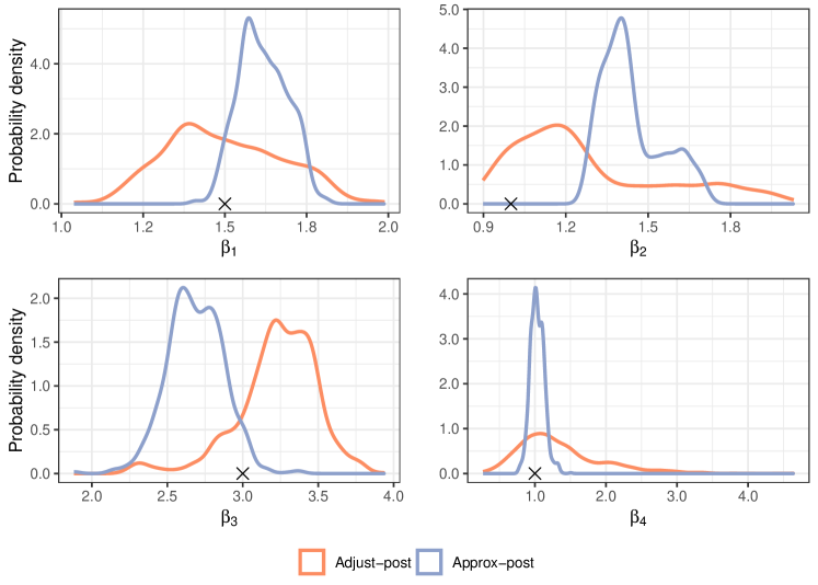
Figure 4: Estimated univariate posterior distributions for the Lotka-Volterra example. Distributions shown are the original approximate posterior (Approx-post) and adjusted posteriors (Adjust-post) with $\alpha=1$ clipping. The true generating parameter value is indicated with a cross $(\times)$.

For the calibration procedure we use $M=200$ calibration datasets and use the unit weight approximation. We draw samples from the approximate posterior using the NUTS Hamiltonian Monte Carlo sampler with 0.25 target acceptance rate since the gradient is noisy. Finally, we use a multivariate moment-correcting transformation with dimension $d=4$ and add a squared penalty term to all parameters of the lower-diagonal scaling matrix $L$. We shrink the diagonal elements of $L$ to one, and off-diagonals elements to zero with rate $\lambda=0.05$.

The results show that the adjusted posterior in this example does significantly better than the approximate posterior. Figure 4 shows the marginal posteriors have much better coverage of the true parameter values and generally increase the variance of the approximate posterior to reflect that the approximation is too precise. Significant bias in parameter $\beta_{2}$ is also corrected. The target 90% coverage estimate from the calibration diagnostic was $(0.32,0.31,0.29,0.37)$ for the approximate posterior, and $(0.68,0.79,0.69,0.97)$ for the adjusted posterior for $(\beta_{1},\beta_{2},\beta_{3},\beta_{4})$ respectively.

Despite overall positive results, the calibration diagnostic shows that caution is required when using this adjusted approximate posterior. Though we see the adjusted posterior has significantly better calibration coverage than the approximate posterior in Figure 5, it still lags the nominal target coverage for parameters $\beta_{1}$ and $\beta_{3}$. Hence a conservative approach should be taken to constructing credible regions for those parameters. The calibration diagnostic is a useful byproduct of our method, alerting users to potential problems.

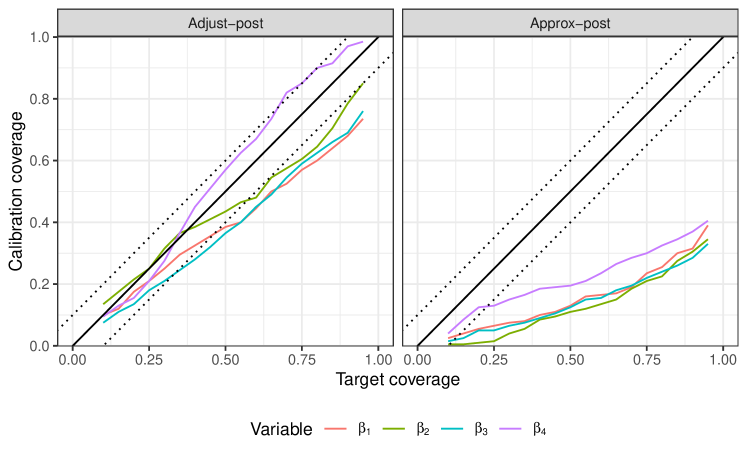
Figure 5: Calibration checks for all parameters in the Lotka-Volterra example for $\alpha=1$ with $\pm 0.1$ deviation from parity shown with a dotted line.

We also note a potential over-correction in the bias of $\beta_{3}$ seen in Figure 4. Investigating this further we find that the calibration samples that were simulated were in the range of $\beta_{3}\in[1.5,2.9]$ which excluded the true parameter value. Hence the transformation learned may have been skewed to this region. Increasing the scale of the importance distribution that generates the calibration samples may help this. Using a more sophisticated transformation or performing the calibration sequentially, as in Pacchiardi and Dutta, (2022), may also be possible in future work. The ranges covered by the importance distribution for the other parameters were $\beta_{1}\in[1.5,2.4],\beta_{2}\in[0.9,2.7]$ and $\beta_{4}\in[0.6,1.1]$. A different importance distribution should be used if one suspects these ranges do not adequately cover the likely values of the true posterior.

4 Discussion

In this paper we have presented a new approach for modifying posterior samples based on an approximate model or likelihood to improve inferences in light of some complex target model. Our approach does not require any likelihood evaluations of the target model, and only a small number of target model simulations and approximate posterior computations, which are easily parallelizable. Our approach is particularly suited to applications where the likelihood of the target model is completely intractable, or if the surrogate likelihood is several orders of magnitude faster to evaluate than the target model.

We focused on correcting inferences from an approximate model, but our approach can also be applied when the inference algorithm is approximate. For example, we could use our approach to adjust inferences from likelihood-free algorithms. We plan to investigate this in more detail in future research.

We propose a straightforward clipping method when we wish to guarantee finite weights in our importance sampling step. However, a more sophisticated approach to clipping is possible, namely Pareto smoothed importance sampling (PSIS, Vehtari et al.,, 2022), which we could use instead of unit weights, if desired. PSIS may be a better approximation to the weights, but would come with additional computational cost.

In general, our method can be used with any proper scoring rule. We concentrated on the energy score because of the ease with which it can be estimated using transformed samples from the approximate distribution. For example, the log-score could also be used by calculating a kernel density estimate from the adjusted posteriors. We found that using $\beta=1$ gives good results in our experiments, but it may be of interest to try the energy score with $\beta\neq 1$ in future work.

In future work we aim to consider more flexible transformations when warranted by deficiencies in the approximate model. This will be particularly important when the direction of the bias in the approximate model changes in different regions of the parameter space. Though learning more flexible transformations will likely necessitate more calibration samples and datasets, and longer optimization time. We note that our method does not require invertible or differentiable transformations, making it quite flexible compared to most transformation-based inference algorithms which require differentiability.

Another limitation of our approach is that we do not necessarily expect our current method to generate useful corrections when the approximate posterior is very poor. A poor approximation would likely lead to a family of kernels that is not sufficiently rich. If the transform is learned in a region of the parameter space far away from the true posterior mass, the calibration datasets are likely to be far away from the observed data, and the transformation may not successfully calibrate the approximate posterior conditional on the observed data. We did provide arguments for when we expect moment-correcting transformations to be asymptotically sufficiently rich and a practical method for detecting insufficiency. However, as already alluded to, a more flexible transform may be able to calibrate more successfully across a wider set of parameter values (e.g. the prior or inflated version of the approximate posterior). We also note that in this paper we assume that the target complex model is correctly specified, and an interesting future direction would consider the case where the target model itself is possibly misspecified.

Appendix A Additional theorems and proofs

A.1 Proof of Theorem 1

Proof.

Denote the objective function in (3) as $E(K)$. Using the Radon-Nikodym derivative $\mathrm{d}\Pi/\mathrm{d}\bar{\Pi}$ we can rewrite this as

$$E(K)=\mathbb{E}_{\theta\sim\Pi}\mathbb{E}_{\tilde{y}\sim P(\cdot~{}|~{}\theta)}\left[v(\tilde{y})S(K(\cdot~{}|~{}\tilde{y}),\theta)\right]=\int\Pi(\mathrm{d}\theta)P(\mathrm{d}\tilde{y}~{}|~{}\theta)v(\tilde{y})S(K(\cdot~{}|~{}\tilde{y}),\theta),$$

then substituting $\Pi(\mathrm{d}\theta)P(\mathrm{d}\tilde{y}~{}|~{}\theta)=P(\mathrm{d}\tilde{y})\Pi(\mathrm{d}\theta~{}|~{}\tilde{y})$ we find that

$$E(K)=Z_{v}\mathbb{E}_{\tilde{y}\sim Q}\mathbb{E}_{\theta\sim\Pi(\cdot~{}|~{}\tilde{y})}\left[S(K(\cdot~{}|~{}\tilde{y}),\theta)\right],$$

where $Q(\mathrm{d}\tilde{y})=P(\mathrm{d}\tilde{y})v(\tilde{y})/Z_{v}$, with $Z_{v}=P(v)\in(0,\infty)$ by assumption.

Now for maximizing $E(K)$, we can ignore the constant $Z_{v}$, and find that

$$K^{\star}=\operatorname*{arg\,max}_{K\in\mathcal{K}}E(K) =\operatorname*{arg\,max}_{K\in\mathcal{K}}\mathbb{E}_{\tilde{y}\sim Q}\mathbb{E}_{\theta\sim\Pi(\cdot~{}|~{}\tilde{y})}\left[S(K(\cdot~{}|~{}\tilde{y}),\theta)\right]$$

$$=\operatorname*{arg\,max}_{K\in\mathcal{K}}\mathbb{E}_{\tilde{y}\sim Q}\left[S(K(\cdot~{}|~{}\tilde{y}),\Pi(\cdot~{}|~{}\tilde{y}))\right].$$

We note that $S(K(\cdot~{}|~{}\tilde{y}),\Pi(\cdot~{}|~{}\tilde{y}))$ is maximized if and only if $K(\cdot~{}|~{}\tilde{y})=\Pi(\cdot~{}|~{}\tilde{y})$ and $K(\cdot~{}|~{}\tilde{y}),\Pi(\cdot~{}|~{}\tilde{y})\in\mathcal{P}$ for fixed $\tilde{y}\in\mathsf{Y}$ since $S$ is a strictly proper scoring rule relative to $\mathcal{P}$. Then under expectation with respect to $Q$, if $\mathcal{K}$ is sufficiently rich, the optima $K^{\star}$ must satisfy $K^{\star}(\cdot~{}|~{}\tilde{y})=\Pi(\cdot~{}|~{}\tilde{y})$ almost surely. ∎

A.2 Proof of Theorem 2

Proof.

Let $g_{z}(x)=\frac{\pi(z)}{\bar{\pi}(z)}\frac{\bar{\pi}(x)}{\pi(x)}$ and consider $v(\tilde{y}_{1:n})=g(\theta^{\ast}_{n})$. Therefore $w(z,\tilde{y}_{1:n})=g_{z}(\theta^{\ast}_{n})$. Applying the continuous mapping theorem with function $h(x)=g_{z}(z)-g_{z}(x)=1-g_{z}(x)$ yields the result. ∎

A.3 A central limit theorem for unit weights

Theorem 3.

Let $g(x)=\bar{\pi}(x)/\pi(x)$ for $x\in\Theta$. If there exists an estimator $\theta^{\ast}_{n}\equiv\theta^{\ast}(\tilde{y}_{1:n})$ such that $\sqrt{n}(\theta^{\ast}_{n}-z)\overset{d}{\rightarrow}\text{N}(0,\Sigma_{z})$ as $n\rightarrow\infty$ when $\tilde{y}_{i}\overset{\text{iid}}{\sim}P(\cdot~{}|~{}z)$ for $z\in\Theta$, $g(\theta^{\ast}_{n})\leq h(\tilde{y}_{1:n})$ a.s. for some integrable function $h$, $g>0$ a.e., and $\nabla g\neq 0$ a.e., then the error from approximating the weights with $\hat{w}=1$ as the size of the data $y_{1:n}$ grows satisfies

$$\sqrt{n}(\hat{w}-w(\theta,\tilde{y}_{1:n}))\overset{d}{\rightarrow}U,$$

$$(U~{}|~{}\theta)\sim\text{N}\left(0,\Sigma_{\theta}^{\prime}\right),\theta\sim\bar{\Pi},$$

as $n\rightarrow\infty$ with choice of stabilizing function $v(\tilde{y}_{1:n})=g(\theta^{\ast}_{n})$, where

$$\Sigma_{\theta}^{\prime}=\nabla\log g(\theta)^{\top}\Sigma_{\theta}\nabla\log g(\theta).$$

Moreover, $\mathbb{E}(U)=0$ and the unit weights $\hat{w}$ therefore have asymptotic distribution with variance equal to $\text{var}(U)=\mathbb{E}_{\theta\sim\bar{\Pi}}(\Sigma_{\theta}^{\prime})$.

Proof.

Take $\theta=z$ fixed and let $g_{z}(x)=\frac{\pi(z)}{\bar{\pi}(z)}\frac{\bar{\pi}(x)}{\pi(x)}$ for $x\in\Theta$. Consider $v(\tilde{y}_{1:n})=g(\theta^{\ast}_{n})$ and therefore $w(z,\tilde{y})=g_{z}(\theta^{\ast}_{n})$. Using the delta method we can deduce that

$$U_{n}(z)\equiv\sqrt{n}(g_{z}(\theta^{\ast}_{n})-g_{z}(z))\overset{d}{\rightarrow}U(z),\qquad\text{where}\;U(z)\sim\text{N}\left(0,\nabla g_{z}(z)^{\top}\Sigma_{z}\nabla g_{z}(z)\right),$$

noting that $g_{z}(\theta^{\ast}_{n})=w(z,\tilde{y})$ and $g_{z}(z)=1=\hat{w}$. Now let $\theta\sim\bar{\Pi}$ on measurable space $(\Theta,\vartheta)$. For all $A\in\vartheta$, consider

$$\lim_{n\rightarrow\infty}\mathsf{P}(U_{n}(\theta)\in A) =\lim_{n\rightarrow\infty}\mathbb{E}_{z\sim\bar{\Pi}}\mathsf{P}(U_{n}(\theta)\in A~{}|~{}\theta=z)$$

$$=\mathbb{E}_{z\sim\bar{\Pi}}\mathsf{P}(U(\theta)\in A~{}|~{}\theta=z)$$

$$=\mathsf{P}(U(\theta)\in A),$$

by the law of total probability and noting that dominated convergence theorem holds since $0<g(\theta^{\ast}_{n})\leq h(y_{1:n})$ implies that $|U_{n}(z)|$ is also dominated. Therefore $U_{n}(\theta)\overset{d}{\rightarrow}U(\theta)$ as $n\rightarrow\infty$ where $U(\theta)\sim\mathbb{E}_{z\sim\bar{\Pi}}U(z)$, i.e. a continuous mixture of Gaussian distributions. Using the continuous mapping theorem we can also state that $U_{n}\overset{d}{\rightarrow}U$ where $U_{n}\equiv-U_{n}(\theta)$ and $U\equiv-U(\theta)$ then noting that $\Sigma_{z}^{\prime}\equiv\nabla g_{z}(z)^{\top}\Sigma_{z}\nabla g_{z}(z)=\nabla\log g(z)^{\top}\Sigma_{z}\nabla\log g(z)$ gives the limiting distribution result. Moreover, we can see $\mathbb{E}(U)=0$ by the law of total expectation and $\text{var}(U)=\mathbb{E}_{z\sim\bar{\Pi}}(\Sigma_{z}^{\prime})$ by the law of total variance. ∎

Remark 3.

If one wishes to estimate the asymptotic variance of the weight approximation, we have freedom to choose the estimator $\theta^{\ast}$. If possible we should choose the estimator that results in the smallest asymptotic variance $\text{var}(U)$ or smallest conditional variance $\Sigma_{\theta}$ if equivalent or more convenient.

Remark 4.

If $\max_{x\in\Theta}g(x)=m<\infty$ then $g(\theta^{\ast}_{n})\leq m$ and the dominating condition holds. This indicates that using a distribution $\bar{\Pi}$ with lighter tails than $\Pi$ is appropriate. Such a statement is surprising as this disagrees with well-established importance sampling guidelines. Moreover, if $\bar{\pi}(\theta)=\hat{\pi}(\theta~{}|~{}y_{1:n})$ then $g(\theta)$ is the approximate likelihood (ignoring the normalizing constant) and a sufficient condition for the domination is that the approximate likelihood $g(\theta)=\hat{p}(y_{1:n}~{}|~{}\theta)$ is bounded. This is the case for any approximate likelihood for which a maximum likelihood estimate exists.

Remark 5.

The dominating condition can also be enforced by only considering bounded $\Theta$. As such the estimator $\theta^{\ast}_{n}$ and hence $g(\theta^{\ast}_{n})$ will typically be bounded. This is the approach taken by Deistler et al., (2022) for sequential neural posterior estimation but no asymptotic justification is given. Our results may be useful in this case, and more generally for this area, but we leave exploration for future research.

Appendix B Further implementation details

B.1 Bayesian score calibration algorithm

The pseudo-code for model calibration is detailed in Algorithm 1, where we use a Monte Carlo approximation of the optimization objective in (6). We assume that the vector of parameters, $\theta$, has support on $\mathbb{R}^{d}$. Should only a subset of parameters in $\theta$ need correcting, Steps 5 and 6 can proceed using only this subset. Steps 5 and 6 can also be performed element-wise if correcting the joint distribution is unnecessary. When $\theta\in S\subset\mathbb{R}^{d}$ we use an invertible transformation to map $\theta$ to $\mathbb{R}^{d}$ in our examples in Section 3. In this case, some care needs to be taken to ensure the weights are calculated correctly in Step 3. After performing the adjustment we can transform back to the original space.

Algorithm 1 Bayesian score calibration using approximate models
Inputs: Number of calibration datasets $M$, number of Monte Carlo samples for estimating scoring rule $N$, importance distribution $\bar{\Pi}$, approximate posterior model $\hat{\Pi}$, scoring rule $S$, transformation function family $\mathcal{F}$, observed dataset $y$. Optional: stabilizing function $v$ (otherwise unit valued) and clipping level $\alpha$ (otherwise no clipping).
Outputs: Estimated optimal transformation function $f^{*}$ and samples from the adjusted approximate posterior based on observed dataset $y$.

1:  Obtain $M$ calibration samples from the importance distribution, $\bar{\theta}^{(m)}\sim\bar{\Pi}(\cdot)$ for $m\in\{1,\ldots,M\}$.

2:  Generate $M$ calibration datasets $\tilde{y}^{(m)}\sim P(\cdot~{}|~{}\bar{\theta}^{(m)})$ for $m\in\{1,\ldots,M\}$.

3:  Calculate weights $\displaystyle w^{(m)}=\frac{\pi(\bar{\theta}^{(m)})}{\bar{\pi}(\bar{\theta}^{(m)})}v(\tilde{y}^{(m)})$ for $m\in\{1,\ldots,M\}$, and clip to $\alpha$ using (9) if specified.If using uniform weights (i.e. $\alpha=1$) then let $w^{(m)}=1$ instead.

4:  Sample from the approximate posterior for each calibration dataset $\hat{\theta}^{(m)}_{i}\sim\hat{\Pi}^{(m)}(\cdot~{}|~{}\tilde{y}^{(m)})$ for $i\in\{1,\ldots,N\}$ and ${m\in\{1,\ldots,M\}}$.

5:  Solve the optimization problem $f^{\star}=\operatorname*{arg\,max}_{f\in\mathcal{F}}\sum_{m=1}^{M}w^{(m)}S^{N}(f_{\sharp}\hat{\Pi}^{(m)},\bar{\theta}^{(m)})$.If using the energy score, use samples from Step 4 to calculate $S^{N}(\cdot,\cdot)$ as per (5).

6:  Generate approximate adjusted samples using push-forward probability measure $f_{\sharp}^{\star}\hat{\Pi}(\cdot~{}|~{}y)$.

B.2 Package and code acknowledgements

A julia package with code that can be applied to any approximate model and data generating process can be found at https://github.com/bonStats/BayesScoreCal.jl, our examples are contained in https://github.com/bonStats/BayesScoreCalExamples.jl.

Our implementation relies heavily on Optim.jl (Mogensen and Riseth,, 2018) and our examples make use of DifferentialEquations.jl (Rackauckas and Nie,, 2017), Distributions.jl (Besançon et al.,, 2021), and Turing.jl (Ge et al.,, 2018).

Appendix C Idealized versus practical weighting functions

An optimal stabilizing function would necessitate that $w(\theta,\tilde{y})=C$, for some constant $C$, though such a function need not exist. However, considering the properties of a theoretical optimal stabilizing function is useful for our asymptotic results in Section 2.4.1. If there were a deterministic function $g$ perfectly predicting $\theta$ from $\tilde{y}$, i.e. $g(\tilde{y})=\theta$ if $\tilde{y}\sim P(\cdot~{}|~{}\theta)$, then $v(\tilde{y})=\bar{\pi}[g(\tilde{y})]/\pi[g(\tilde{y})]$ would be the optimal stabilizing function.

In the absence of such a $g$, we could approximate the stabilizing function by

$$v(\tilde{y})=\frac{\bar{\pi}[\theta^{\star}(\tilde{y})]}{\pi[\theta^{\star}(\tilde{y})]},\quad\theta^{\star}(\tilde{y})=\arg\max_{\vartheta\in\Theta}p(\tilde{y}~{}|~{}\vartheta)\bar{\pi}(\vartheta),$$ (15)

where $\theta^{\star}(\tilde{y})$ is the maximum a posteriori (MAP) estimate of $\theta$ given $\tilde{y}$. The maximum likelihood estimate could also be used. In the case that $\theta^{\star}(\tilde{y})\approx\theta$ we can deduce that $w(\theta,\tilde{y})\approx C$, though deviations from this may be quite detrimental to the variance of the weights. Unfortunately we do not have access to the likelihood $p(\cdot~{}|~{}\cdot)$ so $\theta^{\star}$ is intractable. The approximate likelihood $\hat{p}$ is a practical replacement for $p$ but will be likely to further increase the variance of the weights.

As for the importance distribution, a natural way to concentrate $\theta$ about likely values of the posterior given $y$ is to use $\bar{\Pi}(\cdot)=\hat{\Pi}(\cdot~{}|~{}y)$. This generates datasets $\tilde{y}$ such that they are consistent with $y$ according to the approximate posterior. The idealized setting, with no Monte Carlo error and an accurate MAP using the approximate likelihood, therefore uses

$$v(\tilde{y})=\frac{\bar{\pi}[\theta^{\diamond}(\tilde{y})]}{\pi[\theta^{\diamond}(\tilde{y})]},\quad\theta^{\diamond}(\tilde{y})=\arg\max_{\vartheta\in\Theta}\hat{p}(\tilde{y}~{}|~{}\vartheta)\bar{\pi}(\vartheta),$$ (16)

with $\bar{\Pi}(\cdot)=\hat{\Pi}(\cdot~{}|~{}y)$. If $\theta^{\diamond}(\tilde{y})$ is a biased estimator of $\theta$, we could estimate this bias and correct for it to ensure ${w(\theta,\tilde{y})\approx C}$.

In some cases choosing $\bar{\Pi}(\cdot)=\hat{\Pi}(\cdot~{}|~{}y)$ may be adequate, but it depends crucially on the tail behavior of the ratio $\pi(\theta)/\bar{\pi}(\theta)$ and how well the stabilizing function performs. It may be pertinent to artificially increase the variance of the $\bar{\Pi}$ by transformation or consider an approximation to the chosen distribution with heavier tails.

The simple countermeasure we consider is to truncate or clip the weights (Ionides,, 2008). Truncating the weights is asymptotically consistent if the truncation value $\tau_{M}\rightarrow\infty$ as the number of importance samples $M\rightarrow\infty$. Our examples in Section 3 test clipping the empirical weights, $w^{(m)}$, by

$$w^{(m)}_{\text{clip}}=\min\{w^{(m)},q_{1-\alpha}\},\quad m\in\{1,\ldots,M\},$$ (17)

where the truncation value $q_{1-\alpha}$ is the $100(1-\alpha)$% empirical quantile based on weights $w^{(m)}$. Letting $\alpha\in[0,1]$ depend on $M$ such that $\alpha\rightarrow 0$ as $M\rightarrow\infty$ is sufficient for asymptotic consistency. However, full clipping, i.e. $\alpha=1$ for all $M$, will not satisfy this. Instead, we establish asymptotic consistency (in the size of dataset) for full clipping in Section 2.4.1. In Section 3 we demonstrate good empirical performance with full clipping, effectively removing the importance sampling component and making the approach practically appealing.

Appendix D Additional examples

D.1 Conjugate Gaussian model

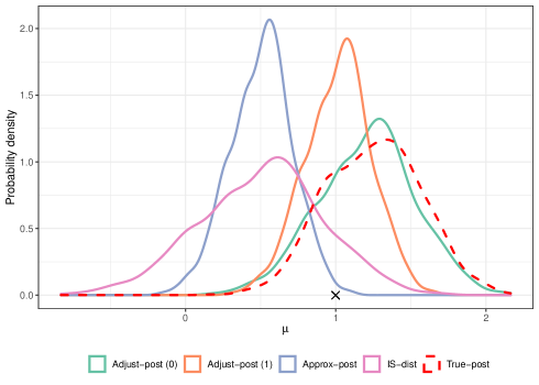
Figure 6: Conjugate Gaussian model univariate densities estimates of approximations to the posterior distribution for a single dataset. The original approximate posterior (Approx-post), importance distribution (IS-dist), and adjusted posteriors (Adjust-post) with $(\alpha)$ clipping are shown with solid lines. The true posterior (True-post) is shown with a dashed line. The true generating parameter value is indicated with a cross $(\times)$.

We first consider a toy conjugate Gaussian example. Here the data $y$ are $n=10$ independent samples from a $\text{N}(\mu,\sigma^{2})$ distribution with $\sigma^{2}=1$ assumed known and $\mu$ unknown. Assuming a Gaussian prior $\mu\sim\text{N}(\mu_{0},\sigma_{0}^{2})$, the posterior is $(\mu|y)\sim\text{N}(\mu_{\mathrm{post}},\sigma_{\mathrm{post}}^{2})$ where

$$\mu_{\mathrm{post}} =\frac{1}{\sigma_{0}^{-2}+n\sigma^{-2}}\left(\frac{\mu_{0}}{\sigma_{0}^{2}}+\frac{\sum_{i=1}^{n}y_{i}}{\sigma^{2}}\right)\mbox{ and }\sigma_{\mathrm{post}}^{2}=\frac{1}{\sigma_{0}^{-2}+n\sigma^{-2}}.$$

We assume this is the target model. For the approximate model, we introduce random error into the posterior mean and standard deviation

$$\mu_{\mathrm{approx}}=\frac{\mu_{\mathrm{post}}-\mu_{\mathrm{error}}}{\sigma_{\mathrm{error}}}\mbox{ and }\sigma_{\mathrm{approx}}=\frac{\sigma_{\mathrm{post}}}{\sigma_{\mathrm{error}}},$$ (18)

where $\mu_{\mathrm{error}}\sim\text{N}(0.5,0.025^{2})$ and $\sigma_{\mathrm{error}}\sim\text{FN}(1.5,0.025^{2})$ and FN denotes the folded-normal distribution. During our simulation the approximate posterior distribution is calculated for each dataset according to (18). The perturbation is random but remains fixed for each dataset. For the stabilizing function we use $v(\tilde{y})=1$ for simplicity.

We coded this simulation in R (R Core Team,, 2021) using exact sampling for the true and approximate posteriors. Results based on 100 independent datasets generated from the model with true value $\mu=1$, and prior parameters $\mu_{0}=0,\sigma_{0}^{2}=4^{2}$ are shown in Table 2. We truncate the weights from the model at quantiles from the empirical weight distribution. We test truncating the weights for $\alpha=0$ (no clipping), $0.25,0.5,0.9$, and $1$ (uniform weights). It can be seen that the adjusted approximation (for all $\alpha$) is a marked improvement over the initial approximation, which is heavily biased and has poor coverage. The estimated posterior distributions based on a single dataset is shown in Figure 6 as an example. We can see that, for this example dataset, the adjusted approximate posteriors are a much better approximation to the true posterior.

Method	MSE	Bias	St. Dev.	Coverage (90%)
Approx-post	$0.48$	$-0.64$	$0.21$	0.24
Adjust-post (0)	$0.21$	$-0.16$	$0.31$	0.99
Adjust-post (0.25)	$0.15$	$-0.18$	$0.26$	0.98
Adjust-post (0.5)	$0.15$	$-0.18$	$0.25$	0.98
Adjust-post (0.9)	$0.14$	$-0.18$	$0.25$	0.98
Adjust-post (1)	$0.14$	$-0.18$	$0.25$	0.98
True-post	$0.16$	$0.02$	$0.31$	1.00

Table 2: Average results over 100 independent observed datasets for the Gaussian example. The posteriors compared are the original approximate posterior (Approx-post), adjusted posteriors (Adjust-post) with $\alpha$ clipping, and the true posterior (True-post).

D.2 Fractional ARIMA model

Let $\{X_{t}\}_{t=1}^{n}$ be a zero-mean equally spaced time series with stationary covariance function $\kappa(\tau,\theta)=\mathbb{E}(X_{t}X_{t-\tau})$ where $\theta$ is a vector of model parameters. Here we consider an autoregressive fractionally integrated moving average model (ARFIMA) model for $\{X_{t}\}_{t=1}^{n}$, described by the polynomial lag operator equation as

$$\phi(L)(1-L)^{d}X_{t}=\vartheta(L)\epsilon_{t},$$

where $\epsilon_{t}\sim\text{N}(0,\sigma^{2})$, $L$ is the lag operator, $\phi(z)=1-\sum_{i=1}^{p}\phi_{i}z_{i}^{i}$ and $\vartheta(z)=1+\sum_{i=1}^{q}\vartheta_{i}z_{i}^{i}$. We denote the observed realized time series as $y=(y_{1},y_{2},\ldots,y_{n})^{\top}$ where $n$ is the number of observations. Here we consider an ARFIMA($p,d,q$) model where $p=2$, $q=1$, and the observed data is simulated with the true parameter $\theta=(\phi_{1},\phi_{2},\vartheta_{1},d)^{\top}=(0.45,0.1,-0.4,0.4)^{\top}$ with $n=15,000$. As in Bon et al., (2021), we impose stationarity conditions by transforming the polynomial coefficients of $\phi(z)$ and $\vartheta(z)$ to partial autocorrelations (Barndorff-Nielsen and Schou,, 1973) taking values on $[-1,1]^{p}$ and $[-1,1]^{q}$ respectively, to which we assign a uniform prior. We apply an inverse hyperbolic tangent transform to map the ARMA parameters to the real line to facilitate posterior sampling. The fractional parameter $d$ has bounds $(-0.5,0.5)$, we sample over the transformed parameter $\tilde{d}=\mbox{tanh}^{-1}(2d)$, and assume that $\tilde{d}\sim\text{N}(0,1)$ a priori.

The likelihood function of the ARFIMA model for large $n$ is computationally intensive. As in, for example, Salomone et al., (2020) and Bon et al., (2021), we use the Whittle likelihood (Whittle,, 1953) as the approximate likelihood to form the approximate posterior. Transforming both the data and the covariance function to the frequency domain enables us to construct the Whittle likelihood with these elements rather than using the time domain as inputs. The Fourier transform of the model’s covariance function, or the spectral density $f_{\theta}(\omega)$, is

$$f_{\theta}(\omega)=\frac{1}{2\pi}\sum_{\tau=-\infty}^{\infty}\kappa(\tau,\theta)\exp(-i\omega\tau),$$

where the angular frequency $\omega\in(-\pi,\pi]$. Whereas the discrete Fourier transform (DFT) of the time series data is defined as

$$J(\omega_{k})=\frac{1}{\sqrt{2\pi}}\sum_{t=1}^{n}X_{t}\exp(-i\omega_{k}t),\quad\omega_{k}=\frac{2\pi k}{n},$$

using the Fourier frequencies $\{\omega_{k}:k=-\lceil n/2\rceil+1,\ldots,\lfloor n/2\rfloor\}$. Using the DFT we can calculate the periodogram, which is an estimate of the spectral density based on the data:

$$\mathcal{I}(\omega_{k})=\frac{|J(\omega_{k})|^{2}}{n}.$$

Then the Whittle log-likelihood (Whittle,, 1953) can be defined as

$$\ell_{\text{whittle}}(\theta)=-\sum_{k=-\lceil n/2\rceil+1}^{\lfloor n/2\rfloor}\left(\log f_{\theta}(\omega_{k})+\frac{\mathcal{I}(\omega_{k})}{f_{\theta}(\omega_{k})}\right).$$

In practice the summation over the Fourier frequencies, $\omega_{k}$, need only be evaluated on around half of the values due to symmetry about $\omega_{0}=0$ and since $f_{\theta}(\omega_{0})=0$ for centred data.

The periodogram can be calculated in $\mathcal{O}(n\log n)$ time, and only needs to be calculated once per dataset. After dispersing this cost, the cost of each subsequent likelihood evaluation is $\mathcal{O}(n)$, compared to the usual likelihood cost for time series (with dense precision matrix) which is $\mathcal{O}(n^{2})$.

Since this example is more computationally intensive, we do not repeat the whole process 100 times in our simulation study. Instead, we fix the observed data and base the repeated dataset results on the 100 calibration datasets (generated from the 100 calibration parameter values) that are produced in a single run of the process. However, we do not validate based on the datasets used in the calibration step, but rather generate 100 fresh datasets from the calibration parameter values. As such, we do not provide a comparison to the true posterior in Table LABEL:tab:repeated_results_whittle as it is fixed and has a high computational cost to sample from. We consider univariate moment-correcting transformations, i.e. $L$ in (8) is diagonal, since the covariance structure is well approximated by the Whittle likelihood in this example. We also choose the stabilizing function to be $v(\tilde{y})=1$ for simplicity.

To generate samples from the approximate and true posterior distributions we use a sequential Monte Carlo sampler (Del Moral et al.,, 2006). In particular, we use likelihood annealing with adaptive temperatures (Jasra et al.,, 2011; Beskos et al.,, 2016) and a Metropolis-Hastings mutation kernel with a multivariate Gaussian proposal. The covariance matrix is learned adaptively as in Chopin, (2002). The simulation is coded in R (R Core Team,, 2021).

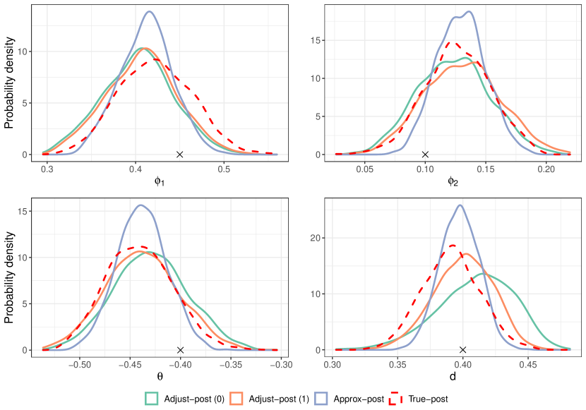
Figure 7: Estimated univariate posterior distributions for the Whittle likelihood example. Distributions shown are the original approximate posterior (Approx-post) and adjusted posteriors (Adjust-post) with $(\alpha)$ clipping. The true posterior (True-post) is shown with a dashed line. The true generating parameter value is indicated with a cross $(\times)$.

The repeated run results for the parameters are shown in Table LABEL:tab:repeated_results_whittle. It is evident that the Whittle approximation performs well in terms of estimating the location of the posterior, but the estimated posterior standard deviation is slightly too small, which leads to some undercoverage. The adjusted posteriors inflate the variance and obtain more accurate coverage of the calibration parameters. An example adjustment for the true dataset is shown in Figure 7, which shows that the adjustment inflates the approximate posterior variance. We also compute the calibration diagnostic, as described in Section 2.5, to confirm the method is performing appropriately on the original data. Figure 8 shows that the calibration coverage is close to the target coverage, across a range of targets, hence the method is performing well.

Table 3: Average results for each parameter over 100 independent calibration datasets (fixed observation dataset) for the Whittle example. The posteriors compared are the original approximate posterior (Approx-post) and adjusted posteriors (Adjust-post) with $(\alpha)$ clipping.

Method	MSE	Bias	St. Dev.	Coverage (90%)
$\phi_{1}$
Approx-post	$0.004$	$0.003$	$0.031$	67
Adjust-post (0)	$0.005$	$-0.007$	$0.041$	83
Adjust-post (0.5)	$0.004$	$-0.003$	$0.041$	83
Adjust-post (1)	$0.005$	$-0.003$	$0.041$	83
$\phi_{2}$
Approx-post	$0.002$	$-0.001$	$0.021$	74
Adjust-post (0)	$0.002$	$-0.007$	$0.031$	86
Adjust-post (0.5)	$0.002$	$0.001$	$0.031$	89
Adjust-post (1)	$0.002$	$0.000$	$0.032$	89
$\vartheta_{1}$
Approx-post	$0.002$	$0.000$	$0.025$	73
Adjust-post (0)	$0.003$	$0.009$	$0.037$	87
Adjust-post (0.5)	$0.003$	$0.000$	$0.036$	88
Adjust-post (1)	$0.003$	$0.000$	$0.037$	88
$d$
Approx-post	$0.001$	$-0.004$	$0.017$	74
Adjust-post (0)	$0.002$	$0.008$	$0.032$	96
Adjust-post (0.5)	$0.001$	$0.000$	$0.024$	89
Adjust-post (1)	$0.001$	$-0.001$	$0.025$	90

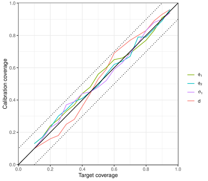
Figure 8: Calibration checks for all parameters in the Whittle likelihood example for $\alpha=1$ with $\pm 0.1$ deviation from parity shown with a dotted line.

Appendix E Additional tables and figures

Table 4: Summary of empirical correlation between parameter samples of $\rho$ and $D$ over 100 independent datasets for the bivariate OU process example. The posteriors compared are the original approximate posterior (Approx-post) and adjusted posteriors (Adjust-post) with $(\alpha)$ clipping, and the true posterior (True-post).

	$\text{corr}(\rho,D)$
Method	Mean	St. Dev.
Approx-post	$0.00$	$0.02$
Adjust-post (0)	$0.18$	$0.41$
Adjust-post (0.5)	$0.37$	$0.16$
Adjust-post (1)	$0.37$	$0.15$
True-post	$0.42$	$0.06$

Table 5: Average results for each parameter over 100 independent datasets for the bivariate OU process example. The posteriors compared are the original approximate posterior (Approx-post) and adjusted posteriors (Adjust-post) with $(\alpha)$ clipping.

Method	MSE	Bias	St. Dev.	Coverage (90%)
$\mu$
Approx-post	$0.10$	$-0.01$	$0.22$	$90$
Adjust-post (0)	$0.12$	$-0.02$	$0.16$	$66$
Adjust-post (0.5)	$0.10$	$-0.01$	$0.22$	$91$
Adjust-post (1)	$0.10$	$-0.01$	$0.22$	$91$
True-post	$0.10$	$-0.01$	$0.22$	$92$
$D$
Approx-post	$2.20$	$0.21$	$1.02$	$84$
Adjust-post (0)	$2.30$	$0.30$	$0.69$	$60$
Adjust-post (0.5)	$2.46$	$0.25$	$1.10$	$85$
Adjust-post (1)	$2.47$	$0.24$	$1.10$	$85$
True-post	$2.54$	$0.27$	$1.16$	$90$
$\rho$
Approx-post	$0.01$	$-0.02$	$0.07$	$86$
Adjust-post (0)	$0.01$	$0.00$	$0.06$	$66$
Adjust-post (0.5)	$0.01$	$0.00$	$0.07$	$90$
Adjust-post (1)	$0.01$	$0.00$	$0.07$	$89$
True-post	$0.01$	$-0.01$	$0.07$	$89$

References

- Barndorff-Nielsen and Schou, (1973) Barndorff-Nielsen, O. and Schou, G. (1973). On the parametrization of autoregressive models by partial autocorrelations. Journal of Multivariate Analysis, 3(4):408–419.
- Beaumont et al., (2002) Beaumont, M. A., Zhang, W., and Balding, D. J. (2002). Approximate Bayesian computation in population genetics. Genetics, 162(4):2025–2035.
- Besançon et al., (2021) Besançon, M., Papamarkou, T., Anthoff, D., Arslan, A., Byrne, S., Lin, D., and Pearson, J. (2021). Distributions.jl: Definition and modeling of probability distributions in the JuliaStats ecosystem. Journal of Statistical Software, 98(16):1–30.
- Beskos et al., (2016) Beskos, A., Jasra, A., Kantas, N., and Thiery, A. (2016). On the convergence of adaptive sequential Monte Carlo methods. The Annals of Applied Probability, 26(2):1111–1146.
- Bezanson et al., (2017) Bezanson, J., Edelman, A., Karpinski, S., and Shah, V. B. (2017). Julia: A fresh approach to numerical computing. SIAM review, 59(1):65–98.
- Bishop, (2006) Bishop, C. M. (2006). Pattern recognition and machine learning, volume 4. Springer, New York, NY.
- Bon et al., (2021) Bon, J. J., Lee, A., and Drovandi, C. (2021). Accelerating sequential Monte Carlo with surrogate likelihoods. Statistics and Computing, 31(5):1–26.
- Bortot et al., (2007) Bortot, P., Coles, S. G., and Sisson, S. A. (2007). Inference for stereological extremes. Journal of the American Statistical Association, 102(477):84–92.
- Brooks et al., (2011) Brooks, S., Gelman, A., Jones, G., and Meng, X.-L. (2011). Handbook of Markov chain Monte Carlo. CRC Press, Boca Raton, FL.
- Chopin, (2002) Chopin, N. (2002). A sequential particle filter method for static models. Biometrika, 89(3):539–552.
- Chopin and Papaspiliopoulos, (2020) Chopin, N. and Papaspiliopoulos, O. (2020). An introduction to sequential Monte Carlo, volume 4. Springer, Cham, Switzerland.
- Cranmer et al., (2020) Cranmer, K., Brehmer, J., and Louppe, G. (2020). The frontier of simulation-based inference. Proceedings of the National Academy of Sciences, 117(48):30055–30062.
- Deistler et al., (2022) Deistler, M., Goncalves, P. J., and Macke, J. H. (2022). Truncated proposals for scalable and hassle-free simulation-based inference. arXiv preprint arXiv:2210.04815.
- Del Moral et al., (2006) Del Moral, P., Doucet, A., and Jasra, A. (2006). Sequential Monte Carlo samplers. Journal of the Royal Statistical Society: Series B (Statistical Methodology), 68(3):411–436.
- Frazier et al., (2022) Frazier, D. T., Nott, D. J., Drovandi, C., and Kohn, R. (2022). Bayesian inference using synthetic likelihood: asymptotics and adjustments. Journal of the American Statistical Association (To appear).
- Ge et al., (2018) Ge, H., Xu, K., and Ghahramani, Z. (2018). Turing: a language for flexible probabilistic inference. In International Conference on Artificial Intelligence and Statistics, AISTATS 2018, 9-11 April 2018, Playa Blanca, Lanzarote, Canary Islands, Spain, pages 1682–1690.
- Gneiting and Raftery, (2007) Gneiting, T. and Raftery, A. E. (2007). Strictly proper scoring rules, prediction, and estimation. Journal of the American Statistical Association, 102(477):359–378.
- Greenberg et al., (2019) Greenberg, D., Nonnenmacher, M., and Macke, J. (2019). Automatic posterior transformation for likelihood-free inference. In Chaudhuri, K. and Salakhutdinov, R., editors, Proceedings of the 36th International Conference on Machine Learning, volume 97 of Proceedings of Machine Learning Research, pages 2404–2414. PMLR.
- Gutmann and Corander, (2016) Gutmann, M. U. and Corander, J. (2016). Bayesian optimization for likelihood-free inference of simulator-based statistical models. Journal of Machine Learning Research, 17:1–47.
- Hoffman et al., (2014) Hoffman, M. D., Gelman, A., et al. (2014). The No-U-Turn sampler: adaptively setting path lengths in Hamiltonian Monte Carlo. Journal of Machince Learning Research, 15(1):1593–1623.
- Ionides, (2008) Ionides, E. L. (2008). Truncated importance sampling. Journal of Computational and Graphical Statistics, 17(2):295–311.
- Jasra et al., (2011) Jasra, A., Stephens, D. A., Doucet, A., and Tsagaris, T. (2011). Inference for Lévy-driven stochastic volatility models via adaptive sequential Monte Carlo. Scandinavian Journal of Statistics, 38(1):1–22.
- Kucukelbir et al., (2017) Kucukelbir, A., Tran, D., Ranganath, R., Gelman, A., and Blei, D. M. (2017). Automatic differentiation variational inference. Journal of Machine Learning Research, 18(14):1–45.
- Lee et al., (2019) Lee, J. E., Nicholls, G. K., and Ryder, R. J. (2019). Calibration procedures for approximate Bayesian credible sets. Bayesian Analysis, 14(4):1245–1269.
- Lei and Bickel, (2011) Lei, J. and Bickel, P. (2011). A moment matching ensemble filter for nonlinear non-Gaussian data assimilation. Monthly Weather Review, 139(12):3964–3973.
- Lueckmann et al., (2017) Lueckmann, J.-M., Gonçalves, P. J., Bassetto, G., Öcal, K., Nonnenmacher, M., and Macke, J. H. (2017). Flexible statistical inference for mechanistic models of neural dynamics. In Proceedings of the 31st International Conference on Neural Information Processing Systems, NIPS’17, page 1289–1299.
- Maruyama, (1955) Maruyama, G. (1955). Continuous Markov processes and stochastic equations. Rendiconti del Circolo Matematico di Palermo, 4:48–90.
- Menéndez et al., (2014) Menéndez, P., Fan, Y., Garthwaite, P. H., and Sisson, S. A. (2014). Simultaneous adjustment of bias and coverage probabilities for confidence intervals. Computational Statistics & Data Analysis, 70:35–44.
- Mogensen and Riseth, (2018) Mogensen, P. K. and Riseth, A. N. (2018). Optim: A mathematical optimization package for Julia. Journal of Open Source Software, 3(24):615.
- Müller, (2013) Müller, U. K. (2013). Risk of Bayesian inference in misspecified models, and the sandwich covariance matrix. Econometrica, 81(5):1805–1849.