Finding Triangles and Other Small Subgraphs
in Geometric Intersection Graphs

Abstract

We consider problems related to finding short cycles, small cliques, small independent sets, and small subgraphs in geometric intersection graphs. We obtain a plethora of new results. For example:

• For the intersection graph of $n$ line segments in the plane, we give algorithms to find a 3-cycle in $O(n^{1.408})$ time, a size-3 independent set in $O(n^{1.652})$ time, a 4-clique in near-$O(n^{24/13})$ time, and a $k$-clique (or any $k$-vertex induced subgraph) in $O(n^{0.565k+O(1)})$ time for any constant $k$; we can also compute the girth in near-$O(n^{3/2})$ time.

• For the intersection graph of $n$ axis-aligned boxes in a constant dimension $d$, we give algorithms to find a 3-cycle in $O(n^{1.408})$ time for any $d$, a 4-clique (or any 4-vertex induced subgraph) in $O(n^{1.715})$ time for any $d$, a size-4 independent set in near-$O(n^{3/2})$ time for any $d$, a size-5 independent set in near-$O(n^{4/3})$ time for $d=2$, and a $k$-clique (or any $k$-vertex induced subgraph) in $O(n^{0.429k+O(1)})$ time for any $d$ and any constant $k$.

• For the intersection graph of $n$ fat objects in any constant dimension $d$, we give an algorithm to find any $k$-vertex (non-induced) subgraph in $O(n\log n)$ time for any constant $k$, generalizing a result by Kaplan, Klost, Mulzer, Roddity, Seiferth, and Sharir (1999) for 3-cycles in 2D disk graphs.

A variety of techniques is used, including geometric range searching, biclique covers, “high-low” tricks, graph degeneracy and separators, and shifted quadtrees. We also prove a near-$\Omega(n^{4/3})$ conditional lower bound for finding a size-4 independent set for boxes.

1 Introduction

In computational geometry, many subquadratic-time algorithms have been developed about finding pairs of geometric objects satisfying some conditions. For example, given $n$ red/blue line segments in 2D, we can find a bichromatic pair of intersecting segments in $O(n^{4/3})$ time [3, 62, 32, 30]. Such results are closely related to geometric range searching [7, 63, 39, 4], and research into subquadratic-time algorithms with fractional exponents for different types of geometric ranges has been explored for decades, and has continued to this day (for just one recent example, see [6]).

But what about problems about finding triples of geometric objects satisfying some pairwise conditions? For example, given $n$ red/blue/green line segments in the plane, how fast can we find a trichromatic triple of line segments such that every two of them intersect? In other words, how fast can we find a trichromatic 3-cycle in the intersection graph? Here, the intersection graph of a set of geometric objects is the undirected graph in which the vertices are the objects and an edge joins two objects iff they intersect. (A 3-cycle is also known as a “triangle” in graph-theoretic terminology, although throughout this paper, except in the title, we will use “3-cycle” or “$C_{3}$”, to avoid confusion with triangles as geometric objects.) We can ask similar questions about quadruples, e.g., finding 4-cycles ($C_{4}$) and 4-cliques ($K_{4}$) in intersection graphs, and $k$-tuples, e.g., finding $k$-cycles ($C_{k}$), $k$-cliques ($K_{k}$), and (induced or not-necessarily-induced) copies of other $k$-vertex subgraphs.

Problems about finding $C_{3}$ and other small subgraphs for general dense or sparse graphs have been extensively studied in the algorithms literature [14, 70, 56, 71, 40, 69, 38] and are well familiar to the SODA audience. In the computational geometry literature, there have been works studying certain standard algorithmic problems on geometric intersection graphs, e.g., connected components [11, 21], all-pairs shortest paths [27, 28], diameter [17], cuts [18], and matchings [16], but surprisingly not as much on the equally fundamental problems of finding $C_{3}$ and other small subgraphs. One can easily envision applications for studying these problems on graphs that are defined geometrically. For example, cycles with a small number of turns in a road network correspond to short cycles in a line-segment intersection graph, and finding a subset in a point set that roughly resembles a fixed pattern may be formulated as finding a small subgraph in some geometric graph. Counting $C_{3}$’s or small cliques provides a popular statistic about graphs in general, and would also be useful for geometric graphs that commonly arise in applications such as unit disk graphs.

Previous work.

The problem of finding $C_{3}$ in geometry-related graphs has been explicitly addressed in at least three previous papers that we are aware of:

• Kaplan et al. [54] in ESA’19 described an $O(n\log n)$-time algorithm for finding a 3-cycle in the intersection graph of $n$ disks in 2D. (They also considered a certain weighted variant of the problem, and related problems such as girth.)

• Agarwal, Overmars, and Sharir [9] in SODA’04 described an $O^{*}(n^{4/3})$-time algorithm for finding a size-3 (or a size-4) independent set in the intersection graph of $n$ unit disks in 2D. This problem is related, since a size-$k$ independent set, which we will denote by “$I_{k}$”, corresponds to a $k$-clique in the complement of the unit disk graph (and of course, a 3-clique is the same as a 3-cycle). Alternatively, in the uncomplemented graph, it can be viewed as an induced copy of the graph consisting of $k$ isolated vertices. (Agarwal et al.’s original motivation was in selecting $k$ “maximally separated” points among $n$ given points.)

• Agarwal and Sharir [10] in SoCG’01 gave an $O^{*}(n^{5/3})$-time algorithm for finding a congruent (i.e., translated and rotated) copy of a fixed triangle $T_{0}$ among $n$ given points in 3D. For example, if $T_{0}$ is the unit equilateral triangle, then this problem is the same as finding a $C_{3}$ in the “unit distance graph”. Note, though, that this particular problem is very sensitive to precision issues, since it is about finding an exact match. (Agarwal and Sharir’s paper for the most part was actually devoted to a combinatorial problem, called the “Erdős–Purdy problem”, of bounding the maximum number of occurrences of a fixed triangle or simplex in a point set.)

In combinatorial geometry, there have been a large body of work (e.g., [47, 48, 64]) about $C_{3}$-free, $K_{k}$-free, or $K_{k,k}$-free geometric intersection graphs or string graphs, for example, bounding the maximum number of edges, or chromatic number, or establishing the existence of good separators. However, the algorithmic question of testing $C_{3}$-freeness or $K_{k,k}$-freeness was not directly addressed in those papers (although some of the techniques there are potentially useful, as we will see).

There have been a few results in computational geometry about finding $k$-cliques for general $k$. For example, Eppstein and Erickson [42] gave an algorithm to find a $K_{k}$ in the intersection graph of $n$ unit disks in 2D in $O(n\log n+k^{2}n\log k)$ time (their motivation was in the related problem of finding $k$ points with minimum diameter among $n$ given points). For any constant $k$ and constant $d$, they also obtained an $O(n\log n)$-time algorithm for finding a $K_{k}$ in the intersection graph of unit balls in $d$D (the hidden dependence on $k$ is exponential). Finding a $K_{k}$ in an intersection graph of $n$ boxes in $d$D reduces to computing the maximum depth, which can be solved in $O(n\log n)$ time for $d=2$ and $\widetilde{O}(n^{d/2})$ time for $d\geq 3$ by techniques for Klee’s measure problem [25]. On the other hand, finding a size-$k$ independent set in an intersection graph of $n$ objects in 2D such as rectangles and line segments takes $n^{O(\sqrt{k})}$ time by using planar-graph separators, or in an intersection graph of $n$ fat objects in $d$D in $n^{O(k^{1-1/d})}$ time by using Smith and Wormald’s geometric separators  [67]. Nearly matching lower bounds [59, 60] of the form $n^{\Omega(k^{1-1/d-\varepsilon})}$ are known even for 2D unit squares or unit disks, assuming the Exponential Time Hypothesis (ETH), implying that such problems are not fixed-parameter tractable with respect to $k$. (There is also an extensive body of work on approximation algorithms for independent set and clique in geometric intersection graphs, which are not directly relevant here and will be ignored.)

Despite all the works noted above, surprisingly there were still no subquadratic algorithms known (to the best of our knowledge) for finding the simplest patterns, like $C_{3}$, in intersection graphs of line segments. This paper will rectify the situation.

New results.

We obtain a plethora of new results, as summarized in Table 1. The 23 new upper bounds are derived from 19 different algorithms or theorems/corollaries! We focus only on the detection versions of these problems: deciding whether a pattern occurs, and if so, reporting one occurrence. We focus on the most basic types of geometric objects, namely, boxes in $d$D, line segments in 2D, and fat objects in $d$D; throughout this paper, the dimension $d$ is always considered a constant. Though not necessarily indicated in the table, some (but not all) of the results hold for more general classes of geometric graphs, and for colored variants of the problems; readers are referred to the theorem statements for the details.

objects	pattern	run time	ref.	notes
boxes in $d$D	$C_{3}$	$O(n^{1.408})$	Thm. 4.6	($\Omega^{*}(n^{4/3})$  Thm. 2.1)
	$I_{3}$	$\widetilde{O}(n)$	Thm. 10.1
	$C_{4}$	$\widetilde{O}(n)$	Thm. 6.1
	$K_{4}$ or any induced $X_{4}$	$O(n^{1.715})$	Thm. 5.6
	$I_{4}$	$\widetilde{O}(n^{3/2})$	Thm. 10.2	($\Omega^{*}(n^{4/3})$  Thm. 2.2)
	$C_{k}$ for $k\equiv 0\bmod 4$	$\widetilde{O}(n^{2-4/k})$	Thm. 6.1
	$C_{k}$ for $k\equiv 2\bmod 4$	$\widetilde{O}(n^{2-4/(k+2)})$	Thm. 6.1
	$C_{k}$ for $k$ odd	$O(n^{2-2/(k+1)})$	Thm. 4.6
	$K_{k}$, $I_{k}$, or any induced $X_{k}$	$O(n^{0.429k+O(1)})$	Cor. 5.7
boxes in 5D	$I_{4}$	$\widetilde{O}(n)$	Thm. 10.3
boxes in 2D	$I_{5}$	$\widetilde{O}(n^{4/3})$	Thm. 10.5
line segments in 2D	$C_{3}$	$O(n^{1.408})$	Thm. 4.7
	$I_{3}$	$O(n^{1.652})$	Thm. 5.3
	trichromatic $C_{3}$	$O^{*}(n^{7/4})$	Thm. 5.1
	$C_{4}$	$\widetilde{O}(n)$	Thm. 6.2
	$K_{4}$	$O^{*}(n^{24/13})$	Thm. 5.9
	$C_{k}$ for $k$ even	$O(n^{1.187})$	Thm. 7.1
	$C_{k}$ for $k$ odd	$O(n^{2-2/(k+1)})$	Thm. 4.7
	girth	$\widetilde{O}(n^{3/2})$	Thm. 7.2
	$K_{k}$ or any induced $X_{k}$	$O(n^{0.565k+O(1)})$	Cor. 5.11
fat objects in $d$D	$C_{k}$, $K_{k}$, or any (non-induced) $X_{k}$	$O(n\log n)$	Thm. 8.3
translates in 2D	$C_{3}$ or $I_{3}$	$\widetilde{O}(n^{3/2})$	Thm. 9.1
translates in 3D	$C_{3}$ or $I_{3}$	$\widetilde{O}(n^{9/5})$	Thm. 9.1

Table 1: Time complexity for finding a small subgraph in a geometric intersection graph. Here, $d$ and $k$ are constants; $C_{k}$ denotes a $k$-cycle; $I_{k}$ denotes a size-$k$ independent set; $K_{k}$ denotes a $k$-clique; and $X_{k}$ denotes an arbitrary fixed $k$-vertex subgraph. “Translates” refer to translated copies of a fixed geometric object of constant description complexity.

As can be seen from the table, we have identified a rich class of problems in computational geometry that are solvable in polynomial time with interesting exponents, going beyond traditional problems about finding pairs of geometric objects. As one can predict, some of these fractional exponents come from the use of geometric range searching, but in far less obvious ways.

A little more surprising, at least at first glance, is that unusual exponents arise even in the case of boxes (e.g., see our results for $K_{4}$ and $I_{4}$), as problems about boxes typically require only orthogonal range searching, which are easier and admit polylogarithmic-time data structures. On the other hand, the aforementioned known results about fixed parameter intractability in terms of $k$, which hold even for 2D unit squares, indicate that time bounds for $I_{k}$ eventually have to be super-linear as the constant $k$ gets sufficiently large (though with Marx et al.’s intractability proofs [59, 60], it seems $k$ needs to be fairly large). We prove that finding $C_{3}$ for 3D boxes or $I_{4}$ for 6D boxes already requires $\Omega^{*}(n^{4/3})$ time, under certain hypotheses from fine-grained complexity. This lower bound for $I_{4}$ in 6D complements nicely with the near-linear upper bounds for $I_{3}$ for any dimension $d$, as well as for $I_{4}$ in 5D.

Some of our algorithms use fast (square or rectangular) matrix multiplication, but some do not. Even for those that use it, weaker but still nontrivial upper bounds can be obtained with naive matrix multiplication. See some of the theorem statements for the time bounds expressed in terms of the matrix multiplication exponent $\omega<2.373$ [12]. There have been several previous examples of the usage of fast matrix multiplication in computational geometry, e.g., on dynamic geometric connectivity [21, 26], shortest paths in geometrically weighted graphs [23], colored orthogonal range counting [55], …, and our work may be viewed as a continuation of this interesting line of research.

Our results on $K_{4}$ for boxes and line segments should be compared with the current best time bound on $K_{4}$ for general graphs, which is $O(n^{\omega(1,2,1)})\leq O(n^{3.252})$ [40]. Our results on $K_{k}$ for boxes and line segments should be compared with the current best bound on $K_{k}$ for general graphs, which is about $O(n^{k\omega/3+O(1)})\leq O(n^{0.791k+O(1)})$ [40]. Our algorithm on $K_{k}$ for boxes is faster than the aforementioned $\widetilde{O}(n^{d/2})$ algorithms if $k$ is small relative to $d$. While $n^{O(\sqrt{k})}$ algorithms were known for $I_{k}$ for 2D boxes and line segments as mentioned, no $n^{o(k)}$ algorithms were known for $I_{k}$, e.g., for arbitrary 3D boxes.

Our $\widetilde{O}(n^{3/2})$ upper bound for computing the girth (i.e., the shortest cycle length) for line-segment intersection graphs contrasts with a recent near-quadratic lower bound on computing the diameter for line-segment intersection graphs by Bringmann et al. [17].

Our $O(n\log n)$ algorithm for finding a (not-necessarily induced) copy of any fixed $k$-vertex subgraph in intersection graphs of fat objects in $d$D, for any constant $k$ and $d$, greatly generalizes the recent result by Kaplan et al. [54], which was only for finding $C_{3}$ in the intersection graph of disks in $\mathbb{R}^{2}$. It is also interesting to compare our result with Eppstein’s well-known result on finding a fixed subgraph in planar graphs in linear time [41] from SODA’95: on one hand, every planar graph can be realized as an intersection graphs of 2D disks by the Koebe–Andreev–Thurston theorem; on the other hand, all of our algorithms require a geometric realization to be given.

Techniques.

For our class of problems, there is actually an abundance of available techniques, and many different ways to combine them. Our contributions lie in collecting all of these techniques together, and in finding the best combination to achieve each of the individual results. We will organize the paper by techniques, which will hopefully help researchers in the future find further improvements and solve more problems of this kind.

One immediate challenge is that intersection graphs may be dense, and so to obtain subquadratic results e.g. for $C_{3}$, we can’t afford to construct the intersection graph explicitly. In Section 4, we describe a known technique, biclique covers (closely related to range-searching data structures), which provides one convenient way to compactly represent intersection graphs. Biclique covers have been used before to directly reduce problems about geometric intersection graphs to problems on non-geometric sparse graphs; for example, see [21] on geometric connectivity. Some readers may have recognized that the $O(n^{1.408})$ bounds in Table 1 for $C_{3}$ are the same as the current known bounds for $C_{3}$ in sparse graphs [14]. Indeed, with biclique covers, we give an easy black-box reduction of $C_{k}$ for boxes (or monochromatic line segments) to $C_{k}$ in sparse graphs. However, the reduction works only for $C_{k}$, but not for $K_{k}$ or other subgraphs. Also, the reduction doesn’t work as well for many types of non-orthogonal objects, such as trichromatic line segments, because the biclique cover complexity is not small enough. Thus, one can’t just blindly apply known results for general sparse graphs to solve geometric problems involving other patterns and other types of objects.

In Section 5, we combine biclique covers and range searching with another technique that may be dubbed “high-low tricks”. Many of the known algorithms for finding small subgraphs in sparse graphs work by dividing into cases based on whether vertices have high degree or low degree. We will do something similar, but instead classifying edges as high or low. We describe a multitude of new algorithms based on this idea. This is the most technically sophisticated part of the paper, as there are multiple possiblilities on how to divide into cases and how to address each case, especially for more complicated patterns such as $K_{4}$.

In Section 6, we exploit the observation that for certain types of geometric objects and certain patterns such as $C_{4}$, the pattern must always occur unless the intersection graph is sparse. But if graph is sparse and, more precisely, has low degeneracy, faster algorithms exist. In Section 7, we further use the fact that for the line segment case in the plane, if the intersection graph is sparse, it must have small separators—this enables efficient divide-and-conquer algorithms. Results in Sections 6 and 7 are less general (for example, they do not apply to colored variants of the problems), although some might actually prefer algorithms that exploit fully the geometry of the specific problems.

In Section 8, we present a different approach for fat objects, by using shifted quadtrees plus dynamic programming. This is more general than Kaplan et al.’s previous approach for disks [54], and conceptually simpler than Eppstein’s for planar graphs [41] as well.

Lastly, in Section 9, we present yet another approach: a round-robin recursion using geometric cuttings, based on one of Agarwal and Sharir’s proofs on the Erdős–Purdy problem [10]. We show that their technique, originally devised for a combinatorial geometry problem, can also be used to obtain new algorithms. However, this technique seems more limited, and currently is responsible only for the results on 2D and 3D translates in Table 1.

We begin with conditional lower bounds in Section 2, as the proofs are short. In particular, the lower bound proof for $I_{4}$ is neat; it is based on the Hyperclique Hypothesis [57], which has started to gain prominence in fine-grained complexity and computational geometry (e.g., see [17]).

2 Conditional Lower Bounds

For certain versions of our problems involving nonorthogonal objects, e.g., trichromatic $C_{3}$ for line segments, it is not difficult to obtain super-linear conditional lower bounds. For example, the well-known Hopcroft’s problem (deciding whether there is a point-line incidence among $n$ points and $n$ lines in 2D) is generally believed to require $\Omega^{*}(n^{4/3})$ time [43, 44], and it is straightforward to reduce Hopcroft’s problem to trichromatic $C_{3}$ for line segments. In this section, we obtain super-linear conditional lower bounds even for versions of the problems for orthogonal objects, namely, boxes, and even for very small $k$.

2.1 $C_{3}$ in 3D box intersection graphs

To warm up, we note an easy reduction from $C_{3}$ in sparse graphs to $C_{3}$ in box intersection graphs. It has been conjectured that finding a $C_{3}$ in a graph with $m$ edges requires $\Omega^{*}(m^{4/3})$ time [2, 1], and so the reduction implies an $\Omega^{*}(n^{4/3})$ lower bound for $C_{3}$ in box intersection graphs under this conjecture. (The running time of the fastest known algorithm [14] is $O(m^{2\omega/(\omega+1)})\leq O(m^{1.408})$ under the current matrix multiplication exponent bound $\omega<2.373$, and is $O^{*}(m^{4/3})$ if $\omega=2$. A stronger “all-edges” variant of the $C_{3}$ finding problem is known to have an $\Omega^{*}(m^{4/3})$ lower bound under more standard conjectures, such as the 3SUM Hypothesis and the APSP Hypothesis [66, 68, 29].) The reduction below is similar to a known conditional lower bound proof for Klee’s measure problem in the 3D case [24].

Theorem 2.1.

If there is an algorithm for finding a $3$-cycle of $n$ boxes in $\mathbb{R}^{3}$ in $T(n)$ time, then there is an algorithm for finding a $3$-cycle in a sparse directed graph with $m$ edges in $O(T(m))$ time.

Proof.

We are given a directed graph $G=(V,E)$ with $m$ edges. Assume the vertices are numbered $\{1,2,\ldots,n\}$. Create the following boxes in $\mathbb{R}^{3}$, for each $(u,v)\in E$: $\{u\}\times\{v\}\times\mathbb{R}$, and $\mathbb{R}\times\{u\}\times\{v\}$, and $\{v\}\times\mathbb{R}\times\{u\}$. (These boxes are technically axis-parallel lines, but can be thickened to be fully 3-dimensional.) It is easy to see that the intersection graph of these $O(m)$ boxes has a 3-cycle iff $G$ has a 3-cycle. ∎

Later in Theorem 4.6, we will prove a reduction in the opposite direction, thus showing equivalence (up to polylogarithmic factors).

2.2 $I_{4}$ in 6D box intersection graphs

For independent set, we prove an $\Omega^{*}(n^{4/3})$ lower bound for size 4, under a different conjecture, that finding a size-$k^{\prime}$ hyperclique in a $k^{\prime\prime}$-uniform hypergraph with $N$ vertices requires $\Omega^{*}(N^{k^{\prime}})$ time, for any constants $k^{\prime}>k^{\prime\prime}\geq 3$. This conjecture is known as the Hyperclique Hypothesis [57] and has been used in a few recent papers (e.g., [17]). In our reduction, we only need the case $k^{\prime}=4$ and $k^{\prime\prime}=3$. Our reduction works for orthants, i.e., $d$-dimensional boxes with $d$ unbounded sides, one per coordinate axis. (Thus, our reduction also works for unit hypercubes, since we can replace orthants with sufficiently large congruent hypercubes, and then rescale).

As we will see, part of the challenge in devising the reduction is in enforcing equalities of certain indices. The disjointness of a pair of orthants basically gives rise to one inequality constraint. Naively one could express each equality as the conjunction of two inequalities, but this is not good enough to make the reduction work for size-4 independent set (where we have only ${4\choose 2}=6$ inequality constraints in total). We initially tried reducing from $C_{4}$ in sparse graphs, unsuccessfully (we can only obtain a lower bound for size-5 independent set this way), but as it turns out, reducing from hypercliques in 3-uniform hypergraphs allows for a more symmetric and elegant proof:

Theorem 2.2.

If there is an algorithm for finding a size-$4$ independent set of $n$ orthants in $\mathbb{R}^{6}$ in $O(n^{4/3-\varepsilon})$ time for some constant $\varepsilon>0$, then there is an algorithm for finding a size-$4$ hyperclique in a $3$-uniform hypergraph with $N$ vertices in $O(N^{4-\varepsilon^{\prime}})$ time for some constant $\varepsilon^{\prime}>0$.

Proof.

By a standard color-coding technique [13], it suffices to consider the 4-hyperclique problem for a 4-partite 3-uniform hypergraph $G=(V,E)$. In other words, $V$ is divided into four sets $X,Y,Z,W$, and we seek four vertices $x\in X$, $y\in Y$, $z\in Z$, and $w\in W$ such that $xyz,yzw,zwx,wxy\in E$.

First, by relabeling, assume that the vertices in $X$ are in $\{1,2,\ldots,N\}$, the vertices in $Y$ are in $\{U,2U,$ $\ldots,NU\}$, the vertices in $Z$ are in $\{U^{2},2U^{2},\ldots,NU^{2}\}$, and the vertices in $W$ are in $\{U^{3},2U^{3},\ldots,NU^{3}\}$, for a sufficiently large integer $U$ (say, $U=N+1$).

Create the following orthants in $\mathbb{R}^{6}$ for each $xy^{\prime}z^{\prime\prime},yz^{\prime}w^{\prime\prime},zw^{\prime}x^{\prime\prime},wx^{\prime}y^{\prime\prime}\in E$, where $x,x^{\prime},x^{\prime\prime}\in X$, $y,y^{\prime},y^{\prime\prime}\in Y$, $z,z^{\prime},z^{\prime\prime}\in Z$, and $w,w^{\prime},w^{\prime\prime}\in W$:

$$\!\!\begin{array}[]{rccccccccccc}\alpha_{xy^{\prime}z^{\prime\prime}}=\!\!\!\!&(-\infty,y^{\prime}\!+\!z^{\prime\prime})&\!\!\!\!\!\times\!\!\!\!\!&\mathbb{R}&\!\!\!\!\!\times\!\!\!\!\!&\mathbb{R}&\!\!\!\!\!\times\!\!\!\!\!&(x\!+\!y^{\prime},\infty)&\!\!\!\!\!\times\!\!\!\!\!&(-\infty,x\!-\!z^{\prime\prime})&\!\!\!\!\!\times\!\!\!\!\!&\mathbb{R}\\ \beta_{yz^{\prime}w^{\prime\prime}}=\!\!\!\!&(y\!+\!z^{\prime},\infty)&\!\!\!\!\!\times\!\!\!\!\!&(-\infty,z^{\prime}\!+\!w^{\prime\prime})&\!\!\!\!\!\times\!\!\!\!\!&\mathbb{R}&\!\!\!\!\!\times\!\!\!\!\!&\mathbb{R}&\!\!\!\!\!\times\!\!\!\!\!&\mathbb{R}&\!\!\!\!\!\times\!\!\!\!\!&(-\infty,y\!-\!w^{\prime\prime})\\ \gamma_{zw^{\prime}x^{\prime\prime}}=\!\!\!\!&\mathbb{R}&\!\!\!\!\!\times\!\!\!\!\!&(z\!+\!w^{\prime},\infty)&\!\!\!\!\!\times\!\!\!\!\!&(-\infty,w^{\prime}\!+\!x^{\prime\prime})&\!\!\!\!\!\times\!\!\!\!\!&\mathbb{R}&\!\!\!\!\!\times\!\!\!\!\!&(x^{\prime\prime}\!-\!z,\infty)&\!\!\!\!\!\times\!\!\!\!\!&\mathbb{R}\\ \delta_{wx^{\prime}y^{\prime\prime}}=\!\!\!\!&\mathbb{R}&\!\!\!\!\!\times\!\!\!\!\!&\mathbb{R}&\!\!\!\!\!\times\!\!\!\!\!&(w\!+\!x^{\prime},\infty)&\!\!\!\!\!\times\!\!\!\!\!&(-\infty,x^{\prime}\!+\!y^{\prime\prime})&\!\!\!\!\!\times\!\!\!\!\!&\mathbb{R}&\!\!\!\!\!\times\!\!\!\!\!&(y^{\prime\prime}\!-\!w,\infty)\end{array}$$

(Open intervals are used here, but they can be avoided easily by slight perturbations of the coordinate values.) We solve the independent set problem on this set $S$ of $O(N^{3})$ orthants.

To see the correctness of this reduction, suppose that $G$ has a 4-hyperclique $\{x,y,z,w\}$ with $x\in X$, $y\in Y$, $z\in Z$, and $w\in W$. Then clearly $\{\alpha_{xyz},\beta_{yzw},\gamma_{zwx},\delta_{wxy}\}$ is a size-4 independent set in $S$.

The other direction is more interesting. Suppose $S$ has a size-4 independent set. Then it must be of the form $\{\alpha_{xy^{\prime}z^{\prime\prime}},\beta_{yz^{\prime}w^{\prime\prime}},\gamma_{zw^{\prime}x^{\prime\prime}},\delta_{wx^{\prime}y^{\prime\prime}}\}$ with $xy^{\prime}z^{\prime\prime},yz^{\prime}w^{\prime\prime},zw^{\prime}x^{\prime\prime},wx^{\prime},y^{\prime\prime}\in E$ and $x\in X$, $y\in Y$, $z\in Z$, and $w\in W$ (since it cannot contain two $\alpha$’s, nor two $\beta$’s, etc.). The pairwise disjointness of these four orthants implies the following 6 constraints:

$$\begin{array}[]{lllllll}y^{\prime}+z^{\prime\prime}&\leq&y+z^{\prime}&&x-z^{\prime\prime}&\leq&x^{\prime\prime}-z\\ z^{\prime}+w^{\prime\prime}&\leq&z+w^{\prime}&&y-w^{\prime\prime}&\leq&y^{\prime\prime}-w\\ w^{\prime}+x^{\prime\prime}&\leq&w+x^{\prime}\\ x^{\prime}+y^{\prime\prime}&\leq&x+y^{\prime}\end{array}$$

Summing the left 4 constraints yields $x^{\prime\prime}+y^{\prime\prime}+w^{\prime\prime}+z^{\prime\prime}\leq x+y+z+w$. On the other hand, summing the right 2 constraints yields $x+y+z+w\leq x^{\prime\prime}+y^{\prime\prime}+w^{\prime\prime}+z^{\prime\prime}$. Thus, we must have equality on all of the constraints. On the other hand, $y^{\prime}+z^{\prime\prime}=y+z^{\prime}$ implies $y^{\prime}=y$ and $z^{\prime\prime}=z^{\prime}$, since $y^{\prime},y\in\{U,2U,\ldots,NU\}$ and $z^{\prime},z^{\prime\prime}\in\{U^{2},2U^{2},\ldots,NU^{2}\}$. Repeating this argument gives us $x=x^{\prime}=x^{\prime\prime}$, $y=y^{\prime}=y^{\prime\prime}$, $z=z^{\prime}=z^{\prime\prime}$, and $w=w^{\prime}=w^{\prime\prime}$. Thus, $xyz,yzw,zwx,wxy\in E$, i.e., $\{x,y,z,w\}$ is a 4-hyperclique in  $G$.

Hence, if the size-4 independent set problem for orthants could be solved in $O(n^{4/3-\varepsilon})$ time, then the 4-hyperclique problem could be solved in $O((N^{3})^{4/3-\varepsilon})=O(N^{4-3\varepsilon})$ time. ∎

3 Preliminaries

From this section onward, we turn to upper bounds, i.e., algorithms. As mentioned, we focus on the detection version of the problems.

Some of our algorithms can solve the colored version of the problems, where the geometric objects are $k$-colored and we seek a $k$-chromatic $k$-vertex pattern. For example, for $C_{k}$, we seek a $k$-cycle that has a vertex of each of the $k$ colors. By a standard color-coding technique [13], the original version reduces to the $k$-colored version while increasing the running time by only an $\widetilde{O}(1)$ factor (assuming that $k$ is a constant). Thus, all results on colored problems are automatically applicable to the original monochromatic problems, but not necessarily vice versa.

Some of our results also hold in a more general setting than intersection graphs. We introduce the following definition:

Definition 3.1.

A $k$-partite range graph is an undirected graph $G=(V,E)$, where $V$ is divided into $k$ parts $V^{(1)},\ldots,V^{(k)}$, and for each $\ell,\ell^{\prime}\in\{1,\ldots,k\}$ with $\ell\neq\ell^{\prime}$, each vertex $u\in V^{(\ell)}$ is associated with a point $p^{(\ell,\ell^{\prime})}(u)$ and each vertex $v\in V^{(\ell^{\prime})}$ is associated with a geometric range $R^{(\ell,\ell^{\prime})}(v)$, such that $uv\in E$ iff $p^{(\ell,\ell^{\prime})}(u)\in R^{(\ell,\ell^{\prime})}(v)$.

Note that since $G$ is undirected, the above definition implicitly requires that $p^{(\ell,\ell^{\prime})}(u)\in R^{(\ell,\ell^{\prime})}(v)$ iff $p^{(\ell^{\prime},\ell)}(v)\in R^{(\ell^{\prime},\ell)}(u)$.

Intersection graphs of boxes can be realized as range graphs, since we can map a box $u=[x_{1},x_{1}^{\prime}]\times\cdots\times[x_{d},x_{d}^{\prime}]\subset\mathbb{R}^{d}$ to a point $p(u)=(x_{1},x_{1}^{\prime},\ldots,x_{d},x_{d}^{\prime})\in\mathbb{R}^{2d}$, and another box $v=[a_{1},a_{1}^{\prime}]\times\cdots\times[a_{d},a_{d}^{\prime}]\subset\mathbb{R}^{d}$ to a range $R(v)=\{(x_{1},x_{1}^{\prime},\ldots,x_{d},x_{d}^{\prime})\in\mathbb{R}^{2d}:\forall i,\ (a_{i}\leq x_{i}\leq a_{i}^{\prime})\ \vee\ (a_{i}\leq x_{i}^{\prime}\leq a_{i}^{\prime})\ \vee\ (x_{i}\leq a_{i}\leq x_{i}^{\prime})\}$. These ranges are all unions of $O(1)$ boxes in $2d$ dimensions. Similarly, intersection graphs of axis-aligned orthogonal polyhedra of $O(1)$ size can be realized as range graphs, where the ranges are unions of $O(1)$ boxes in a larger constant dimension. The complements of these intersection graphs are also range graphs.

Intersection graphs of 2D line segments can also be realized as range graphs, since we can map a line segment $u$ with endpoints $(x,y)$ and $(x^{\prime},y^{\prime})$, slope $\xi$, and intercept $\eta$ to a point $p(u)=(x,y,x^{\prime},y^{\prime},\xi,\eta)\in\mathbb{R}^{6}$, and we can map another line segment $v$ with endpoints $(a,b)$ and $(a^{\prime},b^{\prime})$ to a range $R(v)$ consisting of all points $(x,y,x^{\prime},y^{\prime},\xi,\eta)\in\mathbb{R}^{6}$ such that $(x,y)$ and $(x^{\prime},y^{\prime})$ are on different sides of the line through $(a,b)$ and $(a^{\prime},b^{\prime})$, and $(a,b)$ and $(a^{\prime},b^{\prime})$ are on different sides of the line with slope $\xi$ and intercept $\eta$. These ranges are polyhedral regions of $O(1)$ complexity. Although these regions reside in 6D, they actually have “intrinsic” dimension 2, in the following sense:

Definition 3.2.

Recall that a semialgebraic set $\gamma$ is the set of all points $(x_{1},\ldots,x_{d})\in\mathbb{R}^{d}$ satisfying a Boolean combination of some finite collection of polynomial inequalities in $x_{1},\ldots,x_{d}$. We say that $\gamma$ has intrinsic dimension $d^{\prime}$ if each of these polynomial inequalities depends on at most $d^{\prime}$ of the $d$ variables $x_{1},\ldots,x_{d}$.

Similarly, intersection graphs of 2D triangles or polygons of $O(1)$ size can be realized as range graphs, where the ranges are polyhedral regions of $O(1)$ complexity, dimension $O(1)$, and intrinsic dimension 2. The complements of these intersection graphs are also range graphs.

Note that algorithms for finding $k$-chromatic $K_{k}$ in $k$-partite range graphs can automatically be used to find $k$-chromatic induced or non-induced $X_{k}$ for any $k$-vertex subgraph $X_{k}$ for constant $k$: in $k$-chromatic $K_{k}$, we seek $k$ vertices $v_{1}^{*}\in V^{(1)},\ldots,v_{k}^{*}\in V^{(k)}$ such that $v_{\ell}^{*}v_{\ell^{\prime}}^{*}$ is in the graph for every pair $(\ell,\ell^{\prime})$, but if we want $v_{\ell}^{*}v_{\ell^{\prime}}^{*}$ to be not present in the graph for certain pairs $(\ell,\ell^{\prime})$, we can just take the complement of the bipartite subgraph induced by $V^{(\ell)}\cup V^{(\ell^{\prime})}$, by taking complements of the ranges. (The same cannot be said for algorithms that are specialized to intersection graphs.)

In all our results concerning intersection graphs, we assume that we are given the geometric representation, i.e., the geometric objects. For range graphs, we are given the points $p^{(\ell\ell^{\prime})}(u)$ and ranges $R^{(\ell\ell^{\prime})}(v)$.

4 Technique 1: Biclique Covers

Our first technique involves the notion of biclique covers, which provides a compact representation of graphs and has found many geometric applications (e.g., see [5, 21]):

Definition 4.1.

Given a graph $G=(V,E)$, a biclique cover is a collection of pairs of subsets $\{(A_{1},B_{1}),$ $\ldots,(A_{s},B_{s})\}$, such that $E=\bigcup_{i=1}^{s}(A_{i}\times B_{i})$. The size of the cover refers to $\sum_{i=1}^{s}(|A_{i}|+|B_{i}|)$.

For range graphs where the ranges are orthogonal objects (union of $O(1)$ boxes), it is known that there exist biclique covers of near linear size, by techniques for orthogonal range searching, namely, range trees [7, 39]. (For those familiar with range searching, we think of the right part of the graph as the input point set and the left part as the queries; the $B_{i}$’s are the “canonical subsets” of the data structure, and $A_{i}$ corresponds to the set of all queries whose answers involve the canonical subset $B_{i}$.)

Lemma 4.2.

Consider a bipartite range graph $G=(V,E)$ with $n$ vertices, where where each range is a union of $O(1)$ boxes in a constant dimension. We can compute a biclique cover $\{(A_{1},B_{1}),\ldots,(A_{s},B_{s})\}$ of $\widetilde{O}(n)$ size in $\widetilde{O}(n)$ time. Furthermore, each vertex appears in $\widetilde{O}(1)$ subsets $A_{i}$ and $\widetilde{O}(1)$ subsets $B_{i}$.

For range graphs where the ranges have intrinsic dimension 2, the following lemmas provide two bounds on biclique covers: the first is lopsided (the $A_{i}$’s are sparser than the $B_{i}$’s) and the second is balanced. All but one of our applications will use the first. Both follow from standard techniques on 2D (nonorthogonal) range searching, namely, multi-level cutting trees [36, 7, 63, 4]. For the sake of completeness, we include quick proofs in Appendix A.1–A.2.

Lemma 4.3.

Consider a bipartite range graph $G=(V,E)$ with $n$ vertices, where each range is a semialgebraic set of constant description complexity in a constant dimension, with intrinsic dimension $2$. We can compute a biclique cover $\{(A_{1},B_{1}),\ldots,(A_{s},B_{s})\}$ of $O^{*}(n^{3/2})$ size in $O^{*}(n^{3/2})$ time. Furthermore, each vertex appears in $\widetilde{O}(1)$ subsets $A_{i}$, and for any $r$, the number of subsets $B_{i}$ of size $\Theta(n/r)$ is $O^{*}(r^{2})$.

Lemma 4.4.

Consider a bipartite range graph $G=(V,E)$ with $n$ vertices, where each range is a semialgebraic set of constant description complexity in a constant dimension, with intrinsic dimension $2$. We can compute a biclique cover $\{(A_{1},B_{1}),\ldots,(A_{s},B_{s})\}$ of $O^{*}(n^{4/3})$ size in $O^{*}(n^{4/3})$ time. Furthermore, for any $r$, the number of subsets $A_{i}$ and $B_{i}$ of size $\Theta(n/r)$ is $O^{*}(r^{4/3})$.

Generally, intersection graphs for line segments require biclique cover size $O^{*}(n^{4/3})$. But if the graph is known to be $K_{k}$-free, we observe that near-linear size is possible by adapting known techniques based on segment trees [34]. We include a proof in Appendix A.3.

Lemma 4.5.

Let $k\geq 3$ be a constant. Consider the intersection graph $G$ of $n$ line segments in $\mathbb{R}^{2}$. We can either find a $k$-clique in $G$, or compute a biclique cover $\{(A_{1},B_{1}),\ldots,(A_{s},B_{s})\}$ of $\widetilde{O}(n)$ size, in $\widetilde{O}(n)$ time. Furthermore, in this cover, each element appears in $\widetilde{O}(1)$ subsets $A_{i}$ and $\widetilde{O}(1)$ subsets $B_{i}$.

4.1 $C_{k}$ in box range graphs

As a direct application of biclique covers, we obtain the following result on finding $k$-cycles in box range graphs, and thus, intersection graphs of boxes. Note that the most obvious way to sparsify a graph using biclique covers is to create a new vertex per biclique (as was done, e.g., in [46, 21]), but this would reduce our problem to finding $C_{2k}$ in sparse graphs, which is more expensive than finding $C_{k}$.

Theorem 4.6.

Let $k\geq 3$ be a constant. Consider a $k$-partite range graph $G=(V,E)$ with $n$ vertices, where each range is a union of $O(1)$ boxes in a constant dimension. We can find a $k$-chromatic $k$-cycle in $G$ in $\widetilde{O}(T_{k}(n))$ time, where $T_{k}(m)$ denotes the time complexity for finding a $k$-cycle in a sparse directed graph with $m$ edges.

Proof.

Assume that $V$ is divided into parts $V^{(1)},\ldots,V^{(k)}$. We seek a $k$-cycle $v_{1}^{*}\cdots v_{k}^{*}$ with $v_{1}^{*}\in V^{(1)}$, …, $v_{k}^{*}\in V^{(k)}$ (since all $k!$ cases can be handled similarly).

First, for each $\ell\in[k]$, compute a biclique cover $\{(A_{1}^{(\ell)},B_{1}^{(\ell)}),\ldots,(A_{s}^{(\ell)},B_{s}^{(\ell)})\}$ of $\widetilde{O}(n)$ size for the subgraph of $G$ induced by $V^{(\ell)}\cup V^{(\ell+1)}$, by Lemma 4.2, where $A_{i}^{(\ell)}\subseteq V^{(\ell)}$ and $B_{i}^{(\ell)}\subseteq V^{(\ell+1)}$. (In the superscripts, $k+1$ is considered equivalent to 1.) Define a new directed graph $G^{\prime}$:

• For each $i\in[s]$ and $\ell\in[k]$, create a vertex $z_{i}^{(\ell)}$ in $G^{\prime}$.

• For each $\ell\in[k]$, for each $v\in V^{(\ell+1)}$, for each $B_{i}^{(\ell)}$ containing $v$ and each $A_{j}^{(\ell+1)}$ containing $v$, create an edge from $z_{i}^{(\ell)}$ to $z_{j}^{(\ell+1)}$ in $G^{\prime}$.

The problem then reduces to finding a $k$-cycle in $G^{\prime}$. Since each vertex appears in $\widetilde{O}(1)$ subsets $A_{i}^{(\ell+1)}$, the graph $G^{\prime}$ has $\widetilde{O}(n)$ edges and can be constructed in $\widetilde{O}(n)$ time. ∎

According to known results on finding short cycles in sparse directed graphs:

• $T_{3}(m)=O(m^{2\omega/(\omega+1)})\leq O(m^{1.408})$ by Alon, Yuster, and Zwick [14];

• $T_{4}(m)=O(m^{(4\omega-1)/(2\omega+1)})\leq O(m^{1.478})$ and $T_{5}(m)=O(m^{3\omega/(\omega+2)})\leq O(m^{1.628})$ by Yuster and Zwick [71];

• $T_{k}(m)=O(m^{2-2/k})$ if $k$ is even, and $T_{k}(m)=O(m^{2-2/(k+1)})$ if $k$ is odd, by Alon, Yuster, and Zwick [14] (see Dalirrooyfard, Vuong, and Vassilevska W. [38] for further small improvements depending on $\omega$).

4.2 $C_{k}$ in 2D segment intersection graphs

A similar result can be obtained for intersection graphs of line segments:

Theorem 4.7.

Let $k\geq 3$ be a constant. Given $n$ line segments in $\mathbb{R}^{2}$, we can find a $k$-cycle in the intersection graph in $\widetilde{O}(T_{k}(n))$ time, where $T_{k}(m)$ denotes the time complexity for finding a $k$-cycle in a sparse directed graph with $m$ edges.

Proof.

By color coding [13], it suffices to solve a colored version of the problem, where the input line segments have been colored with $k$ colors, and we seek a $k$-cycle, under the assumption that there exists a $k$-chromatic $k$-cycle. (The $k$-cycle found need not be $k$-chromatic.)

We follow the same approach as in the proof of Theorem 6.1. The only change is that we use Lemma 4.5 for the biclique cover computation. If the lemma fails to compute a cover but instead finds a $K_{k}$, then we have found a $k$-cycle. ∎

Unfortunately, this approach does not directly yield subquadratic algorithms for trichromatic $C_{3}$ or $I_{3}$ for line segments or other types of objects; for example, for $C_{3}$ for line segments, we could apply the $O^{*}(n^{3/2})$-size biclique cover from Lemma 4.3 (as we need the property that each vertex appears in $\widetilde{O}(1)$ of the $A_{i}$’s), but the resulting time bound would be near $(n^{3/2})^{1.408}$, which is superquadratic!

5 Technique 2: High-Low Tricks

In this section, we describe algorithms based on combining biclique covers with the following kind of tricks: dividing into cases based on whether edges in the solution are “high” or “low”, and at the end, choosing parameters to balance cost of the different cases. There are many options in how to divide into cases and how to handle these cases efficiently, making it a challenge to find the best time bounds (we have actually discarded many slower alternatives before arriving at the final algorithms presented here).

One interesting additional idea, used in some of our algorithms for the low cases, is to treat a pair or tuple of objects as one “compound” object. From these compound objects, we can then apply range searching results or invoke earlier algorithms to find a smaller pattern involving fewer objects. Here, generalizations to range graphs become crucial, even if we originally only care about intersection graphs.

5.1 $C_{3}$ in 2D range graphs

As a first example of the “high-low” approach, we describe an $O^{*}(n^{7/4})$-time algorithm for finding $C_{3}$ in range graphs with intrinsic dimension 2. As mentioned, achieving subquadratic time is more challenging here because the biclique cover size is larger. To address the low case, we will use the idea of treating a pair as an object. Below, we will state our result in a more general unbalanced setting because it will be needed in a later algorithm, but the reader may choose to focus on the main case when $n^{\prime}=n$.

Theorem 5.1.

Consider a tripartite range graph $G=(V,E)$ where the first two parts have $O(n)$ vertices and the third part has $O(n^{\prime})$ vertices, and each range is a semialgebraic set of constant description complexity in a constant dimension, with intrinsic dimension $2$. We can find a $3$-cycle in $G$ in $O^{*}(n(n^{\prime})^{3/4})$ time, assuming that $n^{4/5}\leq n^{\prime}\leq n^{4}$.

Proof.

Assume that $V$ is divided into parts $V^{(1)},V^{(2)},V^{(3)}$. We seek a 3-cycle $C^{*}=v_{1}^{*}v_{2}^{*}v_{3}^{*}$ with $v_{1}^{*}\in V^{(1)},\ldots,v_{3}^{*}\in V^{(3)}$.

First, compute a biclique cover $\{(A_{1},B_{1}),\ldots,(A_{s},B_{s})\}$ of $O^{*}(n^{4/3})$ size for the subgraph of $G$ induced by $V^{(1)}\cup V^{(2)}$, by Lemma 4.4, where $A_{i}\subseteq V^{(1)}$ and $B_{i}\subseteq V^{(2)}$.

Let $r\leq n$ be a parameter. Call an edge $uv\in E$ low if $u\in A_{i}$ and $v\in B_{i}$ for some $i$ with $\mu_{i}:=|A_{i}|+|B_{i}|\leq n/r$, and high otherwise. Since the number of $i$’s with $\mu_{i}=\Theta(n/(2^{j}r))$ is $O^{*}((2^{j}r)^{4/3})$, the number of low edges is $O^{*}(\sum_{j\geq 0}(2^{j}r)^{4/3}(n/(2^{j}r))^{2})=O^{*}(n^{2}/r^{2/3})$. We consider two cases:

• Case 1: $v_{1}^{*}v_{2}^{*}$ is low. For each low edge $v_{1}v_{2}$, it suffices to test whether there exists $v_{3}\in V^{(3)}$ such that $v_{1}v_{3}\in E$ and $v_{2}v_{3}\in E$, i.e., the point $(p^{(3,1)}(v_{3}),p^{(3,2)}(v_{3}))$ is in the range $R^{(3,1)}(v_{1})\times R^{(3,2)}(v_{2})$. These tests reduce to $Q=O^{*}(n^{2}/r^{2/3})$ range searching queries on $O(n^{\prime})$ points in a constant dimension, with intrinsic dimension 2. By known range searching results [61, 62, 8, 7, 63, 4], these queries can be answered in time $O^{*}((n^{\prime}Q)^{2/3}+n^{\prime}+Q)=O^{*}(n^{4/3}(n^{\prime})^{2/3}/r^{4/9}+n^{\prime}+n^{2}/r^{2/3})$.

• Case 2: $v_{1}^{*}v_{2}^{*}$ is high. Guess the index $i$ with $\mu_{i}>n/r$, such that $(v_{1}^{*},v_{2}^{*})\in A_{i}\times B_{i}$. There are $O^{*}(r^{4/3})$ choices for $i$. For each $v_{3}\in V^{(3)}$, we test whether there exists $v_{1}\in A_{i}$ such that $v_{1}v_{3}\in E$, i.e., $v_{1}$ is in the range $R^{(3,1)}(v_{3})$, and similarly test whether there exists $v_{2}\in B_{i}$ such that $v_{2}v_{3}\in E$, i.e., $v_{2}$ is in the range $R^{(3,2)}(v_{3})$. If both tests return true, we have found a 3-cycle $v_{1}v_{2}v_{3}$ (since there is an edge between any $v_{1}\in A_{i}$ and any $v_{2}\in B_{i}$). These tests reduce to $O(n^{\prime})$ range searching queries on $O(\mu_{i})$ points, with intrinsic dimension 2. By known range searching results, these queries can be answered in $O^{*}((n^{\prime}\mu_{i})^{2/3}+n^{\prime}+\mu_{i})$ time. Recall that the number of $i$’s with $\mu_{i}=\Theta(2^{j}n/r)$ is $O^{*}((r/2^{j})^{4/3})$. Summing over all $i$, we get the total time bound $O^{*}(\sum_{j\geq 0}(r/2^{j})^{4/3}\cdot((n^{\prime}(2^{j}n/r))^{2/3}+n^{\prime}+2^{j}n/r))=O^{*}(n^{2/3}(n^{\prime})^{2/3}r^{2/3}+n^{\prime}r^{4/3}+nr^{1/3})$.

We set $r=n^{3/4}/(n^{\prime})^{3/16}$ to equalize $n^{\prime}r^{4/3}$ with $n^{4/3}(n^{\prime})^{2/3}/r^{4/9}$. The terms $n^{2/3}(n^{\prime})^{2/3}r^{2/3}$ and $n^{2}/r^{2/3}$ do not dominate if $n^{\prime}\geq n^{4/5}$. ∎

5.2 $I_{3}$ in 2D segment intersection graphs

The preceding algorithm can immediately be used to find size-3 independent sets for line-segment intersection graphs, because the complement graph can be realized as a range graph with intrinsic dimension 2. But in this subsection, we will present a different high-low division that yields a faster algorithm. It is interesting that already for $k=3$, there are very different ways to apply the high-low trick.

We first note in the following lemma that size-2 independent sets are easy to find for line segments:

Lemma 5.2.

Given $n$ red/blue line segments in $\mathbb{R}^{2}$, we can find a bichromatic pair of nonintersecting line segments in $\widetilde{O}(n)$ time.

Proof.

We seek a red segment $s_{1}^{*}$ and a blue segment $s_{2}^{*}$ that do not intersect. There are 4 possibilities: (i) $s_{1}^{*}$ is above the line through $s_{2}^{*}$, (ii) $s_{1}^{*}$ is below the line through $s_{2}^{*}$, (iii) $s_{2}^{*}$ is above the line through $s_{1}^{*}$, or (iv) $s_{2}^{*}$ is above the line through $s_{1}^{*}$. It suffices to consider case (iv), since the other cases can be handled similarly.

Let $p_{1}^{*}$ and $q_{1}^{*}$ be the left and right endpoints of $s_{1}^{*}$. Case (i) can be further broken into two subcases: (a) $p_{1}^{*}$ is above the line through $s_{2}^{*}$ and the slope of $s_{1}^{*}$ is greater than the slope of $s_{2}^{*}$, or (b) $q_{1}^{*}$ is above the line through $s_{2}^{*}$ and the slope of $s_{1}^{*}$ is less than the slope of $s_{2}^{*}$. It suffices to consider case (a).

To this end, we maintain the upper hull ${\cal H}_{\mu}$ of the set of the left endpoints $p_{1}$ of all red segments $s_{1}$ with slope greater than $\mu$, as $\mu$ decreases from $\infty$ to $-\infty$. The hull undergoes $O(n)$ insertions of points, and can be maintained in $O(\log n)$ time per insertion by a known incremental convex hull algorithm [65]. For each blue segment $s_{2}$ with slope $m$, we just check whether there exists a vertex $p_{1}$ of ${\cal H}_{m}$ that is above the line through $s_{2}$, in $O(\log n)$ time by binary search. The total running time is $O(n\log n)$. ∎

Theorem 5.3.

Given $n$ red/blue/green line segments in $\mathbb{R}^{2}$, we can find a trichromatic size-$3$ independent set in $\widetilde{O}(n^{4\omega/(2\omega+1)})\leq O(n^{1.652})$ time.

Proof.

Let $G=(V,E)$ denote the complement of the intersection graph. Let $V^{(1)},V^{(2)},V^{(3)}$ be the color classes. We seek a 3-cycle $C^{*}=v_{1}^{*}v_{2}^{*}v_{3}^{*}$ in $G$ with $v_{1}^{*}\in V^{(1)}$, …, $v_{3}^{*}\in V^{(3)}$.

First, for each $\ell\in[3]$, compute a biclique cover $\{(A_{1}^{(\ell)},B_{1}^{(\ell)}),\ldots,(A_{s}^{(\ell)},B_{s}^{(\ell)})\}$ of $O^{*}(n^{3/2})$ size for the subgraph of $G$ induced by $V^{(\ell)}\cup V^{(\ell+1)}$, by Lemma 4.3. (The “lopsided” form of biclique cover turns out to be better here. In the superscripts, 4 is considered equivalent to 1.)

Let $r\leq n$ be a parameter. Call an edge $uv\in E$ low if $u\in A_{i}^{(\ell)}$ and $v\in B_{i}^{(\ell)}$ for some $i$ with $|B_{i}^{(\ell)}|\leq n/r$, and high otherwise. The number of low edges is $\widetilde{O}(n^{2}/r)$, since each vertex appears in $\widetilde{O}(1)$ subsets $A_{i}^{(\ell)}$. We consider two cases:

• Case 1: At least one edge of $C^{*}$ is low. Say it is $v_{1}^{*}v_{2}^{*}$. First, for each $i$, compute the subset $X_{i}=\{v_{1}\in V^{(1)}:\mbox{$v_{1}v_{2}$ is a low edge and $v_{2}\in A_{i}^{(2)}$}\}$. Since each vertex appears in $\widetilde{O}(1)$ subsets $A_{i}^{(2)}$, we have $\sum_{i}|X_{i}|=\widetilde{O}(n^{2}/r)$ and the $X_{i}$’s can be generated in $\widetilde{O}(n^{2}/r)$ time.

  Guess the index $i$ such that $(v_{2}^{*},v_{3}^{*})\in A_{i}^{(2)}\times B_{i}^{(2)}$. We check whether there exists an edge between $X_{i}$ and $B_{i}^{(2)}$. By Lemma 5.2, this takes $\widetilde{O}(|X_{i}|+|B_{i}^{(2)}|)$ time. If such an edge is found between $v_{1}\in X_{i}$ and $v_{3}\in B_{i}^{(2)}$, then since $v_{1}$ is adjacent to some $v_{2}\in A_{i}^{(2)}$, we have found a 3-cycle $v_{1}v_{2}v_{3}$. Summing over all $i$, we get the total time bound $O^{*}(n^{2}/r+n^{3/2})$.

• Case 2: All three edges of $C^{*}$ are high. We follow the approach in the proof of Theorem 4.6. Define a new directed graph $G^{\prime}$:

  • For each $i\in[s]$ and $\ell\in[3]$ with $|B_{i}^{(\ell)}|>n/r$, create a vertex $z_{i}^{(\ell)}$ in $G^{\prime}$.

  • For each $v\in V$ and $\ell\in[3]$, for each $B_{i}^{(\ell)}$ containing $v$ and each $A_{j}^{(\ell+1)}$ containing $v$, if $z_{i}^{(\ell)}$ and $z_{j}^{(\ell+1)}$ exist, create an edge from $z_{i}^{(\ell)}$ to $z_{j}^{(\ell+1)}$ in $G^{\prime}$.

  The problem then reduces to finding a 3-cycle in $G^{\prime}$. Since each vertex appears in $\widetilde{O}(1)$ subsets $A_{j}^{(\ell+1)}$, the graph $G^{\prime}$ can be constructed in time $\widetilde{O}(\sum_{i,\ell:\,|B_{i}^{(\ell)}|>n/r}|B_{i}^{(\ell)}|)=O^{*}(\sum_{j\geq 0}(r/2^{j})^{2}\cdot(2^{j}n/r))=O^{*}(nr)$ (recalling that the number of $i$’s with $|B_{i}^{(\ell)}|=\Theta(2^{j}n/r)$ is $O((r/2^{j})^{2})$). Since $G^{\prime}$ has $\widetilde{O}(r^{2})$ vertices, we can detect a 3-cycle in $G^{\prime}$ by matrix multiplication in $\widetilde{O}((r^{2})^{\omega})$ time.

We set $r=n^{2/(2\omega+1)}$ to equalize $r^{2\omega}$ with $n^{2}/r$. ∎

5.3 $K_{4}$ (and $K_{k}$) in box range graphs

We now present a subquadratic algorithm for finding 4-cliques for boxes. The details will now get more elaborate. The key idea in the low case is to treat a pair as an object so as to reduce to a $C_{3}$ problem. The high case has many options; the best way we have come up with is to guess away two edges of $K_{4}$ so as to reduce to $C_{4}$ subproblems.

First, as subroutines, we need variants of the known $\widetilde{O}(m^{1.408})$-time algorithm for $C_{3}$ and a known $\widetilde{O}(m^{3/2})$-time algorithm for $C_{4}$ in a sparse graph by Alon, Yuster, and Zwick [14], when the graph is 3- or 4-partite and is lopsided, as stated in the two lemmas below. The generalizations are straightforward and are shown in Appendix A.4–A.5. (Note that when $m=m^{\prime}$, the expression $\min_{\Delta}(m\Delta+M(m/\Delta,m/\Delta,m/\Delta))$ indeed recovers the $O(m^{1.408})$ bound under the current matrix multiplication exponent.)

Lemma 5.4.

Consider a tripartite graph $G$, where the vertices are divided into parts $V^{(1)},V^{(2)},V^{(3)}$, and there are $O(m)$ edges between $V^{(1)}$ and $V^{(2)}$, $O(m)$ edges between $V^{(2)}$ and $V^{(3)}$, and $O(m^{\prime})$ edges between $V^{(3)}$ and $V^{(1)}$. Then we can find a $3$-cycle in $G$ in $O(m^{\prime}\Delta+M(m/\Delta,m^{2}/(\Delta m^{\prime}),m/\Delta))$ time for any given $\Delta$, where $M(n_{1},n_{2},n_{3})$ is the complexity of multiplying an $n_{1}\times n_{2}$ with an $n_{2}\times n_{3}$ matrix.

Lemma 5.5.

Consider a $4$-partite graph $G$, where the vertices are divided into parts $V^{(1)},V^{(2)},V^{(3)},V^{(4)}$, and there are $O(m)$ edges between $V^{(1)}$ and $V^{(2)}$, $O(m^{\prime})$ edges between $V^{(2)}$ and $V^{(3)}$, $O(m)$ edges between $V^{(3)}$ and $V^{(4)}$, and $O(m^{\prime})$ edges between $V^{(4)}$ and $V^{(1)}$. Then we can find a $4$-chromatic $4$-cycle in $G$ in $O(m\sqrt{m^{\prime}}+m^{\prime}\sqrt{m})$ time.

Theorem 5.6.

Consider a $4$-partite range graph $G=(V,E)$ with $n$ vertices, where each range is a union of $O(1)$ boxes in a constant dimension. We can find a $4$-clique in $G$ in $O(n^{1.715})$ time (or in $\widetilde{O}(n^{12/7})$ time if $\omega=2$).

Proof.

Assume that $V$ is divided into parts $V^{(1)},\ldots,V^{(4)}$. We seek a 4-clique $K^{*}=\{v_{1}^{*},\ldots,v_{4}^{*}\}$ with $v_{1}^{*}\in V^{(1)}$, …, $v_{4}^{*}\in V^{(4)}$.

First, for each $\ell,\ell^{\prime}\in[4]$ with $\ell\neq\ell^{\prime}$, compute a biclique cover $\{(A_{1}^{(\ell,\ell^{\prime})},B_{1}^{(\ell,\ell^{\prime})}),\ldots,(A_{s}^{(\ell,\ell^{\prime})},B_{s}^{(\ell,\ell^{\prime})})\}$ of $\widetilde{O}(n)$ size for the subgraph of $G$ induced by $V^{(\ell)}\cup V^{(\ell^{\prime})}$, by Lemma 4.2, where $A_{i}^{(\ell,\ell^{\prime})}\subseteq V^{(\ell)}$ and $B_{i}^{(\ell,\ell^{\prime})}\subseteq V^{(\ell^{\prime})}$.

Let $r\leq n$ be a parameter. Call an edge $uv\in E$ low if $u\in A_{i}^{(\ell,\ell^{\prime})}$ and $v\in B_{i}^{(\ell,\ell^{\prime})}$ for some $i$ with $\mu_{i}^{(\ell,\ell^{\prime})}:=|A_{i}^{(\ell,\ell^{\prime})}|+|B_{i}^{(\ell,\ell^{\prime})}|\leq n/r$, and high otherwise. The number of low edges is $\widetilde{O}(n^{2}/r)$. We consider two cases:

• Case 1: At least one edge of $K^{*}$ is low. Say it is $v_{1}^{*}v_{2}^{*}$. Define a tripartite graph $\widehat{G}$:

  • Each low edge $v_{1}v_{2}$ with $v_{1}\in V^{(1)}$ and $v_{2}\in V^{(2)}$ is a vertex in $G^{\prime}$. Each vertex in $V^{(3)}$ is a vertex in $\widehat{G}$. Each vertex in $V^{(4)}$ is a vertex in $\widehat{G}$.

  • Create an edge between $v_{1}v_{2}$ and $v_{3}\in V^{(3)}$ in $\widehat{G}$ iff $v_{1}v_{3}\in E$ and $v_{2}v_{3}\in E$. Create an edge between $v_{1}v_{2}$ and $v_{4}\in V^{(4)}$ in $\widehat{G}$ iff $v_{1}v_{4}\in E$ and $v_{2}v_{4}\in E$. Create an edge between $v_{3}\in V^{(3)}$ and $v_{4}\in V^{(4)}$ in $\widehat{G}$ iff $v_{3}v_{4}\in E$.

  The problem then reduces to finding a 3-cycle in $\widehat{G}$. Note that $\widehat{G}$ can be realized as a range graph, since the condition “$v_{1}v_{3}\in E$ and $v_{2}v_{3}\in E$” is true iff the point $(p^{(1,3)}(v_{1}),p^{(2,3)}(v_{2}))$ lies in the range $R^{(1,3)}(v_{3})\times R^{(2,3)}(v_{3})$, iff the point $(p^{(3,1)}(v_{3}),p^{(3,2)}(v_{3}))$ lies in the range $R^{(3,1)}(v_{1})\times R^{(3,2)}(v_{2})$. The condition “$v_{1}v_{4}\in E$ and $v_{2}v_{4}\in E$” is similar. These ranges are all unions of $O(1)$ boxes in some constant dimension. We can thus follow the approach in the proof of Theorem 4.6 to reduce 3-cycle detection in $\widehat{G}$ to 3-cycle detection in some new graph $G^{\prime}$. Now, $\widehat{G}$ is a tripartite graph, where the first part has $\widetilde{O}(n^{2}/r)$ vertices and the second and third parts have $O(n)$ vertices. In this unbalanced scenario, the graph $G^{\prime}$ constructed in the proof of Theorem 4.6 is tripartite, where there are $m=O(n)$ edges between the first and the second part and between the second and third part, and $m^{\prime}=\widetilde{O}(n^{2}/r)$ edges between the third and first part. By Lemma 5.4, we can solve the problem in $O(n^{2}\Delta/r+M(n/\Delta,r/\Delta,n/\Delta))$ time.

• Case 2: All edges of $K^{*}$ are high. In particular, $v_{1}^{*}v_{3}^{*}$ and $v_{2}^{*}v_{4}^{*}$ are high. Guess the index $i$ with $\mu_{i}^{(1,3)}>n/r$, such that $(v_{1}^{*},v_{3}^{*})\in A_{i}^{(1,3)}\times B_{i}^{(1,3)}$. Guess the index $j$ with $\mu_{j}^{(2,4)}>n/r$, such that $(v_{2}^{*},v_{4}^{*})\in A_{j}^{(2,4)}\times B_{j}^{(2,4)}$. There are $\widetilde{O}(r)$ choices for $i$ and $\widetilde{O}(r)$ choices for $j$. It suffices to solve the 4-clique detection problem in the subgraph induced by $A_{i}^{(1,3)}\cup A_{j}^{(2,4)}\cup B_{i}^{(1,3)}\cup B_{j}^{(2,4)}$, but since all vertices in $A_{i}^{(1,3)}$ are adjacent to all vertices in $B_{i}^{(1,3)}$ and all vertices in $A_{j}^{(2,4)}$ are adjacent to all vertices in $B_{j}^{(2,4)}$, the problem reduces to detecting a 4-chromatic 4-cycle in this subgraph. We can follow the approach in the proof of Theorem 4.6 to reduce to 4-cycle detection in a new sparse graph, where there are $O(\mu_{i}^{(1,3)})$ edges between the first and second part and between the third and fourth part, and $O(\mu_{j}^{(2,4)})$ edges between the second and third part and between the fourth and first part. By Lemma 5.5, we can solve the problem in $O(\mu_{i}^{(1,3)}\sqrt{\mu_{j}^{(2,4)}}+\mu_{j}^{(2,4)}\sqrt{\mu_{i}^{(1,3)}})$ time.

  Since $\sum_{j}\mu_{j}^{(2,4)}=\widetilde{O}(n)$ and there are $\widetilde{O}(r)$ choices for $j$, we have $\sum_{j}\sqrt{\mu_{j}^{(2,4)}}=\widetilde{O}(\sqrt{nr})$. Since $\sum_{i}\mu_{i}^{(1,3)}=\widetilde{O}(n)$, we have $\sum_{i}\sum_{j}\mu_{i}^{(1,3)}\sqrt{\mu_{j}^{(2,4)}}=\widetilde{O}(n^{3/2}r^{1/2})$. We can sum $\mu_{j}^{(2,4)}\sqrt{\mu_{i}^{(1,3)}}$ similarly. Thus, the total running time is $\widetilde{O}(n^{3/2}r^{1/2})$.

We set $\Delta=r^{3/2}/n^{1/2}$ to equalize $n^{2}\Delta/r$ with $n^{3/2}r^{1/2}$. The overall running time is

$$\widetilde{O}(n^{3/2}r^{1/2}+M((n/r)^{3/2},(n/r)^{1/2},(n/r)^{3/2}))\ =\ \widetilde{O}(n^{3/2}r^{1/2}+(n/r)^{3\beta/2}),$$

where $\beta=\omega(1,1/3,1)<2.002$ [51]. Setting $r=n^{(3\beta-3)/(3\beta+1)}$ gives the bound $\widetilde{O}(n^{6\beta/(3\beta+1)})\leq O(n^{1.715})$. ∎

From this algorithm for $K_{4}$, we immediately get a result for $K_{k}$ for larger $k$ by treating $(k/4)$-tuples of objects as one compound object (which we can do for range graphs):

Corollary 5.7.

Let $k$ be a constant integer divisible by $4$. Consider a $k$-partite range graph $G=(V,E)$ with $n$ vertices, where each range is a union of $O(1)$ boxes in a constant dimension. We can find a $k$-clique in $G$ in $O(n^{0.429k})$ time.

Proof.

Assume that $V$ is divided into parts $V^{(1)},\ldots,V^{(k)}$.

Define a 4-partite graph $\widehat{G}$:

• The vertices are $\widehat{V}^{(1)}\cup\cdots\cup\widehat{V}^{(4)}$ where $\widehat{V}^{(\ell)}$ is the set of all $(k/4)$-cliques in the subgraph of $G$ induced by $V^{(\ell k/4+1)}\times\cdots\times V^{((\ell+1)k/4)}$.

• For each $\ell,\ell^{\prime}\in[4]$ with $\ell\neq\ell^{\prime}$, create an edge between $\{v_{\ell k/4+1},\ldots,v_{(\ell+1)k/4}\}\in\widehat{V}^{(\ell)}$ and $\{v_{\ell^{\prime}k/4+1},\ldots,v_{(\ell^{\prime}+1)k/4}\}\in\widehat{V}^{(\ell^{\prime})}$ iff $v_{\ell k/4+i}v_{\ell^{\prime}k/4+j}\in E$ for all $i,j\in[k/4]$.

Note that $\widehat{G}$ is a range graph with $O(n^{k/4})$ vertices, since $v_{\ell k/4+i}v_{\ell^{\prime}k/4+j}\in E$ for all $i,j\in[k/4]$ iff the point $(p^{(\ell,\ell^{\prime})}(v_{\ell k/4+1}),\ldots,p^{(\ell,\ell^{\prime})}(v_{\ell k/4+1}),\ldots,p^{(\ell,\ell^{\prime})}(v_{(\ell+1)k/4}),\ldots,p^{(\ell,\ell^{\prime})}(v_{(\ell+1)k/4}))$ lies in the range $R^{(\ell,\ell^{\prime})}(v_{\ell^{\prime}k/4+1})\times\ldots\times R^{(\ell,\ell^{\prime})}(v_{(\ell^{\prime}+1)k/4})\times\ldots\times R^{(\ell,\ell^{\prime})}(v_{\ell^{\prime}k/4+1})\times\ldots\times R^{(\ell,\ell^{\prime})}(v_{(\ell^{\prime}+1)k/4})$. The ranges are all unions of $O(1)$ boxes in some constant dimension. By Theorem 5.6, we can solve the problem in $O((n^{k/4})^{1.715})$ time. ∎

Note that if we were to start from our $O(n^{1.408})$-time algorithm for $C_{3}$ in Theorem 4.6, we would get a time bound of $O((n^{k/3})^{1.408})=O(n^{0.47k})$ for $k$ divisible by 3, which is worse.

For $k$ not divisible by 4, we can naively round up and get a time bound of $O(n^{1.715\lceil k/4\rceil})\leq O(n^{0.429k+O(1)})$, but improvement in the “lower-order” term in the exponent should be possible with more work. There might be room for further small improvement over the coefficient $0.429$ itself, perhaps by analyzing larger patterns beyond $K_{4}$ with more (tedious) effort.

As mentioned earlier, algorithms for $k$-chromatic $K_{k}$ in range graphs can be used to find induced or non-induced copies of any $k$-vertex subgraphs $X_{k}$.

5.4 $K_{4}$ in 2D segment intersection graphs

For $K_{4}$ for line-segment intersection graphs, we can still get subquadratic time by modifying our earlier approach for $K_{4}$ for boxes, since there are still near-linear biclique covers due to Lemma 4.5 (at least when the graph is $K_{k}$ free), but the time bound increases.

First we start with a variant of Theorem 5.1 for a special case when near-linear biclique covers exist:

Lemma 5.8.

Consider a tripartite range graph $G=(V,E)$ where the first two parts have $O(n)$ vertices and the third part has $O(n^{\prime})$ vertices, and each range is a semialgebraic set of constant description complexity in a constant dimension, with intrinsic dimension $2$. Suppose we are given a biclique cover $\{(A_{1},B_{1}),\ldots,(A_{s},B_{s})\}$ for the subgraph induced by the first two parts with $\sum_{i}(|A_{i}|+|B_{i}|)=\widetilde{O}(n)$, and each vertex appears in $\widetilde{O}(1)$ subsets $A_{i}$. We can find a $3$-cycle in $G$ in $O^{*}((nn^{\prime})^{4/5})$ time, assuming that $n^{2/3}\leq n^{\prime}\leq n^{4}$.

Proof.

We re-analyze the algorithm in the proof of Theorem 5.1, using the better biclique cover bound. The number of low edges is now $\widetilde{O}(n^{2}/r)$.

• In Case 1, we now have $Q=\widetilde{O}(n^{2}/r)$ and the time bound becomes $O^{*}((n^{\prime}Q)^{2/3}+n^{\prime}+Q)=O^{*}(n^{4/3}(n^{\prime})^{2/3}/r^{2/3}+n+n^{2}/r)$.

• In Case 2, the time bound becomes $O^{*}(\sum_{j\geq 0}(r/2^{j})\cdot((n^{\prime}(2^{j}n/r))^{2/3}+n^{\prime}+2^{j}n/r))=O^{*}(n^{2/3}(n^{\prime})^{2/3}r^{1/3}+n^{\prime}r+n)$.

We set $r=n^{4/5}/(n^{\prime})^{1/5}$ to equalize $n^{\prime}r$ with $n^{4/3}(n^{\prime})^{2/3}/r^{2/3}$. The terms $n^{2/3}(n^{\prime})^{2/3}r^{1/3}$ and $n^{2}/r$ do not dominate if $n^{\prime}\geq n^{2/3}$. ∎

Theorem 5.9.

Given $n$ line segments in $\mathbb{R}^{2}$, we can find a $4$-clique in the intersection graph in $O^{*}(n^{24/13})\leq O(n^{1.847})$ time.

Proof.

We modify the algorithm in the proof of Theorem 5.6. First we use Lemma 4.5 with $k=4$ for the computation of a biclique cover of $\widetilde{O}(n)$ size. If the lemma fails to compute a cover but instead finds a $K_{k}$, then we have found a 4-cycle. Otherwise:

• In Case 1, we find a 3-cycle in $\widehat{G}$ using Lemma 5.8 (with the first and third parts switched). The time bound is now $O^{*}((n(n^{2}/r))^{4/5})=O^{*}(n^{12/5}/r^{4/5})$, assuming $n^{2}/r\geq n^{2/3}$.

• In Case 2, the same analysis still holds, as the biclique cover still has $\widetilde{O}(n)$ size. The time bound remains $\widetilde{O}(n^{3/2}r^{1/2})$.

We set $r=n^{9/13}$ to equalize $n^{3/2}r^{1/2}$ with $n^{12/5}/r^{4/5}$. ∎

Note that the above theorem applies to segment intersection graphs but not to more general range graphs, and so it cannot be applied to find $K_{k}$ for larger $k$, unlike before. To this end, we will turn to finding $K_{6}$ next in the range graph setting.

5.5 $K_{6}$ (and $K_{k}$) in 2D range graphs

To find $K_{6}$ in range graphs with intrinsic dimension 2, we will handle the low case again by treating pairs as objects so as to reduce to a $C_{3}$ problem, and we will handle the high case by guessing away 9 of the 15 edges of $K_{6}$ so as to reduce to $C_{6}$ subproblems.

Theorem 5.10.

Consider a $6$-partite range graph $G=(V,E)$ with $n$ vertices, where each range is a semialgebraic set of constant description complexity in a constant dimension, with intrinsic dimension $2$. We can find a $6$-clique in $G$ in $\widetilde{O}(n^{28(9+\omega)/(75+8\omega)})\leq O(n^{3.389})$ time.

Proof.

Assume that $V$ is divided into parts $V^{(1)},\ldots,V^{(6)}$. We seek a 6-clique $K^{*}=\{v_{1}^{*},\ldots,v_{6}^{*}\}$ with $v_{1}^{*}\in V^{(1)}$, …, $v_{6}^{*}\in V^{(6)}$.

First, for each $\ell,\ell^{\prime}\in[6]$ with $\ell\neq\ell^{\prime}$, compute a biclique cover $\{(A_{1}^{(\ell,\ell^{\prime})},B_{1}^{(\ell,\ell^{\prime})}),\ldots,(A_{s}^{(\ell,\ell^{\prime})},B_{s}^{(\ell,\ell^{\prime})})\}$ of $O^{*}(n^{3/2})$ size for the subgraph of $G$ induced by $V^{(\ell)}\cup V^{(\ell^{\prime})}$, by Lemma 4.3, where $A_{i}^{(\ell,\ell^{\prime})}\subseteq V^{(\ell)}$ and $B_{i}^{(\ell,\ell^{\prime})}\subseteq V^{(\ell^{\prime})}$.

Let $r\leq n$ be a parameter. Call an edge $uv\in E$ low if $u\in A_{i}^{(\ell,\ell^{\prime})}$ and $v\in B_{i}^{(\ell,\ell^{\prime})}$ for some $i$ with $|B_{i}^{(\ell,\ell^{\prime})}|\leq n/r$, and high otherwise. The number of low edges is $\widetilde{O}(n^{2}/r)$. We consider two cases:

• Case 1: At least one edge of $K^{*}$ is low. Say it is $v_{1}^{*}v_{2}^{*}$. Define a tripartite graph $\widehat{G}$:

  • Each low edge $v_{1}v_{2}$ with $v_{1}\in V^{(1)}$ and $v_{2}\in V^{(2)}$ is a vertex in $G^{\prime}$. Each edge $v_{3}v_{4}$ with $v_{3}\in V^{(3)}$ and $v_{4}\in V^{(4)}$ is a vertex in $\widehat{G}$. Each edge $v_{5}v_{6}$ in $v_{5}\in V^{(5)}$ and $v_{6}\in V^{(6)}$ is a vertex in $\widehat{G}$.

  • Create an edge between $v_{1}v_{2}$ and $v_{3}v_{4}$ in $\widehat{G}$ iff $v_{1}v_{3},v_{1}v_{4},v_{2}v_{3},v_{2}v_{4}\in E$. Create an edge between $v_{1}v_{2}$ and $v_{5}v_{6}$ in $\widehat{G}$ iff $v_{1}v_{5},v_{1}v_{6},v_{2}v_{5},v_{2}v_{6}\in E$. Create an edge between $v_{3}v_{4}$ and $v_{5}v_{6}$ in $\widehat{G}$ iff $v_{3}v_{5},v_{3}v_{6},v_{4}v_{5},v_{4}v_{6}\in E$.

  Our problem then reduces to finding a 3-cycle in $\widehat{G}$. Note that $\widehat{G}$ can be realized as a range graph, like before. The ranges all have constant description complexity in some constant dimension, with intrinsic dimension 2. Now, $\widehat{G}$ is a tripartite graph, where the first part has $\widetilde{O}(n^{2}/r)$ vertices and the second and third parts have $O(n^{2})$ vertices. By Theorem 5.1 (with the first and third parts switched), we can solve the problem in $O^{*}(n^{2}(n^{2}/r)^{3/4})=O^{*}(n^{7/2}/r^{3/4})$ time, assuming that $n^{2}/r\geq(n^{2})^{4/5}$.

• Case 2: All edges of $K^{*}$ are high. Let $Z=\{(i,j)\in[6]^{2}:i<j\}-\{(1,2),(2,3),(3,4),(4,5),$ $(5,6),(1,6)\}$. For each $(\ell,\ell^{\prime})\in Z$, guess the index $j[\ell,\ell^{\prime}]$ with $|B_{j[\ell,\ell^{\prime}]}^{(\ell,\ell^{\prime})}|>n/r$, such that $(v_{\ell}^{*},v_{\ell^{\prime}}^{*})\in A_{j[\ell,\ell^{\prime}]}^{(\ell,\ell^{\prime})}\times B_{j[\ell,\ell^{\prime}]}^{(\ell,\ell^{\prime})}$; mark all vertices in $V^{(\ell)}-A_{j[\ell,\ell^{\prime}]}^{(\ell,\ell^{\prime})}$ and in $V^{(\ell^{\prime})}-B_{j[\ell,\ell^{\prime}]}^{(\ell,\ell^{\prime})}$ as “invalid”. It suffices to find a 6-chromatic 6-cycle $v_{1}^{*}\cdots v_{6}^{*}$ with $v_{1}^{*}\in V^{(1)},\ldots,v_{6}^{*}\in V^{(6)}$ in the subgraph of $G$ induced by the vertices not marked “invalid”. We now follow the approach in the proof of Theorem 4.6. Define a new directed graph $G^{\prime}$ (in the superscripts, 7 and 8 are considered equivalent to 1 and 2):

  • For each $i\in[s]$ and $\ell\in[6]$ with $|B_{i}^{(\ell,\ell+1)}|>n/r$, create a vertex $z_{i}^{(\ell)}$ in $G^{\prime}$.

  • For each $\ell\in[6]$, for each $v\in V^{(\ell+1)}$ not marked “invalid”, for each $B_{i}^{(\ell,\ell+1)}$ containing $v$ and each $A_{j}^{(\ell+1,\ell+2)}$ containing $v$, if $z_{i}^{(\ell)}$ and $z_{j}^{(\ell+1)}$ exist, create an edge from $z_{i}^{(\ell)}$ to $z_{j}^{(\ell+1)}$ in $G^{\prime}$.

  The problem then reduces to finding a $6$-cycle in $G^{\prime}$. Note that $G^{\prime}$ has $O^{*}(r^{2})$ vertices. We can detect a 6-cycle in $G^{\prime}$ by matrix multiplication in $O^{*}((r^{2})^{\omega})$ time [13].

  There are $O^{*}(r^{2})$ choices for each $j[\ell,\ell^{\prime}]$, and so $O^{*}((r^{2})^{9})$ choices overall (since $|Z|={6\choose 2}-6=9$). The total time is $O^{*}((r^{2})^{9}\cdot(r^{2})^{\omega})=O^{*}(r^{2(9+\omega)})$.

  We have not yet accounted for the time needed to construct the graph $G^{\prime}$ for all $O^{*}((r^{2})^{9})$ choices for the guesses. Fix $\ell\in[6]$. The subgraph of $G^{\prime\prime}$ induced by $\{z_{i}^{(\ell)}:i\in[s]\}\cup\{z_{j}^{(\ell+1)}:j\in[s]\}$ can be naively constructed in $O^{*}(n(r^{2})^{2})$ time. This subgraph is affected by which vertices in $V^{(\ell+1)}$ are marked “invalid”, which is dependent only on the guesses for $j[\ell^{\prime},\ell^{\prime\prime}]$ with $(\ell^{\prime},\ell^{\prime\prime})\in Z$ and ($\ell^{\prime}=\ell+1$ or $\ell^{\prime\prime}=\ell+1$); there are $O^{*}((r^{2})^{3})$ possible values for these three indices. Thus, we can generate these subgraphs over all choices in $O^{*}(n(r^{2})^{2}\cdot(r^{2})^{3})=O^{*}(nr^{10})$ time. From these subgraphs, we can piece together $G^{\prime}$ for any sequence of guesses.

We set $r=n^{14/(75+8\omega)}$ to equalize $r^{2(9+\omega)}$ with $n^{7/2}/r^{3/4}$. The term $nr^{10}$ does not dominate. ∎

Corollary 5.11.

Let $k$ be a constant integer divisible by $6$. Consider a $6$-partite range graph $G=(V,E)$ with $n$ vertices, where each range is a semialgebraic set of constant description complexity in a constant dimension, with intrinsic dimension $2$. We can detect a $k$-clique in $G$ in $O^{*}(n^{0.565k})$ time.

Proof.

As in the proof of Corollary 5.7, we apply Theorem 5.10 to a graph with $O(n^{k/6})$ vertices and solve the problem in $O^{*}((n^{k/6})^{3.389})$ time. ∎

Note that if we were to start from our $O^{*}(n^{7/4})$-time algorithm for $C_{3}$ in Theorem 5.1, we would get a time bound of $O((n^{7k/12})\leq O(n^{0.584k})$ for $k$ divisible by 3, which is worse.

Again, there might be room for further small improvement over the above coefficient $0.565$, by analyzing larger patterns beyond $K_{6}$ with more effort.

We will see still more algorithms using high-low tricks later in Section 10 on independent sets for boxes.

6 Technique 3: Degeneracy

In this section, we design faster algorithms exploiting the fact that intersection graphs avoiding certain patterns are sparse and have low degeneracy. Such algorithms are more specialized and do not apply to $k$-partite range graphs, however.

Recall that the degeneracy of an undirected graph $G$ is defined as the minimum maximum out-degree over all acyclic orientations of $G$.

6.1 $C_{k}$ in box intersection graphs for even $k$

Theorem 6.1.

Let $k\geq 4$ be an even constant. Given $n$ boxes in a constant dimension, we can find a $k$-cycle in the intersection graph in $O(T_{k}(\widetilde{O}(n),\widetilde{O}(1)))$ time, where $T_{k}(m,\Delta)$ denotes the time complexity for finding a $k$-cycle in a sparse undirected graph with $m$ edges and degeneracy $\Delta$.

Proof.

Let $\Delta=c\log^{c^{\prime}}n$ for suitable constants $c,c^{\prime}$.

We first try to find a subset $V^{\prime}$ of the vertices whose intersection graph has more than $|V^{\prime}|\Delta/2$ edges. To this end, we generate up to $n\Delta/2$ edges of the original intersection graph $G=(V,E)$; this takes $\widetilde{O}(n\Delta)$ time, by orthogonal range searching. If the number of edges exceeds $n\Delta/2$, we can just set $V^{\prime}=V$ and end the process. Otherwise, pick a vertex of degree at most $\Delta$, delete it from the current graph, and repeat. If we are unable to find such a vertex during an iteration, then we can set $V^{\prime}$ to be the remaining vertices and end the process. If we have deleted all vertices, then the original graph $G$ has degeneracy at most $\Delta$, and so we can solve the problem in $T_{k}(n\Delta/2,\Delta)$ time.

Having found $V^{\prime}$, we compute a biclique cover $\{(A_{1},B_{1}),\ldots,(A_{s},B_{s})\}$ of the intersection graph $G^{\prime}$ of $V^{\prime}$ of $\widetilde{O}(|V^{\prime}|)$ size by Lemma 4.2. If $\min\{|A_{i}|,|B_{i}|\}\geq k/2$ for some $i$, then we have found a $K_{k/2,k/2}$, which contains a $k$-cycle. Otherwise, the number of edges in $G^{\prime}$ is bounded by $\sum_{i}|A_{i}||B_{i}|\leq\widetilde{O}(\sum_{i}k(|A_{i}|+|B_{i}|))=\widetilde{O}(|V^{\prime}|)$, which violates the assumption that the number is more than $|V^{\prime}|\Delta/2$, if the constants $c$ and $c^{\prime}$ are sufficiently large. ∎

According to known results on finding short cycles in low-degeneracy graphs by Alon, Yuster, and Zwick [14]:

• $T_{4}(m,\Delta)=O(m\Delta)$ and $T_{6}(m,\Delta)=O(m^{3/2}\Delta^{1/2})$;

• $T_{k}(m,\Delta)=O(m^{2-4/k}\Delta)$ for $k\equiv 0\bmod 4$, and $T_{k}(m,\Delta)=O(m^{2-4/(k+2)}\Delta^{1-2/(k+2)})$ for $k\equiv 2\bmod 4$.

6.2 $C_{4}$ in 2D segment intersection graphs

Theorem 6.2.

Given $n$ line segments in $\mathbb{R}^{2}$, we can find a $4$-cycle in the intersection graph in $\widetilde{O}(n)$ time.

Proof.

We follow the same approach as in the proof of Theorem 6.1 (with $T_{4}(m,\Delta)=O(m\Delta)$). The main change is that we use Lemma 4.5 with $k=4$ for the computation of the $\widetilde{O}(n)$-size biclique cover. If the lemma fails to compute a cover but instead finds a $K_{k}$, then we have found a 4-cycle. Also, to generate $\widetilde{O}(n)$ edges of the intersection graph in $\widetilde{O}(n)$ time, we can just use a known output-sensitive algorithm for line-segment intersection [39]. ∎

The above argument implies that any intersection graph of line segments that is $C_{4}$-free (or more generally $K_{k,k}$-free) must have $\widetilde{O}(n)$ edges. This combinatorial result was known before; in fact, the number of edges is $O(n)$ without extra logarithmic factors [47, 64], and so the degeneracy is $O(1)$. It seems plausible that the proof by Mustafa and Pach [64] could be modified to give an alternative algorithm for Theorem 6.2, without needing biclique covers.

Although our approach also works for other even lengths for line-segment intersection graphs, we will give a faster approach in the next section.

7 Technique 4: Separators

In the previous section, we observe that line-segment intersection graphs avoiding $C_{k}$ for even $k$ must be sparse. Sparse intersection graphs in the plane, like planar graphs, are known to have small separators (e.g., see [47] on separators for string graphs). We exploit this fact to obtain efficient algorithms for finding $C_{k}$ by divide-and-conquer.

7.1 $C_{k}$ for 2D segment intersection graphs for even $k\geq 6$

Theorem 7.1.

Let $k\geq 6$ be an even constant. Given $n$ line segments in $\mathbb{R}^{2}$, we can find a $k$-cycle in the intersection graph in $\widetilde{O}(n^{\omega/2})\leq O(n^{1.187})$ time.

Proof.

By color coding [13], it suffices to solve a colored version of the problem, where the input line segments have been colored with $k$ colors, and we seek a $k$-cycle under the assumption that a $k$-chromatic $k$-cycle exists.

We solve an extension of the problem: given a set $S$ of $n$ line segments in $\mathbb{R}^{2}$, and a subset $Q\subset S$ of $q$ line segments, (i) decide whether $S$ has a $k$-chromatic $k$-cycle, and (ii) for every $u,v\in Q$ and every sequence $\gamma$ of length at most $k$, compute the Boolean value $f_{S}^{(\gamma)}[u,v]$, which is true iff there is a path from $u$ to $v$ in the intersection graph of $S$ whose sequence of colors (excluding the first vertex $u$) is equal to $\gamma$. The number of different sequences is $O(1)$ (since $k$ is a constant). The algorithm may stop as soon as a $k$-cycle (not necessarily $k$-chromatic) is found.

First compute a biclique cover $\{(A_{1},B_{1}),\ldots,(A_{s},B_{s})\}$ of the intersection graph $G$ of $S$ of $\widetilde{O}(n)$ size by Lemma 4.5. If the lemma fails to compute a cover but instead finds a $K_{k}$, then we have found a $k$-cycle and can stop. If $\min\{|A_{i}|,|B_{i}|\}\geq k/2$ for some $i$, then we have found a $K_{k/2,k/2}$, which contains a $k$-cycle, and can stop. Otherwise, the number of edges in $G$ is bounded by $\sum_{i}|A_{i}||B_{i}|\leq\widetilde{O}(\sum_{i}k(|A_{i}|+|B_{i}|))=\widetilde{O}(n)$. We can afford to explicitly build the graph $G$ (by a segment intersection algorithm in $\widetilde{O}(n)$ time [39]).

Now, consider the planar graph $H$ formed by the arrangement of $S$, where the vertices are the $\widetilde{O}(n)$ segment endpoints and intersection points of $S$. Initialize the weight of all vertices to 0. Along each segment $s$ that is incident to $d(s)$ vertices, add $1/d(s)$ to the weight of each incident vertex. Then the total weight is $n$. Apply the planar separator theorem [58] to partition the vertices of $H$ into $V_{1},V_{2},V_{B}$, such that the total weight of $V_{i}$ is at most $2n/3$ for $i\in\{1,2\}$, and $|V_{B}|=\widetilde{O}(\sqrt{n})$, and no pair of vertices in $V_{1}\times V_{2}$ are adjacent; the construction time is $\widetilde{O}(n)$.

For each $i\in\{1,2\}$, let $S_{i}$ be the set of all segments $s\in S$ such that all vertices along $s$ are in $V_{i}$. Let $S_{B}$ be the set of all segments $s\in S$ such that $s$ contains a vertex in $V_{B}$. Then $|S_{1}|,|S_{2}|\leq 2n/3$ and $|S_{B}|=\widetilde{O}(\sqrt{n})$, and no pair of segments in $S_{1}\times S_{2}$ intersect.

For each $i\in\{1,2\}$, recursively solve the problem for $S_{i}\cup S_{B}$ with the subset $(Q\cap S_{i})\cup S_{B}$. After the recursive calls, we compute $f_{S}^{(\gamma)}[u,v]$ as follows (similar to standard approaches to all-pairs shortest paths or transitive closure by repeatedly squaring matrices):

1. Initialize $f_{S}^{(\gamma,0)}[u,v]$ to false for all $u,v,\gamma$.

2. For each $u,v\in(Q\cap S_{i})\cup S_{B}$ and each color sequence $\gamma$ of length at most $k$, if $f_{S_{i}\cup S_{B}}^{(\gamma)}[u,v]$ is true, set $f_{S}^{(\gamma,0)}[u,v]$ to true.

3. For $j=1,\ldots,\lceil\log k\rceil$ do:

   1. Initialize $f_{S}^{(\gamma,j)}[u,v]=f_{S}^{(\gamma,j-1)}[u,v]$ for all $u,v,\gamma$.

   2. For every $u,v\in Q\cup S_{B}$ and every pair of color sequences $\gamma$ and $\gamma^{\prime}$ with total length at most $k$, if $\bigvee_{x\in Q\cup S_{B}}(f_{S}^{(\gamma,j-1)}[u,x]\wedge f_{S}^{(\gamma^{\prime},j-1)}[x,v])$ is true, then set $f_{S}^{(\gamma\gamma^{\prime},j)}[u,v]$ to true, where $\gamma\gamma^{\prime}$ denotes the concatenation of $\gamma$ and $\gamma^{\prime}$.

It is not difficult to see that $f_{S}^{(\gamma)}[u,v]=f_{S}^{(\gamma,\lceil\log k\rceil)}[u,v]$ for all $u,v\in Q\cup S_{B}$.

To detect a $k$-chromatic $k$-cycle in $S$, if one is not found in the two recursive calls, then it suffices to detect a $k$-chromatic $k$-cycle that passes through an element of $S_{B}$. This can be done by checking $f_{S}^{(\gamma)}[u,u]$ for all $u\in S_{B}$ and all sequences $\gamma$ that are permutations of the $k$ colors.

Each iteration in step 3 can be done by matrix multiplication in $O(|Q\cup S_{B}|^{\omega})=\widetilde{O}(q^{\omega}+n^{\omega/2})$ time. The total running time satisfies the following recurrence, for some constant $c$ (for all sufficiently large $n$):

$$T(n,q)\ =\max_{\scriptsize\begin{array}[]{c}n_{1},n_{2}\leq 0.67n,\ q_{1},q_{2}\leq q:\\ n_{1}+n_{2}\leq n+c\sqrt{n},\\ q_{1}+q_{2}\leq q+c\sqrt{n}\end{array}}(T(n_{1},q_{1})+T(n_{2},q_{2})+\widetilde{O}(q^{\omega}+n^{\omega/2})).$$

Note that if $n_{1},n_{2}\leq 0.67n$, $n_{1}+n_{2}\leq n+c\sqrt{n}$, $q_{1},q_{2}\leq q$, and $q_{1}+q_{2}\leq q+c\sqrt{n}$, it is not difficult to see that $q_{1}^{2}+q_{2}^{2}\leq q^{2}+(c\sqrt{n})^{2}$, and so

$$(q_{1}^{2}+Cn_{1}\log n_{1})+(q_{2}^{2}+Cn_{2}\log n_{2}) \leq q^{2}+(c\sqrt{n})^{2}+C(n+c\sqrt{n})(\log n-\log(1/0.67))$$

$$\leq q^{2}+Cn\log n$$

for a sufficiently large constant $C$ (for all sufficiently large $n$). Thus, $T(n,q)\leq T^{\prime}(n,q^{2}+Cn\log n)$, where

$$T^{\prime}(n,N)\ =\max_{n_{1},n_{2}\leq 0.67n,\ N_{1}+N_{2}\leq N}(T^{\prime}(n_{1},N_{1})+T^{\prime}(n_{2},N_{2})+\widetilde{O}(N^{\omega/2})).$$

This recurrence solves to $T^{\prime}(n,N)=\widetilde{O}(N^{\omega/2})$, and so $T(n,0)=\widetilde{O}(n^{\omega/2})$. ∎

Note that the running time above is near linear if $\omega=2$.

7.2 Girth for 2D segment intersection graphs

The separator-based approach can also be used to compute the girth (length of the shortest cycle) of line-segment intersection graphs:

Theorem 7.2.

Given $n$ line segments in $\mathbb{R}^{2}$, we can compute the girth of the intersection graph in $\widetilde{O}(n^{3/2})$ time.

Proof.

We can check whether the intersection graph $G$ contains a 3-cycle in $O(n^{1.408})$ time by Theorem 5.1, or a 4-cycle in $\widetilde{O}(n)$ time by Theorem 6.2. So, we may assume that the girth is more than 4.

By the argument in the proof of Theorem 7.1, we know that $G$ has $\widetilde{O}(n)$ edges. We can afford to explicitly build the graph $G$.

As in the proof of Theorem 7.1, we can apply the planar separator theorem to partition the set $S$ of line segments into $S_{1},S_{2},S_{B}$, where $|S_{1}|,|S_{2}|\leq 2n/3$ and $|S_{B}|=\widetilde{O}(\sqrt{n})$, and no pair of segments in $S_{1}\times S_{2}$ intersect.

There are 2 possible cases: (i) the shortest cycle is entirely contained in $S_{i}$ for some $i\in\{1,2\}$, or (ii) the shortest cycle passes through an element of $S_{B}$. Case (i) can be handled by recursively solving the problem for $S_{1}$ and for $S_{2}$. For case (ii), we can run breadth-first search from every element $s\in S_{B}$ in the intersection graph to find the shortest cycle through $s$. Since the graph has $\widetilde{O}(n)$ edges, the total time for case (ii) is $\widetilde{O}(|S_{B}|n)=\widetilde{O}(n^{3/2})$. The overall running time satisfies the recurrence

$$T(n)\ =\max_{n_{1},n_{2}\leq 2n/3:\ n_{1}+n_{2}\leq n}(T(n_{1})+T(n_{2})+\widetilde{O}(n^{3/2})),$$

which solves to $T(n)=\widetilde{O}(n^{3/2})$. ∎

We leave open the question of whether the running time above could be further improved to near-linear, considering that the girth of a planar graph can be computed in linear time [31]. It is not clear how compute the girth of a line-segment intersection graph in near-linear time even if it is sparse. In the arrangement, we are counting the number of “turns” rather than the number of vertices along the cycle, and certain geometric properties about shortest paths may not hold under this objective function (for example, two shortest paths may cross a large number of times, even when they are unique).

8 Technique 5: Shifted Quadtrees

In this section, we investigate the case of intersection graphs of fat objects.

There are a number of different ways to define fatness. We use the following (from [20]): a family of objects is fat if for every hypercube $\gamma$ of side length $r$, the subfamily of all objects intersecting $\gamma$ and having side length at least $r$ can be stabbed by $O(1)$ points. Here, the side length of an object refers to the maximum side length of its axis-aligned bounding box.

We will adapt a technique by Chan [20] based on shifted quadtrees and dynamic programming. This technique was originally used to solve a seemingly different problem: designing approximation algorithms for independent sets of fat objects. Interestingly, we show that the technique can be used to find a (non-induced) copy of any fixed constant-size subgraph (in particular, find $C_{k}$ or $K_{k}$) in the intersection graph of fat objects.

Definition 8.1.

A quadtree cell is a hypercube of the form $[i_{1}/2^{j},(i_{i}+1)/2^{j})\times\cdots\times[i_{d}/2^{j},(i_{d}+1)/2^{j})$ for integers $i_{1},\ldots,i_{d},j$.

An object with side length $r$ is $c$-aligned if it is contained inside a quadtree cell of side length at most $cr$.

The following “shifting lemma” is taken from [20, Lemma 3.2] (based on earlier work [19]):

Lemma 8.2.

Let $K>d$ be an odd number. Let $t^{(j)}=(j/K,\ldots,j/K)\in\mathbb{R}^{d}$. For any object $s$ in $[0,1)^{d}$, the shifted object $s+t^{(j)}$ is $(2K)$-aligned for all but at most $d$ indices $j\in[K]$.

8.1 Any fixed pattern in fat-object intersection graphs

Theorem 8.3.

Let $k$ be a constant and let $X_{k}$ be a graph with $k$ vertices. Given $n$ fat objects in a constant dimension $d$, we can determine whether $X_{k}$ is a subgraph of the intersection graph in $O(n\log n)$ time.

Proof.

Let $S$ be the given set of objects. Assume that $S\subset[0,1)^{d}$ (by rescaling). Assume that the vertices of $X$ are $[k]$ (by relabeling). We seek an injective mapping $\phi^{*}:[k]\rightarrow S$ such that for all $i,j\in[k]$, if $ij$ is an edge of $X$, then $\phi^{*}(i)$ intersects $\phi^{*}(j)$.

Let $K=2dk+1$, and let $t^{(j)}=(j/K,\ldots,j/K)\in\mathbb{R}^{d}$. By Lemma 8.2 and the pigeonhole principle, there exists $j\in[K]$ such that $\phi^{*}(i)+t^{(j)}$ is $(2K)$-aligned for all $i\in[k]$. We guess such an index $j$. (There are only $O(1)$ choices, since $k$ is a constant.) Shift all objects by $-t^{(j)}$. From now on, we can remove all objects from $S$ that are not $(2K)$-aligned.

Given a quadtree cell $\gamma$ of side length $r$, let $S_{\gamma}$ denote the set of all objects of $S$ contained in $\gamma$, and let $S_{\partial\gamma}$ denote the set of all objects of $S$ intersecting the boundary of $\gamma$. Because all objects are $(2K)$-aligned, the objects in $S_{\partial\gamma}$ all have side lengths at least $r/(2K)$. Because of fatness, we can pierce all these objects with $O(K^{d-1})$ points. If one of these points pierces more than $k$ objects, we have found a $K_{k}$, which contains $X_{k}$, and can stop. Thus, we may assume that $|S_{\partial\gamma}|$ is bounded by $O(kK^{d-1})$, which is $O(1)$. From this property, we can then apply dynamic programming to solve the problem, intuitively, because the “interface” of a quadtree cell has constant size.

More formally, we define the following collection of subproblems:

Given a quadtree cell $\gamma$, two subsets of indices $I\subseteq[k]$ and $I_{B}\subseteq[k]-I$, and an injective mapping $\phi:I_{B}\rightarrow S_{\partial\gamma}$, we want to compute $f_{\gamma}[I,I_{B},\phi]$, which is true iff there exists an injective mapping $\widehat{\phi}:I\cup I_{B}\rightarrow S_{\gamma}\cup S_{\partial\gamma}$ which is an extension of $\phi$, with $\widehat{\phi}(I)\subseteq S_{\gamma}$, such that for all $i,j\in I\cup I_{B}$, if $ij$ is an edge of $X$, then $\widehat{\phi}(i)$ intersects $\widehat{\phi}(j)$.

Note that there are only $O(1)$ choices of $I$, $I_{B}$, and $\phi$. The original problem corresponds to the case when $\gamma=[0,1)^{d}$, $I=[k]$, and $I_{B}=\emptyset$.

To compute $f_{\gamma}[I,I_{B},\phi]$: If $S_{\gamma}$ has constant size, the computation trivially takes $O(1)$ time. Otherwise, “shrink” $\gamma$ to the smallest quadtree cell $\gamma^{\prime}$ containing all of $S_{\gamma}$, and then split $\gamma^{\prime}$ into $D:=2^{d}$ quadtree cells $\gamma_{1},\ldots,\gamma_{D}$. Initialize $f_{\gamma}[I,I_{B},\phi]$ to false. Examine each possible partition of $I$ into subsets $I_{1},\ldots,I_{D},I_{B}^{\prime}$ such that no pairs of indices in $I_{i}\times I_{j}$ for distinct $i,j\in[D]$ are adjacent in $X$. Examine each possible injective mapping $\widetilde{\phi}:I_{B}^{\prime}\cup I_{B}\rightarrow(S_{\gamma}\cap(S_{\partial\gamma_{1}}\cup\cdots\cup S_{\partial\gamma_{D}}))\cup S_{\partial\gamma}$ which is an extension of $\phi$, with $\widetilde{\phi}(I_{B}^{\prime})\subseteq S_{\gamma}\cap(S_{\partial\gamma_{1}}\cup\cdots\cup S_{\partial\gamma_{D}})$. There are $O(1)$ choices for $I_{1},\ldots,I_{D},I_{B}^{\prime},\widetilde{\phi}$. Let $(I_{i})_{B}=\{i\in I_{B}^{\prime}\cup I_{B}:\widetilde{\phi}(i)\in S_{\partial\gamma_{i}}\}$. Let $\widetilde{\phi}_{i}$ be the restriction of $\widetilde{\phi}$ to $I_{i}\cup(I_{i})_{B}$. If $\bigwedge_{i=1}^{D}f_{\gamma_{i}}[I_{i},(I_{i})_{B},\widetilde{\phi}_{i}]$ is true for some choice, then set $f_{\gamma}[I,I_{B},\phi]$ to true.

To analyze the running time, let $P$ be the set of corner points of the objects’ bounding boxes. First note that the quadtree cells generated by the above recursion correspond precisely to the nodes of the compressed quadtree [53] of $P$ (degree-1 nodes are eliminated because we “shrink” the cell before splitting). It is known that the compressed quadtree can be constructed in $O(n\log n)$ time (in fact, $O(n)$ time [22] if the coordinate values of $P$ are $O(\log n)$ bits long), assuming a reasonable computational model. There are $O(n)$ cells $\gamma$ in the tree. At each quadtree cell $\gamma$, we need to explicitly generate $S_{\partial\gamma}$. To this end, for each object $s\in S$, we find the lowest common ancestor (LCA) of the corner points of $s$ in the quadtree (the tree may not be balanced, but LCAs can still be done in $O(1)$ time [15]). We can then descend from the LCA to find all nodes in the tree whose cells intersect the boundary of $s$, in time proportional to the output size. Since the total size of $S_{\partial\gamma}$ is $O(n)$, the total time for this step is $O(n)$. Afterwards, the above procedure allows us to compute all $f_{\gamma}$ values of a cell $\gamma$ from the $f_{\gamma_{i}}$ values of its children cells $\gamma_{i}$ in $O(1)$ time per cell. By evaluating bottom-up, the computation takes $O(n)$ time. ∎

9 Technique 6: Round-Robin Recursion

In this section, we propose yet another technique for finding $C_{3}$ or $I_{3}$. It is based on a proof by Agarwal and Sharir [10] (see also [49]) for a combinatorial problem (bounding the number of congruent copies of a fixed simplex in a point set). The technique uses a round-robin recursion in combination with cuttings.

The result is limited to a special class of range graphs, where the actual dimension (not the intrinsic dimension) of the ranges is small, namely, 2 or 3.

9.1 $C_{3}$ (or $I_{3}$) in 2D/3D translates intersection graphs

Theorem 9.1.

Consider a tripartite graph $G=(V,E)$ with $n$ vertices, where $V$ is divided into parts $V^{(1)},V^{(2)},V^{(3)}$. Each point $v\in V$ is associated with a point $p(v)\in\mathbb{R}^{d}$, and semialgebraic sets $R^{(\ell\ell^{\prime})}(v)\subseteq\mathbb{R}^{d}$ of constant description complexity for each $\ell,\ell\in[3]$, such that for each $u\in V^{(\ell)}$ and $v\in V^{(\ell^{\prime})}$ with $\ell\neq\ell^{\prime}$, we have $uv\in E$ iff $p(u)\in R^{(\ell\ell^{\prime})}(v)$.

Then we can find a $3$-cycle in $G$ in $O^{*}(n^{3/2})$ time if $d=2$, or $O^{*}(n^{9/5})$ time if $d=3$.

Proof.

We seek a 3-cycle $v_{1}^{*}v_{2}^{*}v_{3}^{*}$ with $v_{1}^{*}\in V^{(1)},\ldots,v_{3}^{*}\in V^{(3)}$. Let $n_{\ell}=|V^{(\ell)}|$ for $\ell\in[3]$. Let $r$ be a parameter.

Let $S_{2}=\{R^{(12)}(v_{2}):v_{2}\in V^{(2)}\}$ and $S_{3}=\{R^{(13)}(v_{3}):v_{3}\in V^{(3)}\}$. By standard geometric sampling techniques [36, 35], for $d\leq 3$, we can decompose space into $r^{d+o(1)}$ cells (a cutting), such that each cell is intersected by the boundaries of at most $n_{2}/r$ ranges of $S_{2}$ and at most $n_{3}/r$ ranges of $S_{3}$. The construction takes $O(r^{O(1)}n)$ time. We can further subdivide each cell into subcells (by extra vertical cuts) so that each subcell contains at most $n_{1}/r^{d}$ points in $\{p(v_{1}):v_{1}\in V^{(1)}\}$; the number of cells remains $r^{d+o(1)}$.

For each cell $\gamma$, let $V_{\gamma}^{(1)}=\{v_{1}\in V^{(1)}:p(v_{1})\in\gamma\}$, and for $\ell\in\{2,3\}$, let $V_{\gamma}^{(\ell)}=\{v_{\ell}\in V^{(\ell)}:\mbox{the boundary of $R^{(1\ell)}(v_{\ell})$ intersects $\gamma$}\}$ and let $Y_{\gamma}^{(\ell)}=\{v_{\ell}\in V^{(\ell)}:\mbox{$R^{(1\ell)}(v_{\ell})$ contains $\gamma$}\}$.

We guess the cell $\gamma$ with $v_{1}^{*}\in V_{\gamma}^{(1)}$. We consider three cases:

• Case 1: $v_{2}^{*}\in V_{\gamma}^{(2)}$, $v_{3}^{*}\in V_{\gamma}^{(3)}$. We just recursively solve the problem for $(V_{\gamma}^{(1)},V_{\gamma}^{(2)},V_{\gamma}^{(3)})$.

• Case 2: $v_{2}^{*}\in Y_{\gamma}^{(2)}$. We know there is an edge between every $v_{1}\in V_{\gamma}^{(1)}$ and every $v_{2}\in Y_{\gamma}^{(2)}$. For each $v_{3}\in V^{(3)}$, we test whether there exists $v_{1}\in V_{\gamma}^{(1)}$ such that $v_{1}v_{3}\in E$, i.e., $p(v_{1})$ is in the range $R^{(13)}(v_{3})$, and similarly test whether there exists $v_{2}\in Y_{\gamma}^{(2)}$ such that $v_{2}v_{3}\in E$, i.e., $p(v_{2})$ is in the range $R^{(23)}(v_{3})$. If both tests return true, we have found a 3-cycle $v_{1}v_{2}v_{3}$. These tests reduce to $O(n_{3})$ range queries on $O(n_{1}+n_{2})$ points in $d$ dimensions. By known range searching results [7, 63, 4], the time complexity is at most $O^{*}((n_{1}+n_{2}+n_{3})^{2d/(d+1)})$.

• Case 3: $v_{3}^{*}\in Y_{\gamma}^{(3)}$. Similar to Case 2.

The total running time satisfies the following recurrence:

$$T(n_{1},n_{2},n_{3}) \leq r^{d+o(1)}T(n_{1}/r^{d},n_{2}/r,n_{3}/r)+O^{*}(r^{O(1)}(n_{1}+n_{2}+n_{3})^{2d/(d+1)}).$$

By symmetry, we have the following similar recurrences:

$$T(n_{1},n_{2},n_{3}) \leq r^{d+o(1)}T(n_{1}/r,n_{2}/r^{d},n_{3}/r)+O^{*}(r^{O(1)}(n_{1}+n_{2}+n_{3})^{2d/(d+1)})$$

$$T(n_{1},n_{2},n_{3}) \leq r^{d+o(1)}T(n_{1}/r,n_{2}/r,n_{3}/r^{d})+O^{*}(r^{O(1)}(n_{1}+n_{2}+n_{3})^{2d/(d+1)}).$$

Applying the three in a round-robin manner, we get the recurrence

$$T(n,n,n)\ \leq\ r^{3d+o(1)}T(n/r^{d+2},n/r^{d+2},n/r^{d+2})+O^{*}(r^{O(1)}n^{2d/(d+1)}),$$

which solves to $T(n,n,n)=O(n^{3d/(d+2)+\varepsilon})$ by making $r$ an arbitrarily large constant. ∎

Besides the assumption the actual dimension $d$ is small instead of the intrinsic dimension, another subtle difference in the above theorem is that each vertex $v$ is associated with just one point $p(v)$, not multiple points $p^{(\ell\ell^{\prime})}(v)$. These requirements limit the applicability of the theorem. On the other hand, the result is still interesting, considering the lack of any subquadratic results for nonorthogonal, nonfat objects in 3D before this section.

One class of graphs that satisfy these requirements is intersection graphs of translates of a fixed shape $S_{0}$ in 2D and 3D. The shape need not be fat or convex; it just needs to be semialgebraic with constant description complexity. We simply note that $S_{0}+u$ intersects $S_{0}+v$ iff the point $u$ lies in the region $(S_{0}+v)-S_{0}$, or equivalently, the point $v$ lies in the region $(S_{0}+u)-S_{0}$. (For independent set, we take the complement of the region.)

For another application, we can solve the following problem: given a set $P$ of $n$ points in $\mathbb{R}^{d}$ with $d\in\{2,3\}$ and fixed constants $a,b,c,\delta$, find 3 points $p_{1},p_{2},p_{3}\in P$ such that $\|p_{1}-p_{2}\|\in(a-\delta,a+\delta)$, $\|p_{2}-p_{3}\|\in(b-\delta,b+\delta)$, and $\|p_{3}-p_{1}\|\in(c-\delta,c+\delta)$. Here, the ranges of interest are fixed-radii annuli or spherical shells. This problem can be viewed as an approximate geometric pattern matching problem: finding three points that almost match a fixed triangle $T_{0}$ with side lengths $a,b,c$, allowing translations and rotations. (A more standard version of approximate geometric pattern matching measures error in terms of Hausdorff distance [52], but it can be shown that the two versions are related, if $T_{0}$ is fat, such as an equilateral triangle. For $d=2$, the known algorithm for the Hausdorff-distance version has $\widetilde{O}(n^{2})$ running time, but our algorithm has $\widetilde{O}(n^{3/2})$ running time.)

10 Independent Sets for Boxes

We now focus on finding small-size independent sets for boxes, aiming for faster algorithms than the more general algorithms from Sections 4–5.

The following trivial fact will be useful: two boxes are independent iff they are separable by an axis-aligned hyperplane. Our results will be obtained by using orthogonal range searching data structures and applying more high-low tricks. Biclique covers are no longer needed.

10.1 $I_{3}$ in box intersection graphs

Theorem 10.1.

Given $n$ red/blue/green boxes in a constant dimension $d$, we can find a $3$-chromatic size-$3$ independent set in $\widetilde{O}(n)$ time.

Proof.

Let $V^{(1)},V^{(2)},V^{(3)}$ be the color classes. We seek an independent set $\{v_{1}^{*},v_{2}^{*},v_{3}^{*}\}$ with $v_{1}^{*}\in V^{(1)},\ldots,v_{3}^{*}\in V^{(3)}$. We know that the boxes $v_{2}^{*}$ and $v_{3}^{*}$ must be separated by an axis-aligned hyperplane; say it is orthogonal to the $x$-th coordinate axis, and that the right $x$-th coordinate of $v_{2}^{*}$ is smaller than the left $x$-th coordinate of $v_{3}^{*}$. (The other cases are similar; we can try them all.)

For each $v_{1}\in V^{(1)}$, we find a box $v_{2}\in V^{(2)}$ that does not intersect $v_{1}$, while minimizing its right $x$-th coordinate. This can be found by an orthogonal range minimum query [7] in a constant dimension. Similarly, we find a box $v_{3}\in V^{(3)}$ that does not intersect $v_{1}$, while maximizing its left $x$-th coordinate. If these two boxes $v_{2}$ and $v_{3}$ do not intersect, we have found a solution $\{v_{1},v_{2},v_{3}\}$. (To summarize: once $v_{1}$ is fixed, we can greedily generate candidates for $v_{2}$ and $v_{3}$.) In total, we have made $O(n)$ range queries on $O(n)$ elements, requiring $\widetilde{O}(n)$ time. ∎

10.2 $I_{4}$ in box intersection graphs

Theorem 10.2.

Given $n$ boxes in a constant dimension $d$, colored with $4$ colors, we can find a $4$-chromatic size-$4$ independent set in $\widetilde{O}(n^{3/2})$ time.

Proof.

Let $G=(V,E)$ denote the complement of the intersection graph. Let $V^{(1)},\ldots,V^{(4)}$ be the color classes. We seek a 4-clique $\{v_{1}^{*},\ldots,v_{4}^{*}\}$ in $G$ with $v_{1}^{*}\in V^{(1)},\ldots,v_{4}^{*}\in V^{(4)}$. For each $\ell,\ell^{\prime}\in[4]$ with $\ell<\ell^{\prime}$, we know that the boxes $v_{\ell}^{*}$ and $v_{\ell^{\prime}}^{*}$ must be separated by an axis-aligned hyperplane; say it is orthogonal to the $\xi_{\ell\ell^{\prime}}$-th coordinate axis. We guess each $\xi_{\ell\ell^{\prime}}\in[d]$. (There are only $O(1)$ guesses; we can try them all.) Also assume that the right $\xi_{\ell\ell^{\prime}}$-th coordinate of $v_{\ell}^{*}$ is smaller than the left $\xi_{\ell\ell^{\prime}}$-th coordinate of $v_{\ell^{\prime}}^{*}$. (Again, we can try all cases.)

Let $r\leq n$ be a parameter. Divide the real line into $r$ intervals, each containing $O(n/r)$ of the $\xi_{12}$-th coordinates of the boxes. Call an edge $v_{1}v_{2}\in E$ low if the right $\xi_{12}$-th coordinate of $v_{1}$ and the left $\xi_{12}$-th coordinates of $v_{2}$ are in the same interval, and high otherwise. The number of low edges is $O(n^{2}/r)$.

• Case 1: $v_{1}^{*}v_{2}^{*}$ is low. Fix a low edge $v_{1}v_{2}$ with $v_{1}\in V^{(1)}$ and $v_{2}\in V^{(2)}$. We find a box $v_{3}\in V^{(3)}$ that does not intersect boxes $v_{1}$ and $v_{2}$, while minimizing its right $\xi_{34}$-th coordinate. This can be found by an orthogonal range minimum query in a constant dimension. Similarly, we find a box $v_{4}\in V^{(4)}$ that does not intersect boxes $v_{1}$ and $v_{2}$, while maximizing its left $\xi_{34}$-th coordinate. If these two boxes $v_{3}$ and $v_{4}$ do not intersect, we have found a solution $\{v_{1},\ldots,v_{4}\}$. Totalling over all low edges $v_{1}v_{2}$, we have made $O(n^{2}/r)$ range queries on $O(n)$ elements, requiring $\widetilde{O}(n^{2}/r)$ time.

• Case 2: $v_{1}^{*}v_{2}^{*}$ is high. Then the $\xi_{12}$-th coordinates of $v_{1}^{*}$ and $v_{2}^{*}$ are separated by one of the endpoints of the $r$ intervals. We guess this endpoint $x$. There are $O(r)$ choices for $x$. Fix $v_{4}\in V^{(4)}$.

  • We find a box $v_{1}\in V^{(1)}$ that has right $\xi_{12}$-th coordinate less than $x$ and does not intersect $v_{4}$, while minimizing its right $\xi_{13}$-th coordinate. This can be found by an orthogonal range minimum query.

  • Similarly, we find a box $v_{2}\in V^{(2)}$ that has right $\xi_{12}$-th coordinate greater than $x$ and does not intersect $v_{4}$, while minimizing its right $\xi_{23}$-th coordinate.

  • Then we attempt to find a box $v_{3}\in V^{(3)}$ that does not intersect $v_{4}$, and has left $\xi_{13}$-th coordinate greater than $v_{1}$’s right $\xi_{13}$-th coordinate, and has left $\xi_{23}$-th coordinate greater than $v_{2}$’s right $\xi_{23}$-th coordinate.

  If such a $v_{3}$ exists, we have found a solution $\{v_{1},\ldots,v_{4}\}$, since none of $v_{1},v_{2},v_{3}$ intersects with $v_{4}$, and $v_{1}$ and $v_{2}$ don’t intersect, and $v_{1}$ and $v_{3}$ don’t intersect, and $v_{2}$ and $v_{3}$ don’t intersect. (To summarize: intuitively, once $v_{4}$ is fixed, we seek a 3-cycle $v_{1}v_{2}v_{3}$; and once a separating hyperplane between $v_{1}$ and $v_{2}$ is fixed, we just seek a path $v_{1}v_{3}v_{2}$, and we can greedily generate candidates for $v_{1}$ and $v_{2}$.) Totaling over all $v_{4}\in V^{(4)}$, we have made $O(n)$ range queries on $O(n)$ elements, requiring $\widetilde{O}(n)$ time. Summing over all $O(r)$ guesses gives a time bound of $\widetilde{O}(nr)$.

We set $r=\sqrt{n}$ to equalize $nr$ with $n^{2}/r$. ∎

10.3 $I_{4}$ in 5D box intersection graphs

Theorem 10.3.

Given $n$ boxes in $\mathbb{R}^{5}$, colored with $4$ colors, we can find a $4$-chromatic size-$4$ independent set in $\widetilde{O}(n)$ time.

Proof.

Let $G=(V,E)$ denote the complement of the intersection graph. Let $V^{(1)},\ldots,V^{(4)}$ be the color classes. We seek a 4-clique $\{v_{1}^{*},\ldots,v_{4}^{*}\}$ in $G$ with $v_{1}^{*}\in V^{(1)},\ldots,v_{4}^{*}\in V^{(4)}$. For each $\ell,\ell^{\prime}\in[4]$ with $\ell<\ell^{\prime}$, we know that the boxes $v_{\ell}^{*}$ and $v_{\ell^{\prime}}^{*}$ must be separated by an axis-aligned hyperplane; say it is orthogonal to the $\xi_{\ell\ell^{\prime}}$-th coordinate axis. We guess each $\xi_{\ell\ell^{\prime}}\in[5]$. (There are only $O(1)$ guesses; we can try them all.) Also guess that the right $\xi_{\ell\ell^{\prime}}$-th coordinate of $v_{\ell}^{*}$ is smaller than the left $\xi_{\ell\ell^{\prime}}$-th coordinate of $v_{\ell^{\prime}}^{*}$. (Again, we can try all cases.)

By the pigeonhole principle, among the six elements $\xi_{\ell\ell^{\prime}}\in[5]$, two of them must be equal, say, to 1. When projecting $v_{1}^{*},v_{2}^{*},v_{3}^{*},v_{4}^{*}$ to the 1st coordinate axis, we see two pairs of disjoint intervals (the two pairs may or may not share an interval); for example, see Figure 1. It follows that (i) one interval is completely to the left of two other intervals, or (ii) one interval is completely to the right of two other intervals. W.l.o.g., say (i) is true. Suppose that $v_{1}^{*}$’s right 1st coordinate is less than $v_{4}^{*}$’s left 1st coordinate, which in turn is less than $v_{2}^{*}$’s left 1st coordinate. (All other cases are similar; we can try them all.)

Figure 1: Two pairs of disjoint intervals.

The idea is that if we ensure that $v_{1}$’s right 1st coordinate is less than $v_{4}$’s left 1st coordinate, and $v_{4}$’s left 1st coordinate is less than $v_{2}$’s left 1st coordinate, then it is unnecessary to enforce the condition that $v_{1}$ and $v_{2}$ do not intersect.

Fix $v_{4}\in V^{(4)}$.

• • We find a box $v_{1}\in V^{(1)}$ that has right 1st coordinate less than $v_{4}$’s left 1st coordinate, while minimizing its right $\xi_{13}$-th coordinate. This can be found by an orthogonal range minimum query.

  • Similarly, we find a box $v_{2}\in V^{(2)}$ that has left 1st coordinate greater than $v_{4}$’s left 1st coordinate, while minimizing its right $\xi_{23}$-th coordinate.

  • Then we attempt to find a box $v_{3}\in V^{(3)}$ that does not intersect $v_{4}$, and has left $\xi_{13}$-th coordinate greater than $v_{1}$’s right $\xi_{13}$-th coordinate, and has left $\xi_{23}$-th coordinate greater than $v$’s right $\xi_{23}$-th coordinate.

If such a $v_{3}$ exists, we have found a solution $\{v_{1},\ldots,v_{4}\}$. (To summarize: intuitively, once $v_{4}$ is fixed, we seek a 3-cycle $v_{1}v_{2}v_{3}$; and since the disjointness between $v_{1}$ and $v_{2}$ is automatically enforced, we just seek a path $v_{1}v_{3}v_{2}$, and so again we can greedily guess candidates for $v_{1}$ and $v_{2}$.) Totaling over all $v_{4}\in V^{(4)}$, we have made $O(n)$ range queries on $O(n)$ elements, requiring $\widetilde{O}(n)$ time. ∎

10.4 $I_{5}$ in 2D box intersection graphs

For an axis-aligned rectangle $s=[x_{1},x_{2}]\times[y_{1},y_{2}]$, define its SW (resp. NE) extension to be the quadrant $(-\infty,x_{2}]\times(-\infty,y_{2}]$ (resp. $[x_{1},\infty)\times[y_{1},\infty)$).

Lemma 10.4.

Given a set $I$ of disjoint axis-aligned rectangles in $\mathbb{R}^{2}$, there exists a rectangle $s\in I$ whose SW extension is disjoint from all other rectangles in $I$.

Proof.

Call a rectangle in $I$ good if its bottom side is completely visible from below. For example, the rectangle with the lowest bottom side is good. Let $s$ be the good rectangle with the leftmost left side. If the SW extension of $s$ intersects another rectangle of $I$, then let $s^{\prime}$ be such a rectangle having the lowest bottom side. This rectangle $s^{\prime}$ is good and is to the left of $s$, contradicting the leftmost choice of $s$. ∎

Theorem 10.5.

Given $n$ axis-aligned rectangles in $\mathbb{R}^{2}$ colored with $5$ colors, we can find a $5$-chromatic size-$5$ independent set in $\widetilde{O}(n^{4/3})$ time.

Proof.

Let $G=(V,E)$ denote the complement of the intersection graph. Let $V^{(1)},\ldots,V^{(5)}$ be the color classes. We seek a 5-clique $K^{*}=\{v_{1}^{*},\ldots,v_{5}^{*}\}$ in $G$ with $v_{1}^{*}\in V^{(1)},\ldots,v_{5}^{*}\in V^{(5)}$.

Let $r\leq n$ be a parameter. Form an $r\times r$ grid, where each column contains $O(n/r)$ vertical sides of the rectangles and each row contains $O(n/r)$ horizontal sides (by standard perturbation arguments, we may assume that all coordinate values are distinct). Call an edge $v_{1}v_{2}\in E$ low if one of the vertical sides of $v_{1}$ and one of the vertical sides of $v_{2}$ lie in the same column, or one of the horizontal sides of $v_{1}$ and one of the horizontal sides of $v_{2}$ lie in the same row. The number of low edges is $O(n^{2}/r)$.

• Case 1: At least one edge of $K^{*}$ is low. Say it is $v_{1}^{*}v_{2}^{*}$. Among the 3 disjoint rectangles $v_{3}^{*},v_{4}^{*},v_{5}^{*}$, there is a vertical or horizontal line separating one from the other two (because we are in 2D). W.l.o.g, assume that the separating line is vertical, with $v_{3}^{*}$ to the left, and $v_{4}^{*}$ and $v_{5}^{*}$ to the right, and with $v_{4}^{*}$ below $v_{5}^{*}$. (All other cases can be handled similarly.)

  Fix a low edge $v_{1}v_{2}$ with $v_{1}\in V^{(1)}$ and $v_{2}\in V^{(2)}$. We find a rectangle $v_{3}\in V^{(3)}$ that does not intersect $v_{1}$ and $v_{2}$, having the leftmost right side. This can be found by an orthogonal range minimum query in a constant dimension. Next, we find a rectangle $v_{4}\in V^{(4)}$ that does not intersect $v_{1}$ and $v_{2}$, and is to right of the right side of $v_{3}$, with the lowest top side. Similarly, we find a rectangle $v_{5}\in V^{(5)}$ that does not intersect $v_{1}$ and $v_{2}$, and is to right of the right side of $v_{3}$, with the highest bottom side. These can also be found by orthogonal range searching. If these two rectangles $v_{4}$ and $v_{5}$ do not intersect, we have found a solution $\{v_{1},\ldots,v_{5}\}$. Totaling over all low edges $v_{1}v_{2}$, we have made $O(n^{2}/r)$ range queries on $O(n)$ elements, requiring $\widetilde{O}(n^{2}/r)$ time.

• Case 2: All edges of $K^{*}$ are high. By Lemma 10.4, we can take the SW extension of one of the rectangles in $K^{*}$—say it is $v_{1}^{*}$—without intersecting the other rectangles of $K^{*}$. Similarly, we can take the NE extension of one of the rectangles in $K^{*}$—say it is $v_{2}^{*}$—without intersecting the other rectangles of $K^{*}$. (It is easy to see that the these two rectangles can’t be the same.) For example, see Figure 2(a).

  

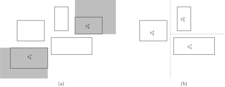
  Figure 2: (a) A size-5 independent set of rectangles in $\mathbb{R}^{2}$. (b) A size-3 independent set.

  A SW quadrant $(-\infty,x]\times(-\infty,y]$ (resp. NE quadrant $[x,\infty)\times[y,\infty)$) is called grid-aligned if $(x,y)$ is one of the $r^{2}$ grid points. Let $\rho_{1}^{*}$ be the smallest grid-aligned SW quadrant containing the SW extension of $v_{1}^{*}$ (in other words, we “round” $v_{1}^{*}$’s corner point upward and rightward to a grid point), and let $\rho_{2}^{*}$ be the smallest grid-aligned NE quadrant containing the NE extension of $v_{2}^{*}$ (in other words, we “round” $v_{2}^{*}$’s corner point downward and leftward to a grid point). The rectangles $\rho_{1}^{*},\rho_{2}^{*},v_{3}^{*},v_{4}^{*},v_{5}^{*}$ are pairwise disjoint (because all edges of $K^{*}$ are high). Among $v_{3}^{*},v_{4}^{*},v_{5}^{*}$, there is a vertical or horizontal line separating one from the other two. W.l.o.g, assume that the separating line is vertical, with $v_{3}^{*}$ to the left, and $v_{4}^{*}$ and $v_{5}^{*}$ to the right, and with $v_{4}^{*}$ below $v_{5}^{*}$. For example, see Figure 2(b).

  Fix a grid-aligned SW quadrant $\rho_{1}$ that contains at least one rectangle $v_{1}\in V^{(1)}$. Fix a grid-aligned NE quadrant $\rho_{2}$ that contains at least one rectangle $v_{2}\in V^{(2)}$, and does not intersect $\rho_{1}$. We find a rectangle $v_{3}\in V^{(3)}$ that does not intersect $\rho_{1}$ and $\rho_{2}$, with the leftmost right side. This can be found by an orthogonal range minimum query in a constant dimension. Next, we find a rectangle $v_{4}\in V^{(4)}$ that does not intersect $\rho_{1}$ and $\rho_{2}$, and is to right of the right side of $v_{3}$, with the lowest top side. Similarly, we find a rectangle $v_{5}\in V^{(5)}$ that does not intersect $\rho_{1}$ and $\rho_{2}$, and is to right of the right side of $v_{3}$, with the highest bottom side. These can also be found by orthogonal range searching. If these two rectangles $v_{4}$ and $v_{5}$ do not intersect, we have found a solution $\{v_{1},\ldots,v_{5}\}$.

  There are $O(r^{2})$ choices of $\rho_{1}$. However, it suffices to consider the minimal grid-aligned SW quadrants $\rho_{1}$ that contain at least one rectangle $v_{1}\in V^{(1)}$, and there are only $O(r)$ choices of such $\rho_{1}$, since the corners of the minimal quadrants form a staircase in the grid. Similarly, it suffices to consider $O(r)$ choices of $\rho_{2}$. Totaling over all $O(r)$ choices of $\rho_{1}$ and $O(r)$ choices of $\rho_{2}$, we have made $O(r^{2})$ range queries on $O(n)$ elements, requiring $\widetilde{O}(n+r^{2})$ time.

We set $r=n^{2/3}$ to equalize $r^{2}$ with $n^{2}/r$. ∎

11 Final Remarks

There are still many variants of these problems that we could address but have not in this paper. We briefly mention the following:

• Counting. For example, the reduction in Theorem 4.6 still works for counting instead of detection. And the algorithm in Theorem 5.1 also seems suitable for counting.

• Minimizing weight. For vertex weights, the reduction in Theorem 4.6 still works, and we can use known results on minimum-weight 3-cycles for sparse graphs [37]. And the algorithm in Theorem 5.1, also seems suitable by using range minimum queries. Kaplan et al. [54] considered finding the minimum-weight $C_{3}$ in a disk intersection graph with edge weights that are Euclidean distances between the centers; our algorithm in Theorem 8.3 also seems adaptable to such edge weights, with some modifications.

• Other geometric objects. Lemmas 4.5 and 5.2 hold not only for line segments but also for triangles or constant-size convex polygons (with more polylogarithmic factors). So, the algorithm in Theorem 5.3 can be generalized to these objects. (One could also consider certain families of curves: Lemma 4.5 holds for pseudo-line segments, and good separators still exist for sparse intersection graphs of curves, but not all techniques for line segments are applicable without increasing the time bounds.)

• Other combinations of patterns and objects. For example, we have not yet considered $I_{4}$ for line-segment intersection graphs, $K_{5}$ for boxes or line segments, $K_{4}$ for 2D translates, etc.

For many of the specific results obtained in this paper, there is room for further improvement in the upper bounds. It would also be desirable to prove conditional lower bounds for more problems in this class.

A main open question is whether subquadratic algorithms exist for $C_{3}$ in range graphs with intrinsic dimension 3 and higher. Our algorithms work in higher dimensions, but the time bound becomes superquadratic (for intrinsic dimension 3, we might still be able to outperform known general $O(n^{\omega})$-time algorithms under the current value of $\omega$, but the time bound would certainly be worse for intrinsic dimension 4). Similarly, the algorithm in Theorem 9.1 becomes superquadratic for dimension 4 and higher.

For one specific open question: can length-3 depth cycles [33] be detected in subquadratic time for a given set of $n$ lines in $\mathbb{R}^{3}$? This problem reduces to finding $C_{3}$ in a range graph with dimension 4.

Appendix A Appendix

A.1 Proof of Lemma 4.3

The proof is based on multi-level cutting trees [36, 7, 63].

Assume that $V$ is divided into two parts $V^{(1)}$ and $V^{(2)}$. Let $n_{1}=|V^{(1)}|$ and $n_{2}=|V^{(2)}|$. Assume that each range $R^{(12)}(v)\subseteq\mathbb{R}^{d}$ is expressed as a fixed Boolean combination of $\ell$ polynomial inequalities $f_{v}(x_{\xi_{1}},x_{\eta_{1}})\geq 0$, …, $f_{v}(x_{\xi_{\ell}},x_{\eta_{\ell}})\geq 0$ (of constant description complexity) over the variables $(x_{1},\ldots,x_{d})$, for a constant $\ell$ and a fixed sequence of indices $\xi_{1},\eta_{1},\ldots,\xi_{\ell},\eta_{\ell}\in[d]$. There are only $O(1)$ number of such index sequences, and $O(1)$ number of Boolean combinations.

Let $b$ be a parameter. By standard results on cuttings [36, 35, 7], we can divide the plane into $b^{2+o(1)}$ cells, such that each cell crosses the boundaries of at most $n_{2}/b$ regions $\{(x_{\xi_{\ell}},x_{\eta_{\ell}})\in\mathbb{R}^{2}:f_{v}(x_{\xi_{\ell}},x_{\eta_{\ell}})\geq 0\}$ over all $v\in V^{(2)}$. The construction takes $O(b^{O(1)}n_{2})$ time. We can further subdivide each cell (by extra vertical cuts) so that each subcell contains at most $n_{1}/b^{2}$ points in $\{(x_{\xi_{\ell}},x_{\eta_{\ell}}):p^{(12)}(u)=(x_{1},\ldots,x_{d}),\ u\in V^{(1)}\}$; the number of cells remains $b^{2+o(1)}$.

For each cell $\gamma$, let $V^{(1)}_{\gamma}=\{u\in V^{(1)}:p^{(12)}(u)=(x_{1},\ldots,x_{d}),\ (x_{\xi_{\ell}},x_{\eta_{\ell}})\in\gamma\}$, let $V^{(2)}_{\gamma}=\{u\in V^{(2)}:\ \mbox{$f_{v}=0$ intersects $\gamma$}\}$, let $Y^{(2)}_{\gamma}=\{u\in V^{(2)}:\ \mbox{$f_{v}>0$ contains $\gamma$}\}$, and let $Z^{(2)}_{\gamma}=\{u\in V^{(2)}:\ \mbox{$f_{v}<0$ contains $\gamma$}\}$.

For each cell $\gamma$, we recursively construct a biclique cover for the subgraph induced by $V^{(1)}_{\gamma}\cup V^{(2)}_{\gamma}$, the subgraph induced by $V^{(1)}_{\gamma}\cup Y^{(2)}_{\gamma}$, and the subgraph induced by $V^{(1)}_{\gamma}\cup Z^{(2)}_{\gamma}$. Note that in second and third recursive calls, $\ell$ decreases by 1 (since the last inequality $f_{v}(x_{\xi_{\ell}},x_{\eta_{\ell}})\geq 0$ has been resolved for $Y^{(2)}_{\gamma}$ and $Z^{(2)}_{\gamma}$). Thus, the biclique cover size satisfies a recurrence of the form

$$S_{\ell}(n_{1},n_{2})\ \leq\ b^{2+o(1)}S_{\ell}(n_{1}/b^{2},n_{2}/b)+b^{2+o(1)}S_{\ell-1}(n_{1},n_{2}),$$ (1)

with trivial base cases $S_{0}(n_{1},n_{2})=O(n_{1}+n_{2})$ and $S_{\ell}(1,n_{2})=O(n_{2})$. Starting from $(n_{1},n_{2})=(n,n)$, the number of subproblems of size $(n_{1},n_{2})=(n/b^{2i},n/b^{i})$ generated by the recursion is bounded by $\min\{(b^{2+o(1)})^{i+\ell},n\}$, and so $S_{\ell}(n,n)=O\left(\sum_{i}\min\{b^{(2+o(1))i},n\}\cdot n/b^{i}\right)\leq O(n^{3/2+\varepsilon})$ for a sufficiently large constant $b$. Moreoever, each vertex in $V^{(1)}$ participates in $O(\log^{\ell}n)=\widetilde{O}(1)$ bicliques. All the properties stated in the lemma thus follow. ∎

A.2 Proof of Lemma 4.4

We modify the proof of Lemma 4.3. Assume that each range $R^{(12)}(v)\subseteq\mathbb{R}^{d}$ is expressed as a fixed Boolean combination of $\ell_{1}$ polynomial inequalities like before. Assume also that each range $R^{(21)}(v)\subseteq\mathbb{R}^{d}$ is similarly expressed as a fixed Boolean combination of $\ell_{2}$ polynomial inequalities. Let $\ell=\ell_{1}+\ell_{2}$. In addition to the earlier recurrence (1) on the biclique cover size, we obtain the symmetric recurrence

$$S_{\ell}(n_{1},n_{2})\ \leq\ b^{2+o(1)}S_{\ell}(n_{1}/b,n_{2}/b^{2})+b^{2+o(1)}S_{\ell-1}(n_{1},n_{2}).$$

Applying the two in succession yields

$$S_{\ell}(n,n)\ \leq\ b^{4+o(1)}S_{\ell}(n/b^{3},n/b^{3})+b^{4+o(1)}S_{\ell-1}(n,n).$$

The number of subproblems of size $(n/b^{3i},n/b^{3i})$ generated by the recursion is at most $(b^{4+o(1)})^{i+\ell}$, and so $S_{\ell}(n,n)=O(\sum_{i:\,b^{3i}\leq n}b^{(4+o(1))i}\cdot n/b^{3i})\leq O(n^{4/3+\varepsilon})$ for a sufficiently large constant $b$. ∎

A.3 Proof of Lemma 4.5

The proof is based on segment trees [34].

For a line segment $s$ and a vertical slab $\sigma$, we say that $s$ is short in $\sigma$ if $s$ has an endpoint strictly inside $\sigma$; we say that $s$ is long in $\sigma$ if $s$ has an endpoint on the left side of $\sigma$ and another endpoint on the right side of $\sigma$.

Suppose that we are given a set $S$ of line segments, all short in a given vertical slab $\sigma$. (Initially, $\sigma$ is the entire plane.) Let $n$ be the number of endpoints strictly inside $\sigma$. Clearly, $|S|\leq n$. We want to construct a biclique cover for the intersection graph of $S$.

Divide $\sigma$ into two subslabs $\sigma_{1}$ and $\sigma_{2}$ each containing $n/2$ endpoints. Fix $i\in\{1,2\}$. Clip the segments of $S$ to $\sigma_{i}$. Let $S_{i}$ be the resulting short segments in $\sigma_{i}$, and $L_{i}$ be the resulting long segments in $\sigma_{i}$. We recursively construct a biclique cover for $S_{i}$. It remains to take cover intersections involving $L_{i}$. The intersection graph of $L_{i}$ is a permutation graph, and there are known straightforward $\widetilde{O}(n)$-time algorithms to color a permutation graph, yielding a proper $k$-coloring if it does not contain $K_{k}$, or outputting a $K_{k}$ otherwise. If a $K_{k}$ is returned, we can stop. Otherwise, take each color class $L_{i}^{(j)}\ (j\in[k])$, which is a disjoint set of long segments. Sort them from bottom to top, and assign such segment $s\in L_{i}^{(j)}$ its rank $p(s)$ in the sorted list. Map each segment $s^{\prime}\in S_{i}\cup L_{i}$ to an interval $I(s^{\prime})$ consisting of the ranks of all segments in $L_{i}^{(j)}$ that intersect $s^{\prime}$. This is indeed an interval, i.e., a contiguous subsequence of integers, and its two endpoints can be found by binary search. We can then compute a biclique cover for $\{(s,s^{\prime})\in L_{i}^{(j)}\times(S_{i}\cup L_{i}):p(s)\in I(s^{\prime})\}$ of size $\widetilde{O}(n)$, e.g., by applying Lemma 4.2 in one dimension.

The total biclique cover size satisfies the recurrence

$$S(n)\leq 2S(n/2)+\widetilde{O}(n),$$

which solves to $\widetilde{O}(n)$. Moreoever, each segment participates in $O(\log n)$ nodes of the recursion, and thus participates in $\widetilde{O}(1)$ bicliques. ∎

Alternatively, one could apply a result from combinatorial geometry by Fox and Pach [48], stating that line-segment intersection graphs avoiding $K_{k}$ can be colored with polylogarithmically many colors (though an algorithmic version of this result would be needed). Then for each pair of colors, one could directly invoke the bichromatic segment intersection algorithm by Chazelle et al. [34] (of which our algorithm above is a modification) to obtain a biclique cover of $\widetilde{O}(n)$ size.

A.4 Proof of Lemma 5.4

We modify the $O(m^{2\omega/(\omega+1)})$-time algorithm of Alon, Yuster, and Zwick [14] or finding 3-cycles.

For a vertex $v\in V^{(1)}\cup V^{(3)}$, call $v$ low if it has at most $\Delta$ neighbors in $V^{(2)}$, and high otherwise. For a vertex $v\in V^{(2)}$, call $v$ low if it has at most $\Delta m^{\prime}/m$ neighbors in $V^{(3)}$, and high otherwise. We seek a 3-cycle $v_{1}^{*}v_{2}^{*}v_{3}^{*}$ with $v_{1}^{*}\in V^{(1)}$, $v_{2}^{*}\in V^{(2)}$, and $v_{3}^{*}\in V^{(3)}$. We consider two cases:

• Case 1: $v_{1}^{*}$ or $v_{3}^{*}$ is low. W.l.o.g., say it is $v_{1}^{*}$. We go through each of the $O(m^{\prime})$ edges $v_{1}v_{3}$ in $V^{(1)}\times V^{(3)}$, and if $v_{1}$ is low, examine each of its $O(\Delta)$ neighbors $v_{2}\in V^{(2)}$ and check whether $v_{1}v_{2}v_{3}$ is a 3-cycle. The running time is $O(m^{\prime}\Delta)$.

• Case 2: $v_{2}^{*}$ is low. We go through each of the $O(m)$ edges $v_{1}v_{2}$ in $V^{(1)}\times V^{(2)}$, and if $v_{2}$ is low, examine each of its $O(\Delta m^{\prime}/m)$ neighbors $v_{3}\in V^{(3)}$ and check whether $v_{1}v_{2}v_{3}$ is a 3-cycle. The running time is $O(m\cdot\Delta m^{\prime}/m)=O(m^{\prime}\Delta)$.

• Case 3: $v_{1}^{*},v_{2}^{*},v_{3}^{*}$ are all high. There are at most $O(m/\Delta)$ high vertices in $V^{(1)}\cup V^{(3)}$, and at most $O(m/(\Delta m^{\prime}/m))=O(m^{2}/(\Delta m^{\prime}))$ high vertices in $V^{(2)}$. We can detect a 3-cycle among the high vertices by rectangular matrix multiplication in $O(M(m/\Delta,m^{2}/(\Delta m^{\prime}),m/\Delta))$ time. ∎

A.5 Proof of Lemma 5.5

We modify the $O(m^{3/2})$-time algorithm of Alon, Yuster, and Zwick [14] for finding 4-cycles.

W.l.o.g., say $m^{\prime}\leq m$. For a vertex $v$ in $V^{(2)}$ (resp. $V^{(4)}$), call $v$ low if it has at most $\Delta$ neighbors in $V^{(3)}$ (resp. $V^{(1)}$), and high otherwise. We seek a 4-cycle $v_{1}^{*}v_{2}^{*}v_{3}^{*}v_{4}^{*}$ with $v_{1}^{*}\in V^{(1)}$, …, $v_{4}^{*}\in V^{(4)}$.

• Case 1: $v_{2}^{*}$ and $v_{4}^{*}$ are both low. We go through each of the $O(m)$ edges $v_{1}v_{2}$ in $V^{(1)}\times V^{(2)}$, and if $v_{2}$ is low, examine each of its $\Delta$ neighbors $v_{3}\in V^{(3)}$ and mark the pair $(v_{1},v_{3})$ red. Similarly, we go through each of the $O(m)$ edges $v_{3}v_{4}$ in $V^{(3)}\times V^{(4)}$, and if $v_{4}$ is low, examine each of its $d$ neighbors $v_{1}\in V^{(1)}$ and mark the pair $(v_{1},v_{3})$ blue. If a pair is marked both red and blue, we have found a 4-cycle $v_{1}v_{2}v_{3}v_{4}$. The running time is $O(m\Delta)$.

• Case 2: $v_{2}^{*}$ or $v_{4}^{*}$ is high. W.l.o.g., say it is $v_{2}^{*}$. There are at most $O(m^{\prime}/\Delta)$ high vertices in $V^{(2)}$. From each such vertex $v$, we run breadth-first search to find a 4-cycle through $v$. The running time is $O(m^{\prime}/\Delta\cdot(m+m^{\prime}))=O(mm^{\prime}/\Delta)$.

Choosing $\Delta=\sqrt{m^{\prime}}$ yields the result. ∎

Note that there might be room for improvement in Lemma 5.5, by modifying Yuster and Zwick’s $O(m^{1.48})$ algorithm for $C_{4}$ in sparse graphs [71] instead of the $O(m^{3/2})$ algorithm. This would require more effort, and the resulting improvement to Theorem 5.6 would likely be very small.

References

- [1] Amir Abboud, Karl Bringmann, Seri Khoury, and Or Zamir. Hardness of approximation in P via short cycle removal: Cycle detection, distance oracles, and beyond. In Proc. 54th Annual ACM Symposium on Theory of Computing (STOC), pages 1487–1500, 2022. doi:10.1145/3519935.3520066.
- [2] Amir Abboud and Virginia Vassilevska Williams. Popular conjectures imply strong lower bounds for dynamic problems. In Proc. 55th Annual IEEE Symposium on Foundations of Computer Science (FOCS), pages 434–443, 2014. doi:10.1109/FOCS.2014.53.
- [3] Pankaj K. Agarwal. Parititoning arrangements of lines II: Applications. Discret. Comput. Geom., 5:533–573, 1990. doi:10.1007/BF02187809.
- [4] Pankaj K. Agarwal. Simplex range searching and its variants: A review. In M. Loebl, J. Nešetril, and R. Thomas, editors, Journey through Discrete Mathematics, pages 1–30. Springer, 2017. URL: http://www.cs.duke.edu/~pankaj/publications/surveys/srs.pdf.
- [5] Pankaj K. Agarwal, Noga Alon, Boris Aronov, and Subhash Suri. Can visibility graphs be represented compactly? Discret. Comput. Geom., 12:347–365, 1994. doi:10.1007/BF02574385.
- [6] Pankaj K. Agarwal, Boris Aronov, Esther Ezra, Matthew J. Katz, and Micha Sharir. Intersection queries for flat semi-algebraic objects in three dimensions and related problems. In Proc. 38th International Symposium on Computational Geometry (SoCG), pages 4:1–4:14, 2022. doi:10.4230/LIPIcs.SoCG.2022.4.
- [7] Pankaj K. Agarwal and Jeff Erickson. Geometric range searching and its relatives. In Advances in Discrete and Computational Geometry, volume 223 of Contemporary Mathematics, pages 1–56. AMS Press, 1999. URL: http://jeffe.cs.illinois.edu/pubs/survey.html.
- [8] Pankaj K. Agarwal and Jirí Matoušek. On range searching with semialgebraic sets. Discret. Comput. Geom., 11:393–418, 1994. doi:10.1007/BF02574015.
- [9] Pankaj K. Agarwal, Mark H. Overmars, and Micha Sharir. Computing maximally separated sets in the plane. SIAM J. Comput., 36(3):815–834, 2006. Preliminary version in SODA 2004. doi:10.1137/S0097539704446591.
- [10] Pankaj K. Agarwal and Micha Sharir. The number of congruent simplices in a point set. Discret. Comput. Geom., 28(2):123–150, 2002. Preliminary version in SoCG 2001. doi:10.1007/s00454-002-0727-x.
- [11] Pankaj K. Agarwal and Marc J. van Kreveld. Connected component and simple polygon intersection searching. Algorithmica, 15(6):626–660, 1996. doi:10.1007/BF01940884.
- [12] Josh Alman and Virginia Vassilevska Williams. A refined laser method and faster matrix multiplication. In Proc. 32nd ACM-SIAM Symposium on Discrete Algorithms (SODA), pages 522–539, 2021. doi:10.1137/1.9781611976465.32.
- [13] Noga Alon, Raphael Yuster, and Uri Zwick. Color-coding. J. ACM, 42(4):844–856, 1995. doi:10.1145/210332.210337.
- [14] Noga Alon, Raphael Yuster, and Uri Zwick. Finding and counting given length cycles. Algorithmica, 17(3):209–223, 1997. doi:10.1007/BF02523189.
- [15] Michael A. Bender and Martin Farach-Colton. The LCA problem revisited. In Proc. 4th Latin American Symposium on Theoretical Informatics (LATIN), pages 88–94, 2000. doi:10.1007/10719839\_9.
- [16] Édouard Bonnet, Sergio Cabello, and Wolfgang Mulzer. Maximum matchings in geometric intersection graphs. In Proc. 37th International Symposium on Theoretical Aspects of Computer Science (STACS), pages 31:1–31:17, 2020. doi:10.4230/LIPIcs.STACS.2020.31.
- [17] Karl Bringmann, Sándor Kisfaludi-Bak, Marvin Künnemann, André Nusser, and Zahra Parsaeian. Towards sub-quadratic diameter computation in geometric intersection graphs. In Proc. 38th International Symposium on Computational Geometry (SoCG), pages 21:1–21:16, 2022. doi:10.4230/LIPIcs.SoCG.2022.21.
- [18] Sergio Cabello and Wolfgang Mulzer. Minimum cuts in geometric intersection graphs. Comput. Geom., 94:101720, 2021. doi:10.1016/j.comgeo.2020.101720.
- [19] Timothy M. Chan. Approximate nearest neighbor queries revisited. Discret. Comput. Geom., 20(3):359–373, 1998. doi:10.1007/PL00009390.
- [20] Timothy M. Chan. Polynomial-time approximation schemes for packing and piercing fat objects. J. Algorithms, 46(2):178–189, 2003. doi:10.1016/S0196-6774(02)00294-8.
- [21] Timothy M. Chan. Dynamic subgraph connectivity with geometric applications. SIAM J. Comput., 36(3):681–694, 2006. Preliminary version in STOC 2002. doi:10.1137/S009753970343912X.
- [22] Timothy M. Chan. Well-separated pair decomposition in linear time? Inf. Process. Lett., 107(5):138–141, 2008. doi:10.1016/j.ipl.2008.02.008.
- [23] Timothy M. Chan. More algorithms for all-pairs shortest paths in weighted graphs. SIAM J. Comput., 39(5):2075–2089, 2010. doi:10.1137/08071990X.
- [24] Timothy M. Chan. A (slightly) faster algorithm for Klee’s measure problem. Comput. Geom., 43(3):243–250, 2010. doi:10.1016/j.comgeo.2009.01.007.
- [25] Timothy M. Chan. Klee’s measure problem made easy. In Proc. 54th IEEE Symposium on Foundations of Computer Science (FOCS), pages 410–419, 2013. doi:10.1109/FOCS.2013.51.
- [26] Timothy M. Chan, Mihai Pǎtraşcu, and Liam Roditty. Dynamic connectivity: Connecting to networks and geometry. SIAM J. Comput., 40(2):333–349, 2011. Preliminary version in FOCS 2008. doi:10.1137/090751670.
- [27] Timothy M. Chan and Dimitrios Skrepetos. All-pairs shortest paths in unit-disk graphs in slightly subquadratic time. In Proc. 27th International Symposium on Algorithms and Computation (ISAAC), pages 24:1–24:13, 2016. doi:10.4230/LIPIcs.ISAAC.2016.24.
- [28] Timothy M. Chan and Dimitrios Skrepetos. All-pairs shortest paths in geometric intersection graphs. J. Comput. Geom., 10(1):27–41, 2019. doi:10.20382/jocg.v10i1a2.
- [29] Timothy M. Chan, Virginia Vassilevska Williams, and Yinzhan Xu. Hardness for triangle problems under even more believable hypotheses: Reductions from Real APSP, Real 3SUM, and OV. In Proc. 54th ACM Symposium on Theory of Computing (STOC), pages 1501–1514, 2022. doi:10.1145/3519935.3520032.
- [30] Timothy M. Chan and Da Wei Zheng. Hopcroft’s problem, log-star shaving, 2D fractional cascading, and decision trees. In Proc. 33rd ACM-SIAM Symposium on Discrete Algorithms (SODA), pages 190–210, 2022. doi:10.1137/1.9781611977073.10.
- [31] Hsien-Chih Chang and Hsueh-I Lu. Computing the girth of a planar graph in linear time. SIAM J. Comput., 42(3):1077–1094, 2013. doi:10.1137/110832033.
- [32] Bernard Chazelle. Cutting hyperplanes for divide-and-conquer. Discret. Comput. Geom., 9:145–158, 1993. doi:10.1007/BF02189314.
- [33] Bernard Chazelle, Herbert Edelsbrunner, Leonidas J. Guibas, Richard Pollack, Raimund Seidel, Micha Sharir, and Jack Snoeyink. Counting and cutting cycles of lines and rods in space. Comput. Geom., 1:305–323, 1991. Preliminary version in FOCS 1990. doi:10.1016/0925-7721(92)90009-H.
- [34] Bernard Chazelle, Herbert Edelsbrunner, Leonidas J. Guibas, and Micha Sharir. Algorithms for bichromatic line-segment problems polyhedral terrains. Algorithmica, 11(2):116–132, 1994. doi:10.1007/BF01182771.
- [35] Bernard Chazelle and Joel Friedman. A deterministic view of random sampling and its use in geometry. Comb., 10(3):229–249, 1990. doi:10.1007/BF02122778.
- [36] Kenneth L. Clarkson. New applications of random sampling in computational geometry. Discret. Comput. Geom., 2:195–222, 1987. doi:10.1007/BF02187879.
- [37] Artur Czumaj and Andrzej Lingas. Finding a heaviest vertex-weighted triangle is not harder than matrix multiplication. SIAM J. Comput., 39(2):431–444, 2009. doi:10.1137/070695149.
- [38] Mina Dalirrooyfard, Thuy Duong Vuong, and Virginia Vassilevska Williams. Graph pattern detection: Hardness for all induced patterns and faster noninduced cycles. SIAM J. Comput., 50(5):1627–1662, 2021. doi:10.1137/20M1335054.
- [39] Mark de Berg, Otfried Cheong, Marc J. van Kreveld, and Mark H. Overmars. Computational Geometry: Algorithms and Applications. Springer, 3rd edition, 2008.
- [40] Friedrich Eisenbrand and Fabrizio Grandoni. On the complexity of fixed parameter clique and dominating set. Theor. Comput. Sci., 326(1-3):57–67, 2004. doi:10.1016/j.tcs.2004.05.009.
- [41] David Eppstein. Subgraph isomorphism in planar graphs and related problems. J. Graph Algorithms Appl., 3(3):1–27, 1999. Preliminary version in SODA 1995. doi:10.7155/jgaa.00014.
- [42] David Eppstein and Jeff Erickson. Iterated nearest neighbors and finding minimal polytopes. Discret. Comput. Geom., 11:321–350, 1994. doi:10.1007/BF02574012.
- [43] Jeff Erickson. On the relative complexities of some geometric problems. In Proc. 7th Canadian Conference on Computational Geometry (CCCG), pages 85–90, 1995. Full version in http://jeffe.cs.illinois.edu/pubs/relative.html.
- [44] Jeff Erickson. New lower bounds for Hopcroft’s problem. Discret. Comput. Geom., 16(4):389–418, 1996. doi:10.1007/BF02712875.
- [45] Esther Ezra and Micha Sharir. Counting and representing intersections among triangles in three dimensions. Comput. Geom., 32(3):196–215, 2005. Preliminary version in SoCG 2004. doi:10.1016/j.comgeo.2005.02.003.
- [46] Tomás Feder and Rajeev Motwani. Clique partitions, graph compression and speeding-up algorithms. J. Comput. Syst. Sci., 51(2):261–272, 1995. doi:10.1006/jcss.1995.1065.
- [47] Jacob Fox and János Pach. Separator theorems and Turán-type results for planar intersection graphs. Adv. Math., 219:1070–1080, 2008.
- [48] Jacob Fox and János Pach. Coloring -free intersection graphs of geometric objects in the plane. Eur. J. Comb., 33(5):853–866, 2012. doi:10.1016/j.ejc.2011.09.021.
- [49] Nóra Frankl and Andrey Kupavskii. On the Erdős-Purdy problem and the Zarankiewitz problem for semialgebraic graphs. CoRR, abs/2112.10245, 2021. arXiv:2112.10245.
- [50] Anka Gajentaan and Mark H. Overmars. On a class of problems in computational geometry. Comput. Geom., 5:165–185, 1995. doi:10.1016/0925-7721(95)00022-2.
- [51] Francois Le Gall and Florent Urrutia. Improved rectangular matrix multiplication using powers of the Coppersmith-Winograd tensor. In Proc. 29th ACM-SIAM Symposium on Discrete Algorithms (SODA), pages 1029–1046, 2018. doi:10.1137/1.9781611975031.67.
- [52] Michael T. Goodrich, Joseph S. B. Mitchell, and Mark W. Orletsky. Approximate geometric pattern matching under rigid motions. IEEE Trans. Pattern Anal. Mach. Intell., 21(4):371–379, 1999. Preliminary version in SoCG 1994. doi:10.1109/34.761267.
- [53] Sariel Har-Peled. Geometric Approximation Algorithms. AMS, 2011.
- [54] Haim Kaplan, Katharina Klost, Wolfgang Mulzer, Liam Roditty, Paul Seiferth, and Micha Sharir. Triangles and girth in disk graphs and transmission graphs. In Proc. 27th European Symposium on Algorithms (ESA), pages 64:1–64:14, 2019. doi:10.4230/LIPIcs.ESA.2019.64.
- [55] Haim Kaplan, Natan Rubin, Micha Sharir, and Elad Verbin. Efficient colored orthogonal range counting. SIAM J. Comput., 38(3):982–1011, 2008. doi:10.1137/070684483.
- [56] Ton Kloks, Dieter Kratsch, and Haiko Müller. Finding and counting small induced subgraphs efficiently. Inf. Process. Lett., 74(3-4):115–121, 2000. doi:10.1016/S0020-0190(00)00047-8.
- [57] Andrea Lincoln, Virginia Vassilevska Williams, and R. Ryan Williams. Tight hardness for shortest cycles and paths in sparse graphs. In Proc. 29th ACM-SIAM Symposium on Discrete Algorithms (SODA), pages 1236–1252, 2018. doi:10.1137/1.9781611975031.80.
- [58] Richard J. Lipton and Robert Endre Tarjan. Applications of a planar separator theorem. SIAM J. Comput., 9(3):615–627, 1980. doi:10.1137/0209046.
- [59] Dániel Marx. Parameterized complexity of independence and domination on geometric graphs. In Proc 2nd International Workshop on Parameterized and Exact Computation (IWPEC), pages 154–165, 2006. doi:10.1007/11847250\_14.
- [60] Dániel Marx and Anastasios Sidiropoulos. The limited blessing of low dimensionality: When is the best possible exponent for -dimensional geometric problems. In Proc. 30th Symposium on Computational Geometry (SoCG), pages 67–76, 2014. doi:10.1145/2582112.2582124.
- [61] Jirí Matoušek. Efficient partition trees. Discret. Comput. Geom., 8:315–334, 1992. doi:10.1007/BF02293051.
- [62] Jirí Matoušek. Range searching with efficient hierarchical cuttings. Discret. Comput. Geom., 10:157–182, 1993. doi:10.1007/BF02573972.
- [63] Jirí Matoušek. Geometric range searching. ACM Comput. Surv., 26(4):421–461, 1994. doi:10.1145/197405.197408.
- [64] Nabil H. Mustafa and János Pach. On the Zarankiewicz problem for intersection hypergraphs. J. Comb. Theory, Ser. A, 141:1–7, 2016. doi:10.1016/j.jcta.2016.02.001.
- [65] Franco P. Preparata. An optimal real-time algorithm for planar convex hulls. Commun. ACM, 22(7):402–405, 1979. doi:10.1145/359131.359132.
- [66] Mihai Pǎtraşcu. Towards polynomial lower bounds for dynamic problems. In Proc. 42nd ACM Symposium on Theory of Computing (STOC), pages 603–610, 2010. doi:10.1145/1806689.1806772.
- [67] Warren D. Smith and Nicholas C. Wormald. Geometric separator theorems & applications. In Proc. 39th IEEE Symposium on Foundations of Computer Science (FOCS), pages 232–243, 1998. doi:10.1109/SFCS.1998.743449.
- [68] Virginia Vassilevska Williams and Yinzhan Xu. Monochromatic triangles, triangle listing and APSP. In Proc. 61st IEEE Symposium on Foundations of Computer Science (FOCS), pages 786–797, 2020. doi:10.1109/FOCS46700.2020.00078.
- [69] Virginia Vassilevska Williams, Joshua R. Wang, Richard Ryan Williams, and Huacheng Yu. Finding four-node subgraphs in triangle time. In Proc. 26th ACM-SIAM Symposium on Discrete Algorithms (SODA), pages 1671–1680, 2015. doi:10.1137/1.9781611973730.111.
- [70] Raphael Yuster and Uri Zwick. Finding even cycles even faster. SIAM J. Discret. Math., 10(2):209–222, 1997. doi:10.1137/S0895480194274133.
- [71] Raphael Yuster and Uri Zwick. Detecting short directed cycles using rectangular matrix multiplication and dynamic programming. In Proc. 15th ACM-SIAM Symposium on Discrete Algorithms (SODA), pages 254–260, 2004. URL: http://dl.acm.org/citation.cfm?id=982792.982828.