A novel GAN-based paradigm for weakly supervised brain tumor segmentation of MR images

Abstract

Segmentation of regions of interest (ROIs) for identifying abnormalities is a leading problem in medical imaging. Using Machine Learning (ML) for this problem generally requires manually annotated ground-truth segmentations, demanding extensive time and resources from radiologists. This work presents a novel weakly supervised approach that utilizes binary image-level labels, which are much simpler to acquire, to effectively segment anomalies in medical Magnetic Resonance (MR) images without ground truth annotations. We train a binary classifier using these labels and use it to derive seeds indicating regions likely and unlikely to contain tumors. These seeds are used to train a generative adversarial network (GAN) that converts cancerous images to healthy variants, which are then used in conjunction with the seeds to train a ML model that generates effective segmentations. This method produces segmentations that achieve Dice coefficients of 0.7903, 0.7868, and 0.7712 on the MICCAI Brain Tumor Segmentation (BraTS) 2020 dataset for the training, validation, and test cohorts respectively. We also propose a weakly supervised means of filtering the segmentations, removing a small subset of poorer segmentations to acquire a large subset of high quality segmentations. The proposed filtering further improves the Dice coefficients to up to 0.8374, 0.8232, and 0.8136 for training, validation, and test, respectively.

1 Introduction

Segmenting anomalies in medical images is a leading problem as it can be used to assist in diagnosis and inform clinical treatment. However, manually segmenting anomalies demands extensive time and resources from radiologists. Training Machine Learning (ML) models for this segmentation task in a supervised manner requires ground-truth segmentations that are also cumbersome to acquire [1, 2]. Furthermore, segmentation models often demand large datasets of annotated medical images, which may not be available for specific contexts such as pediatric cancer [3]. Hence, training ML models with limited or without ground truth segmentation masks is key.

Weakly supervised segmentations facilitates the manual effort by simplifying the required ground truth annotation. This simplification can be done through various means such as using partial annotations [4], bounding boxes [5, 6], circular centroid labels [7], or scribble marks [8]. We opt to use the simplest form of weakly supervised labels; binary image-level labels indicating whether the image has the anomaly of interest or not.

The common approach to weakly supervised segmentation using binary image-level labels is to train a classification model and then using the classification model to infer tumor segmentations. The most popular means of inferring tumor segmentations from classification models is to use class activation maps (CAMs) [9, 10, 11, 12, 13]. There have been other approaches such as classifying patches of an image to form rough segmentations [14] or generating explanation maps using methods such as Local Interpretable Model-Agnostic Explanations (LIME) [15], SHapley Additive exPlanations (SHAP) [16], or Randomized Input Sampling for Explanation (RISE) [17]. However, a more recent approach to weakly supervised segmentation is by using Generative Adversarial Networks (GANs) [18]. Han et al. [19] demonstrated that GANs can generate realistic brain MR images. Their work used a standard GAN approach using a vector from a latent Gaussian space as input to generate brain MR images, demonstrating the potential for realistic brain MR images to be produced from a Gaussian distribution. This idea has been explored for weakly supervised segmentation by generating a healthy version of cancerous brains and then subtracting it from the original image to acquire segmentations [20, 21].

We propose a new methodology for weakly supervised segmentation in 2-dimensional (2D) MR images that only requires binary image-level labels that indicate the presence of glioma, the most common brain tumor in adults, to generate effective segmentations for the glioma. To do so, we use the image-level labels to generate two priors of information. The first are localization seeds acquired from a binary classifier that indicate which regions are likely to contain a tumor and which regions are least likely to contain a tumor. The second is from non-cancerous variations of cancerous MR images that we generate using a new and improved weakly supervised approach incorporating GANs. We also propose a means of improving the segmentation model using the aforementioned binary classifier, given that the classifier has a sufficient understanding of the glioma.

Furthermore, we introduce a weakly supervised measure calculated using the non-cancerous MR image variants that can be used to filter a small subset of poor segmentations, resulting in a large subset of high quality segmentations. Providing high quality segmentations in a weakly supervised manner for a majority of the available datasets significantly reduces the workload for radiologist. In addition, this filtering enables the large subset of kept segmentations to be used for semi-supervised segmentation tasks, which only require a subset of the dataset to have ground truth annotations. Figure 1 visualizes these steps and how the outputs from each step are used in the overall methodology.

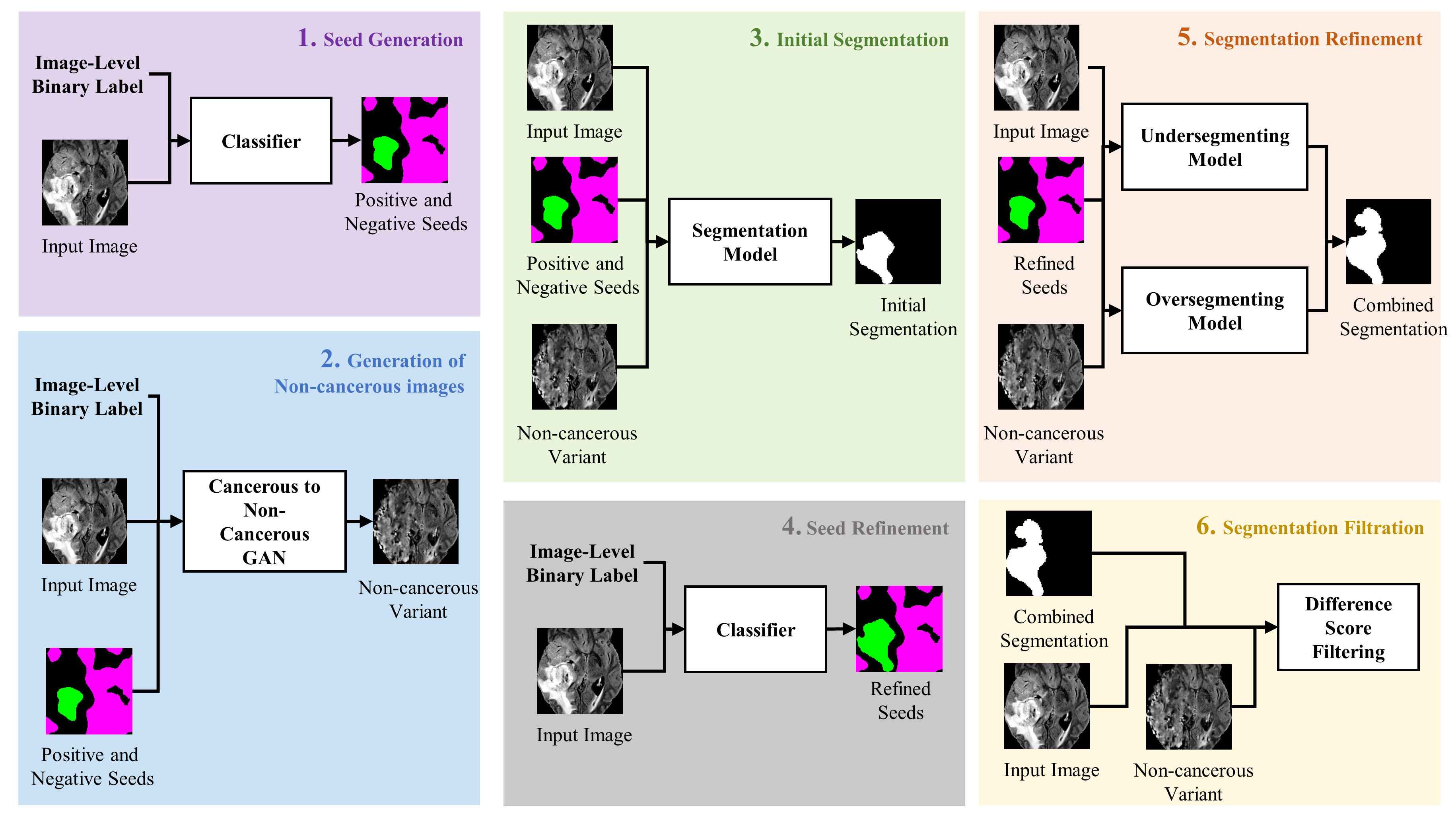
Fig. 1: Block diagram visualizing the overall method

2 Methods

2.1 Seed Generation

We first generate seeds to inform which regions in the images are likely to contain tumors and which regions are unlikely to contain any tumors. These seeds will be used as the primary source of localization information when training the weakly supervised segmentation models.

We define the 2D MR images as $X=\{x^{0},...,x^{k},...,x^{N-1}\}$, $x^{k}\in\mathbb{R}^{c,128,128}$, where $N$ is the number of images and $c$ is the number of channels. We also define the binary-image level labels as $Y=\{y^{0},...,y^{k},...,y^{N-1}\}$, $y^{k}\in\mathbb{R}$ where each slice $y^{k}$ was assigned $0$ if the corresponding image $x^{k}$ was not cancerous, and $1$ otherwise. To generate the seeds, we upsample the spatial dimensions of $X$ from $128\times 128$ to $256\times 256$ using bilinear interpolation and then use the upsampled data with the binary-image level labels to train a classifier model $C()$. We upsample the data because we found that doing so yielded improved seeds compared to using the data with its original spatial dimensions. A quantitative analysis of the effect of upsampling on the seeds is presented in Section 4.1. The predicted classification scores for each image in $X$ are defined as $P=\{p^{0},...,p^{k},...,p^{N-1}\}\in\mathbb{R}\mid 0\leq p^{k}\leq 1$, where $p^{k}>0.5$ indicates that $C()$ predicts $x^{k}$ to be cancerous and $p^{k}\leq 0.5$ indicates that $C()$ predicts $x^{k}$ to be non-cancerous. To reduce the GPU memory load, we only upsampled the data when passed into $C()$, and kept the data at its original spatial dimensions otherwise.

We used the RISE method [17] and normalized the outputs to range $[0,1]$ to acquire the explanation maps $E=\{{e^{0},...,e^{k},...,e^{N-1}}\}\in\mathbb{R}^{N,H,W}$ from $C()$.

Once $E$ is generated, we use it to acquire positive seed regions and negative seed regions. Positive seed regions $S_{+}=\{{s_{+}^{0},...,s_{+}^{k},....,s_{+}^{N-1}}\}\in\mathbb{R}^{N,128,128}$ are binary maps where for each $s_{+}^{k}$, a voxel $(i,j)$ has a value of 1 when the corresponding voxel in $e^{k}$ has a value greater than 0.8 and 0 otherwise. The voxels in the negative seed regions $S_{-}=\{{s_{-}^{0},...,s_{-}^{k},....,s_{-}^{N-1}}\}\in\mathbb{R}^{N,128,128}$ have values of 1 for the corresponding voxels in $E$ that have values less than 0.2 and 0 otherwise. The positive seeds are used to indicate regions in the images that $C()$ believed to contain a tumor and negative seeds are used to indicate regions $C()$ believed to contain no tumor. We threshold by 20% of the maximum and minimum values of each $e^{k}$ to generate the seeds because 20% is the percentile suggested by Zhou et al. [12]. We found the negative seeds from the classifier to be accurate while the positive seeds can contain inaccuracies, depending on what $C()$ interprets to be a tumor. For non-cancerous MR images, we used a positive seed map of all zeros and a negative seed map of all ones. Figure 2 presents examples of positive and negatives seeds.

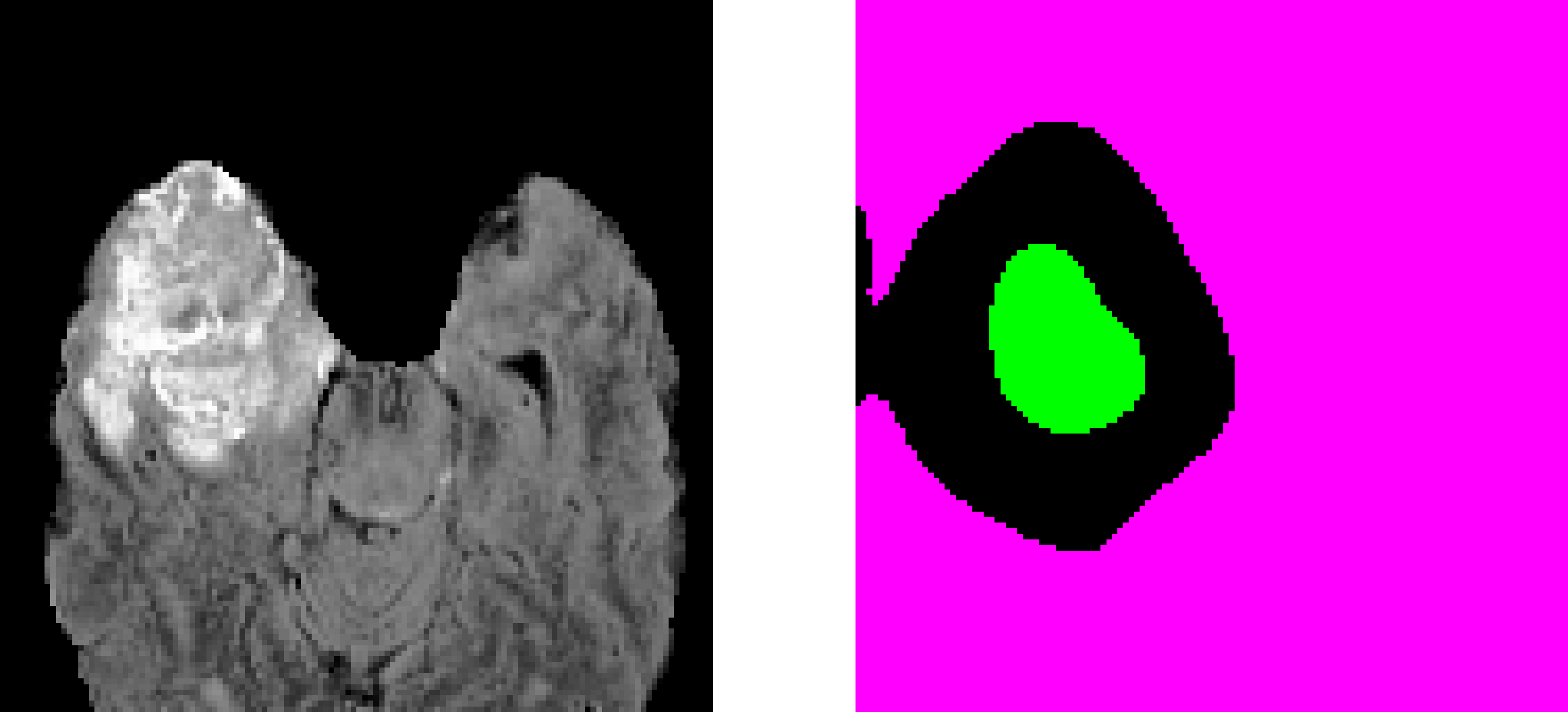
(a) Example from BraTS dataset.

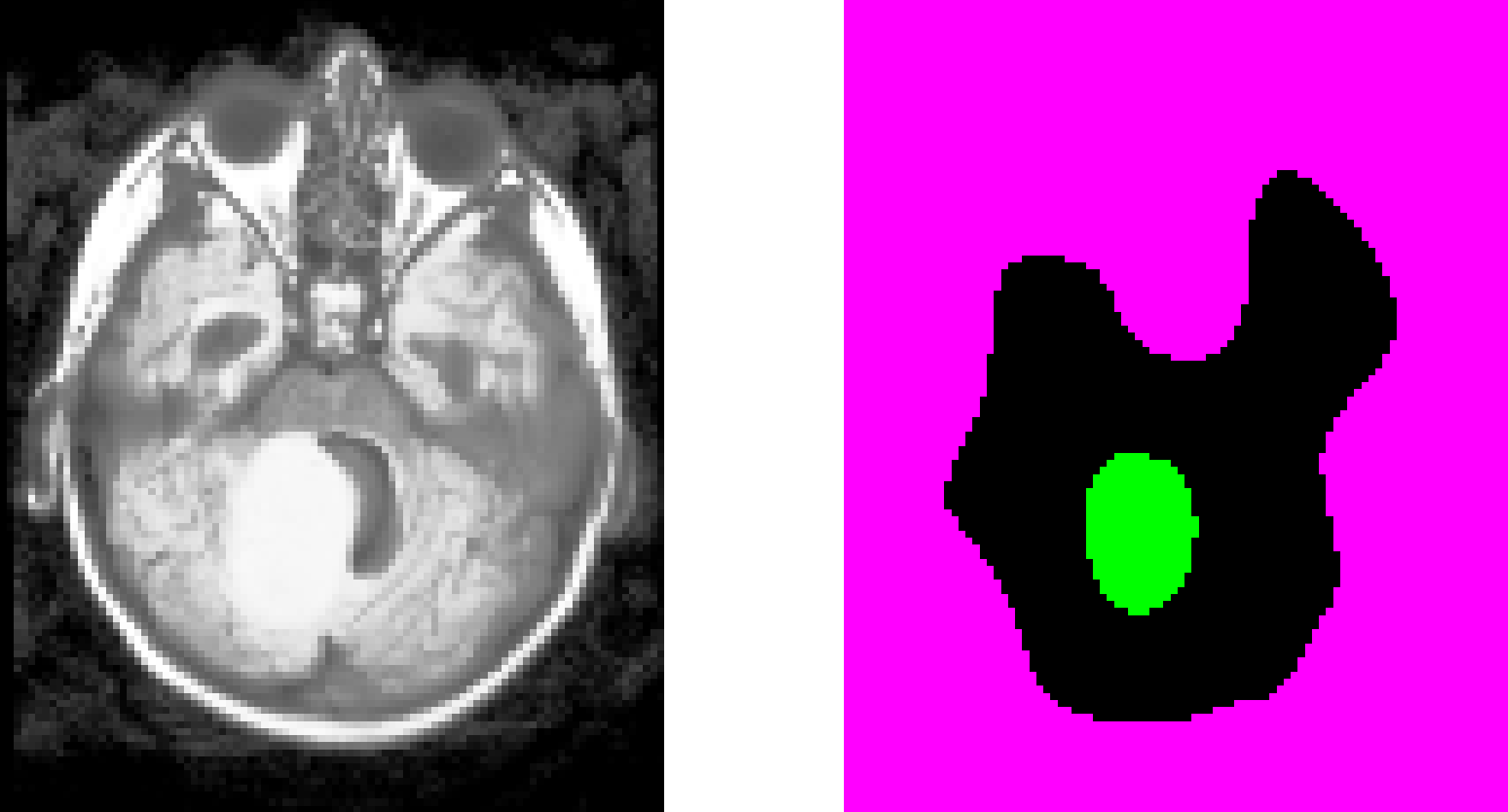
(b) Example from pLGG dataset.

Fig. 2: MR image FLAIR channel (left) and its corresponding positive seeds in green, negative seeds in magenta, and unseeded regions in black (right).

2.2 Generation of Non-cancerous Variations of Cancerous MR Images

Once seeds have been generated, we train a model that receives cancerous images as input and outputs non-cancerous variations of the input images. The non-cancerous variants can be compared to their original to further inform the training of the desired weakly supervised segmentation model. To generate the non-cancerous variants we use an autoencoding U-Net model that consists of an encoder and generator connected by skip connections [22]. The generator is trained individually first to initialize the weights and guide the training toward the desired non-cancerous image outputs.

2.2.1 Generator Training

To generate non-cancerous variations of cancerous MR images, we first define subsets of $X$ from the training cohort, $X_{C}$ which contains all $x^{k}\mid p^{k}>0.5,y^{k}=1$ and $X_{NC}$ which contains all $x^{k}\mid y^{k}=0$. In layman’s terms, $X_{C}$ contains all images that $C()$ correctly believes to be cancerous and $X_{NC}$ contains all images that are non-cancerous according to the ground truth. For $X_{C}$ we use the images with true positive predictions from $C()$ because images resulting with false positives or false negatives from $C()$ are assumed to have poor seeds. The T2-FLAIR channel of $X_{NC}$, defined as $X_{NC,FLAIR}$ is then used to train a generator model $G$ in a DCGAN system that maps the space of unit Gaussian latent vectors to the space of non-cancerous MR images $X_{NC,FLAIR}$. The decision to only use the T2-FLAIR channel for training the DCGAN was also done by Baur et al. [21] and serves to decrease the complexity of the learning task.

A latent vector $z$ sampled from the unit Gaussian space is passed into $G()$ which then outputs a generated image $g$. $g$ is then passed into a discriminator model $D_{0}()$, which is trained to distinguish real and generated images using the binary cross-entropy (BCE) loss function, defined as $L_{D_{0}}$ in Equation 1. $D_{0}()$ is trained in two batches, each of which is of the same size $B$. The first batch consists of real images from $X_{NC,FLAIR}$ and the second batch consists of the generated images. When training DCGANs, the labels are often all $1$ for the batch of real images and all $0$ for the batch of generated images. However, we use one-sided label smoothing which sets our real/generated image labels $y_{0}^{k}$ to $0.9$ for the batch of real images and $0.1$ for the batch of generated images [23]. The one-sided label smoothing is used to prevent the discriminator from becoming too confident in its classifications too quickly, thereby allowing the generator to train effectively. $L_{D_{0}}$ is then used to calculate the loss function of $G()$, $L_{G}$ such that $G()$ learns to trick $D_{0}()$ into discerning generated images as real images. This system is expressed mathematically in equations 1-3. In these equations, the losses are computed over all N but it should be noted that in implementation, minibatches were used, and thus rather than computing the losses over N, they are computed over each batch. For simplicity, the loss equations will be presented as being computed over N.

$$L_{D_{0}} =-\frac{1}{N}\sum_{k=0}^{N-1}\left(y_{0}^{k}\log(D_{0}(x_{\text{in}}^{k}))+(1-y_{0}^{k})\log(1-D_{0}(x_{\text{in}}^{k}))\right),$$ (1)

$$y_{0}^{k} =\begin{cases}0.1,&\text{if}\ x_{\text{in}}^{k}=g\\ 0.9,&\text{if}\ x_{\text{in}}^{k}=x_{NC,FLAIR}^{k}\end{cases}$$

$$g=G(z),z\sim N(0,1)$$ (2)

$$L_{G}=-\frac{1}{N}\sum_{k=0}^{N-1}\log(D_{0}(g))$$ (3)

2.2.2 Full Converting Model Training

Once $G()$ is trained, it is prepended with an encoding model $E()$ using skip connections to form a U-Net model, denoted as $U()$. This U-Net model is then trained in a similar paradigm described in Section 2.2.1 with a few differences. The generated image is no longer acquired from passing a unit Gaussian latent vector to G. Instead, a cancerous image $x_{C,FLAIR}^{k}$ is passed into the U-Net model and the model outputs a non-cancerous version of the image $\hat{x}_{C,FLAIR}^{k}$, which is used as the generated image in the DCGAN system. The architecture of $G()$, $E()$, and $U()$ is visualized in Figure 3. The U-Net model is trained using three loss terms. The first is the adversarial loss $L_{adv}$ which, like $L_{G}$, uses a BCE loss to reward $U()$ for outputting images that a new discriminator $D_{1}()$, trained using $L_{D_{1}}$, classifies as being non-cancerous. The second loss is the reconstruction loss $L_{recon}$ that rewards the U-Net model for generating images that matches the input image at negative seed regions. This has the effect of encouraging the model to keep non-cancerous regions of the cancerous images identical as the negative seed regions correspond to regions likely to contain no tumors. The third loss is a Kullback-Leibler (KL) divergence loss [24], $L_{KL}$ that is applied to the encodings outputted by the final layer of $E()$. This loss encourages the outputs of $E()$, $\hat{z}$ to be within the space of unit Gaussian vectors. Not only does this have a regularizing effect on $U()$ but it also enables $G()$ to be initialized using the weights acquired from the previous training as those weights were trained using unit Gaussian inputs to $G()$. These loss terms are described in Equations 4-10. Examples of cancerous MR images and their non-cancerous variants are presented in Figure 4.

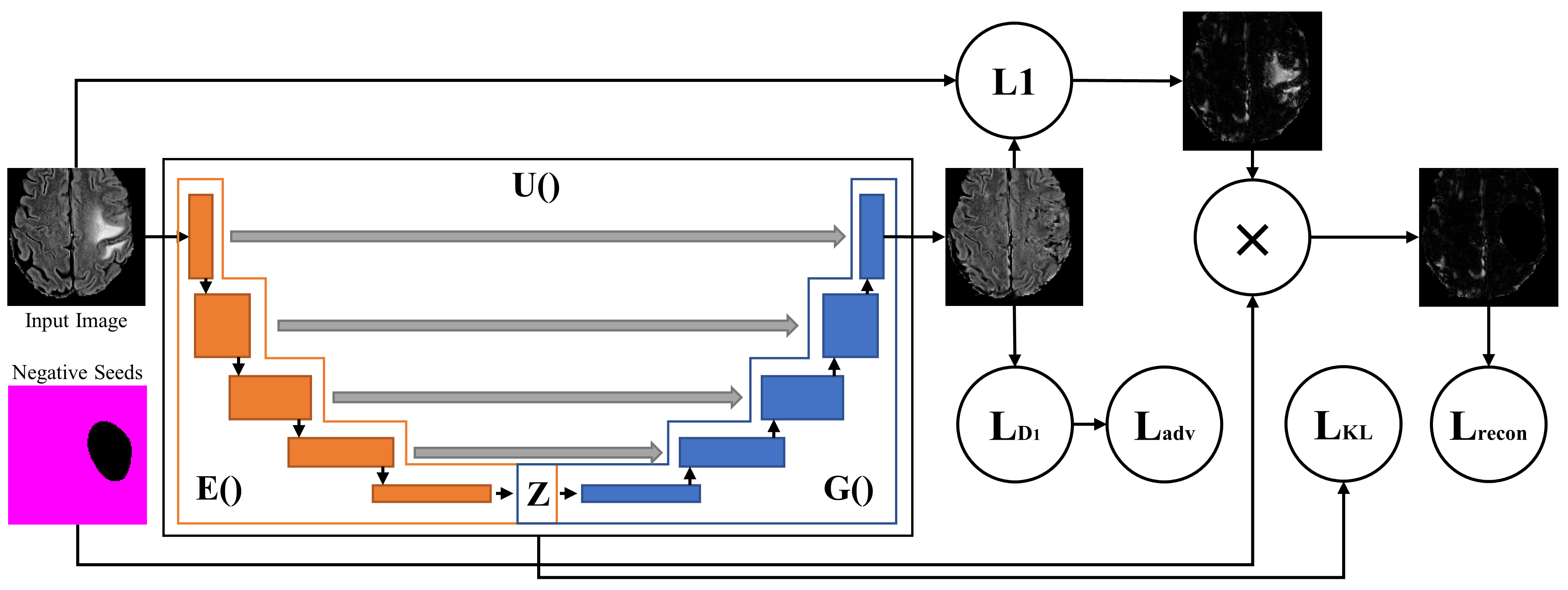
Fig. 3: Architectures for generator $G()$, encoder $E()$, and converting U-Net model $U()$, as well as the calculation of the reconstruction loss $L_{recon}$.

$$\hat{z}^{k}=E(x_{C,FLAIR}^{k})$$ (4)

$$\hat{x}^{k}_{C,FLAIR}=U(x_{C,FLAIR}^{k})$$ (5)

$$L_{D_{1}} =-\frac{1}{N}\sum_{k=0}^{N-1}\left(y_{1}^{k}\log(D_{1}(x_{\text{in}}^{k}))+(1-y_{1}^{k})\log(1-D_{1}(x_{\text{in}}^{k}))\right),$$ (6)

$$y_{1}^{k} =\begin{cases}0.1,&\text{if}\ x_{\text{in}}^{k}=\hat{x}_{C,FLAIR}^{k}\\ 0.9,&\text{if}\ x_{\text{in}}^{k}=x_{NC,FLAIR}^{k}\end{cases}$$

$$L_{adv}= -\frac{1}{N}\sum_{k=0}^{N-1}\log(D_{1}(\hat{x}_{C,FLAIR}^{k}))$$ (7)

$$L_{recon}= \frac{1}{N}\sum_{k=0}^{N-1}\left(\frac{1}{\sum_{i,j}^{H,W}s_{-}^{k}}\sum_{i,j}^{H,W}{s_{-}^{k}}_{i,j}{\lvert x_{C,FLAIR}^{k}-\hat{x}_{C,FLAIR}^{k}\rvert}_{i,j}\right)$$ (8)

$$L_{KL}= -\frac{1}{N}\sum_{k=0}^{N-1}\left(\left(2\log(\sigma_{\hat{z}^{k}})\right)-\sigma_{\hat{z}^{k}}^{2}-\mu_{\hat{z}^{k}}^{2}+1\right)$$ (9)

$$L_{U}=\alpha L_{recon}+\beta L_{adv}+\gamma L_{KL}$$ (10)

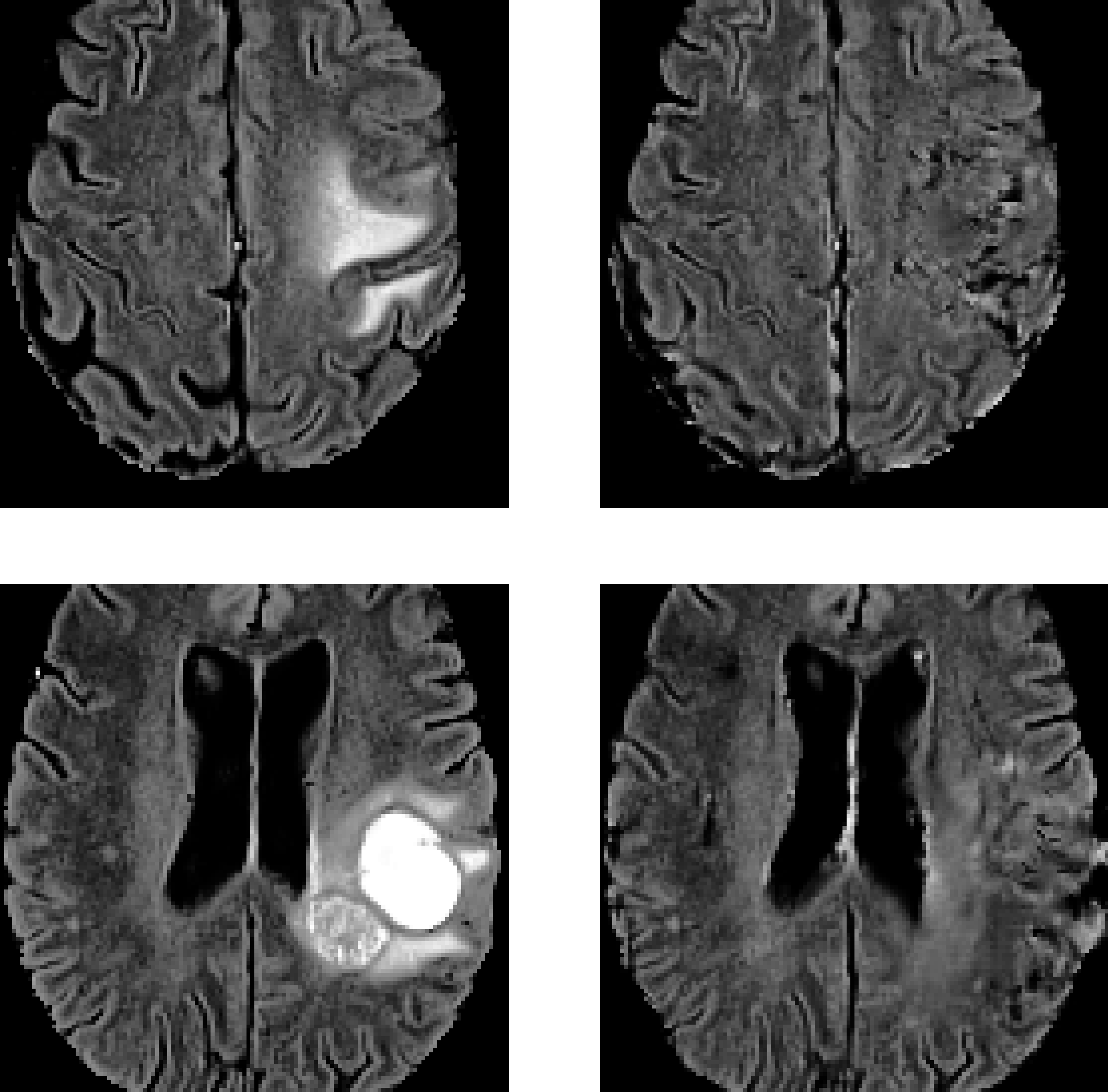
Fig. 4: Examples of MR image FLAIR channel (left) and their generated non-cancerous variant (right).

Note that $\mu_{\hat{z}^{k}}$ and $\sigma_{\hat{z}^{k}}$ are the mean and standard deviation of $\hat{z}^{k}$ respectively. In Equation 10, $\alpha$, $\beta$, and $\gamma$ are weights used to balance the loss terms. We refer to $\alpha$ as the reconstruction scale, $\beta$ as the adversarial scale, and $\gamma$ as the KL scale. When setting the reconstruction scale and adversarial scale to similar values, the adversarial loss tends to dominate the reconstruction loss, resulting with the model tending to generate non-cancerous images that are completely different from the input cancerous images. Thus, the reconstruction scale is required to be significantly greater than the adversarial scale for the model to consistently output non-cancerous variations of the input cancerous images. The KL scale has less of an impact on the outputted images compared to the reconstruction and adversarial scales as this loss is computed using the intermediary output $\hat{z}^{k}$.

Rather than training $U()$ with the whole $X_{C,FLAIR}$, we use a subset of $X_{C,FLAIR}$ whose negative seed regions consist of less than $50\%$ of the image. This is to ensure that when the negative seed region is applied to the input image, a sufficient amount of the image remains for $L_{recon}$.

The decision to train $G()$ and then $U()$ instead of training $U()$ from scratch is inspired by normalizing flow and is used to guide training towards the desired convergence. We found that it can be difficult for the U-Net model to learn to output non-cancerous variations but with the initialization of $G()$ and $L_{KL}$, the training is guided toward outputting non-cancerous MR images, and $L_{recon}$ encourages the outputted images to be variations of the input cancerous MR images.

2.3 Initial Segmentation

To generate segmentations using the generated non-cancerous variations $\hat{X}_{C,FLAIR}$, we use the same U-Net architecture as $U()$ with a new initialization. This new U-Net model, denoted as $S_{0}()$, is trained using three loss terms and all available data $X$ to generate segmentations $M_{0}=\{m_{0},...,m_{0}^{k},...,m_{0}^{N-1}\}$. The first loss term is $L_{seed}$ defined in Equation 12. In this case, we use the positive seeds $S_{+}$ and negative seeds $S_{-}$. This loss uses the available seeds to guide the model toward the desired tumor segmentations. The second loss term is the variation reconstruction loss $L_{var}$ which attempts to minimize the L1 loss between an image $x^{k}$ and its non-cancerous variant $\hat{x}^{k}$ in regions not segmented by $m_{0}^{k}.$ The reasoning behind the reconstruction loss is that cancerous images will differ most from their non-cancerous variants at regions that contain the tumor. Thus, minimizing the L1 loss outside of the segmented regions will encourage the model to segment regions of cancerous images that differ greatly from their non-cancerous counterparts, i.e. tumor locations. For non-cancerous images $X_{NC}$, their non-cancerous variants are considered identical, that is, $X_{NC,FLAIR}=\hat{X}_{NC,FLAIR}$. As the output segmentations cannot be converted to binary segmentations in a differentiable manner, we multiply the voxel-wise L1 loss map between $x_{FLAIR}^{k}$ and $\hat{x}_{FLAIR}^{k}$ by $1-m_{0}^{k}$, as the seed loss will encourage the model’s outputs to be close to 0 or 1 due to $S_{+}$ and $S_{-}$ being binary. Although non-cancerous variations are not sufficient for segmenting on their own, $L_{var}$ enables them to inform the model on how tumors should be segmented. The final loss term is a size loss $L_{size}$ that simply encourages the model to minimize the sum of its outputs. As the seed loss encourages outputs close to 0 or 1, the size loss encourages the model to have tight segmentations around the boundaries of the tumors, as this is the only way to minimize the size loss without compromising the other loss terms. This system is visualized in Figure 5 and these loss terms are expressed in Equations 11-15.

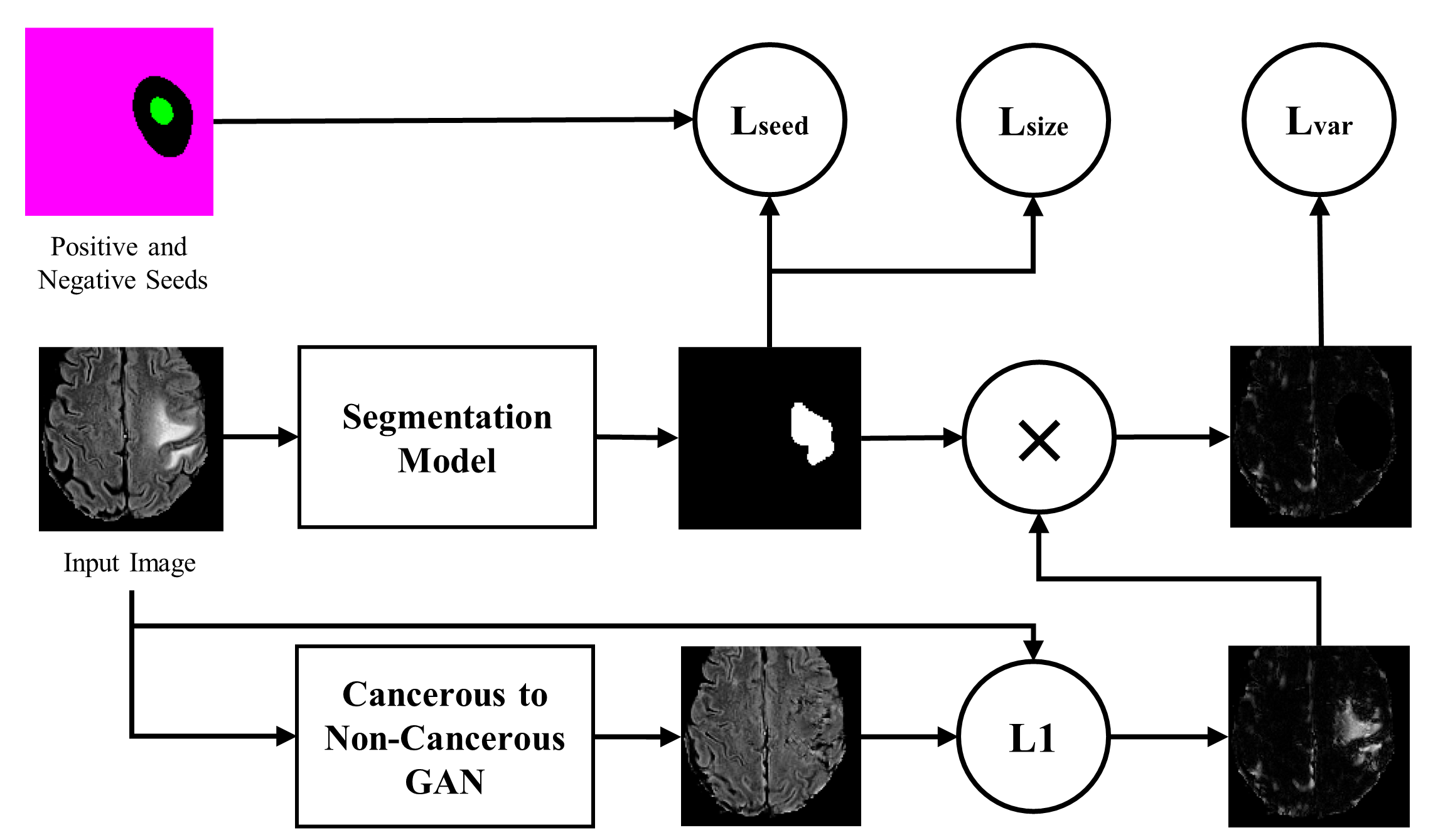
Fig. 5: System for training the segmentation model using the seed loss, variation reconstruction loss, and size loss.

$$m_{0}^{k} =S_{0}(x^{k})$$ (11)

$$L_{seed}=\frac{1}{N}\sum_{k=0}^{N-1}\left(-\frac{1}{\sum_{C\in[+,-]}\lvert{s_{C}^{k}}\rvert}\sum_{C\in[+,-]}\sum_{i,j\in s^{k}_{C}}\log\left({m_{0}^{k}}_{i,j}\right)\right)$$ (12)

$$L_{var}= \frac{1}{N}\sum_{k=0}^{N-1}\left(\frac{1}{\sum_{i,j}^{H,W}s_{-}^{k}}\sum_{i,j}^{H,W}{s_{-}^{k}}_{i,j}{\lvert x_{FLAIR}^{k}-\hat{x}_{FLAIR}^{k}\rvert}_{i,j}\right)$$ (13)

$$L_{size}= \frac{1}{N}\sum_{k=0}^{N-1}\left(\frac{1}{HW}\sum_{i,j}^{H,W}{m_{0}^{k}}_{i,j}\right)$$ (14)

$$L_{M_{0}}=\delta L_{seed}+\epsilon L_{var}+\zeta L_{size}$$ (15)

$\delta$, $\epsilon$, and $\zeta$ from Equation 15 are weights to balance the loss terms for $L_{M_{0}}$. The weight for $L_{size}$ is set to the lowest value between the three weights because we do not want the size loss to overpower the other losses and begin excessively shrinking the segmentations or decreasing the intensity values of the segmented voxels. Since the non-cancerous variations do not always differ from their original counterparts solely at the tumor locations, we rely on the seeds more than the generated images. Thus, the weight for $L_{seed}$ is greater than the weight for $L_{var}$.

When acquiring segmentations from $S_{0}()$ for evaluation, we assume that the images predicted by $C()$ to have no tumor have segmentation maps consisting of all zero values.

2.4 Seed and Segmentation Refinement

One limitation with the approach presented in Section 2.3 is that it is highly reliant on the seeds. The negative seeds are reliable enough such that they can be considered to be accurate but many of the positive seeds are flawed, obfuscating some of the output segmentations by segmenting random patches without tumors.

To resolve this, we first refine the seeds by acquiring new positive seeds. To acquire these new positive seeds, we binarize the segmentations $M_{0}$ corresponding to images in $X_{C}$ by thresholding values above $0.5$ to $1$ and values below or equal to $0.5$ to $0$. If $m_{0}^{k}$ outputs multiple separate segmentations, we extract each separate segmentation, determined using connected-component labeling, and apply each separate one individually. We denote these altered initial segmentations as $\hat{M}_{0}$. Each segmentation in $\hat{M}_{0}$ is then dilated using disks with radii ranging from $1-5$ pixels to slightly increase their size by varying amounts. The inverse of the segmentation at each dilation radius is then multiplied by the corresponding image of the segmentation from $X_{C}$ and input to $C()$. If the average output of $C()$ across all dilation radii for a segmentation $\hat{m}_{0}^{k}$ is less than $0.5$, we assume that the corresponding initial segmentation ($\hat{M}_{0}$) sufficiently covers the tumor and select it as the new positive seed. The use of multiple dilation radii ensures that the $\hat{M}_{0}$ segments a tumor, as correct segmentations should mask tumors and consistently decrease the classifier’s prediction across all radii. We also place each image in $X_{C}$ that had a segmentation considered valid by this process into a new subset of data $X_{C,r}$ as we are not interested in training using cancerous data with unreliable seeds. The new positive seeds for non-cancerous images are simply all zeros, as they were before. These new positive seeds are defined as $S_{+,r}$. We keep the negative seeds unaltered but define $S_{-,r}$ as the negative seeds corresponding to $X_{C,r}$ and $X_{NC}$. An example of how a selected positive seed compares with the initial seed is presented in Figure 6. An example of a segmentation that was not selected as a new positive seed is presented in Figure 7. While these new seeds only keep segmentations that cover a majority of the tumor, they remove segmentations that are not localized to the tumor due to following initial positive seeds that were not localized to the tumors.

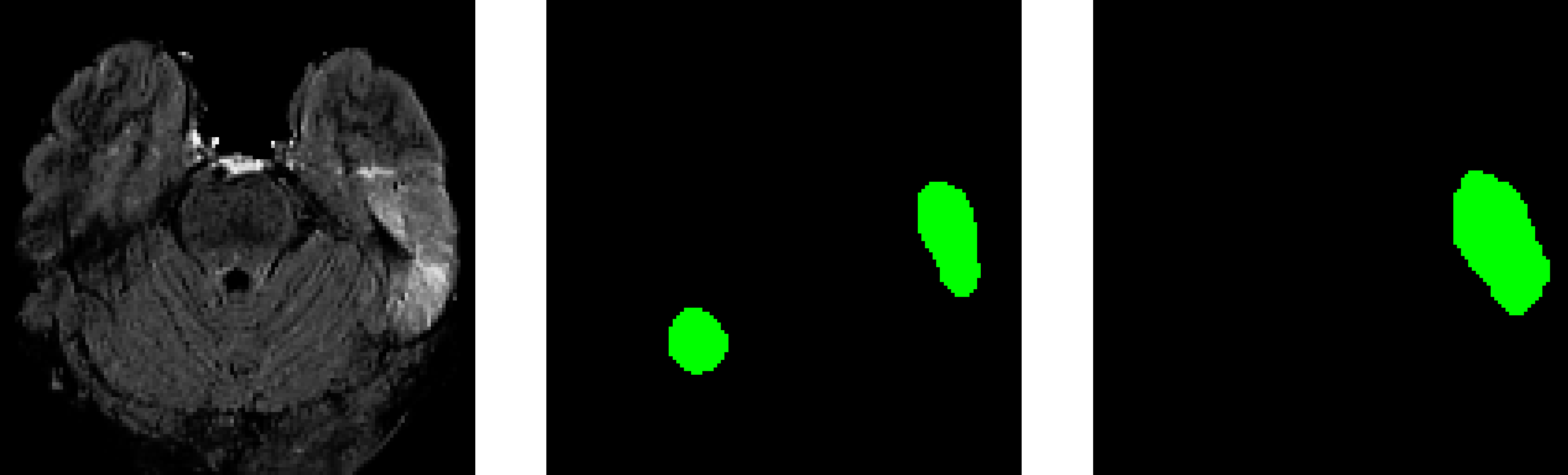
Fig. 6: An example of an MR image FLAIR channel (left), its initial segmentation (middle), and its updated positive seed (right).

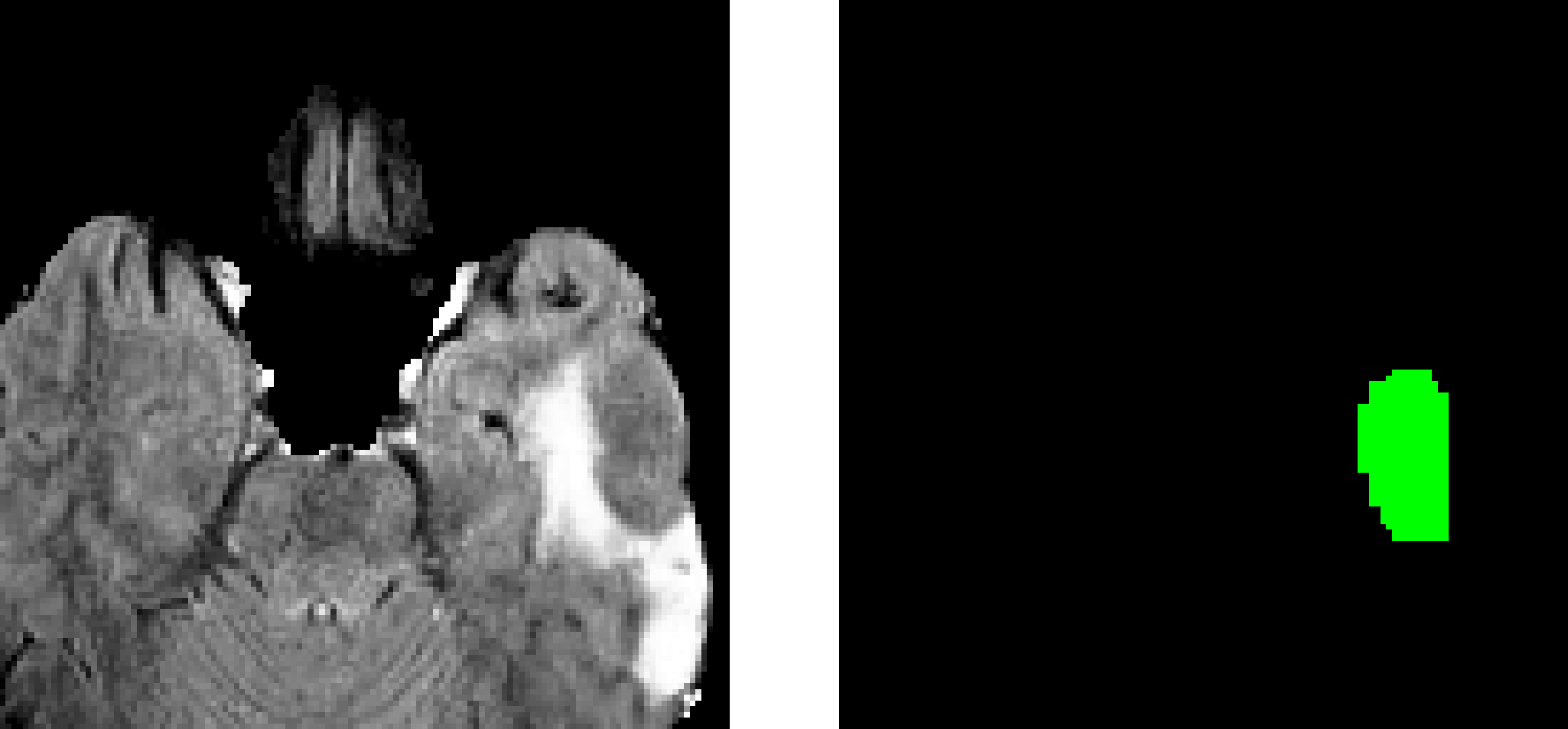
Fig. 7: An example of an MR image FLAIR channel (left) and its initial seed that was not selected as a updated positive seed (right).

These new seeds are then used to perform the method presented in Section 2.3 again using the new positive seeds. A new seed loss, denoted as $L_{seed,r}$ accounting for the new positive seeds $S_{+,r}$ is presented in Equation 16. However, instead of training one model, two models are trained using the new seeds.

$$L_{seed,r}=\frac{1}{N}\sum_{k=0}^{N-1}\left(-\frac{1}{\sum_{C\in[+,-]}\lvert{s_{C,r}^{k}}\rvert}\sum_{C\in[+,-]}\sum_{i,j\in s^{k}_{C,r}}\log\left({m_{0}^{k}}_{i,j}\right)\right)$$ (16)

One model is trained using both the cancerous images $X_{C,r}$ and non-cancerous images $X_{NC}$ while the other is trained solely using cancerous images $X_{C,r}$. In a weakly supervised context such as this one, we found that training with both the cancerous and non-cancerous images results in an undersegmenting model while training with the cancerous images only leads to an oversegmenting model. This is because the undersegmenting model attempts to output empty segmentations for non-cancerous images and thus it might fail to segment difficult-to-discern tumors or smaller tumors, while the oversegmenting model assumes every input is cancerous and will better segment the difficult to discern tumors but can segment regions without tumors as it has not been trained with non-cancerous images.

We now present a simple approach to using $C()$, the undersegmenting model which we denote as $S_{US}()$, and the oversegmenting model which we denote as $S_{OS}()$, to produce the final segmentations. We first pass a brain MR image $x^{k}$ to $C()$ and acquire a classification score $p^{k}$. If $p^{k}<=0.5$, then we use an empty segmention as its segmentation as we assume the image to be non-cancerous. If $p^{k}>0.5$, we pass $x^{k}$ to $S_{US}()$ and $S_{OS}()$ to generate candidate segmentations $m_{US}^{k}$ and $m_{OS}^{k}$. We then calculate a weight $w^{k}$ and use it to combine $m_{US}^{k}$ and $m_{OS}^{k}$ into a segmentation map $m_{1}^{k}$, as shown in Equations 17-18. We then binarize $m_{1}^{k}$ by setting all values greater than $0.5$ to $1$ and all other values to $0$, resulting in a final segmentation $m_{2}^{k}$.

$$w^{k}=2(p^{k}-0.5)$$ (17)

$$m_{1}^{k}=w^{k}m_{OS}^{k}+\left(1-w^{k}\right)m_{US}^{k}$$ (18)

2.5 Weakly Supervised Filtering of Poor Segmentations

One limitation of the proposed method is its heavy reliance on the trained classifier $C()$. To offset the importance of the classifier, we propose a means of identifying poorer segmentations without directly using the classifier. To do so, we calculate a difference score $d^{k}$ for each segmentation $m_{2}^{k}$. The difference score is measured by calculating the mean absolute difference between an image $x^{k}$ and its non-cancerous variant $\hat{x}^{k}$ in the segmentation region defined by $m_{2}^{k}$, as expressed in Equation 19. This difference score measures how much of a segmented area is altered between an image and its non-cancerous variant.

$$d^{k}=\begin{cases}\frac{1}{\mid m_{2}^{k}\mid}\sum_{i,j\in m_{2}^{k}}\mid x^{k}_{FLAIR_{i,j}}-\hat{x}_{FLAIR_{i,j}}^{k}\mid,&\text{if}\ \mid m_{2}^{k}\mid>0\\ 1,&\text{otherwise}\end{cases}$$ (19)

Once the difference score is calculated, segmentations can be deemed poor based on how low their difference score is. Choosing the threshold to filter segmentations is a trade-off between the number of segmentations filtered and the mean quality of the kept segmentations, measured using the Dice coefficient. With a higher threshold, more segmentations are filtered out but the mean Dice of the remaining segmentations improves until an asymptotic limit.

3 Experiments

We evaluate our proposed weakly supervised on two brain MR imaging datasets. The first is the popular open source MICCAI Brain Tumor Segmentation (BraTS) 2020 dataset [25, 26, 27, 28, 29] and the second is an internal pediatric low-grade glioma (pLGG) dataset. For training, we preprocess the images to spatial dimensions of $128\times 128$ but to evaluate the performance of the trained models, we segment the whole 2D MR images. To do so, we split the whole 2D MR images into patches with spatial dimensions of $128\times 128$. Each patch is then passed to the classifier $C()$ and if the input patch is classified as non-cancerous, the patch is assigned an empty segmentation probability map. The segmentation model is then applied to each patch deemed to be cancerous by the classifier. The segmentation probability maps for all patches are then reconstructed to a whole image segmentation probability map, with the probability maps being averaged at regions with overlapping patches, before being binarized by setting all values greater than $0.5$ to $1$ and all other values to $0$.

3.1 Data

3.1.1 MICCAI Brain Tumor Segmentation 2020 Dataset

To form the primary target dataset, the native (T1-weighted), post-contrast T1-weighted, T2-weighted, and T2 Fluid Attenuated Inversion Recovery (T2-FLAIR) volumes from the open source BraTS 2020 dataset containing HGG and LGG tumors were first randomly divided into training, validation and test cohorts using 80/10/10 splits. Each volume was then preprocessed by first cropping each image and segmentation map using the smallest bounding box which contained the brain, clipping all non-zero intensity values to the 1 and 99 percentiles, normalizing the cropped volumes using min-max scaling, and then randomly cropping and padding the volumes to fixed patches of size $128\times 128$ along the coronal and sagittal axes, as done by Henry et al. [30] in their work with BraTS datasets. The volumes and segmentation maps were then split into axial slices to form sets of stacked 2D images with 4 channels $x^{k}\in\mathbb{R}^{4,H,W}$, forming the set $X=\{x^{0},...,x^{k},...,x^{N-1}\}$, where $N$ is the number of images in the dataset, and both $H$ and $W$ are $128$ when training. Slices with more than 50% of voxels equal to zero were removed from $X$. Only the training set of the BraTS dataset was used because it is the only one with publicly available ground truths.

The dataset offers ground-truth segmentations which have to be converted to binary labels to match the weakly supervised task. The segmentations are provided as values that are 0 where there are no tumors and an integer between 1-4 depending on the region of the tumor in which a voxel is located. As this work focuses solely on segmenting the whole tumor, a new set of ground truths $Y=\{y^{0},...,y^{k},...,y^{N-1}\}$, $y^{k}\in\mathbb{R}$ is defined, where for each slice $y^{k}$ was assigned $0$ if the corresponding segmentations were empty, and $1$ otherwise.

To account for images with tumors that are too small to be effectively segmented, small labels were removed using morphological erosion. Erosion removes pixels on object boundaries, removing the small tumor labels and shrinking other tumor labels. Erosion is commonly followed by dilation, which restores shrunken labels back to their original size, but since we are only concerned with the presence of a tumor, dilation is unnecessary. To effectively perform erosion, the segmentation labels were binarized first, with values greater than 0 set to 1. To demonstrate the need for erosion to set small tumor labels as no tumor in the binary classification, Figure 8 presents an MR image with a tumor that is not removed by erosion and its corresponding ground truth segmentation and Figure 9 presents an image with a tumor that is removed by erosion and its corresponding ground truth segmentation.

Fig. 8: MR image with tumor that is not removed by erosion (left) and its corresponding ground truth segmentation before erosion (right).

Fig. 9: MR image with tumor that is removed by erosion (left) and its corresponding ground truth segmentation before erosion (right).

369 patient volumes from the BraTS 2020 training set were split into 295, 37, and 37 volumes for the training, validation, and test cohorts, respectively. After splitting the volumes into 2D images, the first 30 and last 30 slices of each volume were removed, as done by Han et al. [19] because these slices lack useful information. The training, validation, and test cohorts had 24635, 3052, and 3110 stacked 2D images, respectively. The number of images in each class for each cohort are presented in Table 1.

3.1.2 Internal Pediatric Low-Grade Glioma Dataset

We also evaluated our proposed method using an internal dataset from the Hospital for Sick Children consisting of 340 T2-FLAIR patient volumes containing pLGG. This retrospective study was approved by the research ethics board of The Hospital for Sick Children (Toronto, Ontario, Canada). Due to the retrospective nature of the study, informed consent was waived by the local research ethics board. This dataset consisting of 340 patient volumes is the largest pLGG dataset in the world and includes patients ranging from 0 to 18 years old that were identified using the electronic health record database of the hospital from January 2000 to December 2018. There were two main differences in the preprocessing performed for this secondary target dataset compared to the preprocessing done for the BraTS dataset. The first difference was that the volumes from the pLGG dataset were unable to be cropped to their smallest bounding box due to noise in the image backgrounds. Instead, the volumes were downsampled by a factor of 2 from $240\times 240$ to $120\times 120$ along the coronal and sagittal axes so that randomly cropping and padding the volumes to patches of size $128\times 128$ along the coronal and sagittal axes would not remove a majority of the volumes. Given that only the FLAIR channel was available, the second difference was that the volumes for this dataset were split into axial slices forming stacked 2D images with 1 channel instead of 4 channels, resulting in the dataset consisting of images $X=\{x^{0},...,x^{k},...,x^{N-1}\}$, $x^{k}\in\mathbb{R}^{1,H,W}$, where $N$ is the number of images in the dataset, and both $H$ and $W$ are $128$ when training.

After preprocessing, the 340 pLGG patient volumes were split into 272, 34, and 34 volumes for the training, validation, and test cohorts respectively. After splitting into 2D images and removing the first and last 30 slices from each volume, the training, validation and test cohorts had 24499, 3204, and 3205 stacked 2D images respectively. The number of images in each class for each cohort are presented in Table 1.

Table 1: Number of images in each class for each cohort.

Dataset	Cohort	No Tumor (0)	Tumor (1)	Total
	Training	7653	16982	24635
BraTS	Validation	847	2205	3052
	Test	1022	2088	3110
	Training	16298	8201	24499
pLGG	Validation	2203	1001	3204
	Test	2148	1057	3205

3.2 Implementation

All models and training loops were implemented using Python 3.9 and PyTorch 1.12 [31].

The classifier model $C()$ was implemented using a VGG16 architecture with batch normalization. The first layer was altered to receive 4 channel inputs and the final linear layer was altered to output 1 feature before being passed to a sigmoid activation function. This model was trained with a binary cross-entropy loss function for 100 epochs using a batch size of 32, a weight decay of 0.1, and an Adam optimizer with $\beta_{1}=0.9$ and $\beta_{2}=0.999$. The learning rate was initially set to $510-6$ and decreased by a factor of 10 each time the learning rate decreased by a change less than $110-4$. Class weights were applied so that cancerous and non-cancerous images were input equally during training.

$G()$ was trained using a generator with 6 blocks, each of which consisted of a transposed convolution, a batch normalization layer, and a ReLU activation function. The final block did not use a batch normalization layer and used a sigmoid activation function instead of a ReLU activation function. When training $G()$, the initial learning rate for both the generator and the discriminator was $210-4$, which was decreased by a factor of 2 every 50 epochs. $G()$ and its discriminator were trained for 100 epochs using a batch size of 32 and Adam optimizers with $\beta_{1}=0.5$ and $\beta_{2}=0.999$.

The remaining models were trained for 200 epochs with a batch size of 32 and used initial learning rates of $210-4$ that decreased by a factor of 2 every 50 epochs.

All discriminators used a 6 block encoding model, with each block consisting of a convolution, batch normalization layer, and a leaky ReLU activation function with a negative slope of 0.2. The first and final blocks did not use batch normalization, and the final layer used a sigmoid activation function instead of leaky ReLU.

All U-Net models consisted of encoding architecture equivalent to that of the discriminator except the final layer outputted a vector of 100 elements instead of a scalar value. The decoding architecture of the U-Net models were equivalent to that of $G()$. The skip connections consisted of two convolution layer and ReLU activation function blocks. The first received the encoding input, whose output was concatenated with the decoding input and passed into the second block.

When training the cancerous to non-cancerous conversion models using the BraTS dataset, we set the reconstruction scale $\alpha=10$, adversarial scale $\beta=0.05$, and the KL scale $\gamma=1$. For the pLGG dataset, these hyperparameters were set to $\alpha=50$, $\beta=0.05$, $\gamma=1$.

When training the segmentation models using the BraTS dataset, we chose the weights for $L_{seed}$ ($\delta$), $L_{var}$ ($\epsilon$), and $L_{size}$ ($\zeta$) to be $\delta=4$, $\epsilon=1$, and $\zeta=0.25$. For the pLGG dataset, we used $\delta=4$, $\epsilon=1$, and $\zeta=0.2$.

The changes in hyperparameters indicate that the relative difference between the reconstruction scale and adversarial scale, as well as the weight of the size loss may need to be tuned depending on the dataset.

$L_{size}$ is set to the lowest value because we do not want the size loss to overpower the other losses and begin excessively shrinking the segmentations or decreasing the intensity values of the segmented voxels. Since the non-cancerous variations do not always differ from their original counterparts solely at the tumor locations, we rely on the seeds more than the generated images. Thus, the weight for $L_{seed}$ is greater than the weight for $L_{var}$.

4 Results

4.1 Classifier

We first evaluate the classifier model and compare the effect of using a classifier trained using images from the BraTS dataset with the initial spatial dimensions of $128\times 128$ to a classifier trained using data upsampled to spatial dimensions of $256\times 256$.

The area under the ROC curve (AUC), sensitivity, and specificity of the classifier trained without upsampled BraTS inputs and the classifier trained with upsampled BraTS inputs are presented in Table 2. It can be seen in these results that the performance of the two classifiers in the classification metrics are extremely similar. Table 2 also presents the performance of the classifier trained using the pLGG dataset. To be consistent with the dimensions used for the BraTS dataset, we also upsampled the inputs to the classifier from $128\times 128$ to $256\times 256$ when using the pLGG dataset.

Table 2: AUC, sensitivity, and specificity for classifier trained with $128\times 128$ BraTS images, $256\times 256$ BraTS images, and $256\times 256$ pLGG images on all cohorts.

Dataset	Classifier Input Dimensions	AUC			Sensitivity			Specificity
		Training	Validation	Test	Training	Validation	Test	Training	Validation	Test
BraTS	$128\times 128$	0.9999	0.9964	0.9888	0.9995	0.9386	0.9305	0.9998	0.9982	0.9650
	$256\times 256$	0.9999	0.9983	0.9879	0.9991	0.9457	0.9188	0.9997	0.9946	0.9674
pLGG	$128\times 128$	0.9999	0.9809	0.9925	0.9990	0.9846	0.9805	0.9992	0.8951	0.9309
	$256\times 256$	0.9999	0.9841	0.9869	0.9995	0.9891	0.9884	0.9990	0.8991	0.9243

Table 3 presents a simple metric we refer to as the overlap metric to quantitatively compare the initial seeds produced from each classifier. The overlap metric simply refers to the percentage of the positive seed voxels that overlap with the ground truth segmentations and the percentage of the negative seed voxels that do not overlap with the ground truth segmentations. A higher value indicates better seeds. The overlap metric was not used at any point during the actual computation of the segmentations, and simply serves to better interpret observed behavior and results.

Table 3: Overlap metric for a classifier trained with $128\times 128$ BraTS images, a classifier trained with $256\times 256$ BraTS images, and a classifier trained with $256\times 256$ pLGG images on all cohorts.

Dataset	Classifier Input Dimensions	Initial Positive Seeds			Negative Seeds
		Training	Validation	Test	Training	Validation	Test
BraTS	$128\times 128$	0.6296	0.5830	0.5502	0.9910	0.9948	0.9951
	$\mathbf{256\times 256}$	0.7637	0.8294	0.8179	0.9956	0.9968	0.9981
pLGG	$128\times 128$	0.1407	0.1342	0.1019	0.9891	0.9941	0.9931
	$\mathbf{256\times 256}$	0.3634	0.3048	0.3228	0.9996	0.9999	0.9992

It can be seen that despite the similar AUC, sensitivity, and specificity of the classifierst traijned using the BraTS dataset, the classifier with upsampled inputs outperforms the classifier without upsampled inputs in the overlap metric for both positive and negative seeds, as well as across all cohorts. These results indicate that for generating seeds from classifier models, having larger input spatial dimensions can improve the understanding that a classifier has in identifying the desired anomaly, thereby improving the generated seeds.

It should be noted that the overlap scores of the positive seeds for the pLGG dataset are significantly worse than the positive seed overlap scores for the BraTS dataset. We attribute the difference in overlap scores to the lack of T1-weighted, post-contrast T1-weighted, and T2-weighted images in the pLGG dataset. Lacking these images in the pLGG dataset reduced the amount of information available to correlate tumors to the correct classification, resulting with a pLGG classifier that does not have as effective of an understanding of brain tumors as the BraTS datasets. This leads to worse results using the pLGG dataset compared to the results using the BraTS dataset since the seed generation and especially the refinement are highly dependent on the classifier. However, as will be shown, the pLGG segmentations still outperform the current state-of-the art results for 2D weakly-supervised brain tumor segmentation.

In addition, the results in Table 3 confirm the assertion made in Section 2.4 that the negative seeds are reliable whereas the positive seeds can be improved upon. All the overlap metric scores for the negative seeds are greater than $0.99$ whereas the greatest overlap metric score for the positive seeds is 0.8294.

4.2 GAN Outputs at Different Reconstruction Scale Values

To demonstrate the importance of balancing the reconstruction scale $\alpha$ and the adversarial loss scale $\beta$ when training the non-cancerous conversion model, we trained two other conversion models using $\alpha=1$ and $\alpha=100$ on the BraTS dataset. A visual comparison of these models’ outputs to the output of the original model trained using $\alpha=10$ are presented in Figure 10. All three models are trained using $\beta=0.05$. Note that the examples presented are extreme examples that demonstrate the potential concerns that arise when $\alpha$ and $\beta$ are not effectively balanced. For these examples it can be seen that when the reconstruction loss weight is too low, the adversarial loss weight dominates and the model can sometimes output images of brains that differ from the input brain image. When the reconstruction loss weight is too high, the reconstruction of the non-cancerous regions takes precedence and the cancerous regions are sometimes not fully removed.

Fig. 10: A cancerous MR image (column 1), the non-cancerous variation trained using $\alpha=1$ (column 2), the non-cancerous variation trained using $\alpha=10$ (column 3), the non-cancerous variation trained using $\alpha=10$ (column 4). All models used for this figure were trained using the BraTS dataset and $\beta=0.05$.

4.3 Segmentation Model Performance

To evaluate the performance of the segmentation models from each step of the proposed method, we computed the mean Dice coefficients of the segmentations acquired from each model evaluated on whole 2D MR images as described at the end of Section 2.4. Each model was trained 5 times, and the average of their mean Dice coefficients as well as the corresponding 95% confidence intervals are presented in Table 4. The volumes from which the whole 2D images are acquired are assigned to the same training, validation, and test cohorts as were initially assigned. As the first and last 30 slices from each volume were not included in the randomly cropped and padded data used for training, the first and last 30 slices from each volume were assumed to have empty segmentations for these results.

Table 4: Mean Dice on whole 2D MR images using models from each step of the proposed model, averaged across 5 separately trained models for each segmentation model type.

Dataset	Segmentation Model	Training	Validation	Test
BraTS	Initial	$0.7627\pm$2.4510-3$$	$0.7659\pm$2.1410-3$$	$0.7594\pm$1.1510-3$$
	Refined (Oversegmenting)	$0.7798\pm$3.6410-4$$	$0.7775\pm$5.3910-4$$	$0.7550\pm$7.8710-4$$
	Refined (Undersegmenting)	$0.7826\pm$2.1110-3$$	$0.7791\pm$7.7410-4$$	$0.7698\pm$1.0410-3$$
	Combined	$\mathbf{0.7903\pm 4.74}$e$\mathbf{-4}$	$\mathbf{0.7868\pm 7.09}$e$\mathbf{-4}$	$\mathbf{0.7712\pm 1.32}$e$\mathbf{-3}$
pLGG	Initial	$\mathbf{0.7002\pm 1.03}$e$\mathbf{-3}$	$\mathbf{0.6955\pm 6.93}$e$\mathbf{-4}$	$\mathbf{0.6863\pm 9.81}$e$\mathbf{-4}$
	Refined (Oversegmenting)	$0.6936\pm$1.0110-3$$	$0.6915\pm$1.0210-3$$	$0.6831\pm$1.7110-3$$
	Refined (Undersegmenting)	$0.6941\pm$5.0010-4$$	$0.6908\pm$3.1610-4$$	$0.6834\pm$4.4810-4$$
	Combined	$0.6942\pm$5.0010-4$$	$0.6911\pm$2.6010-4$$	$0.6844\pm$4.8210-4$$

The segmentations from the combination of oversegmenting and undersegmenting model yielded the best results for the BraTS dataset across the models from all the steps, improving the Dice by $0.0118$ to $0.0276$ depending on the cohort. However, the initial model performed best for the pLGG dataset. This is because the refinement process is highly dependent on the classifier, and the overlap scores in Table 3 demonstrated that the classifier trained on the pLGG dataset had a poor understanding of gliomas when compared to the classifier trained on the BraTS dataset. Thus, the new seeds from the refinement method were not improved enough to provide additional information but data was removed, resulting with less data and little improvement in the seeds. Despite, this the segmentations from the combined model trained using the pLGG dataset only had nominally worse segmentations compared to the initial model, with the decrease in Dice ranging from $0.0019$ to $0.006$. This demonstrates that when the classifier sufficiently understands brain tumors, the segmentations significantly improve, but if not, the negative effect is negligible.

A visual comparison of the different models is shown in Figure 11. In Figure 11a, it can be seen that errors in the initial segmentation are corrected in the refinement, carrying over to the other models. Figure 11c presents two examples demonstrating the effectiveness of the combined model. The upper row presents an example where the oversegmenting model yielded a more accurate segmentation, which the combined model correctly selected. The lower row presents an example where the undersegmenting model yielded the correct segmentation, which the combined model also correctly selected.

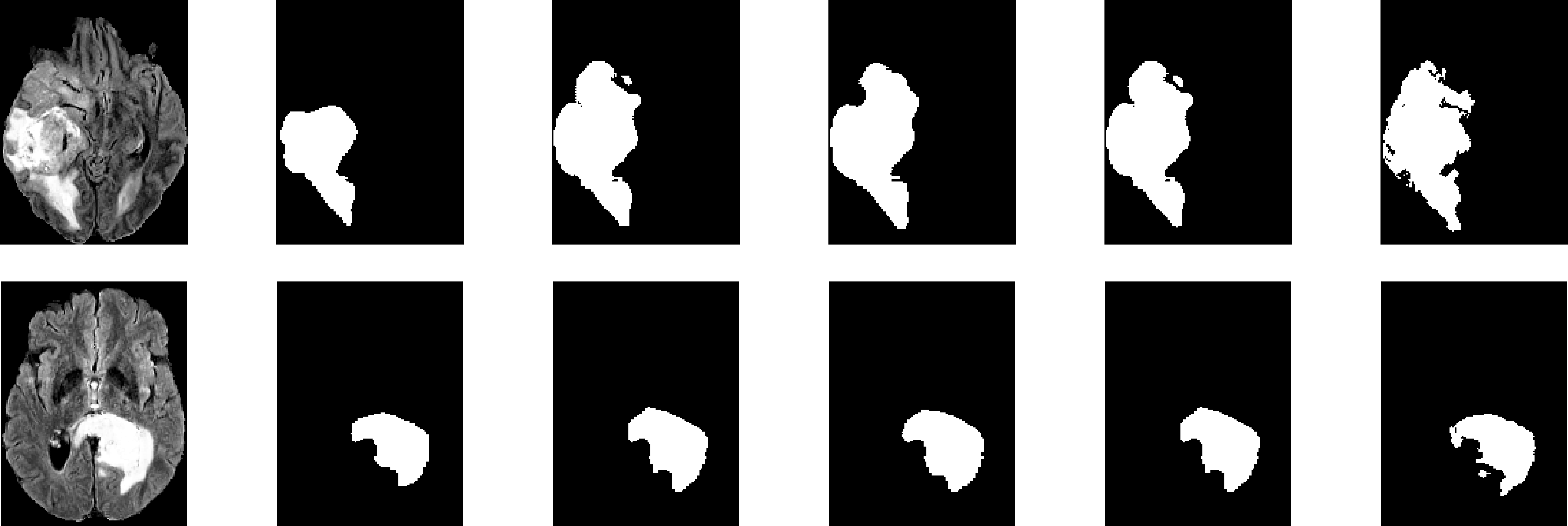
(a) Examples from BraTS dataset.

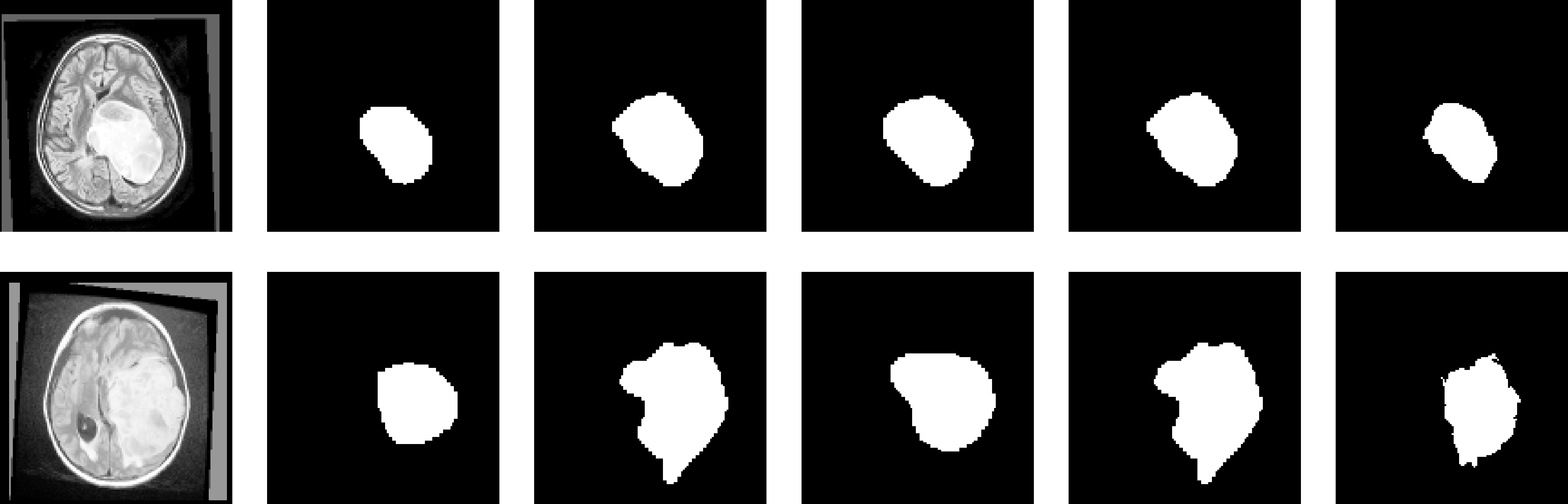
(b) Examples from pLGG dataset.

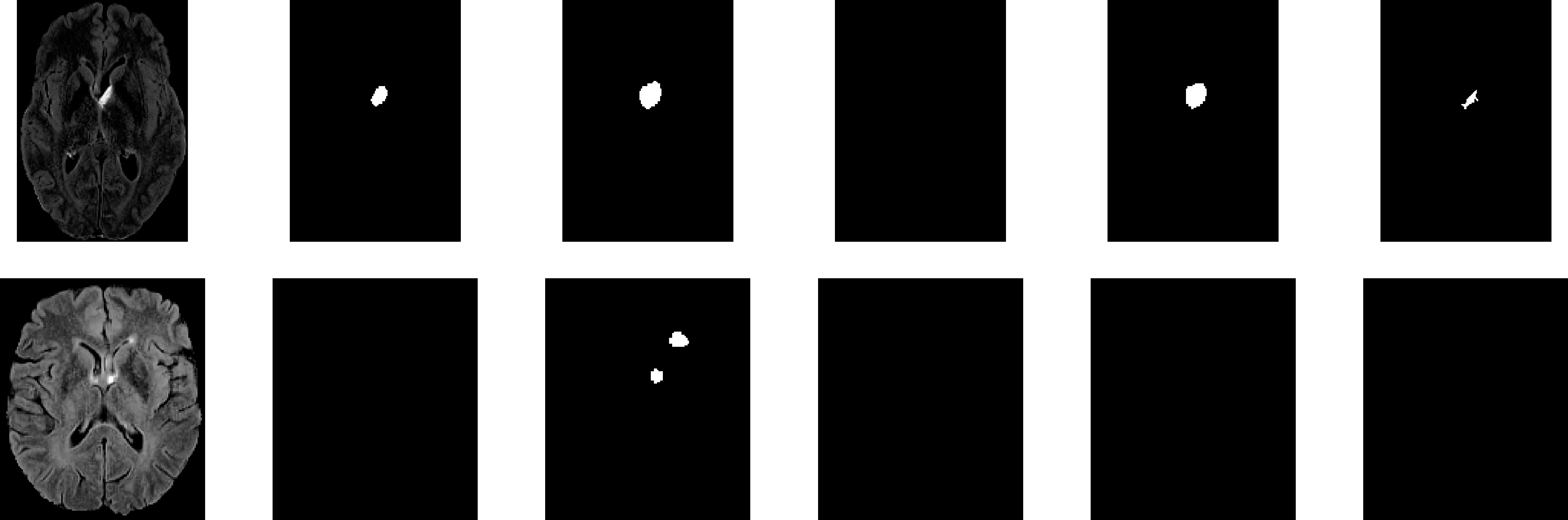
(c) Example from BraTS dataset demonstrating the effectiveness of the combined model.

Fig. 11: From left to right: MR image FLAIR channel, initial model segmentation, oversegmenting model segmentation, undersegmenting model segmentation, combined model segmentation, and true segmentation.

4.4 Comparison to Baselines

We compared the results of our segmentation models to two baseline methods. The first is the initial model trained solely using the seed loss. The second is by taking the L1 distance between the FLAIR channel of an image and its non-cancerous variant, applying a median filter with a 5x5x5 filter, and then thresholding the filtered L1 distance map, as was done by [20] when they acquired their state-of-the-art results for 2D MR weakly supervised glioma segmentation. These results are presented in Table 5.

These results demonstrate that for both datasets, the proposed appproach improves on both baselines. The proposed approach significantly outperformed the baseline methods using the BraTS dataset. These results also show that despite the refined segmentations being negligibly worse than the initial segmentations when using the proposed approach on the pLGG dataset, on which the classifier was unable to acquire a strong understanding of glioma, the refined segmentations still outperformed the baseline segmentation methods.

Table 5: Mean Dice on whole 2D MR images using the initial and combined models compared to baseline methods.

Dataset	Method	Training	Validation	Test
BraTS	Baseline Seed Only	0.5423	0.5218	0.5491
	Baseline L1 Distance	$0.4254$	$0.4295$	$0.4724$
	Proposed Initial	$0.7627$	$0.7659$	$0.7594$
	Proposed Combined	$\mathbf{0.7903}$	$\mathbf{0.7868}$	$\mathbf{0.7712}$
pLGG	Baseline Seed Only	0.6944	0.6910	0.6783
	Baseline L1 Distance	$0.6716$	$0.6772$	$0.6679$
	Proposed Initial	0.7002	0.6955	0.6863
	Proposed Combined	$0.6942$	$0.6911$	$0.6844$

4.5 Difference Score for Filtering Poor Segmentations

We evaluated how the mean Dice changes with different cutoff values when using our proposed weakly supervised filtering method on the segmentations from the combined model. Table 6 presents the mean Dice of the retained segmentations and the percentage of images removed. As was done for the results presented in Tables 4, the results in Table 6 are from 5 separately trained models, whose mean Dice coefficients have been averaged. For brevity, neither the difference score thresholds above 0.3 nor the confidence intervals have been included in Table 6. Difference score thresholds above 0.3 were not included because the Dice coefficients began to stagnate at thresholds above 0.3. Tables with all the difference score thresholds and the mean Dice of removed segmentations, as well as the confidence intervals can be found in Appendices A and B.

Table 6: Mean Dice for kept segmentations and percentage of images removed when applying the proposed difference score-based filtering at different thresholds, averaged across 5 separately trained models.

Dataset	Difference Score Threshold	Mean Dice on Kept Segmentations			Percentage of Images Removed
		Training	Validation	Test	Training	Validation	Test
BraTS	0.0	0.7903	0.7868	0.7712	0.0000	0.0000	0.0000
	0.1	0.8041	0.7904	0.7792	4.6102	0.9075	1.7491
	0.2	0.8235	0.8052	0.7985	14.251	6.6306	7.0464
	0.3	0.8374	0.8232	0.8136	22.735	16.929	14.499
pLGG	0.0	0.6942	0.6911	0.6844	0.0000	0.0000	0.0000
	0.1	0.6968	0.6952	0.6853	0.4566	0.6439	0.1609
	0.2	0.7227	0.7334	0.7055	5.6106	7.7832	4.3467
	0.3	0.7403	0.7362	0.7109	9.9311	8.6811	6.5820

It can be seen that the Dice improves at each threshold interval between 0.1 to 0.3. Choosing the the threshold is a trade off between the mean Dice and the number of segmentations removed, with higher thresholds increasing the mean Dice but removing more segmentations. In most cases, we recommend a threshold of 0.2 as we found it provides a balance between the mean Dice and the number of images removed. For the BraTS dataset, we observed a 2.73% improvement in Dice while only removing 7% of the images for the test cohort when using a threshold of 0.2. This approximate improvement and number of images removed was consistent across all cohorts in this dataset excluding the training cohort for the BraTS dataset, which observed a significantly higher percentage of images removed compared to the rest of the cohorts. In cases where the quality of segmentations is much more valuable than the number of segmentations, such as for semi-supervised methods, we recommend a threshold of 0.3.

Figure 12 presents examples of segmentations that were removed at each threshold from 0.1 to 0.3.

(a) Difference score threshold of 0.1.

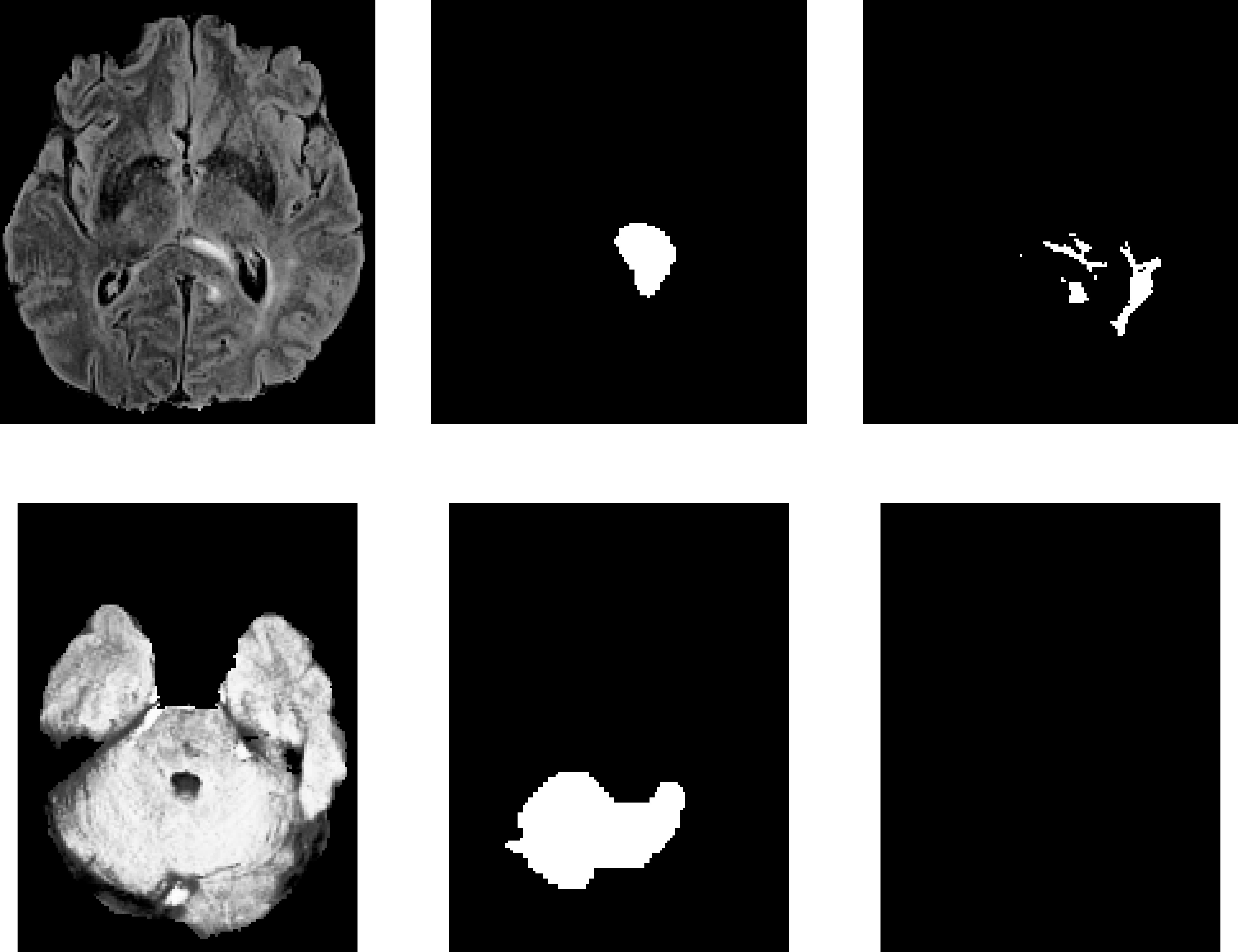
(b) Difference score threshold of 0.2.

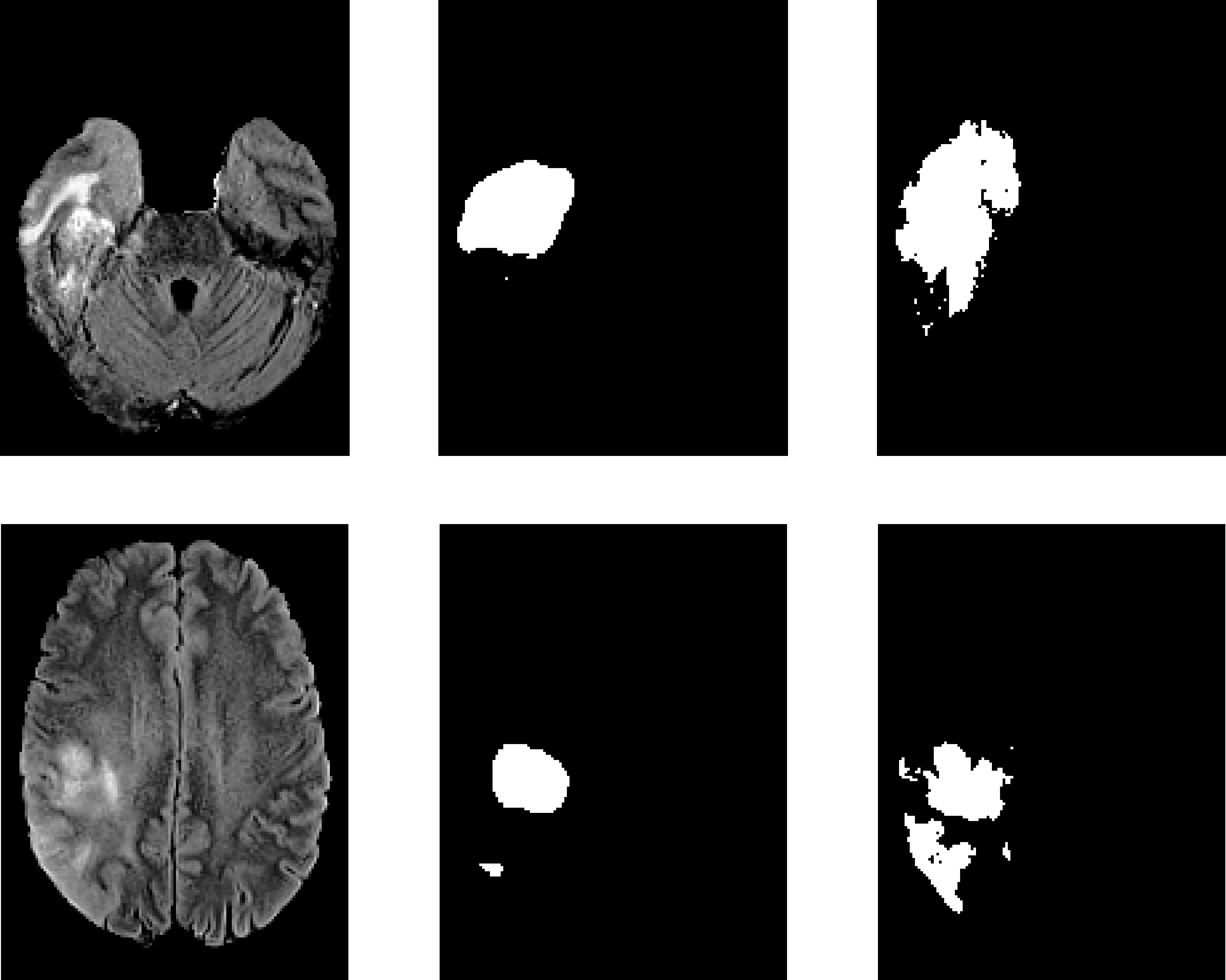
(c) Difference score threshold of 0.3.

Fig. 12: Examples of MR image FLAIR channel removed using the proposed filtering method (left), their corresponding combined model segmentations (middle), and their true segmentations (right) at varying thresholds.

The Pearson correlation coefficient between the difference score and Dice of the segmented MR images for each cohort can be found in Appendix C. These correlations demonstrate a positive correlation between the difference score threshold and the Dice across all cohorts.

5 Discussion

Our proposed method not only enables effective weakly supervised segmentation of brain MR images, but can also be applied to a range of image modalities and anomalies to be segmented, so long as a dataset of images with and without the anomalies is available. The method is also adaptable, as different seed generation methods, classifier model architectures, and segmentation model architectures can be used to improve the performance of the proposed method. Furthermore, this method can be applied to 3D volumes as well, which would enable the model to use the 3D context to potentially improve results.

The proposed filtering method also enables poorer segmentations to be removed, resulting with a large subset of excellent segmentations, whose quality and quantity can increase and decrease at a trade-off based on the threshold selected for the filtering. This allows the filtering to be used to identify a small set of images that may require manual segmentation, or to generate a smaller set of refined segmentations to be used for semi-supervised segmentation, or other tasks that may require a balance of segmentation quality and number of images removed.

Another advantage of the proposed method is that unlike methods that solely use non-cancerous variations from GANs to generate segmentations, our method does not require perfect non-cancerous variants. Baur et al. [20] solely used GAN generated non-cancerous variants and found that the training can lead to generating unrealistic looking images, requiring early stopping to circumvent. Figure 13 demonstrates a flawed non-cancerous variant and a visualizing of its L1 loss compared to the original cancerous image. Despite the flaws in the generated image, the L1 loss map still effectively captures the tumor, making it an effective source of information despite its flaws.

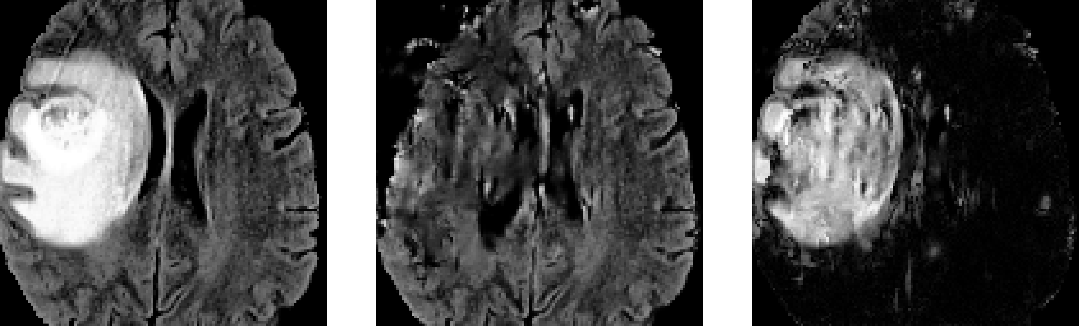
Fig. 13: MR image FLAIR channel (left), its corresponding generated non-cancerous variant (middle), and the L1 distance map between the original image and its non-cancerous variant (right).

While this method produced results exceeding that of the state of the art results for 2D weakly supervised segmentation, the results could be further improved. As noted by Han et al. [19], the ground-truth segmentations from the BraTS dataset, which are based on 3D volumes, can be ”highly incorrect/ambiguous on 2D slices.” While their work was on the 2016 BraTS dataset, we observed such incorrect and ambiguous segmentations in the both the BraTS 2020 dataset and the pLGG as well. While our method does not rely on segmentations, the incorrect/ambiguous segmentations resulted with many images whose segmentations were not removed using the erosion described in Section 3.1 yet had segmented regions that do not have discernible tumors. This resulted with many non-cancerous images being labelled as cancerous, worsening the classifier’s training and thus worsening the overall performance of the method. These incorrect/ambiguous segmentations also negatively affected the Dice coefficient values presented. Figure 14 presents one such example. The ground truth segmentation is negligibly present in the image but despite the segmentation model outputting an empty segmentation as it should, this accurate segmentation scored a Dice of 0.1250. Some ambiguous segmentations also negatively affected the reported performance of the model. Figure 15 presents an example with an ambigiously incorrect ground truth segmentation whose predicted segmentation only achieved a Dice of 0.5040.

Fig. 14: MR image FLAIR channel (left), its corresponding combined model segmentation (middle), and its incorrect/ambiguous true segmentation (right).

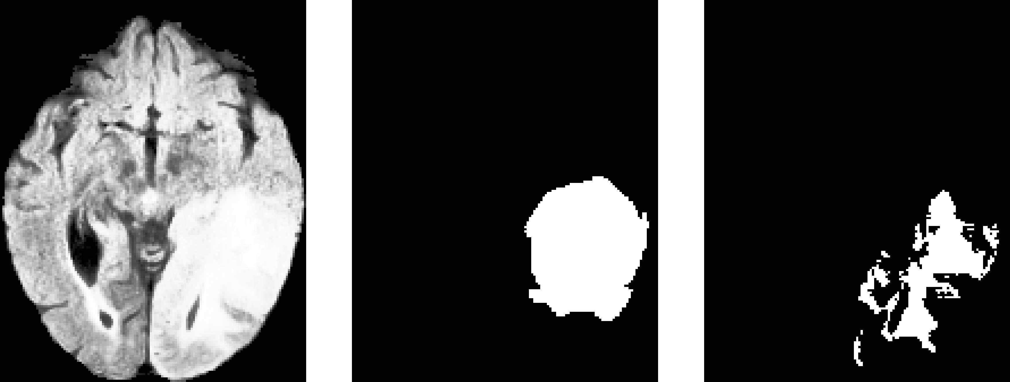
Fig. 15: MR image FLAIR channel (left), its corresponding combined model segmentation (middle), and its incorrect/ambiguous true segmentation (right).

As with all other classifier-based weakly supervised segmentation methods, one notable flaw of the proposed method is its reliance on the initial classifier. Despite steps taken to combat inaccurate biases in the classifier such as the use of non-cancerous images acquired independently of the classifier’s positive seeds, the method is still highly dependent on the classifier. Figure 16 demonstrates this flaw. As patches classified as non-cancerous yield empty segmentations, the presence of segmentations indicates that the classifier classified patches in this non-cancerous image to be cancerous. Upon closer inspection, the classifier when passed the bottom two patches for this image outputted probabilities of 0.8162 and 0.8596. Thus, despite the extremely high performance of the model presented in Table 2, the classifier’s understanding of tumors is still imperfect. The impact of this flaw was exacerbated with the pLGG dataset, as Table 3 indicated that the initial seeds for the pLGG dataset were much worse compared to the initial seeds for the BraTS dataset, indicating that the classifier trained using the pLGG dataset had a significantly worse understanding of glioma. This also impacted the seed and segmentation refinement process as it is highly reliant on the classifier. We observed that the refinement improved the BraTS segmentations but negligibly impacted the pLGG segmentations, as the pLGG trained classifier’s understanding of glioma was not sufficient for the refinement to work for the pLGG dataset. These results indicate that an improved classifier could drastically improve the performance of the method, but at the same time, a flawed classifier could worsen the performance.

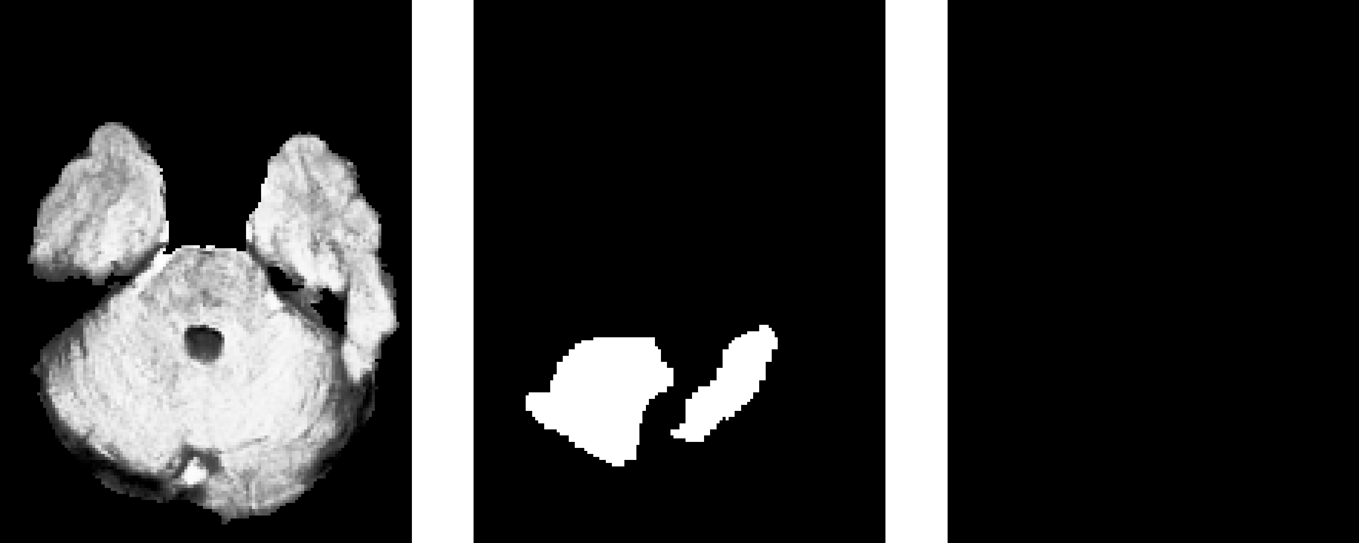
Fig. 16: MR image FLAIR channel classified as false positive (left), its corresponding combined model segmentation (middle), and its true segmentation (right).

6 Conclusion

We present a weakly supervised method for segmenting tumors in 2D MR images that builds on seeded and GAN-based weakly supervised methods and a weakly supervised filtering approach that removes a small subset of poorly segmented images, resulting in a large subset of high-quality segmentations. The novel combination of seeds and GANs surpasses state-of-the-art methods for weakly supervised segmentation on 2D MR images of brains. Furthermore, depending on the threshold used for the filtering approach, the weakly supervised segmentations can be used for semi-supervised segmentation, and can have potential clinical applications as a tool used to reliably segment MR images, leaving a small subset of uncertain images for radiologists to manually investigate and segment, greatly relieving radiologists of the workload that would be required to manually segment all MR images.

Appendices

Appendix A Complete Table of Difference Score Thresholds and Corresponding Mean Dice of Kept Segmentations, Mean Dice of Removed Segmentations, and Percentage of Images Removed

Table 1: Mean Dice for kept and removed segmentations, and percentage of images removed when applying the proposed difference score-based filtering at different thresholds, averaged across 5 models separately trained on the BraTS dataset

Difference Score Threshold	Mean Dice on Kept Segmentations			Mean Dice on Removed Segmentations			Percentage of Images Removed
	Training	Validation	Test	Training	Validation	Test	Training	Validation	Test
0.0	0.7903	0.7868	0.7712	N/A	N/A	N/A	0.0000	0.0000	0.0000
0.1	0.8041	0.7904	0.7792	0.5046	0.3901	0.3217	4.6102	0.9075	1.7491
0.2	0.8235	0.8052	0.7985	0.5904	0.5261	0.4104	14.251	6.6306	7.0464
0.3	0.8374	0.8232	0.8136	0.6300	0.6075	0.5209	22.735	16.929	14.499
0.4	0.8397	0.8256	0.8176	0.6790	0.6820	0.6233	30.749	27.067	23.904
0.5	0.8381	0.8244	0.8137	0.705	0.7167	0.6884	35.916	34.972	33.924
0.6	0.8367	0.8204	0.8105	0.7133	0.7348	0.7034	37.632	39.385	36.716
0.7	0.8366	0.8206	0.8106	0.7137	0.7347	0.7033	37.725	39.393	36.720
0.8	0.8367	0.8207	0.8107	0.7136	0.7345	0.7032	37.731	39.405	36.728
0.9	0.8367	0.8207	0.8107	0.7136	0.7345	0.7032	37.733	39.405	36.728

Table 2: Mean Dice for kept and removed segmentations, and percentage of images removed when applying the proposed difference score-based filtering at different thresholds, averaged across 5 models separately trained on the pLGG dataset

Difference Score Threshold	Mean Dice on Kept Segmentations			Mean Dice on Removed Segmentations			Percentage of Images Removed
	Training	Validation	Test	Training	Validation	Test	Training	Validation	Test
0.0	0.6942	0.6911	6844	N/A	N/A	N/A	0.0000	0.0000	0.0000
0.1	0.6968	0.6952	0.6853	0.1145	0.0394	0.0419	0.4566	0.6439	0.1609
0.2	0.7227	0.7334	0.7055	0.2132	0.1887	0.2171	5.6106	7.7832	4.3467
0.3	0.7403	0.7362	0.7109	0.2752	0.2155	0.3067	9.9311	8.6811	6.5820
0.4	0.7417	0.7362	0.7112	0.2865	0.2155	0.3052	10.448	8.6811	6.6253
0.5	0.7425	0.7362	0.7112	0.2843	0.2155	0.3052	10.560	8.6811	6.6253
0.6	0.7425	0.7362	0.7112	0.2843	0.2155	0.3052	10.560	8.6811	6.6253
0.7	0.7425	0.7362	0.7112	0.2843	0.2155	0.3052	10.560	8.6811	6.6253
0.8	0.7425	0.7362	0.7112	0.2843	0.2155	0.3052	10.560	8.6811	6.6253
0.9	0.7425	0.7362	0.7112	0.2843	0.2155	0.3052	10.560	8.6811	6.6253

Appendix B Confidence Intervals for Table of Difference Score Thresholds and Corresponding Mean Dice of Kept Segmentations, Mean Dice of Removed Segmentations, and Percentage of Images Removed

Table 1: Confidence intervals of mean Dice for kept and removed segmentations, and percentage of images removed when applying the proposed difference score-based filtering at different thresholds across 5 models separately trained on the BraTS dataset

Difference Score Threshold	Mean Dice on Kept Segmentations			Mean Dice on Removed Segmentations			Percentage of Images Removed
	Training	Validation	Test	Training	Validation	Test	Training	Validation	Test
0.0	$4.736610-4$	$7.086410-4$	$1.323510-3$	N/A	N/A	N/A	0.0000	0.0000	0.0000
0.1	$2.002410-04$	$1.028310-03$	$1.656110-03$	$8.653410-03$	$3.389410-02$	$2.182310-02$	$1.137710-01$	$6.149110-02$	$1.312610-01$
0.2	$1.601510-04$	$9.223310-04$	$1.202010-03$	$4.724910-03$	$4.882110-03$	$1.084710-02$	$1.318510-01$	$6.986510-02$	$2.501710-01$
0.3	$2.145810-04$	$9.836310-04$	$1.276710-03$	$3.578010-03$	$3.502610-03$	$8.015810-03$	$1.928010-01$	$1.769910-01$	$2.317310-01$
0.4	$3.853910-04$	$7.713710-04$	$1.672910-03$	$2.482510-03$	$2.346810-03$	$5.495210-03$	$1.496310-01$	$1.599910-01$	$2.903210-01$
0.5	$3.921910-04$	$8.486210-04$	$2.126110-03$	$1.657010-03$	$1.911910-03$	$4.715010-03$	$8.446010-02$	$2.259110-01$	$1.112110-01$
0.6	$4.403610-04$	$8.220510-04$	$1.950810-03$	$1.279810-03$	$1.577110-03$	$3.809210-03$	$5.593210-02$	$8.787910-02$	$1.996510-01$
0.7	$4.296110-04$	$8.955510-04$	$2.008910-03$	$1.254110-03$	$1.630310-03$	$3.851310-03$	$5.447610-02$	$9.477910-02$	$2.044110-01$
0.8	$4.377010-04$	$9.215910-04$	$2.074510-03$	$1.256910-03$	$1.520810-03$	$3.883110-03$	$5.545410-02$	$9.170710-02$	$2.091610-01$
0.9	$4.229110-04$	$9.215910-04$	$2.074510-03$	$1.252510-03$	$1.520810-03$	$3.883110-03$	$5.401610-02$	$9.170710-02$	$2.091610-01$

Table 2: Confidence intervals of mean Dice for kept and removed segmentations, and percentage of images removed when applying the proposed difference score-based filtering at different thresholds across 5 models separately trained on the pLGG dataset

Difference Score Threshold	Mean Dice on Kept Segmentations			Mean Dice on Removed Segmentations			Percentage of Images Removed
	Training	Validation	Test	Training	Validation	Test	Training	Validation	Test
0.0	$5.001710-4$	$2.600210-4$	$4.820210-4$	N/A	N/A	N/A	0.0000	0.0000	0.0000
0.1	$6.208610-04$	$4.456610-04$	$3.732310-04$	$1.027810-02$	$2.495010-02$	$4.873610-03$	$2.696710-02$	$3.988410-02$	$2.030810-02$
0.2	$4.441810-04$	$5.414510-04$	$3.314110-04$	$8.836210-04$	$9.527110-03$	$6.181310-03$	$1.780710-01$	$1.220910-01$	$2.171010-02$
0.3	$2.038710-04$	$2.170910-04$	$5.259710-04$	$4.795110-03$	$2.926110-03$	$7.394510-03$	$4.145710-02$	$2.767510-02$	$7.789910-02$
0.4	$5.894010-05$	$2.170910-04$	$1.295310-04$	$5.056210-03$	$2.926110-03$	$6.346510-03$	$7.243710-03$	$2.767510-02$	$1.716310-02$
0.5	$3.512110-05$	$2.170910-04$	$1.295310-04$	$4.963110-03$	$2.926110-03$	$6.346510-03$	$4.500210-03$	$2.767510-02$	$1.716310-02$
0.6	$3.512110-05$	$2.170910-04$	$1.295310-04$	$4.963110-03$	$2.926110-03$	$6.346510-03$	$4.500210-03$	$2.767510-02$	$1.716310-02$
0.7	$3.512110-05$	$2.170910-04$	$1.295310-04$	$4.963110-03$	$2.926110-03$	$6.346510-03$	$4.500210-03$	$2.767510-02$	$1.716310-02$
0.8	$3.512110-05$	$2.170910-04$	$1.295310-04$	$4.963110-03$	$2.926110-03$	$6.346510-03$	$4.500210-03$	$2.767510-02$	$1.716310-02$
0.9	$3.512110-05$	$2.170910-04$	$1.295310-04$	$4.963110-03$	$2.926110-03$	$6.346510-03$	$4.500210-03$	$2.767510-02$	$1.716310-02$

Appendix C Pearson Correlation Coefficients Between Difference Score Threshold and Dice

The Pearson correlation coefficient between the difference score and Dice of the segmented MR images for each cohort are presented in Table 1. These coefficients indicate an approximate positive relationship between the difference scores and Dice.

Table 1: Pearson correlation coefficients between difference score and Dice at each cohort, averaged across 5 separately trained models

Dataset	Training	Validation	Test
BraTS	$0.4831\pm$9.217310-3$$	$0.4969\pm$5.435010-3$$	$0.6303\pm$8.140710-3$$
pLGG	$0.3615\pm$5.073410-3$$	$0.6225\pm$2.723610-2$$	$0.4348\pm$1.124810-2$$

References

- McDonald et al. [2015] Robert J. McDonald, Kara M. Schwartz, Laurence J. Eckel, et al. The effects of changes in utilization and technological advancements of cross-sectional imaging on radiologist workload. Academic Radiology, 22(9):1191–1198, 2015. ISSN 1076-6332. doi: https://doi.org/10.1016/j.acra.2015.05.007. URL https://www.sciencedirect.com/science/article/pii/S1076633215002457.
- Razzak et al. [2018] Muhammad Imran Razzak, Saeeda Naz, and Ahmad Zaib. Deep Learning for Medical Image Processing: Overview, Challenges and the Future, pages 323–350. Springer International Publishing, Cham, 2018. ISBN 978-3-319-65981-7. doi: 10.1007/978-3-319-65981-7˙12. URL https://doi.org/10.1007/978-3-319-65981-7_12.
- Zhang et al. [2021a] Silu Zhang, Angela Edwards, Shubo Wang, et al. A prior knowledge based tumor and tumoral subregion segmentation tool for pediatric brain tumors. ArXiv, abs/2109.14775, 2021a.
- Liang et al. [2019] Qiaokang Liang, Yang Nan, Gianmarc Coppola, et al. Weakly supervised biomedical image segmentation by reiterative learning. IEEE Journal of Biomedical and Health Informatics, 23(3):1205–1214, May 2019. ISSN 2168-2194, 2168-2208. doi: 10.1109/JBHI.2018.2850040.
- Yang et al. [2020] Guanyu Yang, Chuanxia Wang, Jian Yang, et al. Weakly-supervised convolutional neural networks of renal tumor segmentation in abdominal cta images. BMC Medical Imaging, 20(1):37, Dec 2020. ISSN 1471-2342. doi: 10.1186/s12880-020-00435-w.
- Zhang et al. [2021b] Dong Zhang, Bo Chen, Jaron Chong, and Shuo Li. Weakly-supervised teacher-student network for liver tumor segmentation from non-enhanced images. Medical Image Analysis, 70:102005, May 2021b. ISSN 13618415. doi: 10.1016/j.media.2021.102005.
- Li et al. [2019] Chao Li, Xinggang Wang, Wenyu Liu, et al. Weakly supervised mitosis detection in breast histopathology images using concentric loss. Medical Image Analysis, 53:165–178, Apr 2019. ISSN 13618415. doi: 10.1016/j.media.2019.01.013.
- Ji et al. [2019] Zhanghexuan Ji, Yan Shen, Chunwei Ma, and Mingchen Gao. Scribble-based hierarchical weakly supervised learning for brain tumor segmentation. In Dinggang Shen, Tianming Liu, Terry M. Peters, et al., editors, Medical Image Computing and Computer Assisted Intervention – MICCAI 2019, pages 175–183, Cham, 2019. Springer International Publishing. ISBN 978-3-030-32248-9.
- Feng et al. [2017] Xinyang Feng, Jie Yang, Andrew F. Laine, and Elsa D. Angelini. Discriminative localization in cnns for weakly-supervised segmentation of pulmonary nodules. In Maxime Descoteaux, Lena Maier-Hein, Alfred Franz, et al., editors, Medical Image Computing and Computer Assisted Intervention - MICCAI 2017, pages 568–576, Cham, 2017. Springer International Publishing. ISBN 978-3-319-66179-7.
- Wu et al. [2019] Kai Wu, Bowen Du, Man Luo, et al. Weakly supervised brain lesion segmentation via attentional representation learning. In Dinggang Shen, Tianming Liu, Terry M. Peters, et al., editors, Medical Image Computing and Computer Assisted Intervention – MICCAI 2019, pages 211–219, Cham, 2019. Springer International Publishing. ISBN 978-3-030-32248-9.
- Tang et al. [2020] Yu-Xing Tang, You-Bao Tang, Yifan Peng, et al. Automated abnormality classification of chest radiographs using deep convolutional neural networks. npj Digital Medicine, 3(1):1–8, 2020.
- Zhou et al. [2016] Bolei Zhou, Aditya Khosla, Agata Lapedriza, et al. Learning deep features for discriminative localization. In 2016 IEEE Conference on Computer Vision and Pattern Recognition (CVPR), pages 2921–2929, 2016. doi: 10.1109/CVPR.2016.319.
- Patel and Dolz [2022] Gaurav Patel and Jose Dolz. Weakly supervised segmentation with cross-modality equivariant constraints. Medical Image Analysis, 77:102374, 2022. ISSN 1361-8415. doi: https://doi.org/10.1016/j.media.2022.102374. URL https://www.sciencedirect.com/science/article/pii/S1361841522000275.
- Lerousseau et al. [2021] Marvin Lerousseau, Maria Vakalopoulou, Marion Classe, et al. Weakly supervised multiple instance learning histopathological tumor segmentation, 2021.
- Ribeiro et al. [2016] Marco Tulio Ribeiro, Sameer Singh, and Carlos Guestrin. ”Why Should I Trust You?”: Explaining the predictions of any classifier. In Proceedings of the 22nd ACM SIGKDD International Conference on Knowledge Discovery and Data Mining, KDD ’16, page 1135–1144, New York, NY, USA, 2016. Association for Computing Machinery. ISBN 9781450342322. doi: 10.1145/2939672.2939778. URL https://doi.org/10.1145/2939672.2939778.
- Lundberg et al. [2020] Scott M. Lundberg, Gabriel Erion, Hugh Chen, et al. From local explanations to global understanding with explainable ai for trees. Nature Machine Intelligence, 2(1):56–67, Jan 2020. ISSN 2522-5839. doi: 10.1038/s42256-019-0138-9.
- Petsiuk et al. [2018] Vitali Petsiuk, Abir Das, and Kate Saenko. Rise: Randomized input sampling for explanation of black-box models. In BMVC, 2018.
- Goodfellow et al. [2020] Ian Goodfellow, Jean Pouget-Abadie, Mehdi Mirza, et al. Generative adversarial networks. Commun. ACM, 63(11):139–144, oct 2020. ISSN 0001-0782. doi: 10.1145/3422622. URL https://doi.org/10.1145/3422622.
- Han et al. [2019] Changhee Han, Leonardo Rundo, Ryosuke Araki, et al. Combining noise-to-image and image-to-image gans: Brain mr image augmentation for tumor detection. IEEE Access, 7:156966–156977, 2019. doi: 10.1109/ACCESS.2019.2947606.
- Baur et al. [2019] Christoph Baur, Benedikt Wiestler, Shadi Albarqouni, and Nassir Navab. Deep autoencoding models for unsupervised anomaly segmentation in brain mr images. In Alessandro Crimi, Spyridon Bakas, Hugo Kuijf, et al., editors, Brainlesion: Glioma, Multiple Sclerosis, Stroke and Traumatic Brain Injuries, pages 161–169, Cham, 2019. Springer International Publishing. ISBN 978-3-030-11723-8.
- Baur et al. [2021] Christoph Baur, Benedikt Wiestler, Mark Muehlau, et al. Modeling healthy anatomy with artificial intelligence for unsupervised anomaly detection in brain mri. Radiology: Artificial Intelligence, 3(3):e190169, May 2021. ISSN 2638-6100. doi: 10.1148/ryai.2021190169. URL http://pubs.rsna.org/doi/10.1148/ryai.2021190169.
- Ronneberger et al. [2015] Olaf Ronneberger, Philipp Fischer, and Thomas Brox. U-net: Convolutional networks for biomedical image segmentation. In Nassir Navab, Joachim Hornegger, William M. Wells, and Alejandro F. Frangi, editors, Medical Image Computing and Computer-Assisted Intervention – MICCAI 2015, pages 234–241, Cham, 2015. Springer International Publishing. ISBN 978-3-319-24574-4.
- Szegedy et al. [2016] Christian Szegedy, Vincent Vanhoucke, Sergey Ioffe, et al. Rethinking the inception architecture for computer vision. In 2016 IEEE Conference on Computer Vision and Pattern Recognition (CVPR), pages 2818–2826, 2016. doi: 10.1109/CVPR.2016.308.
- Kullback and Leibler [1951] S. Kullback and R. A. Leibler. On Information and Sufficiency. The Annals of Mathematical Statistics, 22(1):79 – 86, 1951. doi: 10.1214/aoms/1177729694. URL https://doi.org/10.1214/aoms/1177729694.
- Menze et al. [2015] Bjoern H. Menze, Andras Jakab, Stefan Bauer, et al. The multimodal brain tumor image segmentation benchmark (brats). IEEE Transactions on Medical Imaging, 34(10):1993–2024, 2015. doi: 10.1109/TMI.2014.2377694.
- Bakas et al. [2017a] Spyridon Bakas, Hamed Akbari, Aristeidis Sotiras, et al. Advancing The Cancer Genome Atlas glioma MRI collections with expert segmentation labels and radiomic features. Scientific Data, 4(1):170117, December 2017a. ISSN 2052-4463. doi: 10.1038/sdata.2017.117. URL http://www.nature.com/articles/sdata2017117.
- Bakas et al. [2019] Spyridon Bakas, Mauricio Reyes, Andras Jakab, et al. Identifying the best machine learning algorithms for brain tumor segmentation, progression assessment, and overall survival prediction in the brats challenge. Apr 2019. doi: 10.17863/CAM.38755. URL https://www.repository.cam.ac.uk/handle/1810/291597.
- Bakas et al. [2017b] Spyridon Bakas, Hamed Akbari, Aristeidis Sotiras, et al. Segmentation Labels for the Pre-operative Scans of the TCGA-LGG collection, 2017b. URL https://wiki.cancerimagingarchive.net/x/LIZyAQ. Type: dataset.
- Bakas et al. [2017c] Spyridon Bakas, Hamed Akbari, Aristeidis Sotiras, et al. Segmentation Labels for the Pre-operative Scans of the TCGA-GBM collection, 2017c. URL https://wiki.cancerimagingarchive.net/x/KoZyAQ. Type: dataset.
- Henry et al. [2021] Théophraste Henry, Alexandre Carré, Marvin Lerousseau, et al. Brain tumor segmentation with self-ensembled, deeply-supervised 3d u-net neural networks: A brats 2020 challenge solution. In Alessandro Crimi and Spyridon Bakas, editors, Brainlesion: Glioma, Multiple Sclerosis, Stroke and Traumatic Brain Injuries, pages 327–339, Cham, 2021. Springer International Publishing. ISBN 978-3-030-72084-1.
- Paszke et al. [2019] Adam Paszke, Sam Gross, Francisco Massa, et al. Pytorch: An imperative style, high-performance deep learning library. In H. Wallach, H. Larochelle, A. Beygelzimer, et al., editors, Advances in Neural Information Processing Systems 32, pages 8024–8035. Curran Associates, Inc., 2019. URL http://papers.neurips.cc/paper/9015-pytorch-an-imperative-style-high-performance-deep-learning-library.pdf.