Unified fluid-model theory of $\mathbf{E}\times\mathbf{B}$ instabilities in low-ionized collisional plasmas with arbitrarily magnetized multi-species ions

Abstract

This paper develops a unified linear theory of local cross-field plasma instabilities, such as the Farley-Buneman, electron thermal, and ion thermal instabilities, in collisional plasmas with fully or partially unmagnetized multi-species ions. Collisional plasma instabilities in low-ionized, highly dissipative, weakly magnetized plasmas play an important role in the lower Earth’s ionosphere and may be of importance in other planet ionospheres, star atmospheres, cometary tails, molecular clouds, accretion disks, etc. In the solar chromosphere, macroscopic effects of collisional plasma instabilities may contribute into significant heating — an effect originally suggested from spectroscopic observations and relevant modeling. Based on a simplified 5-moment multi-fluid model, the theoretical analysis produces the general linear dispersion relation for the combined Thermal-Farley-Buneman Instability (TFBI). Important limiting cases are analyzed in detail. The analysis demonstrates acceptable applicability of this model for the processes under study. Fluid-model simulations usually require much less computer resources than do more accurate kinetic simulations, so that the apparent success of this approach to the linear theory of collisional plasma instabilities makes it possible to investigate the TFBI (along with its possible macroscopic effects) using global fluid codes originally developed for large-scale modeling of the solar and planetary atmospheres.

I INTRODUCTION

This paper develops a unified linear theory of local cross-field plasma instabilities, such as the Farley-Buneman instability (FBI) [1, 2], electron thermal instability (ETI) [3, 4, 5, 6], and ion thermal instability (ITI) [7, 8]. These instabilities may occur in low-ionized and highly dissipative plasmas embedded in crossed electric and magnetic fields. Such conditions are typical for the lower (E-region) Earth’s ionosphere, solar chromosphere, other planetary ionospheres, and they could exist in such low-ionized gaseous objects as cometary tails, molecular clouds, accretion disks, etc. The above local instabilities, along with the nonlocal gradient drift instability (GDI) [9, 10, 11], generate waves of acoustic-like plasma density perturbations coupled with turbulent electrostatic fields.

All these instabilities have been mostly studied with respect to the E-region ionosphere, but the emphasis of this paper is on the solar chromosphere. The chromosphere is a relatively cool interface between the warmer photosphere and very hot corona. Any energy transferred from the surface of the Sun to the corona necessarily goes though the chromosphere. Therefore, it is crucial to understand this region and properly model its behavior. The solar chromosphere is a highly complex and dynamic region where microphysics may play a significant role. Recently, large improvements in observations and modeling have been made. Radiative MHD models capture a large variety of chromospheric dynamics, such as magneto-acoustic shocks [12, 13], spicules [14, 15], and flux emergence or local dynamos [16].

However, when comparing chromospheric observable profiles, such as MgII from IRIS observations [17] and CaII from ground-based observatories, with synthesis from the above models, the synthetic profiles typically turn out to be narrower than the profiles deduced from observations [18]. This discrepancy could have come from the lack of turbulence in models, but the additional OI lines indicate that this is insufficient [19]. Another possible scenario to explain the discrepancy is mass load or heating. Comparison between IRIS and ALMA observations with radiative MHD single-fluid models, which included ion-neutral interaction effects and non-equilibrium ionization, suggests that spicules in the models are still up to a few thousand degrees lower [20].

Fontenla et al. [21, 22] proposed a new heating mechanism that has not been included in the previous models. This heating mechanism involves plasma turbulence and is based on the analogy between the solar chromosphere and the lower Earth’s ionosphere. In the latter, collisional cross-field instabilities leading to palpable plasma turbulence have been studied extensively using radar and rocket observations, analytic theory, and supercomputer simulations. These instability-driven turbulence produces an important macroscopic effect of strong anomalous electron heating detected by radars [23, 24]. This effect has been explained using analytic models and kinetic simulations [25, 26, 27]. Fontenla et al. [21, 22] suggested that the chromosphere may include similar heating processes. These and other analyses [28, 29, 30, 31, 32] suggested that the collisional cross-field plasma instabilities can really be developed under the chromosphere conditions, so that the proposed heating mechanism is plausible. The accurate theory of the relevant plasma instabilities should help explain how, and by how much, this mechanism could contribute to the chromospheric heating. The linear theory of these instabilities, developed in this paper, is a necessary step in that direction.

In a number of important aspects, the physical conditions of the solar chromosphere are similar to those of the E-region ionosphere. Among the common features are the low ionization and prevalence of plasma-neutral collisions in such a way that electrons are still magnetized, while ions are partially or fully unmagnetized due to their frequent collisions with neutral particles (by magnetized $s$-species plasma particles we mean particles whose gyrofrequency $\Omega_{s}$ is much larger than the ion-neutral mean collision frequency $\nu_{sn}$, while by unmagnetized or partially unmagnetized $s$-species we mean the opposite case of $\Omega_{s}\lesssim\nu_{sn}$). The energy source for the instabilities is the DC electric field $\vec{E}_{0}$ perpendicular to the magnetic field $\vec{B}_{0}$, in the frame of reference attached to the neutral-particle flow. If $\vec{E}_{0}$ is strong enough then the above magnetization conditions lead to cross-field instabilities. In the Earth’s ionosphere, strong electric fields are either generated by a neutral-atmosphere dynamo (in the equatorial E region) or are mapped from the magnetosphere down to the high-latitude E region during geomagnetic storms and other intense events. In the core of the solar chromosphere, where the ideal MHD conditions do not apply, high-speed neutral flows decoupled from the magnetic field and crossing the latter under a significant angle may exist [33, 34, 35, 36]. This translates to the occurrence of strong electric fields in the neutral-flow frame of reference.

On the other hand, the E-region ionosphere and solar chromosphere have noticeable distinctions, such as the differences in the ion and neutral compositions. In the E-region ionosphere, the two major ion species have fairly close molecular masses and collision characteristics, so that to a reasonable accuracy they can be treated as one unified ion species. A totally different situation takes place in the solar chromosphere. The ion composition there may be quite diverse. While the neutral part is mostly H (for simplicity, we ignore here a small contribution of neutral He [37, 38]), the dominant ions are not necessarily protons, H⁺. The ion composition is often dominated by ionized metal and other heavy impurities (C⁺, Mg⁺, Si⁺, Fe⁺, etc.) because the ionization potentials of the corresponding neutral atoms are usually significantly lower than that of H. As a result, the magnetization of various ions may differ dramatically. At a given location, some ion species can be magnetized, while other species are fully or partially unmagnetized [31, 32]. The multi-species ion composition with different magnetization characteristics modifies the conditions of the plasma instability development and complicates their analysis.

Additionally, unlike the lower Earth’s ionosphere where the dominant ions (O${}_{2}^{+}$, NO⁺) and neutrals (N₂, O₂) are molecules, the solar chromosphere consists mostly of atoms. In the E-region ionosphere, within the characteristic range of the characteristic low energies $\lesssim 0.3~{}$eV, electron collisions with neutral molecules, due to the excitation of rotational and vibrational molecular levels, lead to mostly inelastic energy losses. In the solar chromosphere, the electron collisional energy losses are supposed to be mostly elastic since, within the relevant energy range of $\lesssim 1$ eV, the excitation of the atomic electron levels is almost negligible. Using the same arguments, we can safely presume that the contribution of the non-equilibrium ionization [39, 40, 41] is also relatively small. This has serious implications for the electron temperature balance and instability generation, as we discuss in Sec. III.

Finally, the chromospheric magnetic fields are much larger than the geomagnetic field, as well as the chromospheric values of the plasma and neutral temperatures are significantly higher than those in the Earth’s ionosphere. However, these and similar parameters are scalable, so that this quantitative distinction is not a real problem for the theory.

To simulate the above instabilities in both the initial (linear) and later (nonlinear) stages, one can use fluid-model, kinetic, or hybrid approaches. Most accurate is the kinetic approach, especially that based on particle-in-cell (PIC) codes [42, 43, 44, 27, 32]. Such codes usually include all relevant physics, but they typically require substantial computer resources. At present time, the PIC codes can simulate only restricted local plasma volumes during a limited time duration, and those scales are still orders of magnitude smaller than the chromospheric features observed with the current resolution. At the same time, simulations based on simplified fluid-model equations are usually much less restrictive and can efficiently model even global plasma environments, such as, e.g., supergranular scales of the lower solar atmosphere and even entire planetary ionospheres.

Typical wave periods and wavelengths of turbulence generated as a result of collisional plasma instabilities are usually larger than the inverse collision frequencies and mean free paths, respectively. Plasma processes with such temporal and spatial scaling are usually reasonably well described by fluid-model equations, though particle kinetics can sometimes be of paramount importance. Indeed, the growth rate $\gamma$ of the pure FBI increases with the wavenumber $k$ as $\gamma\propto k^{2}$ until the wavelength becomes comparable to the inverse ion-neutral collisional mean free path. For shorter wavelengths (i.e., larger $k$), the kinetic effect of ion Landau damping overcomes the $k^{2}$ increase of $\gamma$ and sharply turns it down to negative values, thus providing total stabilization of the short-wavelength waves, see, e.g., Ref. 45. As a result of this competition, the maximum instability growth rate is typically reached at an intermediate spectral range between the highly and weakly collisional bands which are determined by the low and high ratios of the wavelength to the collisional mean free path, respectively.

The theoretical approach of this paper is based on a simplified 5-moment multi-fluid set of equations. This model includes automatically all relevant mechanisms of the instability driving and dissipation, except the Landau damping and a number of other, mostly inconsequential, factors. For the ionospheric conditions, in the framework of the two-fluid model (electrons and single-species ions) such fluid-model analysis has been performed recently in a series of papers by Makarevich, see Ref. 46 and references therein. Makarevich studied the linear theory of the FBI, GDI, and ITI (but not the ETI) for arbitrary wavelengths, regardless of the fact that the short-wavelength band is beyond the applicability of the fluid model.

In this paper, bearing in mind mostly the conditions of the solar chromosphere, we analyze the general case of multi-species ions with an arbitrary degree of the ion-species magnetization. Furthermore, in the E-region research it is usually implied that the FBI is the dominant and the most energetically efficient instability, solely responsible for the anomalous electron heating. The main reason why we also included in our present theory the thermal instabilities is as follows. Our recent PIC simulations of plasma instabilities under the chromospheric conditions revealed, to our surprise, that the ETI is very important and can even dominate in some regions of the solar chromosphere [32]. As far as the ITI is concerned, our previous research has demonstrated that the ion thermal driving usually accompanies the FBI [8, 43] and hence needs to also be included for consistency.

Our theoretical analysis produces the general linear fluid-model dispersion relation for the combined Thermal-Farley-Buneman Instability (TFBI) that includes all relevant driving mechanisms (except the nonlocal GDI). Our major thrust is on the long-wavelength limit in which all collisional plasma instabilities reach their minimum threshold. This limit is of special importance because if at a given location the driving electric field is below the minimum threshold value then this location is linearly stable for any waves. Although the fluid model is rigorously valid only in the long-wavelength limit, in some cases it is possible, following Makarevich [46], to extend the fluid-model treatment to all wavelengths. In Appendix A, we demonstrate that in spite of the total absence of Landau damping the simplified 5-moment model provides stabilization of sufficiently short-wavelength waves (though the fluid-model results may be inaccurate there). This fact allows one to safely use fully fluid-model equations to simulate all instabilities without fearing that the corresponding code might “explode” within the short-wavelength band because of the absence of Landau damping.

This analytical theory provides predictions of the instability generation threshold conditions and growth rates, depending on the specific local parameters of the plasma media. Also, we demonstrate that the fluid-model approach for simulating the TFBI is reasonably well justified, even without including the important kinetic effect of Landau damping. This guarantees that the global fluid codes developed for the large-scale modeling can be applied to the simulation of the small-scale cross-field plasma instabilities as well. The results of this analytic theory can serve as a guide for such simulations and help analyze their results.

This paper is organized as follows. In Sec. II, we introduce the initial equations. In Sec. III, we describe the background plasma affected by the given imposed electric field in the neutral frame of reference. More specifically, we describe the mean particle flows (Sec. III.1) and ohmic heating (Sec. III.2). The knowledge of the accurate values of these background parameters is crucial for the instability linear theory. In Sec. IV, we consider this linear theory and derive the general multi-fluid dispersion relation for the TFBI. In Sec. V, which is central to this paper, we study the most important limit of long-wavelength waves, which is responsible for the minimum instability threshold. In this limit, to the zeroth-order approximation, we derive the wave phase-velocity relation, which is common for all instabilities (Sec. V.1). To the first-order approximation, in Sec. V.2, we derive the instability driving/damping rates, where separate terms describe the driving mechanisms for each distinct collisional instability and for the total losses. Section V.3 discusses the most important quantitative result of the linear theory of instabilities, i.e., the instability threshold. Section VI discusses the general dispersion relation for arbitrary wanelengths. Section VII summarizes the paper results. Appendix A discusses the short-wavelength limit of the general dispersion relation. The analysis of the short-wavelength limit guarantees that the employed fluid model, even without Landau damping, can be safely used for instabillity modeling at all wavelengths with no need for additional damping mechanisms to stabilize the wave behavior at short wavelengths. Appendix B lists major notations used in the paper.

II INITIAL EQUATIONS

In low-ionized plasmas, the dominant neutral component is usually weakly disturbed by the plasma turbulence, so that within small and short-duration characteristic spatiotemporal scales of instabilities we assume the neutral atmosphere to be spatially uniform and stationary. For simplicity, we will consider the constant neutral background composed of a single-species gas.

The simplest, 5-moment, multi-fluid model includes the continuity, momentum, and energy-balance equations. In the frame of reference moving with the local neutral flow (assumed to be spatially uniform and stationary, as stated above), for each plasma species fluid marked by the subscript $s$, these equations can be written as

$$\frac{\partial n_{s}}{\partial t}+\nabla\cdot(n_{s}\vec{V}_{s})=0,$$ (1a)

$$m_{s}\frac{D_{s}\vec{V}_{s}}{Dt}=q_{s}(\vec{E}+\vec{V}_{s}\times\vec{B})-\frac{\nabla(n_{s}T_{s})}{n_{s}}-m_{s}\nu_{sn}\vec{V}_{s},$$ (1b)

$$n_{s}^{2/3}\ \frac{D_{s}}{Dt}\left(\frac{T_{s}}{n_{s}^{2/3}}\right)=\frac{2}{3}\ M_{sn}\nu_{sn}\vec{V}_{s}^{2}-\delta_{sn}\nu_{sn}(T_{s}-T_{n}),$$ (1c)

where $$D_{s}/Dt=\partial/\partial t+\vec{V}_{s}\cdot\nabla s n_{s} m_{s} q_{s} T_{s} \vec{V}_{s} s \nu_{sn}\ s n M_{sn}=m_{s}m_{n}/(m_{s}+m_{n}) \delta_{sn} \delta_{sn} \delta_{sn}=2m_{s}/(m_{s}+m_{n}) \delta_{en} \delta_{en}\ll 1 \delta_{sn} \vec{E} \vec{B} \vec{B}(\vec{r},t) \vec{B}\approx\vec{B}_{0} q_{e}=-e e q_{i}=e q_{j} j q_{j}/e \geq 1$$ is the substantial derivative along the -flow; , , , , and are the -species particle number density, mass, electric charge, temperature (in energy units), and mean fluid velocity, respectively; is the mean momentum transfer frequency of an -particle collision with a neutral () particle, is the corresponding effective mass, and is the mean collisional energy-loss fraction (the notation should not be confused with the Kronecker delta function). For purely elastic collisions, we have . In the lower Earth’s ionosphere, however, the energy losses are dominated by inelastic electron-neutral (e-n) collisions determined mostly by low-energy molecular rotational and vibrational excitations, so that can be electron-velocity dependent and significantly larger than the elastic value (though still ). In the solar chromosphere, we presume to be close to its elastic value. Further, and are the total electrostatic field and an imposed external magnetic field respectively (both in the neutral-gas frame of reference). Implying sufficiently small-scale and short-period wave perturbations, we assume the large-scale local background magnetic field to be spatially uniform, stationary, and sufficiently strong, so that its wave perturbations caused by turbulent electric currents and non-electrostatic electric fields can be neglected, . For electrons, the particle charge is , where is the elementary charge. In the lower ionosphere, the ions are singly charged, . For the solar chromosphere, however, we cannot exclude the possibility of multiply charged ions, so that we will keep the general average charge for each ion species . Within a given ion species there may be the whole spectrum of discrete particle charges, so that, in principle, the average charge ratio may have a non-integer value .

The simplified fluid-model set of Eq. (1) implies that the $s$-particle velocity distribution, along with its wave perturbations, are reasonably close to Maxwellian. This set of equations includes all essential factors crucial for the instability generation and damping, such as the particle inertia in the left-hand side (LHS) of Eq. (1b), Lorentz force, pressure gradients, and collisional friction ($-m_{s}\nu_{sn}\vec{V}_{s}$) in the right-hand side (RHS) of Eq. (1b), the heat advection and adiabatic heating/cooling in the LHS of Eq. (1c), as well as even more important local collisional heating and cooling in the RHS of Eq. (1c). The somewhat unconventional form of energy-balance Eq. (1c) with its LHS proportional to the substantial derivative of the specific enthropy ($T_{s}/n_{s}^{2/3}$) is more convenient for our purposes. In particular, this form explicitly shows that in the absence of the collisional heating and cooling – the first and second terms of the right-hand side (RHS) respectively – the particle temperature obeys the adiabatic temperature regime, $T_{s}\propto n_{s}^{2/3}$.

Equation (1) neglects a number of known factors that are largely inconsequential for the processes under study, largely due to the aforementioned constraints on the typical turbulence spatial and temporal scales. Among the major neglected factors are: Coulomb collisions between the charged particles, slow processes of ionization and plasma annihilation (recombination), pressure anisotropy (viscosity), higher moments of the particle velocity distributions, the gravity force, and heat conductivity.

In the equatorial and high-latitude E-region ionospheres, the electrojet instabilities are driven by an imposed significant DC electric field $\vec{E}_{0}$. Its scales of spatial and temporal variation are usually much larger than the characteristic wave scales, so that one may treat $\vec{E}_{0}$ as spatially uniform and constant. In the solar chromosphere, neutral flows that originate from below the chromosphere may decouple from the magnetic field and cross the magnetic field lines. In a local frame of the neutral flow moving with the neutral mass velocity $\vec{V}_{n}$ across a given magnetic field, $\vec{B}_{0}$, we have an external large-scale DC electric field $\vec{E}_{0}=-\vec{V}_{n}\times\vec{B}_{0}$. Then the total electrostatic field is $\vec{E}=\vec{E}_{0}-\nabla\Phi$, where $\Phi$ is the electrostatic potential produced by plasma turbulence. Poisson’s equation for $\Phi(r,t)$,

$$\nabla^{2}\Phi=\frac{1}{\epsilon_{0}}\left(en_{e}-\sum_{j=1}^{p}q_{j}n_{j}\right),$$ (2)

closes the electrostatic description of plasma dynamics (here the integer $p$ is the total number of the ion species; $\epsilon_{0}$ is the permittivity of free space). Typical turbulent wavelengths are much larger than the Debye lengths. This usually allows one to employ the quasi-neutrality relation, $en_{e}=\sum_{j=1}^{p}q_{j}n_{j}$, which eliminates the need for Poisson’s equation and simplifies the treatment. Bearing in mind, however, that even small deviations from the quasi-neutrality in plasma waves may sometimes be of importance (as we discuss below), for the linear waves generated by the instabilities we will use Eq. (2). For the large-scale background plasma density $n_{s}=n_{s0}$, we will assume the full local charge neutrality,

$$en_{e0}=\sum_{j=1}^{p}q_{j}n_{j0}.$$ (3)

III BACKGROUND FLOWS AND MEAN OHMIC HEATING

The driving force of all collisional plasma instabilities is the external DC electric field, $\vec{E}_{0}\perp\vec{B}_{0}$, that must exist in the frame of reference attached to the neutral atmosphere. The collisional plasma response to this driving field is twofold: the external field creates distinct electron and ion particle flows (leading to an anisotropic electric current) and it also heats the plasma through the friction caused by collisions of the plasma with the neutral particles. On the one hand, the stronger is the field $\vec{E}_{0}$ the faster are the particle flows and the better should be the conditions for the instability excitation. On the other hand, a stronger field $\vec{E}_{0}$ results in larger mean ohmic heating of the plasma. The elevated electron and ion temperatures increase the plasma diffusion within the waves and, through the increased instability threshold, make the heated plasma more resistive to the instability excitation. If, nonetheless, the driving field magnitude, $E_{0}=|\vec{E}_{0}|$, exceeds the increased instability threshold, $E_{\mathrm{Thr}}$, then the linear instability will develop, but saturated plasma turbulence will be less intense than it might be without such macroscopic heating. In the non-linear stage, the turbulent electric field additionally heats up plasma particles, affecting the saturated level of developed turbulence. In this paper, however, we deal only with the initial linear stage of instabilities.

III.1 Mean particle flows

Consider the undisturbed background plasma embedded in the external macroscopic electric ($\vec{E}_{0}$) and magnetic ($\vec{B}_{0}$) fields. For a given plasma species $s$ (electrons or $j$-species ions), Eq. (1b) yields the following mean fluid velocity:

$$\vec{V}_{s0}=\left.\!\!\left(\frac{q_{s}\vec{E}_{0}}{m_{s}\nu_{sn}}+\kappa_{s}^{2}\vec{V}_{0}\right)\!\!\right/\!\!\!\left(1+\kappa_{s}^{2}\right)=\frac{\kappa_{s}(\vec{E}_{0}+\kappa_{s}\vec{E}_{0}\times\hat{b})}{(1+\kappa_{s}^{2})B_{0}}.$$ (4)

Here

$$\vec{V}_{0}\equiv\frac{\vec{E}_{0}\times\vec{B}_{0}}{B_{0}^{2}}=\frac{\vec{E}_{0}\times\hat{b}}{B_{0}}$$ (5)

is the $\vec{E}_{0}\times\vec{B}_{0}$ drift velocity, where $\hat{b}\equiv\vec{B}_{0}/B_{0}$ is the unit vector in the direction of $\vec{B}_{0}$, $\Omega_{s}=q_{s}B_{0}/m_{s}$ is the $s$-species gyrofrequency, and

$$\kappa_{s}=\frac{\Omega_{s}}{\nu_{sn}}=\frac{q_{s}B_{0}}{m_{s}\nu_{sn}}$$ (6)

is the corresponding magnetization parameter. In this paper, we mostly imply strongly magnetized electrons, $\kappa_{e}^{2}\gg 1$, while a multi-species positive-ion population, $s=j$, may contain both unmagnetized or magnetized ions. In other words, we allow the ion magnetization to be weak, $\kappa_{j}\ll 1$, or moderate, $\kappa_{j}\gtrsim 1$, but not strong (not $\kappa_{j}\gg 1$). Strongly magnetized ions are of no interest for the collisional instabilities, since for $\kappa_{j}>1$ the FBI mechanism becomes stabilizing with the stabilization facor increasing proportionally with $(\kappa_{j}^{2}-1)$, see Ref. 8.

For each ion species $j$, we introduce the difference between the undisturbed electron and ion drift velocities, $\vec{U}_{j}\equiv\vec{V}_{e0}-\vec{V}_{j0}$. We will actively use this parameter in the following sections. Strongly magnetized electrons move with almost the $\vec{E}_{0}\times\vec{B}_{0}$ drift velocity, $\vec{V}_{e0}\approx\vec{V}_{0}$, so that Eq. (4) yields

$$\vec{U}_{j}\approx\vec{V}_{0}-\vec{V}_{j0}=\frac{\vec{V}_{0}-\kappa_{j}\vec{E}_{0}/B_{0}}{1+\kappa_{j}^{2}}=\frac{\vec{E}_{0}\times\hat{b}-\kappa_{j}\vec{E}_{0}}{(1+\kappa_{j}^{2})B_{0}}.$$ (7)

Comparing the expression for the ion drift velocity from Eq. (4) ($s=j$) with Eq. (7), we easily find that $\vec{V}_{j0}$ and $\vec{U}_{j}$ are mutually orthogonal and relate to each other as $\vec{V}_{j0}\times\hat{b}=\kappa_{j}\vec{U}_{j}$. Bearing in mind that to the same accuracy $\vec{U}_{j}+\vec{V}_{j0}=\vec{V}_{0}$, we obtain that the absolute values of $\vec{V}_{0}$, $\vec{V}_{j0}$, and $\vec{U}_{j}$ relate to each other as

$$V_{j0}=\kappa_{j}U_{j},\qquad U_{j}=\frac{V_{0}}{\sqrt{1+\kappa_{j}^{2}}}.$$ (8)

Through the magnetization parameter $\kappa_{j}$, the above relations depend on the ion-neutral collisional frequency, $\nu_{jn}$. In the general case, $\nu_{jn}$ might be temperature-dependent and hence could be modified by the ohmic heating. However, throughout this paper we assume temperature-independent ion-neutral collision frequencies, as we discuss right below.

For two colliding particles – a charged particle $s$ and a neutral particle $n$ – the approximation of the constant collision frequency, $\nu_{sn}=n_{n}\sigma_{sn}V_{sn}$ is called “Maxwell molecule collisions” (MMC) approximation [47] (here $n_{n}$ is the $n$-particle density, $V_{sn}$ is the relative speed of the two colliding particles during their initial remote approach for a given collision, and $\sigma_{sn}$ is the $V_{sn}$-dependent $s$-$n$ collisional cross-section). After averaging over the entire particle velocity distributions, this leads to the temperature-independent mean collision frequency $\nu_{sn}$. For plasma-neutral collisions, the MMC approximation is usually based on the assumption that the collision cross-sections are mostly determined by the charged-particle-induced polarization of the neutral collision partner (the corresponding interaction potential is $\propto 1/r_{\mathrm{int}}^{4}$, where $r_{\mathrm{int}}$ is the inter-particle distance). This results in the $s$-$n$ collision cross-section $\sigma_{sn}\propto 1/V_{sn}$, so that the kinetic collision frequency $\nu_{sn}$ becomes velocity-independent. In the solar chromosphere where neutral particles are predominantly hydrogen atoms, within the low-energy range of $\lesssim 1~{}$eV the MMC approximation should work reasonably well for both $e$-$n$ and $i$-$n$ collisions, except proton-hydrogen (H⁺-H) collisions, which are strongly affected by the charge exchange. However, even for the latter, the MMC approximation still works reasonably well. For both H⁺-H and $e$-H collisions, this can be verified, e.g., from the $\sigma_{H^{+}n}$ and $\sigma_{en}$ data presented in Ref. 48, Fig. 1 and 4 (after smoothening in Fig. 1 the curves over frequent quantum oscillations, see also Ref. 38). Assuming plasma collisions with hydrogen atoms to be elastic, we will employ in the chromosphere the MMC approximation for all $j$-$n$ and $e$-$n$ collisions. In the E-region ionosphere, however, the dominant neutral particles are molecules. Within the relevant low-energy range $\lesssim 0.3$ eV, collisional losses of electron energy are dominated by inelastic excitation of rotational and vibrational molecular levels. As a result, in the ionosphere, the MMC approximation does not work for the $e$-$n$ collisions [49], but for the ion-neutral collisions it generally works reasonably well [47]. In this paper, bearing in mind mostly the chromospheric conditions with predominantly elastic e-n collisions, we will assume constant $\nu_{sn}$ for all e-n and i-n collisions.

III.2 Ohmic heating

Now we discuss the large-scale frictional heating of plasma particles in the crossed $\vec{E}_{0}$ and $\vec{B}_{0}$ fields. For the background temperature of charged particles, Eqs. (1c) and (8), lead to

$$T_{s0}=T_{n}+\frac{2M_{sn}\kappa_{s}^{2}V_{0}^{2}}{3\delta_{sn}\left(1+\kappa_{s}^{2}\right)}\approx T_{n}+\frac{m_{n}\kappa_{s}^{2}V_{0}^{2}}{3\left(1+\kappa_{s}^{2}\right)},$$ (9)

where the far right approximate expression applies only to purely elastic collisions with $\delta_{sn}=\delta_{sn}^{\mathrm{elas}}=2m_{s}/(m_{s}+m_{n})$. Equation (9) describes the background ohmic caused by the driving electric field $\vec{E}_{0}$.

For strongly magnetized electrons, $\kappa_{e}^{2}\gg 1$, Eq. (9) reduces to

$$T_{e0}=T_{n}+\frac{2m_{e}V_{0}^{2}}{3\delta_{en}}\approx T_{n}+\frac{m_{n}V_{0}^{2}}{3},$$ (10)

where, as above, the far right expression applies only to elastic electron-neutral collisions with $\delta_{en}=\delta_{en}^{\mathrm{elas}}\approx 2m_{e}/m_{n}$.

Equation (10) has a serious implication for the instability driving. To drive a collisional instability, like the FBI, one needs to apply an external DC electric field $\vec{E}_{0}\perp\vec{B}_{0}$. This field amplitude, $E_{0}$, must exceed the minimum threshold value, $E_{\mathrm{Thr}}^{\min}$, assuming that instability driving overcomes the regular plasma diffusion caused by the plasma pressure gradients within the generated waves. For example, in a single-species ion (SSI) plasma ($j=i$), the minimum FBI threshold field corresponds to the $\vec{E}_{0}\times\vec{B}_{0}$ speed close to the isothermal ion acoustic speed, $C_{s}$,

$$V_{0}\approx C_{s}\equiv\left(\frac{T_{e0}+T_{i0}}{m_{i}}\right)^{1/2}.$$ (11)

According to Eqs. (9) (for $s=i$) and (10), the driving field heats both ions and electrons, increasing the instability threshold. Under the optimum conditions for the FBI with essentially unmagnetized ions, $\kappa_{i}^{2}\ll 1$, the ion heating is usually moderate and not detrimental for the instability excitation.

A totally different situation takes place for electrons. For the E-region Earth’s ionosphere with dominant molecular ions (NO⁺, O${}_{2}^{+}$) the electron energy loss rate, $\delta_{en}$, is determined mostly by inelastic losses caused by collisional excitation of low-energy rotational and vibrational molecular levels. The corresponding inelastic temperature-dependent parameter, $\delta_{en}=\delta_{en}^{\mathrm{inel}}$, still remains small, $\delta_{en}^{\mathrm{inel}}\simeq(2$–$4)\times 10^{-3}$, see Ref. 49, but two orders of magnitude larger than the corresponding elastic value, $\delta_{en}^{\mathrm{elas}}\approx 2m_{e}/m_{n}\simeq 3.5\times 10^{-5}$ (assuming the N₂, O₂-dominated Earth’s neutral atmosphere). The corresponding ohmic heating described by the middle expression in Eq. (10) with $\delta_{en}=\delta_{en}^{\mathrm{inel}}$ is noticeable, but still not detrimental for the FBI excitation. A drastically different situation, however, should take place in the atomic gas atmosphere, such as the solar chromosphere where the hydrogen (H) prevails in the neutral atmosphere. Atoms have no rotational or vibrational losses, and for typical chromospheric temperatures below 1 eV we expect no significant excitation of the electronic levels. Indeed, excitation of the lowest excited atomic state requires 10.2 eV, so that for $T_{e}=11,600~{}$K (corresponding to 1 eV), the fraction of Maxwellian superthermal electrons that may provide such excitation is $\sim\sqrt{10.2}\exp(-10.2)\simeq 10^{-4}$. The fraction of electrons that can ionize the neutral H atoms is even smaller, $\sim 13.6\exp(-13.6)\simeq 2\times 10^{-5}$. The fractions of the total energy losses corresponding to these inelastic processes are roughly given by the same numbers. As a matter of fact, relevant chromospheric temperatures are usually smaller, $\lesssim 0.5$ eV, so that the inelastic energy loss fractions are even exponetially smaller than those estimated above. Comparing these small fractions with the mean elastic energy loss fraction $\delta_{en}^{\mathrm{elas}}\approx 2m_{e}/m_{\mathrm{H}}\simeq 10^{-3}$, we see that inelastic electron-energy losses, including those associated with the non-equilibrium ionization [39, 40, 41], can be neglected. Under these assumptions, the collisional energy loss fraction $\delta_{en}$ should be reasonably close to its elastic value, $\delta_{en}^{\mathrm{elas}}$. Then the corresponding ohmic heating is determined by the far right expression in Eq. (10). According to it, the ratio of $E_{0}$ to the temperature-modified minimum FBI threshold, $E_{\mathrm{Thr}}^{\min}$, is determined by

$$\frac{E_{0}}{E_{\mathrm{Thr}}^{\min}}=\frac{V_{0}}{C_{s}}=\sqrt{\frac{3m_{i}\left(T_{e}-T_{n}\right)}{m_{n}\left(T_{e}+T_{i}\right)}}.$$ (12)

If all ions were created by ionizing the dominant neutral gas atoms or molecules, with no further chemical reactions, then we would have $m_{i}=m_{n}$. In such cases, regardless of how strong is the driving electric field $\vec{E}_{0}$, the ratio $E_{0}/E_{\mathrm{Thr}}^{\min}$ could not exceed a fairly modest value of $\sqrt{3}\approx 1.73$ (corresponding to $T_{e}\rightarrow\infty$). In the lower ionosphere, even in spite of the slightly different neutral and ion molecular compositions, the approximate equality, $m_{i}\approx m_{n}$, holds. This means that if there were no rotational and vibrational energy losses then ohmic heating by the driving field would be so high that the FBI could only be excited within a narrow altitude range with only a moderate increase of the driving field above the temperature-modified threshold value. However, in the solar chromosphere, where the neutral composition is mostly H, but small impurities with the low ionization potential become ionized much easier than H, the much heavier metal ions can become a significant, if not dominant, fraction of the ionized component. As a result, the average ion mass $m_{i}$ may exceed $m_{n}$ by a noticeable factor. This helps the ratio $E_{0}/E_{\mathrm{Thr}}^{\min}$ reach far larger values than $\sqrt{3}$ and hence lead to more intense plasma turbulence.

This discussion is based on a simplified model that assumes just one kind of instability (FBI), but the same basic idea applies to the more general and complicated situation. The important point is that one has to self-consistently account for possible modifications of the background plasma caused by the driving field itself because some of these modifications can improve or aggravate the instability driving conditions.

IV LINEAR WAVE PERTURBATIONS

Now we start developing the linear theory of dissipative instabilities, assuming the neutral-flow local frame of reference. The thrust of this section is the derivation of the general dispersion relation using the 5-moment multi-fluid model equations.

For all varying vector or scalar quantities, we will assume small harmonic wave perturbations $\propto\exp[i(\vec{k}\cdot\vec{r}-\omega t)]$, where the vector $\vec{k}$ is real, while the wave frequency, $\omega$, can be a complex number: $\omega=\omega_{r}+i\gamma$ (with real $\omega_{r}$ and $\gamma$). In this ansatz, the linear instability means positive $\gamma$ (the growth rate), while a stable situation means negative $\gamma$ (the damping rate). In what follows, we will denote small linear perturbations of any scalar or vector quantity by adding $\delta$ to the corresponding variable notation, bearing in mind that every perturbation, denoted like $\delta A$, represents just one isolated harmonic wave with the complex amplitude.

For any isolated linearized harmonic wave perturbation, we have $\partial/\partial t\rightarrow-i\omega$, $\nabla\rightarrow i\vec{k}$, and $\partial/\partial t+\vec{V}_{s0}\cdot\nabla\rightarrow-i\omega_{Ds}$, where

$$\omega_{Ds}\equiv\omega-\vec{k}\cdot\vec{V}_{s0}$$ (13)

is the Doppler-shifted wave frequency in the frame of reference moving with the $s$-species mean flow, $\vec{V}_{s0}$. We will separate the wavevector $\vec{k}$ to its parallel (to $\vec{B}_{0}=B_{0}\hat{b}$) and perpendicular components, $\vec{k}=k_{\parallel}\hat{b}+\vec{k}_{\perp}$. In what follows, we will assume field-aligned wave perturbations, $k_{\perp}\equiv|\vec{k}_{\perp}|\gg|k_{\parallel}|$, so that $k_{\perp}\approx k\equiv|\vec{k}|$. Non-field-aligned wave modes with $|k_{\parallel}|\sim k_{\perp}$ are usually situated deeply within the linearly stable range and are of no interest for the linear instability analysis. However, even the small parallel component $k_{\parallel}$ should be included in the theory because it may be of importance for the electron dynamics and heating, see Ref. 25 and references therein.

Temporarily introducing dimensionless variables,

$$\eta_{s}\equiv\frac{\delta n_{s}}{n_{s0}},\qquad\phi\equiv\frac{e\delta\Phi}{T_{e0}},\qquad\tau_{s}\equiv\frac{\delta T_{s}}{T_{s0}},$$ (14)

and linearizing the $s$-particle number density, velocity, temperature, and electrostatic potential against their background values (discussed in the preceding section), from continuity Eq. (1a), we obtain

$$\eta_{s}=\frac{\vec{k}\cdot\delta\vec{V}_{s}}{\omega_{Ds}}.$$ (15)

Similarly, thermal Eq. (1c) yields

$$-i\omega_{Ds}\left(\tau_{s}-\frac{2}{3}\ \eta_{s}\right)=\frac{4M_{sn}\nu_{sn}}{3T_{s0}}(\vec{V}_{s0}\cdot\delta\vec{V}_{s})-\delta_{sn}\nu_{sn}\tau_{s}$$ (16)

Below we show that in the dimensionless variables (14) the fluid velocity perturbation $\delta\vec{V}_{s}$ is proportional to the linear combination $\left(\alpha_{s}\phi+\eta_{s}+\tau_{s}\right)$, where

$$\alpha_{s}\equiv\frac{T_{e0}q_{s}}{T_{s0}e},$$ (17)

so that $\delta\vec{V}_{s}=$ $\left(\alpha_{s}\phi+\eta_{s}+\tau_{s}\right)\vec{K}_{s}$, where the vector $\vec{K}_{s}$ will be determined later using momentum Eq. (1b).

Indeed, for each species we can separate in the RHS of Eq. (1b) the two velocity-independent forces, i.e., the electric field and the pressure-gradient forces. The remaining two velocity-dependent forces, i.e., the magnetic component of the Lorentz force and collisional friction, can be re-arranged to the LHS. The combined linearized wave component of the velocity-independent forces is proportional to $\left(\alpha_{s}\phi+\eta_{s}+\tau_{s}\right)\vec{k}$, while the corresponding harmonic component $\propto\delta\vec{V}_{s}$ in the re-arranged LHS determines the linear tensor response to that. Explicitly resolving this linear response, we obtain $\delta\vec{V}_{s}=$ $\left(\alpha_{s}\phi+\eta_{s}+\tau_{s}\right)\vec{K}_{s}$ and find the vector $\vec{K}_{s}$, whose explicit expressions will be given below by Eqs. (25) and (26).

In terms of still unspecified $\vec{K}_{s}$, Eqs. (15) and (16) yield

$$\eta_{s} =\left(\alpha_{s}\phi+\eta_{s}+\tau_{s}\right)A_{s},$$ (18a)

$$\mu_{s}\tau_{s}-\frac{2}{3}\ \eta_{s} =\left(\alpha_{s}\phi+\eta_{s}+\tau_{s}\right)B_{s},$$ (18b)

where

$$A_{s}\equiv\frac{\vec{k}\cdot\vec{K}_{s}}{\omega_{Ds}},\qquad B_{s}\equiv i\ \frac{4M_{sn}\nu_{sn}(\vec{V}_{s0}\cdot\vec{K}_{s})}{3T_{s0}\omega_{Ds}},\qquad\mu_{s}\equiv 1+\frac{i\delta_{sn}\nu_{sn}}{\omega_{Ds}}.$$ (19)

Solving Eq. (18) for $\tau_{s}$ and $\eta_{s}$ in terms of $\phi$, we obtain

$$\tau_{s}=\frac{1}{\mu_{s}}\left(\frac{2}{3}+\frac{B_{s}}{A_{s}}\right)\eta_{s},\qquad\eta_{s}=\alpha_{s}N_{s}\phi,$$ (20)

where

$$N_{s}\equiv\left(1-A_{s}-\frac{2A_{s}+3B_{s}}{3\mu_{s}}\right)^{-1}A_{s}.$$ (21)

Then, linearizing Poisson’s Eq. (2) in these variables, we obtain:

$$\sum_{j=1}^{p}\rho_{j}\eta_{j}-\eta_{e}=k^{2}\lambda_{De}^{2}\phi,\qquad\rho_{j}=\frac{q_{j}n_{j0}}{en_{e0}},$$ (22)

where $\lambda_{De}=[\epsilon_{0}T_{e0}/(e^{2}n_{e0})]^{1/2}$ is the “electron” Debye length. Using Eq. (21), we express all $\eta_{s}$ in terms of $\phi$ and then substitute the results to Eq. (22). This gives us an interim dispersion relation,

$$1+\sum_{j=1}^{p}\frac{\rho_{j}\alpha_{j}N_{j}}{N_{e}}=\frac{k^{2}\lambda_{D}^{2}}{N_{e}},$$ (23)

in terms of the parameters $A_{s}$ and $B_{s}$ defined by Eq. (19).

The ultimate dispersion relation requires explicit expressions for $A_{s}$ and $B_{s}$. To determine these expressions, we have to find $\delta\vec{V}_{s}$ from momentum Eq. (1b). Linearizing Eq. (1b), we obtain:

$$\left(1-i\ \frac{\omega_{Ds}}{\nu_{sn}}\right)\delta\vec{V}_{s}-\kappa_{s}(\delta\vec{V}_{s}\times\hat{b})=-i\ \frac{\vec{k}V_{Ts}^{2}}{\nu_{sn}}\left(\alpha_{s}\phi+\eta_{s}+\tau_{s}\right),$$ (24)

where $V_{Ts}=(T_{s0}/m_{s})^{1/2}$ is the mean chaotic speed of the $s$-particle velocity distribution. Then for the parallel components of linearly related $\delta\vec{V}_{s}$ and $\vec{K}_{s}$, we obtain

$$K_{s\parallel}=\frac{\delta\vec{V}_{s\parallel}}{\alpha_{s}\phi+\eta_{s}+\tau_{s}}=-i\ \frac{\vec{k}_{\parallel}V_{Ts}^{2}}{\nu_{sn}\left(1-i\omega_{Ds}/\nu_{sn}\right)}.$$ (25)

After applying a “cross”-product $\times\hat{b}$ to Eq. (24) and then eliminating $\delta\vec{V}_{s}\times\hat{b}$ from both equations, we obtain for the dominant perpendicular components:

$$\vec{K}_{s\perp}=\frac{\delta\vec{V}_{s\perp}}{\alpha_{s}\phi+\eta_{s}+\tau_{s}}=-i\ \frac{V_{Ts}^{2}}{\nu_{sn}}\ \frac{\left(1-i\omega_{Ds}/\nu_{sn}\right)\vec{k}_{\perp}+\kappa_{s}(\vec{k}_{\perp}\times\hat{b})}{\left(1-i\omega_{Ds}/\nu_{sn}\right)^{2}+\kappa_{s}^{2}}.$$ (26)

From these expressions, we obtain now the explicit general expressions for $A_{s}$ and $B_{s}$:

$$A_{s}=-i\ \frac{V_{Ts}^{2}}{\nu_{sn}\omega_{Ds}}\left[\frac{\left(1-i\omega_{Ds}/\nu_{sn}\right)k_{\perp}^{2}}{\left(1-i\omega_{Ds}/\nu_{sn}\right)^{2}+\kappa_{s}^{2}}+\frac{k_{\parallel}^{2}}{1-i\omega_{Ds}/\nu_{sn}}\right],$$ (27)

$$B_{s}=\frac{4m_{n}}{3\omega_{Ds}\left(m_{n}+m_{s}\right)}\ \frac{\left(1-i\omega_{Ds}/\nu_{sn}\right)(\vec{k}_{\perp}\cdot\vec{V}_{s0})-\kappa_{s}\vec{k}_{\perp}\cdot(\vec{V}_{s0}\times\hat{b})}{\left(1-i\omega_{Ds}/\nu_{sn}\right)^{2}+\kappa_{s}^{2}},$$ (28)

valid for all plasma species $s$. Specifically for the strongly magnetized electrons, $\kappa_{e}^{2}\gg 1$, we obtain simpler expressions:

$$A_{e} \approx-i\ \frac{k_{\perp}^{2}V_{Te}^{2}\left[\left(1-i\omega_{De}/\nu_{e}\right)^{2}+\kappa_{e}^{2}k_{\parallel}^{2}/k_{\perp}^{2}\right]}{\nu_{en}\omega_{De}\kappa_{e}^{2}(1-i\omega_{De}/\nu_{en})},$$ (29a)

$$B_{e} \approx\frac{4k_{\perp}V_{0}}{3\omega_{De}\kappa_{e}^{2}}\left[\left(1-\frac{i\omega_{De}}{\nu_{e}}\right)\cos\theta-\kappa_{e}\sin\theta\right],$$ (29b)

where $$\theta \vec{V}_{0} \vec{k} j$$ is the angle from to (often called the ‘flow’ angle). Similarly, for -species ions, we have

$$B_{j}=\frac{4\kappa_{j}kU_{j}m_{n}}{3\omega_{Dj}\left(m_{n}+m_{j}\right)}\ \frac{\left(1-i\omega_{Dj}/\nu_{jn}\right)\sin\chi_{j}-\kappa_{j}\cos\chi_{j}}{\left(1-i\omega_{Dj}/\nu_{jn}\right)^{2}+\kappa_{j}^{2}},$$ (30)

where the angle $\chi_{j}=\theta+\arctan\kappa_{j}$ is unambiguously determined by relations:

$$\cos\chi_{j} =\frac{\vec{k}\cdot\vec{U}_{j}}{kU_{j}}=\frac{\cos\theta-\kappa_{j}\sin\theta}{\sqrt{1+\kappa_{j}^{2}}},$$

$$\sin\chi_{j} =\frac{\vec{k}\cdot\vec{V}_{j}}{kV_{j}}=\frac{\sin\theta+\kappa_{j}\cos\theta}{\sqrt{1+\kappa_{j}^{2}}}.$$ (31)

Recall that according to Eq. (8) we can also express $U_{j}$ in (30) in terms of $V_{0}=E_{0}/B_{0}$ as $U_{j}=V_{0}/(1+\kappa_{j}^{2})^{1/2}$. Using Eqs. (27)–(31) and substituting all $A_{s}$, $B_{s}$ into (23), we obtain the general dispersion relation for $\omega(\vec{k})$. This general equation was published earlier [32] without the derivation and further theoretical analysis. In the following section, assuming the limit of sufficiently long-wavelength waves, we reduce this equation to a simpler form, more useful for the physical analysis and simple estimates.

Equation (23), where $\mu_{s}$, $N_{s}$, $A_{s}$, and $B_{s}$ are given by Eqs. (19), (21), (27), and (28), represents the general dispersion relation. We caution that in the short-wavelength range this expression is physically deficient due to lack of crucial Landau damping. The major value of this equation, however, is that it allows one to simulate instabilities for the entire wave spectrum using the cheaper fluid code, just ignoring a non-physical behavior at the short-wavelength band. For many years researchers, including ourselves, were afraid that a fluid code without Landau damping may blow-up at short-wavelength waves. In Appendix A, however, we demonstrate that there is no need to be afraid of that. Below we present the long-wavelength limit solution, which is not physically deficient because in this limit the missed kinetic effect of Landau damping plays no role.

V LONG-WAVELENGTH LIMIT (LWL)

This section discusses the most important limiting case of the long-wavelength limit (LWL). We define this limit as the $\omega$, $k$-band, in which $k^{-1}$ are much larger than both the collisional mean free paths and the Debye lengths, $\lambda_{Ds}$, while the wave frequencies are small compared to the ion-neutral collision frequencies,

$$\left|\omega\right|,\ kV_{\max},|\omega_{Ds}|\ll\nu_{jn}\ll\nu_{en},\qquad k^{2}\lambda_{Ds}^{2}\ll 1.$$ (32)

Here $V_{\max}$ is the largest between the mean flow speeds, $U_{j}=|\vec{U}_{j}|$, and ion thermal speeds, $(V_{\mathrm{Th}})_{j}=(T_{j}/m_{j})^{1/2}$.

We give special attention to the LWL for three major reasons:

1. The minimum threshold for all collisional plasma instabilities is usually reached within the LWL. If at a given location in space there is no linear instability within the LWL then this location is linearly stable for all $\omega$,$\vec{k}$-waves.

2. As we mentioned above, fluid-model Eqs. (1a)–(1c) are strictly valid only within the LWL. Outside this limit, a stabilizing effect of ion Landau damping becomes crucial, so that the rigorous treatment requires employing there a more physically consistent kinetic approach.

3. In the LWL, all different instability-driving mechanisms are linearly separated (see below). This makes the analysis of each physical mechanism much easier.

One can easily verify that in the LWL the absolute values of $A_{s}$, $B_{e,j}$ (but not the ratio $A_{j}/A_{e}$) are automatically small. To the first-order accuracy with respect to the small quantities

$$\left|A_{s}\right|,\left|B_{s}\right|,\frac{|\omega_{Ds}|}{\nu_{sn}},\frac{k_{\parallel}^{2}}{k_{\perp}^{2}},k^{2}\lambda_{Ds}^{2}\ll 1,$$ (33)

from Eq. (21) we have

$$N_{s}\approx\left(1+A_{s}+\frac{2A_{s}+3B_{s}}{3\mu_{s}}\right)A_{s},$$

so that general dispersion Eq. (23) reduces to

$$D(\omega,\vec{k})\equiv 1+\sum_{j=1}^{p}\frac{\rho_{j}\alpha_{j}A_{j}}{A_{e}}\left(1+A_{j}-A_{e}+\frac{2A_{j}+3B_{j}}{3\mu_{j}}-\frac{2A_{e}+3B_{e}}{3\mu_{e}}\right)$$

$$-~{}\frac{k^{2}\lambda_{De}^{2}}{A_{e}}\left(1-A_{e}-\frac{2A_{e}+3B_{e}}{3\mu_{e}}\right)=0,$$ (34)

where $A_{j,e}$ and $B_{j,e}$ are given by Eqs. (29)–(31) and $\mu_{s}$ are defined in Eq. (19).

Reduced Eq. (34) has certain advantages over general Eq. (23). First, in the LWL the quantity $|\operatorname{Im}D(\omega,\vec{k})|$ turns out to be automatically small compared to $|\operatorname{Re}D(\omega,\vec{k})|$, as well as the growth/damping rate, $|\gamma|$, becomes automatically small compared to the real wave frequency, $\omega_{r}$. This allows one to treat the wave phase-velocity relation for $\omega_{r}(\vec{k})$ (the “zeroth-order” approximation) separately from the instability driving (the “first-order” approximation). Second, as we already mentioned, Eq. (34) allows one to explicitly separate all instability driving mechanisms and diffusion losses, making the instability analysis much easier.

Under condition of $|\gamma|\ll\omega_{r}$, if we also neglect all first-order small terms in the RHS of Eq. (34) and use $\omega\approx\omega_{r}$ in the highest-order terms, $D(\omega,\vec{k})\approx\operatorname{Re}D(\omega_{r},\vec{k})=D_{0}(\omega_{r},\vec{k})$, we obtain the equation for $\omega_{r}(\vec{k})$. Real solutions of $D_{0}(\omega_{r},\vec{k})=0$ will provide the zeroth-order phase-velocity relations for the linear harmonic waves. To the next-order approximation, adding the small imaginary parts and solving the first-order equation with $i\gamma$, included in the complex wave frequency $\omega$, we obtain an approximate expression for the growth/damping rate,

$$\gamma\approx-\left.\frac{\operatorname{Im}D(\omega,\vec{k})}{\partial D_{0}(\omega,\vec{k})/\partial\omega}\right|_{\omega=\omega_{r}}.$$ (35)

Below we implement all these procedures. In Sec. V.1, we discuss the zeroth-order approximation for the dominant real part of the Doppler-shifted wave frequency $\omega_{De}=\omega-\vec{k}\cdot\vec{V}_{0}$. This real part is responsible for the wave phase-velocity relation. For arbitrarily magnetized multi-species ions, the explicit analytical solutions for $\omega_{De}\approx\operatorname{Re}\omega_{De}$ can be found only in some particular cases. Bearing in mind the actual physical conditions (especially in solar chromosphere), we find approximate solutions that have fairly broad field of applicability. In Sec. V.2, we find the explicit expressions for the instability growth rates for each component of the TFBI and damping mechanisms in terms of $\omega_{De}$. Section V.3, discusses the major result of the linear theory. i.e., the instability threshold. We obtain the general expression for the threshold electric field $\vec{E}_{\mathrm{Thr}}$ (or the corresponding $\vec{E}_{\mathrm{Thr}}\times\vec{B}_{0}$ speed) and discuss particular cases.

V.1 Zeroth-order approximation: wave phase-velocity relation

The zeroth-order relation for the dominant real part of the wave frequency is obtained by neglecting in the RHS of Eq. (34) all terms proportional to $A_{s}$ and $B_{s}$, except their ratio $A_{j}/A_{e}$. This yields the following equation:

$$D(\omega,\vec{k})\approx D_{0}(\omega_{r},\vec{k})=\left.1+\sum_{j=1}^{p}\operatorname{Re}\left(\frac{\rho_{j}\alpha_{j}A_{j}}{A_{e}}\right)\right|_{\omega=\omega_{r}}$$

$$=1+\omega_{De}\sum_{j=1}^{p}\frac{\rho_{j}}{(1+\kappa_{j}^{2})(\Omega_{e}+\vec{k}\cdot\vec{U}_{j})\psi_{j}}=0,$$ (36)

where $\rho_{j}=(q_{j}/e)(n_{j0}/n_{e0})$,

$$\psi_{j}\equiv\frac{1}{\kappa_{e}\kappa_{j}}\left(1+\frac{\kappa_{e}^{2}k_{\parallel}^{2}}{k_{\perp}^{2}}\right),$$ (37)

and by $\omega_{De}=\omega-\vec{k}\cdot\vec{V}_{0}$ we imply here and throughout the remainder of the text the dominant real part of the Doppler-shifted wave frequency, $\omega_{De}\approx\omega_{r}-\vec{k}\cdot\vec{V}_{0}$.

For the particular case of single-species ions (SSIs, $j\rightarrow i$), Eq. (36) reduces to a much simpler equation, $1+\omega_{De}/[(1+\kappa_{i}^{2})(\omega_{De}+\vec{k}\cdot\vec{U}_{i})\psi_{i}]=0$, yielding

$$\omega_{De} =\omega_{r}-\vec{k}\cdot\vec{V}_{0}=-\ \frac{\left(1+\kappa_{i}^{2}\right)(\vec{k}\cdot\vec{U}_{i})\psi_{i}}{1+\left(1+\kappa_{i}^{2}\right)\psi_{i}},$$

$$\omega_{Di} =\omega_{De}+\vec{k}\cdot\vec{U}_{i}=\frac{\vec{k}\cdot\vec{U}_{i}}{1+\left(1+\kappa_{i}^{2}\right)\psi_{i}},$$

$$\omega_{r} =\frac{\vec{k}\cdot[\vec{V}_{0}+\left(1+\kappa_{i}^{2}\right)\psi_{i}\vec{V}_{i0}]}{1+\left(1+\kappa_{i}^{2}\right)\psi_{i}},$$ (38)

in full agreement with the previously published results, see, e.g., Refs. 25, 8 and references therein. For the linearly unstable waves with $\vec{k}\cdot\vec{U}_{i}>0$, the Doppler-shifted wave frequency in the electron-fluid frame of reference, $\omega_{De}$, is negative, while the Doppler-shifted wave frequency in the ion-fluid frame, $\omega_{Di}$, is positive. Physically, this means that electrons move somewhat ahead of the wave, while ions lag behind it. This feature is important for the self-consistent formation of the long-lived compression/rarefaction waves, which in low-ionized highly dissipative plasmas can only be sustained by an external DC electric field $\vec{E}_{0}$.

The solution of Eq. (36) simplifies dramatically also in the case of unmagnetized multi-species ions, $\kappa_{j}\ll 1$. If all ions are essentially unmagnetized (as, e.g., in the E-region ionosphere at altitudes below 115 km and, perhaps, at some cold regions in the mid-chromosphere of the quiet sun) then all relative $e$-$i$ velocities are almost equal, $\vec{U}_{j}\approx\vec{V}_{0}=\vec{E}_{0}\times\hat{b}/B_{0}$. In this case, all ion Doppler-shited frequencies $\omega_{Dj}$ are shifted from $\omega_{De}$ approximately by the same $\vec{k}$-dependent quantity $\vec{k}\cdot\vec{V}_{0}$,

$$\omega_{Dj}\approx\omega_{Di}\equiv\omega_{De}+\vec{k}\cdot\vec{V}_{0}.$$ (39)

This reduces general Eq. (36) to an easily solvable equation

$$1+\frac{\omega_{De}}{\omega_{De}+\vec{k}\cdot\vec{V}_{0}}\sum_{j=1}^{p}\frac{\rho_{j}}{\psi_{j}}=0.$$ (40)

This means that all different $p$ roots of Eq. (36) degenerate into a single root for $\omega_{De}$, with all $\omega_{Dj}$ equal to the same common value for all ions, $\omega_{Di}$,

$$\omega_{De}=-\ \frac{(\vec{k}\cdot\vec{V}_{0})\Psi}{1+\Psi},\qquad\omega_{Di}=\frac{\vec{k}\cdot\vec{V}_{0}}{1+\Psi},$$ (41)

where the parameter

$$\Psi\equiv\left(\sum_{j=1}^{p}\frac{\rho_{j}}{\psi_{j}}\right)^{-1}$$ (42)

generalizes the parameter $\psi_{j}=\psi_{i}$ in the standard SSI solution (since $\sum_{j=1}^{p}\rho_{j}=1$, in the SSI case $\Psi=\psi_{i}$).

Before looking at more general cases, it is useful to rewrite, in accord with Eqs. (7) and (31), the scalar product $\vec{k}\cdot\vec{U}_{j}$ as

$$\vec{k}\cdot\vec{U}_{j}=G_{j}kV_{0},\qquad G_{j}\equiv\frac{\cos\chi_{j}}{(1+\kappa_{j}^{2})^{1/2}}=\frac{\cos\theta-\kappa_{j}\sin\theta}{1+\kappa_{j}^{2}}.$$ (43)

where the dimensionless parameter $G_{j}$ is independent of $k$ and $V_{0}$. Accordingly, the electron Doppler-shifted frequency, $\omega_{De}$, as a solution of Eq. (36), and hence $\omega_{Dj}=\omega_{De}+\vec{k}\cdot\vec{U}_{j}$, should be similarly written in proportion to $kV_{0}$,

$$\omega_{De}=\zeta_{e}kV_{0},\qquad\omega_{Dj}=\zeta_{j}kV_{0},\qquad\zeta_{j}=\zeta_{e}+G_{j}.$$ (44)

As a result, Eq. (36) reduces to an equation for the dimensionless variable $\zeta_{e}$,

$$1+\zeta_{e}\sum_{j=1}^{p}\frac{\rho_{j}}{(1+\kappa_{j}^{2})(\zeta_{e}+G_{j})\psi_{j}}=0,$$ (45)

that involves neither $k$ nor $V_{0}$. This equation depends only on the $\vec{k}$-direction (via $\theta$) and local magnetization parameters $\kappa_{j}$, $\psi_{j}$.

In the general case of multi-species ions with different $\vec{k}\cdot\vec{U}_{j}$ (i.e., with different $G_{j}$), Eq. (36) can be reduced to a polynomial equation of degree $p$, where $p$ is the total number of the ion species. For arbitrary $p$, this equation is either analytically unsolvable (for $p\geq 5$) or has cumbersome exact solutions (for $p=2,3,4$). Apart from degenerate cases, Eq. (36) has exactly $p$ real negative roots for $\omega_{De}=\zeta_{e}kV_{0}$, while all corresponding $\omega_{Dj}=\zeta_{j}kV_{0}$ are positive.

To illustrate the latter statement, it is useful to rewrite Eq. (45) as

$$\zeta_{e}=F(\zeta_{e}),$$ (46)

where

$$F(\zeta_{e})\equiv-\left(\sum_{j=1}^{p}\frac{\xi_{j}}{\zeta_{e}-a_{j}}\right)^{-1},\qquad\xi_{j}\equiv\frac{\rho_{j}}{(1+\kappa_{j}^{2})\psi_{j}},\qquad a_{j}=-G_{j}.$$ (47)

Figure 1 shows schematically the two sides of Eq. (46) for a generic set of different $\xi_{j}$ and $a_{j}$.

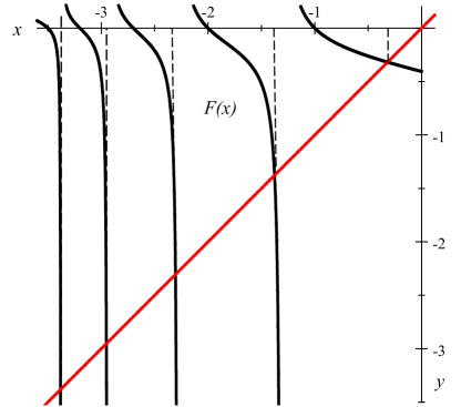
Figure 1: An example of the graphic solution of Eq. (46). Solid curves show $p$ isolated segments of $y=F(x)$, where $p$ vertical dashed lines mark $x=b_{j}$. All $p$ solutions of Eq. (46) correspond to the intersections of the solid curves with the diagonal red line $y=x$. The total number of ion species ($p=5$) and the specific values of $a_{j}$ used in this example serve only to illustrate the general behavior of the solutions; they do not correspond to any real physical situation in the solar chromosphere or elsewhere.

All $p$ roots of $\zeta_{e}=F(\zeta_{e})$ are given by the intersections of the diagonal $y=\zeta_{e}$ with the curve $y=F(\zeta_{e})$. For any integer $p>1$, the entire curve $y=F(\zeta_{e})$ represents $p$ isolated segments $y=F_{s}(\zeta_{e})$, separated by $p-1$ singularities of the $1/(\zeta_{e}-b_{s})$-kind (bear in mind that $b_{s}\neq a_{s}$). The vertical values of each segment boundary span the entire $(-\infty,\infty)$ range of the $y$-value, either in semi-infinite $\zeta_{e}$ domains (for the two edge segments) or within finite domains between two adjacent singularities. Each singularity, $\zeta_{e}=b_{s}$, in turn, is situated between two adjacent zeroes of $F(\zeta_{e})$, $(\zeta_{e})_{s}=a_{s}$ and $(\zeta_{e})_{s+1}=a_{s+1}$. All $p$ zeroes of $F(\zeta_{e})$, $(\zeta_{e})_{s}=a_{s}$, as well as all $p-1$ singularities, $(\zeta_{e})_{s}=b_{s}$, are negative. This pertains to all $p$ roots $\zeta_{e}$ of equivalent Eqs. (45) and (46).

Thus, if all $\vec{k}\cdot\vec{U}_{j}=G_{j}kV_{0}$ are different then the solution of Eq. (46) has exactly $p$ negative roots of $\omega_{De}$. In the general case, these roots can be found numerically. Each root corresponds to a separate wave mode. However, we will be interested only in one solution that corresponds to the minimum instability threshold field (if there are more than one linearly unstable modes). Based on particular cases described below, we may suppose that this solution has the minimum value of $|\zeta_{e}|$ corresponding to the largest values of $\zeta_{j}=\zeta_{e}+G_{j}$.

Now we consider particular cases that will allow us to obtain explicit analytic solutions. First, if all ions are essentially unmagnetized ($\kappa_{j}\ll 1$, see above) then all $G_{j}\approx\cos\theta$, so that Eq. (45) reduces to $1+\zeta_{e}/[(\zeta_{e}+\cos\theta)\Psi]=0$ with the obvious solution

$$\zeta_{e}=-\ \frac{\Psi\cos\theta}{1+\Psi},\qquad\zeta_{j}=\frac{\cos\theta}{1+\Psi},$$

where $\Psi$ is defined by Eq. (42). This solution is equivalent to Eq. (41). However, if at least one ion species is partially magnetized, $\kappa_{j}\gtrsim 1$, then the situation is less simple.

As a second particular case, we consider partially magnetized ion species, assuming first that $\kappa_{j}\gtrsim 1$ holds for all ions (more accurate conditions will be discussed below). For partially magnetized ions, the quantities $\vec{k}\cdot\vec{V}_{j0}$ are not negligibly small. Being unable to find the general exact solution of Eq. (45) or (46), one can utilize an approximate approach, implemented earlier for the pure FBI [31]. This approach is based on the existence of a small parameter

$$\Theta_{j}\equiv\sqrt{\frac{\kappa_{j}}{\kappa_{e}}}=\sqrt{\frac{m_{e}\nu_{en}}{m_{j}\nu_{jn}}}.$$ (48)

For example, throughout the E-region ionosphere, $\Theta_{j}=\Theta_{0}\simeq 1.4\times 10^{-2}$, see Refs. 25, 8. In the solar chromosphere, dominated by ion collisions with the light atomic hydrogen, the values of $\Theta_{j}$ are typically larger (see below), but they always obey a slightly weaker inequality, $\Theta_{j}^{2}\ll 1$.

Fletcher et al. [31] used the following idea. Restricting the treatment to strictly perpendicular waves, $k_{\parallel}=0$, for which we usually expect the minimal threshold field, one can write the parameter $\psi_{j}$ defined by Eq. (37) as $\psi_{j}=\Theta_{j}^{2}/\kappa_{j}^{2}$. Then for partially magnetized ion species, assuming $\kappa_{j}^{2}\gg\Theta_{j}^{2}$, one automatically has $\psi_{j}\ll 1$. In the E-region ionosphere, at altitudes where $\psi_{j}=\psi\ll 1$ (usually, above 100 km of altitude), this automatically provides $|\zeta_{e}|\ll 1$. Expecting a similar inequality to hold for all multi-species ions in other media, one can easily solve Eq. (45) by neglecting $|\zeta_{e}|$ compared to $G_{j}$ in all denominators. This reduces the original high-order polynomial equation to a linear one with the simple (and unique) solution,

$$\zeta_{e} \approx-\left[\sum_{j=1}^{p}\frac{\rho_{j}}{(\cos\theta-\kappa_{j}\sin\theta)\psi_{j}}\right]^{-1}$$

$$=-\left[\sum_{j=1}^{p}\frac{\rho_{j}}{(1+\kappa_{j}^{2})^{1/2}\psi_{j}\cos\chi_{j}}\right]^{-1},$$ (49a)

$$\zeta_{j} \approx G_{j}=\frac{\cos\theta-\kappa_{j}\sin\theta}{1+\kappa_{j}^{2}},$$ (49b)

for each ion species $$j |\zeta_{e}|\ll|G_{j}|$$. The condition for this approximate solution, , requires

$$\left|\left[\sum_{j=1}^{p}\frac{\rho_{j}}{(\cos\theta-\kappa_{j}\sin\theta)\psi_{j}}\right]^{-1}\right|\ll\frac{|\cos\theta-\kappa_{j}\sin\theta|}{1+\kappa_{j}^{2}}.$$ (50)

Assuming both $|\cos\theta-\kappa_{j}\sin\theta|$ and $\kappa_{j}^{2}$ to be of order unity, we reduce Eq. (50) to a much simpler criterion: $\Psi\ll 1$. If the wave direction is such that for some specific ion species the flow angle $\theta$ is close to $\tan^{-1}\kappa_{j}$ (leading to $|\cos\theta-\kappa_{j}\sin\theta|\rightarrow 0$) then the corresponding contribution to the summation, $j=i$, dominates, reducing the Eq. (50) to

$$\psi_{j}=\frac{\Theta_{j}^{2}}{\kappa_{j}^{2}}\ll 1.$$ (51)

The above two cases of low-magnetized ions, $\kappa_{j}\ll 1$ (equivalent to $\psi_{j}\gg\Theta_{j}^{2}$) and the low-$\psi_{j}$ case, $\psi_{j}\ll 1$ (equivalent to $\kappa_{j}^{2}\gg\Theta_{j}^{2}$) overlap under fairly broad conditions of $\Theta_{j}^{2}\ll\psi_{j}\ll 1$, equivalent to $1\gg\kappa_{j}^{2}\gg\Theta_{j}^{2}$. These two overlapping cases together cover a significant domain of the collisional plasma parameters, but they still do not encompass all possible situations. The reason is that the relevant ion-magnetization conditions were imposed for all ions. However, there is a possibility that at a given location the conditions $\kappa_{j}\ll 1$ and $\kappa_{j}\gtrsim 1$ are satisfied separately for different ion species. In those cases, Eq. (45) does not necessarily reduce to a simple linear equation for $\zeta_{e}$. In some cases, if the ratios $\rho_{j}/\psi_{j}$ with small $\psi_{j}\ll 1$ dominate over all the others with $\psi_{j}\gtrsim 1$ then this case can be approximately reduced to the above low-$\psi_{j}$ case. If, however, the corresponding ion concentrations $\rho_{j}$ are too small, $\rho_{j}\lesssim\psi_{j}$, then the situation is more complicated.

For the solar chromosphere, however, the general situation simplifies dramatically if we assume that for both $e$-$n$ and $i$-$n$ collisions the MMC approximation holds (see Sec. III.1). In this approximation, for elastic $i$-$n$ or $e$-$n$ collisions (assuming first no charge exchange between the colliding ions and atoms of different materials), the expression for the $s$-$n$ collision frequency is given by [47, 32],

$$\nu_{sn}=\frac{2.21\pi n_{n}m_{n}}{m_{s}+m_{n}}\sqrt{\frac{\alpha_{n}e^{2}}{4\pi\epsilon_{0}\mu_{sn}}}\approx 1.96n_{n}\sqrt{\frac{\alpha_{n}e^{2}m_{n}}{\epsilon_{0}m_{s}\left(m_{s}+m_{n}\right)}},$$ (52)

where $\mu_{sn}=m_{s}m_{n}/(m_{s}+m_{n})$ is the reduced mass of the two colliding particles, $n_{n}$ is the neutral particle density, $\epsilon_{0}$ is the permittivity of free space, and $\alpha_{n}$ is the neutral-particle polarizability. In the solar chromosphere, the dominant neutral component is the atomic hydrogen (H) for which we have $\alpha_{n}\approx\alpha_{\mathrm{H}}\approx 0.67\times 10^{-24}\operatorname{cm}^{3}$, see Ref. 47.

Elastic-collision Eq. (52) applies there only to $i$-H collisions of heavy ions like C⁺, Mg⁺, Fe⁺, etc. ($s=j^{+}\neq\mathrm{H}^{+}$), whose mass is significantly larger than the atomic mass of the neutral collision partner H ($m_{n}=m_{\mathrm{H}}$; recall that here we ignore any contribution of He). For these heavy ions, one can neglect the hydrogen mass $m_{\mathrm{H}}$ compared to $m_{j^{+}}$, so that $\mu_{j^{+}\mathrm{H}}\approx m_{\mathrm{H}}$ and

$$\nu_{j^{+}\mathrm{H}}\approx 1.96n_{\mathrm{H}}\sqrt{\frac{\alpha_{\mathrm{H}}e^{2}m_{\mathrm{H}}}{\epsilon_{0}m_{j^{+}}^{2}}}\approx 2.11\times 10^{5}\ \frac{m_{\mathrm{H}}}{m_{j^{+}}}\left(\frac{n_{\mathrm{H}}}{10^{20}\operatorname{m}^{-3}}\right)\operatorname{s}^{-1}.$$ (53)

The inverse proportionality of $\nu_{j^{+}\mathrm{H}}$ to the ion mass directly follows from the fact that heavy chromospheric ions collide predominantly with the much lighter neutral atoms (H).

For the H⁺-H collisions, to a reasonable accuracy, one can also use the MMC approximation, i.e., assume nearly constant $\nu_{\mathrm{H}^{+}\mathrm{H}}$, but not the specific elastic-collision expression given by Eq. (52). Using Figure 1 from Ref. 48 (after smoothing the corresponding curve over frequent oscillations), we approximately obtain

$$\nu_{\mathrm{H}^{+}\mathrm{H}}\simeq 2\times 10^{6}\left(\frac{n_{\mathrm{H}}}{10^{20}\operatorname{m}^{-3}}\right)\operatorname{s}^{-1}.$$ (54)

Note that Eq. (52) would result in about twenty times smaller value for $\nu_{\mathrm{H}^{+}\mathrm{H}}$. The charge-exchange process is the major reason for the much higher total $\mathrm{H}^{+}$-$\mathrm{H}$ collision frequency.

For the e-H collisions, using Eq. (52), we obtain:

$$\nu_{e\mathrm{H}}\approx 1.96n_{n}\sqrt{\frac{\alpha_{n}e^{2}}{\epsilon_{0}m_{e}}}\approx 0.905\times 10^{7}\left(\frac{n_{\mathrm{H}}}{10^{20}\operatorname{m}^{-3}}\right)\operatorname{s}^{-1}.$$ (55)

Figure 4 from Ref. 48 provides a value of $\nu_{e\mathrm{H}}$ reasonably close to this.

The fact that the collision frequency $\nu_{j^{+}\mathrm{H}}$ for $j^{+}\neq\mathrm{H}^{+}$ is inversely proportional to the ion mass means that the magnetization ratio $\kappa_{j^{+}}=\Omega_{j^{+}}/\nu_{j^{+}\mathrm{H}}$ has approximately the same common value for all heavy-ion collisions with the neutral hydrogen,

$$\kappa_{i}=\kappa_{j^{+}}\approx\frac{0.51B_{0}}{n_{\mathrm{H}}}\sqrt{\frac{\epsilon_{0}}{\alpha_{\mathrm{H}}m_{\mathrm{H}}}}\approx 0.45\left(\frac{B_{0}}{10\operatorname{G}}\right)\left(\frac{10^{20}\operatorname{m}^{-3}}{n_{\mathrm{H}}}\right).$$ (56)

Due to this, for all heavy ions with $m_{j^{+}}\gg m_{\mathrm{H}}$, we have equal values of the parameter

$$\psi_{j^{+}0}=\frac{1}{\kappa_{e}\kappa_{j^{+}}}=\frac{\Theta_{i}^{2}}{\kappa_{i}^{2}},$$

where

$$\Theta_{i}\equiv\Theta_{j^{+}\neq\mathrm{H}^{+}}=\sqrt{\frac{\kappa_{j^{+}}}{\kappa_{e}}}=\sqrt{\frac{m_{e}\nu_{e\mathrm{H}}}{m_{j^{+}}\nu_{j^{+}\mathrm{H}}}}$$ (57)

with the subscript $i$ applying only to the heavy ions. For these ions, the parameter $\Theta_{i}^{2}$ is fairly small,

$$\Theta_{i}^{2}\approx\sqrt{\frac{m_{e}}{m_{\mathrm{H}}}}\approx 2.334\times 10^{-2}.$$ (58)

For the $\mathrm{H}^{+}$-$\mathrm{H}$ collision magnetization parameter, we obtain

$$\kappa_{\mathrm{H}^{+}}\approx 4.79\times 10^{-2}\left(\frac{B_{0}}{10\operatorname{G}}\right)\left(\frac{10^{20}\operatorname{m}^{-3}}{n_{\mathrm{H}}}\right).$$ (59)

This value is an order of magnitude smaller than $\kappa_{i}=\kappa_{j^{+}}$. Accordingly, $\Theta_{\mathrm{H}^{+}}^{2}$ turns out to be an order of magnitude smaller than $\Theta_{i}^{2}$,

$$\Theta_{\mathrm{H}^{+}}^{2}=\sqrt{\frac{\kappa_{\mathrm{H}^{+}}}{\kappa_{e}}}\approx 2.4646\times 10^{-3}.$$ (60)

We will use the smallness of the parameters $\Theta_{i}^{2}$ and $\Theta_{\mathrm{H}^{+}}^{2}$ below.

Thus, instead of $p$ totally different values of ion magnetization parameters, under conditions of $m_{j}\gg m_{\mathrm{H}}$ we have only two distinct values of the ion magnetization parameter: $\kappa_{i}$ for all heavy ions and $\kappa_{\mathrm{H}^{+}}$ for H⁺. As a result, Eq. (45) reduces to a much simpler equation:

$$1+\frac{\zeta_{e}\xi_{\mathrm{H}^{+}}}{\zeta_{e}+G_{\mathrm{H}^{+}}}+\frac{\zeta_{e}\xi_{i}}{\zeta_{e}+G_{j}}=0,$$ (61)

where, in accord with Eqs. (8) and (31),

$$\xi_{\mathrm{H}^{+}}\equiv\frac{\rho_{\mathrm{H}^{+}}\kappa_{\mathrm{H}^{+}}^{2}}{(1+\kappa_{\mathrm{H}^{+}}^{2})\Theta_{\mathrm{H}^{+}}^{2}}=\frac{\varepsilon\rho_{\mathrm{H}^{+}}\kappa_{i}^{2}}{(1+\varepsilon^{2}\kappa_{i}^{2})\Theta_{i}^{2}},$$

$$\xi_{i}\equiv\frac{\rho_{i}\kappa_{i}^{2}}{(1+\kappa_{i}^{2})\Theta_{i}^{2}},\qquad\rho_{i}\equiv\sum_{i^{+}\neq\mathrm{H}^{+}}\rho_{i^{+}}=1-\rho_{\mathrm{H}^{+}}.$$

$$G_{i}\equiv\frac{\vec{k}\cdot\vec{U}_{i}}{kV_{0}}=\frac{\cos\theta-\kappa_{i}\sin\theta}{1+\kappa_{i}^{2}},$$

$$G_{\mathrm{H}^{+}}\equiv\frac{\vec{k}\cdot\vec{U}_{\mathrm{H}^{+}}}{kV_{0}}=\frac{\cos\theta-\varepsilon\kappa_{i}\sin\theta}{1+\varepsilon^{2}\kappa_{i}^{2}}.$$ (62)

Here $\varepsilon$ is a small dimensionless parameter,

$$\varepsilon\equiv\frac{\kappa_{\mathrm{H}^{+}}}{\kappa_{i}}=\frac{\Theta_{\mathrm{H}^{+}}^{2}}{\Theta_{i}^{2}}\approx 0.1056.$$ (63)

According to Eq. (62), given constant $k$, $\theta$, $V_{0}$, $\rho_{\mathrm{H}^{+}}$ and the small parameters $\Theta_{i}^{2}$ and $\varepsilon$ defined by Eqs. (58) and (63), all remaining quantities in Eq. (61) are expressed in terms of only one parameter, $\kappa_{i}^{2}$, which varies with the total hydrogen density and magnetic field according to Eq. (56).

In an obvious way, Eq. (61) reduces to a quadratic equation for $\zeta_{e}=\omega_{De}/(kV_{0})$,

$$(1+\xi_{\mathrm{H}^{+}}+\xi_{i})\zeta_{e}^{2}+[(1+\xi_{\mathrm{H}^{+}})G_{i}+(1+\xi_{i})G_{\mathrm{H}^{+}}]\zeta_{e}+G_{\mathrm{H}^{+}}G_{i}=0,$$ (64)

whose two exact roots, $\zeta_{e}^{(1,2)}$, can be written as

$$\zeta_{e}^{(1)} =-\ \frac{2G_{\mathrm{H}^{+}}G_{i}}{(1+\xi_{\mathrm{H}^{+}})G_{i}+(1+\xi_{i})G_{\mathrm{H}^{+}}+Z}\,,$$ (65a)

$$\zeta_{e}^{(2)} =-\ \frac{(1+\xi_{\mathrm{H}^{+}})G_{i}+(1+\xi_{i})G_{\mathrm{H}^{+}}+Z}{2(1+\xi_{i}+\xi_{\mathrm{H}^{+}})}\,,$$ (65b)

where

$$Z=\sqrt{[(1+\xi_{\mathrm{H}^{+}})G_{i}-(1+\xi_{i})G_{\mathrm{H}^{+}}]^{2}+4\xi_{\mathrm{H}^{+}}\xi_{i}G_{\mathrm{H}^{+}}G_{i}}\,.$$ (66)

We have written the two roots of a quadratic equation in an unconventional, but equivalent, form which makes perfectly clear that each solution for $\zeta_{e}$ is real and negative. Besides, in the large-$\xi_{i,\mathrm{H}}$ limit (see below), the conventional form of the solution for $\zeta_{e}^{(1)}$ would result in subtraction of two major terms, while Eq. (65a) allows one to avoid that.

The above exact solution of simplified Eq. (64) remains complicated for analysis. Below, using the specific parameter relations found above, we will construct a much simpler, but still reasonably accurate, approximate solution.

First, assuming $\kappa_{i}^{2}\ll 1$, so that automatically $\kappa_{\mathrm{H}^{+}}^{2}=\varepsilon^{2}\kappa_{i}^{2}\ll 1$, we reduce this case to the fully unmagnetized case described above. In the specific case of $\vec{U}_{j}\approx\vec{U}_{\mathrm{H}^{+}}\approx\vec{V}_{0}$, Eq. (61) yields

$$\omega_{De}\approx-\ \frac{\vec{k}\cdot\vec{V}_{0}}{1+\xi_{i}+\xi_{\mathrm{H}^{+}}}.$$ (67)

For $\vec{U}_{j}\approx\vec{U}_{\mathrm{H}^{+}}\approx\vec{V}_{0}$, this solution also follows from Eq. (65a).

Now we consider a broader span of the ion magnetization parameters that includes $\kappa_{i}^{2}\gtrsim 1$. In this, more general, case, one should no longer expect $\vec{U}_{j}\approx\vec{U}_{\mathrm{H}^{+}}\approx\vec{V}_{0}$, though $|\vec{U}_{j}|$ and $|\vec{U}_{\mathrm{H}^{+}}|$ usually have comparable values. Indeed, only for strongly magnetized ions, $\kappa_{i}^{2}\gg 1$, while $\varepsilon^{2}\kappa_{i}^{2}\lesssim 1$, we would have $|\vec{U}_{j}|\ll|\vec{U}_{\mathrm{H}^{+}}|\sim V_{0}$, but this case is of no interest to us because the large-$\kappa_{i}^{2}$ is linearly stable, as discussed above. In all other cases, we typically have $|\vec{U}_{j}|\sim|\vec{U}_{\mathrm{H}^{+}}|\sim V_{0}$. Assuming in Eq. (61) $|\zeta_{e}|$ to be small compared to $G_{j}\sim G_{\mathrm{H}^{+}}$ (the condition will be discussed below) and neglecting $\zeta_{e}$ in both denominators, we obtain

$$\zeta_{e}\approx-\left(\frac{\xi_{i}}{G_{j}}+\frac{\xi_{\mathrm{H}^{+}}}{G_{\mathrm{H}^{+}}}\right)^{-1}.$$ (68)

From Eq. (68), assuming $G_{\mathrm{H}^{+}}\sim G_{j}$, we obtain that the presumed condition of $|\zeta_{e}|\ll G_{\mathrm{H}^{+}}\sim G_{j}$ requires $\xi_{i,\mathrm{H}^{+}}\gg 1$. It can be easily verified that the approximate solution given by (68) follows from Eq. (65a) if one neglects the “unity” compared to both $\xi_{\mathrm{H}^{+}}$ and $\xi_{i}$. According to Eq. (62), unless the fraction of heavy ions is too small ($\rho_{i}\lesssim\Theta_{i}^{2}\simeq 0.02$), the condition of $\xi_{i}\sim\rho_{i}\kappa_{i}^{2}/\Theta_{i}^{2}\gg 1$ is automatically fulfilled for $\kappa_{i}^{2}\sim 1$. Similarly, unless $\rho_{\mathrm{H}^{+}}$ is too small ($\rho_{\mathrm{H}^{+}}\lesssim\Theta_{i}^{2}/\varepsilon\simeq 0.2$), the condition $\xi_{\mathrm{H}^{+}}\sim\varepsilon\rho_{\mathrm{H}^{+}}\kappa_{i}^{2}/\Theta_{i}^{2}\gg 1$ is also automatically fulfilled for the same range of $\kappa_{i}^{2}\sim 1$. In principle, if $\rho_{\mathrm{H}^{+}}\lesssim 0.2$ then $\xi_{\mathrm{H}^{+}}\lesssim 1$, so that $1$ cannot be dropped compared to $\xi_{\mathrm{H}^{+}}$. However, this does not really matter since the corresponding second term, $\xi_{\mathrm{H}^{+}}/G_{\mathrm{H}^{+}}$, in Eq. (68) is small in itself (compared to the first term, $\xi_{i}/G_{j}$). The inaccuracy of this small term is largely inconsequential.

The two approximate solutions given by Eqs. (67) and (65) match within the overlap range of $\Theta_{i}^{2}/\rho_{i}\ll\kappa_{i}^{2}\ll 1$, where both conditions of $G_{\mathrm{H}^{+}}\approx G_{j}\approx\cos\theta$ and $\xi_{i}\gg 1$ are fulfilled simultaneously. For the most interesting cases, one can construct an interpolation between the two solutions, using the simple ansatz:

$$\zeta_{e}\approx-\left(\frac{\alpha_{1}+\xi_{i}}{G_{j}}+\frac{1-\alpha_{1}+\xi_{\mathrm{H}^{+}}}{G_{\mathrm{H}^{+}}}\right)^{-1},$$ (69)

where the specific value of the numeric parameter $\alpha_{1}$ can be chosen between 0 and 1. This simple interpolation works well mostly within the range of flow angles $\theta$ between $-45^{\circ}$ (the optimal angle for the pure ETI) and $0^{\circ}$ (the optimal angle for the pure FBI).

Figure 2: Solution of Eq. (61) given by Eq. (65a) for three values of the flow angle $\theta$ (the solid curves) and for five different values of the heavy-ion fraction, $\rho_{i}=1-\rho_{\mathrm{H}^{+}}$, along with the corresponding interpolations given by Eq. (69) and described in the text (the dashed curves). In the interpolation curves, the red, yellow, and green curves correspond to $\alpha_{1}$ equal to 0, 0.5, and 1, respectively.

Figure 2 shows the solution of Eq. (61) given by Eq. (65a) for three values of the flow angle $\theta$. This solution (normalized to $kV_{0}$) is shown by solid curves for five different values of the heavy-ion fraction, $\rho_{i}=1-\rho_{\mathrm{H}^{+}}$ (shown near the curves). Around these curves, there also interpolations given by Eq. (69) (shown by the dashed color curves) for three different values of the fitting parameter $\alpha_{1}$ ($\alpha_{1}=0$, $0.5$, $1$). For $\theta=-0^{\circ}$ and $\theta=-22.5^{\circ}$, the ansatz of Eq. (69) works reasonably well with any values of $\alpha_{1}$, so that for $\rho_{i}\gtrsim 0.25$, the interpolations are almost indistinguishable from the exact solution. For $-22.5^{\circ}\lesssim\theta\leq 0^{\circ}$, the interpolation works reasonably well for all values $\rho_{i}$, even for $\rho_{i}$ as low as $0.02$. For $\theta=-45^{\circ}$, the interpolation starts deviating from the exact solution, though the specific value of $\alpha_{1}$ matters only for low concentrations, $\rho_{i}<0.1$, and mostly for low-magnetized ions, $\kappa_{i}<0.5$. Generally, for most interesting cases of $\theta$ within $-45^{\circ}$ to $0^{\circ}$ range, the choice of $\alpha_{1}=1-\alpha_{1}=0.5$ seems to be optimal. For all these cases, Eq. (69) can serve as a reasonably accurate and a more practical alternative to the cumbersome exact solution given by Eq. (65). Unfortunately, for angles beyond the domain of $-45^{\circ}\lesssim\theta\leq 0^{\circ}$, the simple interpolation of Eq. (69) often does not work well, so that one needs to apply there the full solution given by Eq. (65a).

In this analysis, we have considered only one root of Eq. (64), namely $\zeta_{e}=\zeta_{e}^{(1)}$. The reason is that only this root provides an accurate transition to the well-established SSI solution. The other root, $\zeta_{e}=\zeta_{e}^{(2)}$ has no SSI analog. Besides, the corresponding value of $\zeta_{i}=\zeta_{e}^{(2)}+G_{i}$ becomes fairly small and inefficient for driving the instabilities (see below).

To conclude this section, we note that in the long-wavelength limit, the highest-order approximation to the reduced dispersion relation (34) describes the linear wave phase velocity relation

$$\omega_{r}\approx\vec{k}\cdot\vec{V}_{0}+\omega_{De}(\vec{k})=\left[\cos\theta+\zeta_{e}(\theta)\right]kV_{0}.$$ (70)

where $\zeta_{e}$ is the proper solution of Eq. (45) discussed above. In the LWL, this relation is common for all stable or unstable waves, whatever the specific mechanism of wave generation. Notice the linear $k$-scaling of the real wave frequency (and hence of all Doppler-shifted frequencies, $\omega_{Ds}$). The next-order approximation provides the instability growth/damping rates, which are different for different physical mechanisms. The corresponding analysis will be performed in the following section.

V.2 First-order approximation: instability growth/damping rates. Different physical mechanisms

To determine specific mechanisms of instability generation, we need to consider the next, i.e., first-order, approximation with respect to the small parameters $\left|A_{e,j}\right|,\left|B_{e,j}\right|,k_{\parallel}^{2}/k_{\perp}^{2},k^{2}\lambda_{D}^{2}$ introduced by Eq. (33). To find the instability growth/damping rates, $|\gamma|\ll\omega_{r}$, according to Eq. (35), we need to linearize the RHS of Eq. (34) with respect to the above small parameters and retain only the imaginary part of $D(\omega,\vec{k})$. (The real part of the first-order term in the Taylor expansion of $D(\omega,\vec{k})$ will provide just a small correction to the wave phase velocity relation and will be of no interest to us.) Given the known solution for $\omega_{De}(\vec{k})=\zeta_{e}(\theta)kV_{0}$, and hence for all $\omega_{Dj}(\vec{k})=\omega_{De}+\vec{k}\cdot\vec{U}_{j}=[\zeta_{e}(\theta)+G_{j}(\theta)]kV_{0}$, finding the growth/damping rates becomes a straightforward procedure.

We start by calculating the denominator in the RHS of Eq. (35). According to Eq. (36) and (38), where $\omega_{De}$ and all $\omega_{Dj}$ are known functions of $\omega\approx\omega_{r}$ determined to the leading (zeroth-order) accuracy (see above), we obtain:

$$\frac{\partial D_{0}(\omega_{r},\vec{k})}{\partial\omega_{r}}=\sum_{j=1}^{p}\frac{\rho_{j}(\vec{k}\cdot\vec{U}_{j})}{(1+\kappa_{j}^{2})\omega_{Dj}^{2}\psi_{j}}.$$ (71)

Calculating the numerator in the RHS of Eq. (35), i.e., $\operatorname{Im}D(\omega,\vec{k})$, is a more cumbersome procedure. In the RHS of Eq. (34), the standalone terms $\propto A_{s}$, $B_{s}$ given by Eqs. (27)–(31) are small and can be used to the leading-order accuracy, while the ratio $A_{j}/B_{j}$ requires a better accuracy. Neglecting small terms $\propto i\omega_{De}/\nu_{en}$, but keeping the first-order approximation with respect to $\left|\Omega_{j}\right|/\nu_{jn}=|\omega-\vec{k}\cdot\vec{V}_{j}|/\nu_{jn}$, and bearing in mind that usually $\nu_{en}\gg\nu_{jn}$, we obtain

$$\frac{\alpha_{j}A_{j}}{A_{e}} \approx\frac{\omega_{De}\kappa_{e}^{2}\nu_{en}m_{e}(1-i\omega_{Dj}/\nu_{jn})}{\omega_{Dj}\nu_{jn}m_{i}(1+\kappa_{e}^{2}k_{\parallel}^{2}/k_{\perp}^{2})[\left(1-i\omega_{Dj}/\nu_{jn}\right)^{2}+\kappa_{j}^{2}]}$$

$$\approx\frac{\omega_{De}}{\omega_{Dj}\psi_{j}(1+\kappa_{j}^{2})}\left(1+i\ \frac{1-\kappa_{j}^{2}}{1+\kappa_{j}^{2}}\frac{\omega_{Dj}}{\nu_{jn}}\right),$$

so that

$$\operatorname{Im}\left(1+\sum_{j=1}^{p}\frac{\rho_{j}\alpha_{j}A_{j}}{A_{e}}\right)\approx\sum_{j=1}^{p}\frac{(1-\kappa_{j}^{2})\rho_{j}\omega_{De}}{(1+\kappa_{j}^{2})^{2}\nu_{jn}\psi_{j}}.$$ (72)

Substituting Eq. (72) into Eq. (71) and slightly redistributing the terms in the RHS of Eq. (35), we obtain the following interim expression for the instability growth rate:

$$\gamma\approx-\ \frac{\omega_{De}}{\sum_{j=1}^{p}\left.\rho_{j}(\vec{k}\cdot\vec{U}_{j})\right/[(1+\kappa_{j}^{2})\omega_{Dj}^{2}\psi_{j}]}\sum_{j=1}^{p}\frac{\rho_{j}}{\left(1+\kappa_{j}^{2}\right)\omega_{Dj}\psi_{j}}$$

$$\times\left\{\frac{\omega_{Dj}}{\nu_{j}}\left[\overset{\mathrm{Farley-Buneman}}{\overbrace{\frac{1-\kappa_{j}^{2}}{1+\kappa_{j}^{2}}}}-\overset{\text{{Charge }}\mathrm{Separation}}{\overbrace{\frac{\left(1+\kappa_{j}^{2}\right)\nu_{jn}^{2}}{\omega_{pj}^{2}}}}\right]+~{}\overset{\mathrm{Diffusion}\text{ Losses}}{\overbrace{\operatorname{Im}\left(A_{j}-A_{e}\right)}}~{}\right.$$

$$+~{}\left.\overset{\mathrm{Ion}\text{ }\mathrm{Thermal}}{\overbrace{\operatorname{Im}\frac{1}{\mu_{j}}\left(\frac{2A_{j}}{3}+B_{j}\right)}}\overset{\mathrm{Electron}\text{ }\mathrm{Thermal}}{~{}-~{}\overbrace{\operatorname{Im}\frac{1}{\mu_{e}}\left(\frac{2A_{e}}{3}+B_{e}\right)}}\right\}$$

$$=\gamma_{\mathrm{FB}}-\gamma_{\mathrm{CS}}+\gamma_{\mathrm{DL}}+\gamma_{\mathrm{IT}}+\gamma_{\mathrm{ET}},$$ (73)

where $\omega_{pj}\equiv\left({e^{2}n_{e0}}/{\epsilon_{0}m_{j}}\right)^{1/2}$ is the plasma frequency of the $j$-th ion species. The labels over the braces, along with the corresponding acronyms in the subscripts at the bottom line of Eq. (73), show the physical interpretation of each term. They have a straightforward meaning. The Farley-Buneman (“FB”) instability term originates from Eq. (72). The label “Charge Separation” (“CS”) means a small deviation from quasi-neutrality; the corresponding term stems from the $k^{2}\lambda_{D}^{2}/A_{e}$ term in the RHS of Eq. (34), though without the corresponding multiplier in the square bracket (the terms $\propto A_{e}$ and $B_{e}$ multiplied by $k^{2}\lambda_{De}^{2}/A_{e}$ would lead to negligibly small, second-order corrections). The label “Diffusion Losses” (“DL”) denotes the diffusion losses caused by density gradients formed within the given compression/rarefaction wave. Depending on the parameters and wave characteristics, the “FB”, “ET”, and “IT” mechanisms are responsible for driving the FBI, ETI, and ITI, respectively, while the “DL” and “CS” are stabilizing (damping) mechanisms.

Before proceeding with the explicit expressions for the above terms, we briefly discuss the physical mechanisms behind the wave damping and instabilities. We start by discussing the wave damping mechanisms. The major of the damping mechanisms, the diffusion losses of given particles of species $s$ are caused by the ambipolar diffusion of the particles from the wave density crests to the nearby wave troughs. This plasma particle diffusion is caused by the wave spatial gradients of the regular particle pressure, $\nabla(n_{s}T_{s})\propto i\vec{k}T_{s0}\delta n_{s}$ (assuming for simplicity the isothermal regime). Within a given density wave, the particle diffusion is always stabilizing. In the absence of instability excitation mechanisms, the particle diffusion would eventually smear out any initially created wave density perturbations, leading to the total wave disappearance. The linear instability means that there should exist some physical mechanisms that are able to reverse the stabilizing effect of the ambipolar diffusion and lead to an exponential growth of the initial small wave perturbation. For a physical explanation of the charge separation (CS) effect, see the appendix of Ref. 50.

Now we briefly discuss the instability driving mechanisms. The FBI is driven by the ion inertia. In the wave frame of reference, this inertia, through the $m_{s}(\vec{V}_{s}\cdot\nabla)\vec{V}_{s}$-term hidden within the $m_{s}D_{s}\vec{V}_{s}/Dt$-term of Eq. (1b), creates an additional “kinetic” pressure perturbation, $m_{s}(\vec{V}_{s}\cdot\nabla)\vec{V}_{s}\rightarrow\nabla(m_{s}V_{s}^{2}/2)\propto im_{s}\vec{k}\cdot(\vec{V}_{s}-\vec{V}_{\mathrm{ph}})\delta\vec{V}_{s}$, where $\vec{V}_{\mathrm{ph}}$ is the wave phase velocity. For sufficiently strong driving electric field, $\vec{E}_{0}$, and properly oriented (with respect to $\vec{E}_{0}$ and $\vec{B}_{0}$) wavevector $\vec{k}$, this additional pressure may be in antiphase to the wave perturbation of the regular plasma pressure $\propto T_{s0}\delta n_{s}$, overpower the latter, and hence drive the linear instability.

For the two thermal-driven instabilities, ETI and ITI, the additional pressure is created by wave modulations of the total ohmic heating described by the first term in the RHS of Eq. (1c). The modulated heating of plasma particles is caused by the wave electrostatic field, $\delta\vec{E}$. Balanced by collisional cooling, this heating leads to local modulations of the corresponding species temperature, $\delta T_{s}$. Similarly to the FBI, for the properly oriented wavevector $\vec{k}$, the additional pressure $\propto n_{s0}\delta T_{s}$ may reverse the sign of the total wave pressure perturbation $\propto(T_{s0}\delta n_{s}+n_{s0}\delta T_{s})$ and drive the instability.

The explicit expressions for the specific partial growth/damping rates, calculated to the leading-order accuracy, are given by

$$\gamma_{\mathrm{FB}}-\gamma_{\mathrm{CS}}$$

$$=\left.\sum_{j=1}^{p}\frac{\rho_{j}(-\omega_{De})}{(1+\kappa_{j}^{2})\nu_{jn}\psi_{j}}\left[\frac{1-\kappa_{j}^{2}}{1+\kappa_{j}^{2}}-\frac{(1+\kappa_{j}^{2})\nu_{jn}^{2}}{\omega_{pj}^{2}}\right]\right/\sum_{j=1}^{p}\frac{\rho_{j}(\vec{k}\cdot\vec{U}_{j})}{(1+\kappa_{j}^{2})\omega_{Dj}^{2}\psi_{j}},$$ (74a)

$$\gamma_{\mathrm{DL}}=\left.-\sum_{j=1}^{p}\frac{\rho_{j}k^{2}V_{Tj}^{2}}{(1+\kappa_{j}^{2})\omega_{Dj}\psi_{j}\nu_{jn}}\ \left[\frac{T_{e0}\psi_{j}}{T_{j0}}-\frac{\omega_{De}}{(1+\kappa_{j}^{2})\omega_{Dj}}\right]\right/\sum_{j=1}^{p}\frac{\rho_{j}(\vec{k}\cdot\vec{U}_{j})}{(1+\kappa_{j}^{2})\omega_{Dj}^{2}\psi_{j}},$$ (74b)

$$\gamma_{\mathrm{IT}}=$$

$$=\left.\sum_{j=1}^{p}\frac{4m_{n}}{3(m_{j}+m_{n})}\ \frac{\rho_{j}(-\omega_{De})\kappa_{j}kU_{j}(\kappa_{j}\cos\chi_{j}-\sin\chi_{j})}{(1+\kappa_{j}^{2})^{2}\omega_{Dj}\psi_{j}\delta_{jn}\nu_{jn}}\right/\sum_{j=1}^{p}\frac{\rho_{j}(\vec{k}\cdot\vec{U}_{j})}{(1+\kappa_{j}^{2})\omega_{Dj}^{2}\psi_{j}},$$ (74c)

$$\gamma_{\mathrm{ET}}=\frac{4kV_{0}\delta_{en}\nu_{en}\sin\theta}{3(\omega_{De}^{2}+\delta_{en}^{2}\nu_{en}^{2})\kappa_{e}}$$

$$\times\left.\sum_{j=1}^{p}\frac{\rho_{j}\omega_{De}}{(1+\kappa_{j}^{2})\omega_{Dj}\psi_{j}}\left(1-\frac{T_{e0}kV_{Tj}^{2}\omega_{De}\psi_{j}\kappa_{e}}{2T_{j0}\nu_{jn}V_{0}\delta_{en}\nu_{en}\sin\theta}\right)\right/\sum_{j=1}^{p}\frac{\rho_{j}(\vec{k}\cdot\vec{U}_{j})}{(1+\kappa_{j}^{2})\omega_{Dj}^{2}\psi_{j}},$$ (74d)

where the angles $\chi_{j}(\theta)$ are defined by Eq. (31). As discussed in Sec. V.1, for any allowed linear-wave modes, $\omega_{De}$ is always negative, while all corresponding $\omega_{Dj}=\omega_{De}+\vec{k}\cdot\vec{U}_{j}$ are positive. The diffusion loss rate, $\gamma_{\mathrm{DL}}$, is always negative, whereas in order to drive the FBI ($\gamma_{\mathrm{FB}}-\gamma_{\mathrm{CS}}>0$) the square bracket in the RHS of Eq. (74a) has to be positive.

In Eq. (74a), we have combined the Farley-Buneman driving mechanism ($\gamma_{\mathrm{FB}}$, see the first term in the square brackets) with the charge-separation losses ($\gamma_{\mathrm{CS}}$, see the second term in the square brackets) in order to emphasize the possible detrimental effect of small deviations from quasi-neutrality on the FBI [51]. In the Earth’s ionosphere, due to a sufficiently high plasma density, the CS effect is usually negligible ($\nu_{jn}^{2}\ll\omega_{pj}^{2}$), although it always should be taken into account in PIC simulations [43]. In the solar chromosphere, we cannot exclude the efficiency of the CS effect in some regions. For a sufficiently low plasma density leading to $\nu_{jn}^{2}>\omega_{pj}^{2}$, the FBI cannot be excited regardless of the imposed electric-field strength. The finite ion magnetization, $\kappa_{j}^{2}\gtrsim 1$, only aggravates the situation, especially for $\kappa_{j}^{2}>1$, when even the FBI mechanism itself becomes stabilizing [8]. For other instabilities, the ITI and ETI, the CS effect increases the instability threshold, but it is not totally detrimental, regardless of the ratio $\nu_{jn}/\omega_{pj}$.

Being interested mostly in the minimal instability threshold, we can simplify our treatment further by extending the assumed LWL to even longer wavelengths that obey stronger conditions:

$$kU_{j},|\omega_{Ds}|\ll\delta_{en}\nu_{en}.$$ (75)

Usually $\delta_{en}\nu_{en}\ll\nu_{jn}$, so that the wavelengths obeying these conditions are typically much longer than those defining the LWL, see Eq. (32). We will name the new limit imposed by Eq. (75) the superlong-wavelength limit (SLWL). In accord with the SLWL conditions, we can neglect in Eq. (74d) $\omega_{De}^{2}$ compared to $\delta_{en}^{2}\nu_{en}^{2}$, as well as the second term in the first-summation parentheses compared to $1$. This will minimize the threshold-field value along any given $\vec{k}$-direction (i.e., for given $\theta$). According to zeroth-order Eq. (36), the remaining summation in the numerator of Eq. (74d) equals $-1$, so that in the SLWL $\gamma_{\mathrm{ET}}$ reduces to a much simpler expression,

$$\gamma_{\mathrm{ET}}\approx-\ \left.\frac{4kV_{0}\sin\theta}{3\delta_{en}\nu_{en}\kappa_{e}}\right/\sum_{j=1}^{p}\frac{\rho_{j}(\vec{k}\cdot\vec{U}_{j})}{(1+\kappa_{j}^{2})\omega_{Dj}^{2}\psi_{j}}.$$ (76)

Now we check the SSI case, $p=1$ ($j\rightarrow i$). In that case, Eq. (74b) rate reduces to

$$\gamma_{\mathrm{DL}}=-\ \frac{\omega_{Di}k^{2}V_{Ti}^{2}}{(\vec{k}\cdot\vec{U}_{i})\nu_{in}}\left[\frac{T_{e}\psi_{i}}{T_{i}}-\frac{\omega_{De}}{(1+\kappa_{i}^{2})\omega_{Di}}\right].$$ (77)

Using the expressions for $\omega_{De,i}$ from Eq. (38) and combining Eq. (77) with similarly calculated $\gamma_{\mathrm{FB}}$ and $\gamma_{\mathrm{CS}}$ we obtain the SSI expression for the combined growth/damping rate which includes no thermal driving:

$$\gamma_{\mathrm{FB}}-\gamma_{\mathrm{CS}}+\gamma_{\mathrm{DL}}$$

$$\!=\frac{\psi_{i}\omega_{Di}^{2}}{[1+(1+\kappa_{i}^{2})\psi_{i}]\nu_{in}}\left[1-\kappa_{i}^{2}-\frac{k_{\perp}^{2}C_{s}^{2}}{\omega_{Di}^{2}}-\frac{(1+\kappa_{i}^{2})^{2}\nu_{in}^{2}}{\omega_{pi}^{2}}\right]\!\!,$$ (78)

where $\omega_{Di}=\vec{k}\cdot\vec{U}_{i}/[1+\left(1+\kappa_{i}^{2}\right)\psi_{i}]$, while $C_{s}$ is the isothermal ion-acoustic speed defined by Eq. (11). Equation (78) agrees with the previous results for the arbitrary ion magnetization, see, e.g., Eq. (6) from Ref. 25, except for the last term in the square brackets which generalizes the CS term from Ref. 51 to $\kappa_{i}^{2}\sim 1$.

Now we note that in the SLWL all driving/damping rates $\gamma_{\mathrm{s}}$, except $\gamma_{\mathrm{ET}}$ (see below), have a simple quadratic $k$-scaling: $\gamma_{\mathrm{s}}\propto k^{2}$. To establish this, it is sufficient to assume the linear $k$-dependence of $\omega_{r}\propto k$. This is clear from $\omega_{Ds}\propto k$, in full consistency with Eq. (36) and its solutions (discussed in Sec. V.1). Setting $\omega_{Ds}\propto k$ in Eq. (74) with Eq. (74d) replaced by Eq. (76), one can easily establish the $\gamma_{s}\propto k^{2}$ scaling. This common scaling for all $\gamma_{\mathrm{s}}=0$ automatically makes the threshold field along the given $\vec{k}$-direction to be $k$-independent – the well-established fact for the pure FBI in the LWL fluid-model approximation, see, e.g., Refs. 52, 53. If the FBI is the dominant instability driver, as in most of the E-region ionosphere, then within the entire LWL the growth rate $\gamma\propto k^{2}$, so that its maximum is usually reached beyond the LWL (see also Appendix A).

If the dominant instability driver is the ETI, as we observed in our recent PIC simulations for some solar chromosphere parameters [32], then the growth rate maximum is reached within the LWL due to the competition between the two terms within the parentheses under the first summation in Eq. (74d). In the SSI case of pure ETI driving, we have

$$\gamma_{\mathrm{ET}}\approx-\ \frac{(1+\kappa_{i}^{2})\psi_{i}(\vec{k}\cdot\vec{U}_{i})}{[1+(1+\kappa_{j}^{2})\psi_{i}]^{2}}\frac{4kV_{0}\delta_{en}\nu_{en}\sin\theta}{3(\omega_{De}^{2}+\delta_{en}^{2}\nu_{en}^{2})\kappa_{e}}\left(1-\frac{T_{e}k\omega_{De}V_{Ti}^{2}\psi_{i}\kappa_{e}}{2T_{i}\nu_{in}V_{0}\delta_{en}\nu_{en}\sin\theta}\right).$$ (79)

The first term in parentheses (i.e., $1$) reflects the local heating-cooling balance, which is the crucial factor for the ETI. The second term $\propto k\omega_{De}\propto k^{2}$ is responsible for the nonlocal temperature spread within the wavelength due to the heat advection. Since $\omega_{De}$ is negative (see Sec. V.1), total $\gamma_{\mathrm{ET}}$ can be positive for some $\vec{k}$ within the negative sector, while for $\vec{k}$ within the positive sector of $\theta$, the rate $\gamma_{\mathrm{ET}}$ is always negative, regardless of the $E_{0}$ value. In the SLWL of $kU_{j}$, $\omega_{Ds}\ll\delta_{en}\nu_{en}$, neglecting $\kappa_{i}^{2}\psi_{i}$, and taking $\vec{U}_{i}\approx\vec{V}_{0}$ (assuming also $\kappa_{i}^{2}\ll 1$), we obtain a much simpler relation:

$$\gamma_{\mathrm{ET}}\simeq-\ \frac{4\psi_{i}k^{2}V_{0}^{2}\sin\theta\cos\theta}{3\left(1+\psi_{i}\right)^{2}\kappa_{e}\delta_{en}\nu_{en}}.$$ (80)

For $m_{n}=m_{i}$, $\delta_{i}=1$, $(1+\kappa_{i}^{2})\psi_{i}\rightarrow\psi_{i}$, and bearing in mind that $\kappa_{i}^{2}\psi_{i}=\kappa_{i}/\kappa_{e}\ll 1$, Eq. (81) agrees with Eq. (30) from Ref. 8. To the accuracy of the factor of order unity, this agrees with the previous results, see, e.g., Eq. (38) from Ref. 8, neglecting the term $\propto S^{2}$ originated there from the electron-temperature dependence of $\nu_{en}$. Recall that, assuming elastic $e$-$n$ collisions determined mostly by the electron polarization of the colliding neutral particle, in this paper we ignore any temperature dependence of $\nu_{en}$. We note that ignoring the $\propto S^{2}$ term leads to the absence of the additional destabilizing ETI mechanism, which is, unlike that in Eq. (80), symmetric with respect to the sign of $\theta$, see Refs. 3, 4.

Finally, we check the SSI case for the ion thermal driving. In the SSI case, Eq. (74c) reduces to

$$\gamma_{\mathrm{IT}}\approx\frac{4\psi_{i}k^{2}U_{i}^{2}m_{n}(\kappa_{i}\cos\chi_{i})(\kappa_{i}\cos\chi_{i}-\sin\chi_{i})}{3[1+(1+\kappa_{i}^{2})\psi_{i}]^{2}(m_{n}+m_{i})\delta_{in}\nu_{in}},$$ (81)

which also agrees with the previous results [8].

V.3 Threshold electric field

The threshold electric field for the combined instability (the FBI, ETI, and ITI) is determined by equating the total growth rate to zero,

$$\gamma\equiv\gamma_{\mathrm{FB}}-\gamma_{\mathrm{CS}}+\gamma_{\mathrm{DL}}+\gamma_{\mathrm{IT}}+\gamma_{\mathrm{ET}}=0.$$ (82)

where all $\gamma_{\mathrm{S}}$ are given by Eq. (74). For a given wave mode determined by its wavevector $\vec{k}$, we have obtained above the zeroth-order solution for the real negative electron Doppler-shifted frequency $\omega_{De}\approx\omega_{Der}=\zeta_{e}kV_{0}$, see Eq. (65a) or its simplified versions given by Eqs. (67)-(69). The parameters in these solutions are expressed in terms of $\vec{k}\cdot\vec{U}_{j}=G_{j}kV_{0}$, where $G_{j}$ is defined in Eq. (43), and $kU_{j}=kV_{0}/(1+\kappa_{j}^{2})^{1/2}$, see Eq. (7) and (8), i.e., eventually, in terms of the driving-field amplitude, $E_{0}=V_{0}B_{0}$ and the wavevector $\vec{k}$. Then the quantities $\omega_{Dj}=\left(\zeta_{e}+G_{j}\right)kV_{0}$, involved in all $\gamma_{\mathrm{S}}$, become also functions of $E_{0}$. Given $\vec{k}$ and the proper solution for $\zeta_{e}$, by solving Eq. (82) we obtain the instability threshold $E_{0}=E_{\mathrm{Thr}}$. Bearing in mind the minimal threshold fields, we will restrict our further treatment of wavelengths to the SLWL, in which the scaling $\gamma\propto k^{2}$ holds for all instability driving and loss mechanisms. This will allow us to cancel all $k$-related factors and obtain the general, $k$-independent, minimum value of the threshold field. While the $k$-dependence of $E_{\mathrm{Thr}}$ disappears, the dependence on the $\vec{k}$ angles still holds and is crucial. Note that total absence of real positive roots for $E_{\mathrm{Thr}}$ within a given parameter domain means the linearly stable regime, regardless of the strength of the imposed electric field $\vec{E}_{0}$.

To apply Eq. (82), we express $\omega_{De,j}$, $\vec{k}\cdot\vec{U}_{j}$ and $U_{j}=V_{0}/(1+\kappa_{j}^{2})^{1/2}$ in terms of $\zeta_{e}$ and $V_{0}$. Leaving out in Eq. (74) the inconsequential common denominator $\sum_{j=1}^{p}\rho_{j}(\vec{k}\cdot\vec{U}_{j})/[(1+\kappa_{j}^{2})\omega_{Dj}^{2}\psi_{j}]$, along with the remaining $k$-factor, we obtain

$$\gamma_{\mathrm{FB}}-\gamma_{\mathrm{CS}}\propto-V_{0}\zeta_{e}\sum_{j=1}^{p}\frac{\rho_{j}}{(1+\kappa_{j}^{2})\psi_{j}\nu_{jn}}\left[\frac{1-\kappa_{j}^{2}}{1+\kappa_{j}^{2}}-\frac{(1+\kappa_{j}^{2})\nu_{jn}^{2}}{\omega_{pj}^{2}}\right],$$ (83a)

$$\gamma_{\mathrm{DL}}\propto-\sum_{j=1}^{p}\frac{\rho_{j}V_{Tj}^{2}}{(1+\kappa_{j}^{2})\zeta_{j}V_{0}\psi_{j}\nu_{jn}}\left[\frac{T_{e}\psi_{j}}{T_{j}}-\frac{\zeta_{e}}{(1+\kappa_{j}^{2})\zeta_{j}}\right],$$ (83b)

$$\gamma_{\mathrm{IT}}\propto-V_{0}\zeta_{e}\sum_{j=1}^{p}\frac{4m_{n}}{3(m_{j}+m_{n})}\ \frac{\rho_{j}(\kappa_{j}\cos\chi_{j}-\sin\chi_{j})\kappa_{j}}{(1+\kappa_{j}^{2})^{5/2}\zeta_{j}\delta_{jn}\psi_{j}\nu_{jn}},$$ (83c)

$$\gamma_{\mathrm{ET}}\propto-\ \frac{4V_{0}\sin\theta}{3\delta_{en}\nu_{en}\kappa_{e}}.$$ (83d)

Here $\zeta_{j}=\zeta_{e}+G_{j}$, $G_{i}=(\cos\chi_{j})/(1+\kappa_{j}^{2})^{1/2}$, and the symbol “$\propto$” has a stronger meaning that just “proportionality”; it implies a dropped common factor for all $\gamma_{\mathrm{s}}$. Given the proper solution of Eq. (82) for the negative variable $\zeta_{e}$, as discussed in Sec. V.1, we obtain the general expression for the total instability threshold field in the SLWL:

$$V_{\mathrm{Thr}}=\frac{E_{\mathrm{Thr}}}{B_{0}}=\left\{\left.\sum_{j=1}^{p}\frac{\rho_{j}V_{Tj}^{2}}{(1+\kappa_{j}^{2})\psi_{j}\nu_{jn}\zeta_{j}}\left[\frac{T_{e}\psi_{j}}{T_{j}}-\frac{\zeta_{e}}{(1+\kappa_{j}^{2})\zeta_{j}}\right]\right/R\right\}^{1/2},$$ (84)

where

$$R\equiv(-\zeta_{e})\sum_{j=1}^{p}\frac{\rho_{j}}{(1+\kappa_{j}^{2})\psi_{j}\nu_{jn}}\left[\frac{1-\kappa_{j}^{2}}{1+\kappa_{j}^{2}}-\frac{(1+\kappa_{j}^{2})\nu_{jn}^{2}}{\omega_{pj}^{2}}\frac{4(\kappa_{j}\cos\chi_{j}-\sin\chi_{j})m_{n}\kappa_{j}}{3(m_{j}+m_{n})(1+\kappa_{j}^{2})^{3/2}\delta_{jn}\zeta_{j}}\right]-\frac{4\sin\theta}{3\delta_{en}\nu_{en}\kappa_{e}}.$$ (85)

We imply here only positive values of $R$. If some wave and plasma parameters lead to $R<0$ then $V_{\mathrm{Thr}}$ becomes imaginary. As mentioned above, this means that this group of parameters corresponds to a totally stable situation, regardless of how strong is the driving electric field. The SLWL solution for $V_{\mathrm{Thr}}$ provides the absolute combined-instability threshold minimum for the entire range of $k$. In the general multi-species ion case, however, it is usually hard to find explicit analytical expressions for the optimal $\vec{k}$-direction. For a given set of parameters, the optimal angle can be found numerically.

Below we discuss two particular cases that provide significant simplifications: (1) single-species ions and (2) multi-species, but fully unmagnetized ions.

V.3.1 Single-species ions

In the SSI case, $p=1$, $\rho_{j}=1$, $j\rightarrow i$, using the relation $\zeta_{i}=\zeta_{e}+(\cos\chi_{i})/(1+\kappa_{i}^{2})^{1/2}$ (see above) and Eq. (31), we obtain

$$\zeta_{e}=-\ \frac{\left(\cos\theta-\kappa_{i}\sin\theta\right)\psi_{i}}{1+\left(1+\kappa_{i}^{2}\right)\psi_{i}},$$

$$\zeta_{i}=\frac{\cos\theta-\kappa_{i}\sin\theta}{\left(1+\kappa_{i}^{2}\right)\left[1+\left(1+\kappa_{i}^{2}\right)\psi_{i}\right]}.$$

Then the SSI threshold field reduces to

$$V_{\mathrm{Thr}}=\frac{E_{\mathrm{Thr}}}{B_{0}}=\frac{\left[1+\left(1+\kappa_{i}^{2}\right)\psi_{i}\right]\left(1+\kappa_{i}^{2}\right)^{1/2}C_{s}}{\left(\cos\theta-\kappa_{i}\sin\theta\right)P},$$

$$P\equiv\left[\frac{1-\kappa_{i}^{2}}{1+\kappa_{i}^{2}}-\frac{(1+\kappa_{i}^{2})\nu_{in}^{2}}{\omega_{pi}^{2}}-\frac{4m_{n}\kappa_{i}\sin\theta}{3(m_{i}+m_{n})(1+\kappa_{i}^{2})\delta_{in}\zeta_{i}}\right.$$

$$\left.-~{}\frac{4(1+\kappa_{i}^{2})\left[1+\left(1+\kappa_{i}^{2}\right)\psi_{i}\right]\nu_{in}\sin\theta}{3\delta_{en}\nu_{en}\kappa_{e}\left(\cos\theta-\kappa_{i}\sin\theta\right)}\right]^{1/2},$$ (86)

where $C_{s}=[(T_{e}+T_{i})/m_{i}]^{1/2}$ is the conventional isothermal ion-acoustic velocity (already invoked in Sec. III.2).

V.3.2 Unmagnetized ions

For unmagnetized, but multi-species, ions, $\kappa_{j}\ll 1$, we have equal $G_{j}\approx\cos\theta$ for all ion species. According to Eqs. (41) and (42), in the limit of totally neglected ion magnetization, $\kappa_{j}=0$, all $p$ roots of linear Eq. (36) for $\zeta_{e}$ degenerate into a single root with all $\zeta_{j}$ equal to the same common value $\zeta_{i}=\zeta_{e}+\cos\theta$,

$$\zeta_{e}=-\ \frac{\Psi\cos\theta}{1+\Psi},\qquad\zeta_{i}=\frac{\cos\theta}{1+\Psi}.$$ (87)

Furthermore, for $\kappa_{j}\ll 1$ the ITI driving term, $\gamma_{\mathrm{IT}}$, is small and can be neglected. As a result, after additionally canceling the common factor $k$, Eqs. (83a)–(83d) reduce to much simpler relations:

$$\gamma_{\mathrm{FB}}-\gamma_{\mathrm{CS}}\propto\frac{\Psi V_{0}\cos\theta}{1+\Psi}\sum_{j=1}^{p}\frac{\rho_{j}}{\psi_{j}\nu_{jn}}\left(1-\frac{\nu_{jn}^{2}}{\omega_{pj}^{2}}\right),$$ (88a)

$$\gamma_{\mathrm{DL}}\propto-\ \frac{1+\Psi}{V_{0}\cos\theta}\sum_{j=1}^{p}\frac{\rho_{j}V_{Tj}^{2}}{\nu_{jn}}\left(\frac{T_{e}}{T_{j}}+\frac{\Psi}{\psi_{j}}\right),$$ (88b)

$$\gamma_{\mathrm{ET}}\propto-\ \frac{4V_{0}\sin\theta}{3\delta_{en}\nu_{en}\kappa_{e}}.$$ (88c)

Introducing temporary notations

$$K =\sum_{j=1}^{p}\frac{\rho_{j}V_{Tj}^{2}}{\nu_{jn}}\left(\frac{T_{e}}{T_{j}}+\frac{\Psi}{\psi_{j}}\right),$$

$$M =\Psi\sum_{j=1}^{p}\frac{\rho_{j}}{\psi_{j}\nu_{jn}}\left(1-\frac{\nu_{jn}^{2}}{\omega_{pj}^{2}}\right),\qquad N=\frac{4\left(1+\Psi\right)}{3\delta_{en}\nu_{en}\kappa_{e}},$$ (89)

we write the instability threshold for unmagnetized ions as

$$V_{\mathrm{Thr}} =\frac{E_{\mathrm{Thr}}}{B_{0}}=\frac{1+\Psi}{\cos\theta}\left(\frac{K}{M-N\tan\theta}\right)^{1/2}$$

$$=\left(1+\Psi\right)\left[\frac{2K}{M\left(1+\cos 2\theta\right)-N\sin 2\theta}\right]^{1/2}$$ (90)

Here, the term $\propto M$ stems from the FBI driving (combined with the charge-separation damping $\propto\nu_{jn}^{2}/\omega_{pj}^{2}$), while the term $\propto N$ stems from the ETI driving. Equation (90) keeps virtually the same flow-angle restrictions for the instability as does the simpler SSI model [52, 4, 8]. In particular, for the pure FBI the cone of allowed angles $\theta$ is symmetric around the $\vec{E}_{0}\times\vec{B}_{0}$-drift direction $\theta=0^{\circ}$, while for the pure ETI the allowed cone is situated around the negative bisector of $\theta=-45^{\circ}$. At the positive domain of $\theta$, the ETI mechanism becomes stabilizing (as does the FBI mechanism for $\nu_{jn}>\omega_{pj}$), regardless of the electric-field strength.

The case of unmagnetized ions allows one to explicitly obtain the optimal angles of $\vec{k}$ corresponding to the minimum values of $V_{\mathrm{Thr}}$ (or $E_{\mathrm{Thr}}$). In the main semi-quadrant of $\theta$, where $\cos\theta\geq 0$, the optimum angle $\theta_{\mathrm{opt}}$ is unambiguously determined by

$$\theta_{\mathrm{opt}}=-\ \frac{1}{2}\arctan\frac{N}{M},$$ (91)

with the corresponding minimum threshold values given by

$$\left(V_{\mathrm{Thr}}\right)_{\min}=\frac{\left(E_{\mathrm{Thr}}\right)_{\min}}{B_{0}}=2\left(1+\Psi\right)\sqrt{\frac{K}{M+\sqrt{M^{2}+N^{2}}}}.$$ (92)

As might be expected, in the limiting cases of $N=0$ (the pure FBI) or $M=0$ (the pure ETI) the optimal angles reduce to $\theta_{\mathrm{opt}}=0^{\circ}$ or $\theta_{\mathrm{opt}}=-45^{\circ}$, respectively. The SLWL instability threshold values given by Eq. (92) represent the global minimum of the combined instability threshold for the unmagnetized multi-species ions in the entire range of $\vec{k}$.

VI ARBITRARY WAVELENGTHS

In this section, we briefly discuss the general dispersion relation for arbitrary wavelengths and give examples of its numeric solution.

First, we summarize the general multi-fluid model dispersion for arbitrarily magnetized particles, see Eqs. (23), (27)–(31). It can be re-written in a more compact way as

$$1+\sum_{j=1}^{p}\frac{\lambda_{Dj}^{2}F_{j}}{\lambda_{De}^{2}F_{e}}=k^{2}\lambda_{De}^{2}F_{e},$$ (93)

where

$$F_{s} =A_{s}\left[1-\left(1+\frac{2}{3\mu_{s}}\right)A_{s}-\frac{B_{s}}{\mu_{s}}\right]^{-1},$$ (94a)

$$A_{s} =-i\ \frac{V_{Ts}^{2}}{\nu_{sn}\omega_{Ds}}\left(\frac{W_{s}k_{\perp}^{2}}{W_{s}^{2}+\kappa_{s}^{2}}+\frac{k_{\parallel}^{2}}{W_{s}}\right),$$ (94b)

$$B_{s} =\frac{4m_{n}\left[W_{s}(\vec{k}_{\perp}\cdot\vec{V}_{s0})-\kappa_{s}\vec{k}_{\perp}\cdot(\vec{V}_{s0}\times\hat{b})\right]}{3\omega_{Ds}\left(m_{n}+m_{s}\right)\left(W_{s}^{2}+\kappa_{s}^{2}\right)}\ ,$$ (94c)

$$W_{s} =1-\frac{i\omega_{Ds}}{\nu_{sn}},\;\;\;\;\;\omega_{Ds}=\omega-\vec{k}\cdot\vec{V}_{s0},\;\;\;\;\;\lambda_{Ds}^{2}=\frac{\epsilon_{0}T_{s0}}{q_{s}^{2}n_{s0}},$$ (95a)

$$\vec{V}_{s0} =\left.\left(\frac{q_{s}\vec{E}_{0}}{m_{s}\nu_{sn}}+\kappa_{s}^{2}\vec{V}_{0}\right)\right/\left(1+\kappa_{s}^{2}\right),\;\;\;\;\;\;\kappa_{s}=\frac{q_{s}B_{0}}{m_{s}\nu_{sn}},$$ (95b)

$$\mu_{s} =1+i\ \frac{2m_{s}\nu_{sn}}{(m_{s}+m_{n})\omega_{Ds}},\qquad\xi_{s}\equiv 1+\frac{i\delta_{sn}\nu_{sn}}{\omega_{Ds}}.$$ (95c)

and $$\vec{E}_{0} \vec{E}_{0}\times\vec{B}_{0} j j=1,2,...p s s=j s=e$$ is the -drift velocity. Here, the subscript describes different ion species, , while the more general subscript includes each ion species () and electrons ().

All variables and parameters in Eq. (93) are written in the neutral-component frame of reference. If the neutral flow, presumed locally uniform, shearless, and quasi-stationary, moves in a laboratory frame with the non-relativistic velocity $\vec{V}_{n}$, then the electric field in Eq. (95), in terms of the electric field in the laboratory frame, $\vec{E}^{\prime}_{0}$, is given by $\vec{E}_{0}\approx\vec{E}^{\prime}_{0}-\vec{V}_{n}\times\vec{B}_{0}$ ($|\vec{E}^{\prime}_{0}|,E_{0}\ll cB_{0}$). In the same laboratory frame, the Doppler shifted wave frequency, $\omega^{\prime}$, is given by $\omega^{\prime}\approx\omega+\vec{k}\cdot\vec{V}_{n}$.

Before presenting examples of the real wave frequency and growth rates found by numerically solving Eq. (93), we discuss distinct signatures of the pure thermal instabilities versus the pure Farley-Buneman instability. Waves driven by the pure ETI has three distinct features: (1) for unmagnetized ions, the preferred wavevectors tend to group around the bi-sector between the directions of the $\vec{E}_{0}\times\vec{B}_{0}$-drift velocity and the $-\vec{E}_{0}$ direction, i.e., where the corresponding growth rate is maximized, while the preferred direction for the FBI-driven waves is along the $\vec{E}_{0}\times\vec{B}_{0}$-drift velocity, (2) the wave perturbations of the electron temperature are mostly in anti-phase to the wave perturbations of the plasma density, while for the FBI-driven waves the corresponding wave perturbations are mostly in phase, (3) the typical wavelengths of the ETI-driven waves are usually much longer than those of the FBI-driven waves[4]. For the pure ITI-driven waves, feature (1) is more complicated than for the pure ETI because the ITI is mostly pronounced if ions are partially magnetized, feature (2) stays the same as for the ETI, while feature (3) does not hold for the ITI-driven waves (the typical wavelengths of these waves are comparable to the wavelengths of the FBI-driven waves [8]). The phase shift between the temperature perturbations (feature 2) can be identified in simulations of the instability (such nonlinear simulations are beyond the scope of this paper), while the preferred wavevector directions and wavelengths can be traced directly from the predicted growth rates.

Figures 3 and 4 show examples of the numerical solution of Eq. (93) for the real and imaginary parts of the wave frequency, respectively, $\omega$, using different values of the driving electric field. The other parameters used here correspond to those employed for our recent fluid-model solar chromosphere simulations using the fluid-model Ebysus code[55]. The major parameters used in these calculation are listed in the Table 1 of Ref. 55. The minimum threshold field for the chosen parameters is about $E_{\mathrm{Thr}}\approx 4.4$ eV. These figures show that as long as the driving field is not very far above the $E_{\mathrm{Thr}}$ the ETI seems to be a dominant instability mechanism. This can be easily seen from the above signatures (1) and (3): the preferred $\vec{k}$-directions tend to the $-45^{\circ}$ bisector and waves tends to smaller $k$ (longer wavelengths). As the driving field increases, the entire unstable region expands with the maximum growth rate shifting to larger $k$ (shorter wavelengths), while the preferred $\vec{k}$-directions start deviating initially closer to the horizontal $\vec{E}_{0}\times\vec{B}_{0}$-direction (typical for the FBI-driven waves) and then rotating further up to the vertical $\vec{E}_{0}$-direction. The latter has no simple explanation.

Figure 3: Examples of a numerical solution of Eq. (93) for the real part of the wave frequency, $\omega_{r}=\mathrm{Re}(\omega)$, for several values of the driving electric field $E_{0}=|\vec{E}|$ shown on top of each plot. Only the areas where $\gamma>0$ are shown. The driving electric field $\vec{E}_{0}$ is directed along the vertical $k_{y}$-axis, while the $\vec{E}_{0}\times\vec{B}_{0}$-drift velocity is directed along the horizontal $k_{x}$-axis.

Figure 4: Examples of a numerical solution of Eq. (93) for the imaginary part of the wave frequency, $\gamma=\mathrm{Im}(\omega)$, for the same values of the driving electric field as in Fig. 3. Only the areas where $\gamma>0$ are shown.

At the driving field of $E_{0}=35.62$ V/m, which exceeds the minimum threshold field by an almost order of magnitude, we see two overlapping, but distinct, areas of short-wavelength unstable waves. It is possible, however, that this feature is a consequence of the restrictive fluid-model treatment. A more accurate kinetic approach may result in smearing these distinct areas. The main point, however, is that even our purely fluid-model treatment leads to a restricted area of linearly unstable waves in the $\vec{k}$-space (in full agreement with the analysis of Appendix A. This gives one a solid possibility to safely simulate $\vec{E}\times\vec{E}$ instabilities, using fluid-model codes without fear that such simulation may “blow up” at the short-wavelength band.

VII SUMMARY AND CONCLUSIONS

This paper presents a theoretical analysis of a combined Thermal-Farley-Buneman Instability (TFBI). This combined instability includes the following components: the Farley-Buneman instability (FBI), electron-thermal instability (ETI), and ion-thermal instability (ITI). All these low-frequency, electrostatic, and inherently collisional plasma instabilities are developed in weakly ionized, highly dissipative, and moderately magnetized media, such as the solar chromosphere, lower Earth’s ionosphere, the corresponding regions of other star and planetary atmospheres, and potentially in cometary tails, molecular clouds, accretion disks, etc. In this paper, we restrict our analytic treatment to the linear theory of the TFBI. This theory is developed in the framework of the 5-moment multi-fluid set of equations, see Eq. (1), separately for electrons and each ion species. These equations are complemented by Poisson’s Eq. (2) for the electrostatic potential.

Rigorously speaking, the 5-moment fluid model given by Eq. (1) is invalid beyond the long-wavelength limit (LWL) defined by Eq. (32) and discussed at length in Sec. V, since otherwise the kinetic effects of Landau damping [not included in Eq. (1)] start playing a crucial role by suppressing the instability within a sufficiently short-wavelength range. Nonetheless, exploring the general dispersion relation given by Eq. (93) for arbitrary wavelengths, even with no regard for kinetic effects, still makes sense because the fluid-model description is generally much more popular than is a more rigorous kinetic one. Most importantly, fluid-model simulations require much less computer resources than do kinetic simulations and they can cover much larger spatial scales. This would allow one to use global fluid-model codes developed for large-scale processes for analyzing the small-scale plasma instabilities as well.

Bearing in mind such possibilities, it is imperative to study the instability driving conditions within the entire domain of $\vec{k}$, including the limit opposite to the LWL. The short-wavelength limit has been explored in Appendix A with an important conclusion that sufficiently short-wavelength waves are always stable, regardless of how strong is the driving electric field. It is especially important that this short-wavelength wave stabilization takes place even in spite of the fact that the fluid equations lack Landau damping. The unavoidable consequence of the short-wavelength stabilization is the fact that somewhere between the long-wavelength limit with positive $\gamma\propto k^{2}$ and the linearly stable short-wavelength limit with $\gamma<0$ there necessarily exists an absolute maximum of the instability growth rate (although the position of this maximum in the $\vec{k}$-space may differ significantly from that determined by a more accurate kinetic analysis).

The general dispersion relation for the multi-fluid plasma with arbitrarily magnetized ions, see Eq. (23) or (93), describes the entire span of wavevectors, but the major thrust of this paper is on the long-wavelength limit (LWL) explored in Sec. V. In addition to the fact that this is the only limit fully justified for the fluid-model approach, this limit also provides the minimum threshold field for all instabilities. Note that the threshold value for the ETI requires even stronger wavelength restrictions given by Eq. (75). The LWL also allows one to separate different instability driving and damping mechanisms as separate linear contributions to the total growth/damping rate, see Eqs. (73) and (74). This makes the physical analysis of the instability drivers much easier.

The major result of any linear theory is the instability threshold because only if the instability driver exceeds the minimum threshold value then the instability develops. We present the 5-momentum multi-fluid model calculations of the instability threshold field in Sec. V.3, along with the simpler particular cases. When the minimum instability threshold is exceeded and hence the instability develops, the largest values of the growth rate indicate which modes are, at least initially, the fastest growing. The corresponding wavevectors usually depend on how well above the threshold is the driving field. In the framework of our model, however, the position of the fastest growing mode may be physically inaccurate because we have not included the kinetic effect of Landau damping. This is especially important for the FBI (and, to some degree, for the ITI) driving because the ETI driving is automatically maximized at a loose interface between the superlong-wavelength limit (SLWL) and the LWL, i.e., assuredly within the field of applicability of the fluid model.

Using a fully kinetic PIC code, recently we simulated collisional instabilities for the solar chromosphere parameters and, to our total surprise, found that ETI may be a dominant instability in the solar chromosphere [32], The paper by Gogoberidze et al. [30] has also stressed the importance of the ETI in solar chromosphere, albeit from a somewhat different perspective (unlike Ref. 30, we have not included Coulomb collisions in this model). According to our analysis, one can safely assume that the purely multi-fluid description of the ETI, unlike the FBI, driving is reasonably accurate.

Results of these studies can be used for simple predictions of collisional instabilities in various low-ionized plasma media, like the solar chromosphere. One of the most important findings is the statement that the 5-moment fluid-model equations will necessarily provide damping of sufficiently short-wavelength waves, regardless of the driving field strength. This allows one to safely employ global fluid codes developed for modeling large-scale processes to model small-scale collisional plasma instabilities, even though the kinetic effect of Landau damping is not included. Using the multi-fluid code Ebysus [54], we have already started such modeling for the solar chromosphere[55]. Reference 55 also includes comparison with the analytic theory.

Appendix A SHORT-WAVELENGTH LIMIT

This appendix discusses the short-wavelength limit of the general dispersion relation. This analysis is important because its results assure that the employed fluid model, even without Landau damping, can be safely used for instabillity modeling with no need for additional damping mechanisms to stabilize the wave behavior at short wavelengths.

We define the short-wavelength limit (SWL) by assuming

$$\omega,kV_{Tj},kV_{0},\omega_{Ds}\gg\nu_{sn}\gtrsim\delta_{sn}\nu_{sn},$$ (96)

while, for simplicity, the wavelength remains still much longer than the Debye lengths, $k\lambda_{Ds}\ll 1$. Under conditions of Eq. (96), using $\delta_{sn}\lesssim 1$, we have

$$\frac{1}{\mu_{e}}\approx 1-i\ \frac{\delta_{en}\nu_{en}}{\omega_{De}},\qquad\frac{1}{\mu_{j}}\approx 1-i\ \frac{\delta_{jn}\nu_{jn}}{\omega_{Dj}}.$$ (97)

Since $\delta_{en}\ll 1$, in what follows we will neglect the electron cooling, $1/\mu_{e}\approx 1$, but will retain the ion cooling with the energy loss fraction, $\delta_{jn}=2m_{j}/(m_{j}+m_{n})$, typically of order unity. In what follows, we neglect the thermal instability drivers described by $B_{s}$ since thermal perturbations easily spread out over the short-wavelength waves due to the heat advection, even within the LWL, as we discussed in Sec. V, and hence will not be destabilizing within the SWL. The heat conductivity, not included in Eq. (1c), will even increase this temperature spread. This leaves us with the only instability driver, namely, the FBI one.

For small $\left|\nu_{sn}/\omega_{Ds}\right|$, in accord with the conditions imposed by Eq. (96), we obtain

$$A_{e}\approx-\ \frac{T_{e}k^{2}V_{Tj}^{2}\psi_{j}}{T_{j}\nu_{jn}\nu_{en}}\left(1+\frac{i\nu_{en}}{\omega_{De}}\right),\qquad A_{j}\approx\frac{k^{2}V_{Tj}^{2}}{\omega_{Dj}^{2}}\left(1-\frac{i\nu_{jn}}{\omega_{Dj}}\right),$$

so that

$$\frac{\rho_{j}\alpha_{j}A_{j}}{A_{e}} \approx -\ \frac{\rho_{j}\nu_{jn}\nu_{en}}{\psi_{j}\omega_{Dj}^{2}}\left[1-i\left(\frac{\nu_{en}}{\Omega_{e}}+\frac{\nu_{jn}}{\omega_{Dj}}\right)\right],$$

$$\frac{1-\left[1+2/\left(3\mu_{e}\right)\right]A_{e}}{1-\left[1+2/\left(3\mu_{j}\right)\right]A_{j}} \approx \frac{1+5T_{e}/(3T_{j})\left(1+i\nu_{en}/\omega_{De}\right)k^{2}V_{Tj}^{2}\psi_{j}/(\nu_{jn}\nu_{en})}{1-(5/3)k^{2}V_{Tj}^{2}\left[1-i\left(1+2\delta_{jn}/5\right)\nu_{jn}/\omega_{Dj}\right]/\Omega_{j}^{2}}.$$

As a result, Eq. (93) becomes

$$D(\omega_{Dj}^{2})=1-\sum_{j=1}^{p}\frac{\rho_{j}}{\omega_{Dj}^{2}}\left[1-i\left(\frac{\nu_{en}}{\omega_{De}}+\frac{\nu_{jn}}{\omega_{Dj}}\right)\right]\frac{\nu_{jn}\nu_{en}/\psi_{j}+\left[5T_{e}/(3T_{j})\right]\left(1+i\nu_{en}/\omega_{De}\right)k^{2}V_{Tj}^{2}}{\omega_{Dj}^{2}-(5/3)k^{2}V_{Tj}^{2}\left[1-i\left(1+2\delta_{jn}/5\right)\nu_{jn}/\omega_{Dj}\right]}=0.$$ (98)

Assuming, in addition to conditions (96),

$$k^{2}V_{Tj}^{2}\gg\frac{3\nu_{jn}\nu_{en}}{5\psi_{j}}\ \frac{T_{j}}{T_{e}}\geq\frac{3\Omega_{j}\Omega_{e}}{5}\ \frac{T_{j}}{T_{e}},$$ (99)

in the long numerator of Eq. (98) we neglect the term $\nu_{jn}\nu_{en}/\psi_{j}$. Then, keeping the same linear accuracy with respect to $\nu_{sn}/\omega_{Ds}$ as above, we reduce Eq. (98) to a simpler relation:

$$D(\omega_{Dj}^{2})=1-\sum_{j=1}^{p}\frac{5\rho_{j}T_{e}}{3T_{j}}\ \frac{\left[1-i\left(\nu_{jn}/\omega_{Dj}\right)\right]k^{2}V_{Tj}^{2}}{\Omega_{j}^{2}-(5/3)k^{2}V_{Tj}^{2}\left[1-i\left(1+2\delta_{jn}/5\right)\nu_{jn}/\omega_{Dj}\right]}=0.$$ (100)

A.1 Phase-velocity relations (the zeroth-order approximation)

To the zeroth-order approximation, after neglecting all small terms proportional to $i\nu_{sn}$, the dispersion relation (100) reduces to

$$D(\omega_{Dj}^{2})\approx D_{0}(\omega_{Dj}^{2})=1-\sum_{j=1}^{p}\frac{5\rho_{j}T_{e}}{3T_{j}}\ \frac{k^{2}V_{Tj}^{2}}{\omega_{Dj}^{2}-(5/3)k^{2}V_{Tj}^{2}}=0.$$ (101)

This provides the lowest-order approximation for $\omega_{Dj}$ which also automatically becomes its dominant real part, $\left(\omega_{Dj}\right)_{r}=\operatorname{Re}(\omega_{Dj})$.

For single-species ions (SSI), $j\rightarrow i$, $p=1$, $\rho_{i}=1$, we obtain the standard phase-velocity expression for ion-acoustic waves,

$$\left(\omega_{Di}\right)_{r}=kC_{s},\qquad C_{sA}=\left[\frac{5}{3}\left(\frac{T_{e}+T_{i}}{m_{i}}\right)\right]^{1/2},$$ (102)

where $C_{sA}$ is the ion-acoustic speed for both electrons and ions in the adiabatic regime (in the isothermal regime, $5/3$ would be replaced by $1$). Equation (102) can be interpreted as the phase-velocity relation because it provides the expression for the wave frequency $\omega=(\omega_{Ds})_{r}+\vec{k}\cdot\vec{V}_{s0}$ and the corresponding wave phase velocity $(\vec{V}_{\mathrm{ph}})_{i}=\omega/k_{i}$.

Similarly to the zeroth-order equation discussed in Sec. V.1, in the general case of multi-species ions, Eq. (101) reduces to the $p$-th order polynomial equation for the unknown quantity $\omega_{Dj}^{2}$ ($p$ is the total number of ion species). Different values of $V_{Tj}^{2}$ make the analytical solution of Eq. (101) either complicated (for $p=2,3,4$) or, in general, impossible ($p\geq 5$). As will be seen below, the specific values of $\omega_{Dj}^{2}$ play no role for the main conclusion of this appendix.

A.2 Growth/damping rates (the first-order approximation)

To the next-order accuracy, we include the terms proportional to the small parameters $i\nu_{sn}/\omega_{Ds}$ as first-order additions. This will give rise to the small imaginary addition to the wave frequency, $\omega_{Ds}=(\omega_{Ds})_{r}+i\gamma$, i.e., to the wave growth/damping rate (since $\gamma$ is the imaginary part of $\omega$ it is the common imaginary part of all $\omega_{Ds}$). Within the small terms $\propto i\nu_{sn}/\omega_{Ds}$, we can replace $\omega_{Ds}$ by its dominant real parts $(\omega_{Ds})_{r}$, though for the sake of brevity we will keep for the latter the simplest notation, $\omega_{Ds}$. When and where $\omega_{Ds}$ are the full complex Doppler-shifted wave frequencies or when they mean their dominant real parts will be clear from the context.

Note that the simple procedure of separation of the dominant real part and the small imaginary part becomes only possible because in the SWL the absolute value of the growth/damping rate, $|\gamma|$, automatically turns out to be small compared to $(\omega_{Ds})_{r}$. This situation is similar to the opposite long-wavelength limit, $\omega_{Ds}\ll\nu_{sn}$, formally for the same mathematical reasons, but under different physical conditions. In the intermediate range of $|\omega_{Ds}|\sim\nu_{sn}$, where the instability growth rate often reaches its maximum, we should not necessarily expect $|\gamma|$ to always be much less than $(\omega_{Ds})_{r}$. Note also that any first-order real corrections to the zeroth-order values of $\omega_{Ds}$ will be of no interest to us because they would lead only to small corrections in the wave phase-velocity relation without affecting in any appreciable way the growth/damping rates.

Now we return to the full reduced dispersion relation (100). Linearizing it by including the remaining small terms $\propto i\nu_{sn}/\omega_{Ds}$, as well as $i\gamma$ within the dominant real parts of the equation, we can rewrite this equation as

$$\sum_{j=1}^{p}F_{j}\left(\omega_{Dj}\right)=1,\qquad F_{j}\left(\omega_{Dj}\right)=\frac{5\rho_{j}T_{e}}{T_{j}}\ \frac{\left[1-i\left(\nu_{jn}/\omega_{Dj}\right)\right]k^{2}V_{Tj}^{2}}{3\omega_{Dj}^{2}-5k^{2}V_{Tj}^{2}\left[1-i\left(1+2\delta_{jn}/5\right)\nu_{jn}/\omega_{Dj}\right]}.$$ (103)

To the first-order accuracy with respect to the small parameters $i\nu_{sn}/\omega_{Ds}$ and $i\gamma/\omega_{Ds}$, expanding each $F_{j}(\omega_{Dj}t)$ in Taylor series to the first-order (linear) terms, we obtain

$$F_{j}\left(\omega_{Dj}\right)\approx F_{j0}(\omega_{Dj})+i\gamma\left.\frac{\partial F_{j0}}{\partial\omega_{Dj}}\right|_{\omega_{Dj}=(\omega_{Dj})_{r}}+i\operatorname{Im}F_{j}(\omega_{Dj}),$$

where $F_{j0}$ is the function $F_{j}(\omega_{Dj})$ with neglected terms $\propto i\nu_{sn}/\omega_{Ds}$, $F_{j0}(\omega_{Dj})\approx\operatorname{Re}F_{j}((\omega_{Dj})_{r})$, while the argument of $i\operatorname{Im}F_{j}(\omega_{Dj})$ still includes full $\omega_{Dj}$ with linear $i\nu_{sn}/\omega_{Ds}$ corrections. Assuming that we know all roots $\omega_{Dj}\approx(\omega_{Dj})_{r}$ of the zeroth-order equation $\sum_{j=1}^{p}\operatorname{Re}F_{j}(\omega_{Dj})=1$, for each of these $n$ roots we have the equation

$$i\gamma\sum_{j=1}^{p}\frac{\partial F_{j0}}{\partial\omega_{Dj}}+i\sum_{j=1}^{p}\operatorname{Im}F_{j}\left(\omega_{Dj}\right)=0,$$

yielding

$$\gamma=-\ \left.\frac{\sum_{j=1}^{p}\operatorname{Im}F_{j}(\omega_{Dj})}{\sum_{j=1}^{p}\partial\operatorname{Re}F_{j}/\partial\omega_{Dj}}\right|_{\omega_{Dj}=(\omega_{Dj})_{r}},$$ (104)

where $\operatorname{Im}F_{j}(\omega_{Dj})$ with $\omega_{Dj}=(\omega_{Dj})_{r}$ contain only small linear terms $\propto\nu_{sn}/\omega_{Ds}$.

According to Eq. (103), we have

$$\operatorname{Re}F_{j}=F_{j0}(\omega_{Dj})\approx\frac{5\rho_{j}T_{e}k^{2}V_{Tj}^{2}}{T_{j}\left(3\omega_{Dj}^{2}-5k^{2}V_{Tj}^{2}\right)},$$ (105)

yielding

$$\frac{\partial F_{j0}}{\partial\omega_{Dj}}\approx-\ \frac{30\rho_{j}T_{e}k^{2}V_{Tj}^{2}\omega_{Dj}}{T_{j}\left(3\omega_{Dj}^{2}-5k^{2}V_{Tj}^{2}\right)^{2}}=-\ \frac{6\omega_{Dj}F_{j0}\left(\omega_{Dj}\right)}{3\omega_{Dj}^{2}-5k^{2}V_{Tj}^{2}}.$$ (106)

Expanding the expression for $F_{j}\left(\omega_{Dj}\right)$ in Taylor series to the linear term $\propto i\nu_{jn}/\omega_{Dj}$, we obtain

$$\operatorname{Im}F_{j}\left(\omega_{Dj}\right)\approx-\ \frac{i\nu_{j}}{\omega_{Dj}}\ \frac{3\omega_{Dj}^{2}+2k^{2}V_{Tj}^{2}\delta_{jn}}{3\omega_{Dj}^{2}-5k^{2}V_{Tj}^{2}}\ F_{j0}\left(\omega_{Dj}\right),$$ (107)

so that Eqs. (104)-(107) yield

$$\gamma \approx-\ \frac{\sum_{j=1}^{p}\frac{\nu_{jn}}{\omega_{Dj}}\frac{3\omega_{Dj}^{2}+2k^{2}V_{Tj}^{2}\delta_{jn}}{3\omega_{Dj}^{2}-5k^{2}V_{Tj}^{2}}\ F_{j0}\left(\omega_{Dj}\right)}{2\sum_{j=1}^{p}\frac{3\omega_{Dj}}{3\omega_{Dj}^{2}-5k^{2}V_{Tj}^{2}}\ F_{j0}(\omega_{Dj})}$$

$$=-\ \frac{\sum_{j=1}^{p}\frac{\nu_{jn}}{\omega_{Dj}}\ \frac{5\rho_{j}T_{e}k^{2}V_{Tj}^{2}\left(3\omega_{Dj}^{2}+2k^{2}V_{Tj}^{2}\delta_{jn}\right)}{T_{j}\left(3\omega_{Dj}^{2}-5k^{2}V_{Tj}^{2}\right)^{2}}}{2\sum_{j=1}^{p}\frac{15\rho_{j}T_{e}k^{2}V_{Tj}^{2}\omega_{Dj}}{T_{j}\left(3\omega_{Dj}^{2}-5k^{2}V_{Tj}^{2}\right)^{2}}}.$$ (108)

In particular, in the SSI case ($p=1$, $j\rightarrow i$), we have

$$\gamma\approx-\ \frac{\nu_{i}\left(3\omega_{Di}^{2}+2k^{2}V_{Ti}^{2}\delta_{in}\right)}{6\omega_{Di}^{2}}.$$ (109)

These expressions clearly demonstrate that in the SWL the growth/damping rate $\gamma$ is always negative, regardless of the driving electric field amplitude. This means that in the large-$k$ limit all waves are absolutely stable. Hence, somewhere in the intermediate range between the LWL and SWL, there must be some optimal values of $\vec{k}$ where the instability growth rate reaches one or several maxima and then goes down to the negative values described by Eqs. (108) or (109). This leads to the conclusion that the employed fluid model can be safely used for instabillity modeling with no need for any additional damping mechanisms at short wavelengths to stabilize there wave behavior. Though this analysis has neglected a few minor factors, such as the charge separation, etc., the neglected factors are mostly wave-stabilizing and could not change the main conclusion.

Appendix B: LIST OF MAJOR NOTATIONS

$A_{s}$, is defined by Eq. (19), see also Eq. (27);

$B_{s}$, is defined by Eq. (19), see also Eq. (28);

$\vec{B}_{0}$ is the external magnetic field ($B_{0}=|\vec{B}_{0}|$);

$\hat{b}=$ $\vec{B}_{0}/B_{0}$ is the unit vector along $\vec{B}_{0}$;

$C_{s}$ is the isothermal ion-acoustic speed [see Eq. (11)];

$D(\omega,\vec{k})$ is the dispersion function in the LWL, see Eq. (34) [$D_{0}(\omega_{r},\vec{k})$ is the dominant real part of $D(\omega,\vec{k})$, Eq. (36)];

$\vec{E}_{0}$ is the external electric and magnetic field ($E_{0}=|\vec{E}_{0}|$);

$E_{\mathrm{Thr}}$ is the instability threshold field;

$E_{\mathrm{Thr}}^{\min}$ is the temperature-modified minimum FBI threshold field [see Eq. (12)];

$N_{s}$ is defined by Eq. (21);

$F(\zeta_{e})$, see Eq. (47);

$G_{j}$ is the quantity defined in Eq. (43);

$\vec{K}_{s}=\delta\vec{V}_{s}/\left(\alpha_{s}\phi+\eta_{s}+\tau_{s}\right)$ is a temporary notation used in Sec. IV;

$\vec{k}$ is the wavevector ($k=|\vec{k}|$ is the wavenumber);

$M_{sn}=m_{s}m_{n}/(m_{s}+m_{n})$ is the effective mass of the two colliding particles ($s$ and $n)$;

$m_{s}$ is the $s$-species particle mass;

$n_{s}$ is the $s$-species particle number density;

$p$ is the total number of the ion species;

$q_{s}$ is the $s$-species particle electric charge ($q_{e}=-e$);

$R$ is defined by Eq. (85);

$T_{s}$ is the $s$-species particle temperature (in energy units);

$\vec{U}_{j}\equiv\vec{V}_{e0}-\vec{V}_{j0}$ is the difference between the undisturbed electron and ion drifts [see Eq. (7)];

$\vec{V}_{0}$ is the $\vec{E}_{0}\times\vec{B}_{0}$-drift velocity;

$\vec{V}_{s0}$ is the $s$-species mean fluid velocity;

$V_{Ts}=(T_{s0}/m_{s})^{1/2}$ is the mean thermal speed of the $s$-species particles;

$\vec{V}_{\mathrm{ph}}=\omega/\vec{k}$ is the wave phase velocity

$\alpha_{s}\equiv T_{e0}q_{s}/(T_{s0}e)$ is a temporary parameter introduced in Eq. (17);

$\alpha_{n}$ is the neutral-particle polarizability, Eq. (52);

$\gamma$ is the wave growth/damping rate;

$\delta A\propto\exp[i(\vec{k}\cdot\vec{r}-\omega t)]$ denotes a harmonic wave perturbation of any scalar or vector quantity $A$ ($A_{0}$ is the undisturbed value);

$\delta_{sn}$ is the mean collisional energy-loss fraction ($\delta_{sn}=\delta_{sn}^{\mathrm{elas}}=2m_{s}/(m_{s}+m_{n})$ for elastic collisions);

$\epsilon_{0}$ is the permittivity of free space;

$\varepsilon$ is a small parameter, see Eq. (63);

$\zeta_{s}=\Omega_{s}/kV_{0}$ is a normalized quantity introduced in Sec. V.1 (there $\Omega_{s}\approx\Omega_{sr}$);

$\eta_{s}$ is a normalized perturbation of the $s$-species particle density, $n_{s}$ [see Eq. (14)];

$\Theta_{j}=(\kappa_{j}/\kappa_{e})^{1/2}$ is a small parameter introduced in Sec. (48);

$\theta$ is the angle (in radians) from $\vec{V}_{0}$ to $\vec{k}$ (the ‘flow’ angle);

$\kappa_{s}=\omega_{cs}/\nu_{sn}$ is the magnetization ratio of the $s$-species particles;

$\lambda_{Ds}=[\epsilon_{0}T_{s0}/(e^{2}n_{s0})]^{1/2}$ is the ‘partial’ Debye length of the $s$-species;

$\mu_{s}$ is a complex quantity introduced in Eq. (19);

$\nu_{sn}$ is the mean collision frequency of the $s$-species particles with neutrals;

$\xi_{j}$, see Eq. (47);

$\rho_{j}=(q_{j}/e)(n_{j0}/n_{e0})$ is introduced in Eq. (22);

$\sigma_{sn}$ is the $s$-$n$ collisional cross-section;

$\tau_{s}$ is a normalized perturbation of the $s$-species particle temperature, $T_{s}$ [see Eq. (14)];

$\Phi$ is the electrostatic potential;

$\phi$ is a normalized perturbation of the electrostatic potential $\Phi$ [see Eq. (14)];

$\chi_{j}=\theta+\arctan\kappa_{j}$ is an angle (in radians), see also Eq. (31);

$\psi_{j}$ is the quantity defined by Eq. (37);

$\Psi$ is the quantity defined by Eq. (42);

$\omega_{Ds}\equiv\omega-\vec{k}\cdot\vec{V}_{s0}$ is the Doppler-shifted frequency in the frame of reference moving with the $s$-species mean flow, $\vec{V}_{s0}$ [see Eq. (13)];

$\Omega_{s}$ is the gyrofrequency of the $s$-species particles;

$\omega=\omega_{r}+i\gamma$ is the wave frequency (both $\omega_{r}$ and $\gamma$ are real);

Subscripts $\parallel$ and $\perp$ relate to the vector components parallel and perpendicular to $\vec{B}_{0}$, respectively.

DATA AVAILABILITY

Data sharing is not applicable to this article as no new data were created or analyzed in this study.

References

- Farley [1963] D. T. Farley, “A Plasma Instability Resulting in Field-Aligned Irregularities in the Ionosphere,” J. Geophys. Res. 68, 6083 (1963).
- Buneman [1963] O. Buneman, “Excitation of Field Aligned Sound Waves by Electron Streams,” Phys. Res. Lett. 10, 285–287 (1963).
- Dimant and Sudan [1995] Y. S. Dimant and R. N. Sudan, “Kinetic theory of low-frequency cross-field instability in a weakly ionized plasma. II,” Phys. Plasmas 2, 1169–1181 (1995).
- Dimant and Sudan [1997] Y. S. Dimant and R. N. Sudan, “Physical nature of a new cross-field current-driven instability in the lower ionosphere,” J. Geophys. Res. 102, 2551–2564 (1997).
- Robinson [1998] T. R. Robinson, “The effects of small scale field aligned irregularities on E-region conductivities: implications for electron thermal processes,” Advances in Space Research 22, 1357–1360 (1998).
- St.-Maurice and Kissack [2000] J. P. St.-Maurice and R. S. Kissack, “The role played by thermal feedback in heated Farley-Buneman waves at high latitudes,” Ann. Geophys. 18, 532–546 (2000).
- Kagan and Kelley [2000] L. M. Kagan and M. C. Kelley, “A thermal mechanism for generation of small-scale irregularities in the ionospheric E region,” J. Geophys. Res. 105, 5291–5302 (2000).
- Dimant and Oppenheim [2004] Y. S. Dimant and M. M. Oppenheim, “Ion thermal effects on E-region instabilities: linear theory,” J. Atmos. Solar-Terr. Phys. 66, 1639–1654 (2004).
- Hoh [1963] F. C. Hoh, “Instability of Penning-Type Discharges,” Phys. Fluids 6, 1184–1191 (1963).
- Maeda, Tsuda, and Maeda [1963] K. Maeda, T. Tsuda, and H. Maeda, “Theoretical Interpretation of the Equatorial Sporadic E Layers,” Phys. Rev. Lett. 11, 406–407 (1963).
- Simon [1963] A. Simon, “Instability of a Partially Ionized Plasma in Crossed Electric and Magnetic Fields,” Phys. Fluids 6, 382–388 (1963).
- Carlsson and Stein [1992] M. Carlsson and R. F. Stein, “Non-LTE Radiating Acoustic Shocks and CA II K2V Bright Points,” Astorpys. J. 397, L59 (1992).
- Wedemeyer et al. [2004] S. Wedemeyer, B. Freytag, M. Steffen, H.-G. Ludwig, and H. Holweger, “Numerical simulation of the three-dimensional structure and dynamics of the non-magnetic solar chromosphere,” Astron & Astrohys. 414, 1121–1137 (2004), arXiv:astro-ph/0311273 .
- Hansteen et al. [2006] V. H. Hansteen, B. De Pontieu, L. Rouppe van der Voort, M. van Noort, and M. Carlsson, “Dynamic Fibrils Are Driven by Magnetoacoustic Shocks,” Astrophys. J. 647, L73–L76 (2006), astro-ph/0607332 .
- Martínez-Sykora et al. [2017] J. Martínez-Sykora, B. De Pontieu, V. H. Hansteen, L. Rouppe van der Voort, M. Carlsson, and T. M. D. Pereira, “On the generation of solar spicules and Alfvénic waves,” Science 356, 1269–1272 (2017), arXiv:1710.07559 [astro-ph.SR] .
- Rempel [2014] M. Rempel, “Numerical Simulations of Quiet Sun Magnetism: On the Contribution from a Small-scale Dynamo,” Astrophys. J. 789, 132 (2014), arXiv:1405.6814 [astro-ph.SR] .
- De Pontieu et al. [2014] B. De Pontieu, A. M. Title, J. R. Lemen, G. D. Kushner, D. J. Akin, B. Allard, T. Berger, P. Boerner, M. Cheung, C. Chou, J. F. Drake, D. W. Duncan, S. Freeland, G. F. Heyman, C. Hoffman, N. E. Hurlburt, R. W. Lindgren, D. Mathur, R. Rehse, D. Sabolish, R. Seguin, C. J. Schrijver, T. D. Tarbell, J. P. Wülser, C. J. Wolfson, C. Yanari, J. Mudge, N. Nguyen-Phuc, R. Timmons, R. van Bezooijen, I. Weingrod, R. Brookner, G. Butcher, B. Dougherty, J. Eder, V. Knagenhjelm, S. Larsen, D. Mansir, L. Phan, P. Boyle, P. N. Cheimets, E. E. DeLuca, L. Golub, R. Gates, E. Hertz, S. McKillop, S. Park, T. Perry, W. A. Podgorski, K. Reeves, S. Saar, P. Testa, H. Tian, M. Weber, C. Dunn, S. Eccles, S. A. Jaeggli, C. C. Kankelborg, K. Mashburn, N. Pust, L. Springer, R. Carvalho, L. Kleint, J. Marmie, E. Mazmanian, T. M. D. Pereira, S. Sawyer, J. Strong, S. P. Worden, M. Carlsson, V. H. Hansteen, J. Leenaarts, M. Wiesmann, J. Aloise, K. C. Chu, R. I. Bush, P. H. Scherrer, P. Brekke, J. Martinez-Sykora, B. W. Lites, S. W. McIntosh, H. Uitenbroek, T. J. Okamoto, M. A. Gummin, G. Auker, P. Jerram, P. Pool, and N. Waltham, “The Interface Region Imaging Spectrograph (IRIS),” Solar Phys. 289, 2733–2779 (2014), arXiv:1401.2491 [astro-ph.SR] .
- Carlsson, De Pontieu, and Hansteen [2019] M. Carlsson, B. De Pontieu, and V. H. Hansteen, “New View of the Solar Chromosphere,” Ann. Rev. Astron. & Astrophys. 57, 189–226 (2019).
- Carlsson, Leenaarts, and De Pontieu [2015] M. Carlsson, J. Leenaarts, and B. De Pontieu, “What Do IRIS Observations of Mg II k Tell Us about the Solar Plage Chromosphere?” Astrophys. J. 809, L30 (2015), arXiv:1508.04888 [astro-ph.SR] .
- Chintzoglou et al. [2021] G. Chintzoglou, B. De Pontieu, J. Martínez-Sykora, V. Hansteen, J. de la Cruz Rodríguez, M. Szydlarski, S. Jafarzadeh, S. Wedemeyer, T. S. Bastian, and A. Sainz Dalda, “ALMA and IRIS Observations of the Solar Chromosphere. II. Structure and Dynamics of Chromospheric Plages,” astrophys. J. 906, 83 (2021), arXiv:2012.05970 [astro-ph.SR] .
- Fontenla [2005] J. M. Fontenla, “Chromospheric plasma and the Farley-Buneman instability in solar magnetic regions,” Astron. & Astrophys. 442, 1099–1103 (2005).
- Fontenla, Peterson, and Harder [2008] J. M. Fontenla, W. K. Peterson, and J. Harder, “Chromospheric heating by the Farley-Buneman instability,” Astron. & Astrophys. 480, 839–846 (2008).
- Foster and Erickson [2000] J. C. Foster and P. J. Erickson, “Simultaneous observations of E-region coherent backscatter and electric field amplitude at F-region heights with the Millstone Hill UHF Radar,” Geophys. Res. Lett. 27, 3177–3180 (2000).
- Bahcivan [2007] H. Bahcivan, “Plasma wave heating during extreme electric fields in the high-latitude E region,” Geophys. Res. Lett. 34, L15106 (2007).
- Dimant and Milikh [2003] Y. S. Dimant and G. M. Milikh, “Model of anomalous electron heating in the E region: 1. Basic theory,” J. Geophys. Res. 108, 1350 (2003).
- Milikh and Dimant [2003] G. M. Milikh and Y. S. Dimant, “Model of anomalous electron heating in the E region: 2. Detailed numerical modeling,” J. Geophys. Res. 108, 1351 (2003).
- Oppenheim and Dimant [2013] M. M. Oppenheim and Y. S. Dimant, “Kinetic simulations of 3-D Farley-Buneman turbulence and anomalous electron heating,” J. Geophys. Res. 118, 1306–1318 (2013).
- Gogoberidze et al. [2009] G. Gogoberidze, Y. Voitenko, S. Poedts, and M. Goossens, “Farley-Buneman Instability in the Solar Chromosphere,” Astrophys. J. 706, L12–L16 (2009), arXiv:0902.4426 [astro-ph.SR] .
- Madsen et al. [2014] C. A. Madsen, Y. S. Dimant, M. M. Oppenheim, and J. M. Fontenla, “The Multi-species Farley-Buneman Instability in the Solar Chromosphere,” Astrophys. J. 783, 128 (2014), arXiv:1308.0305 [astro-ph.SR] .
- Gogoberidze et al. [2014] G. Gogoberidze, Y. Voitenko, S. Poedts, and J. De Keyser, “Electrostatic plasma instabilities driven by neutral gas flows in the solar chromosphere,” Monthly Notices of the Royal Astronomical Society 438, 3568–3576 (2014), arXiv:1312.5767 [astro-ph.SR] .
- Fletcher et al. [2018] A. C. Fletcher, Y. S. Dimant, M. M. Oppenheim, and J. M. Fontenla, “Effects of Ion Magnetization on the Farley-Buneman Instability in the Solar Chromosphere,” Astrophys. J. 857, 129 (2018).
- Oppenheim et al. [2020] M. Oppenheim, Y. Dimant, W. Longley, and A. Fletcher, “Newly Discovered Source of Turbulence and Heating in the Solar Chromosphere,” Astrophys. J. 891, L9 (2020).
- Leake et al. [2014] J. E. Leake, C. R. DeVore, J. P. Thayer, A. G. Burns, G. Crowley, H. R. Gilbert, J. D. Huba, J. Krall, M. G. Linton, V. S. Lukin, and W. Wang, “Ionized Plasma and Neutral Gas Coupling in the Sun’s Chromosphere and Earth’s Ionosphere/Thermosphere,” Space Sci. Rev. 184, 107–172 (2014), arXiv:1310.0405 [astro-ph.SR] .
- Martínez-Sykora et al. [2015] J. Martínez-Sykora, B. De Pontieu, V. Hansteen, and M. Carlsson, “The role of partial ionization effects in the chromosphere,” Philosophical Transactions of the Royal Society of London Series A 373, 20140268–20140268 (2015), arXiv:1503.02723 [astro-ph.SR] .
- Ballester et al. [2018] J. L. Ballester, I. Alexeev, M. Collados, T. Downes, R. F. Pfaff, H. Gilbert, M. Khodachenko, E. Khomenko, I. F. Shaikhislamov, R. Soler, E. Vázquez-Semadeni, and T. Zaqarashvili, “Partially Ionized Plasmas in Astrophysics,” Space Sci. Rev. 214, 58 (2018), arXiv:1707.07975 [astro-ph.SR] .
- Soler and Ballester [2022] R. Soler and J. Ballester, “Theory of Fluid Instabilities in Partially Ionized Plasmas: An Overview,” Frontiers in Astronomy and Space Sciences 9, 789083 (2022).
- Asplund et al. [2009] M. Asplund, N. Grevesse, A. J. Sauval, and P. Scott, “The Chemical Composition of the Sun,” Ann. Rev. Astron. & Astrophys. 47, 481–522 (2009), arXiv:0909.0948 [astro-ph.SR] .
- Wargnier et al. [2022] Q. M. Wargnier, J. Martínez-Sykora, V. H. Hansteen, and B. De Pontieu, “Detailed Description of the Collision Frequency in the Solar Atmosphere,” Astophys. J. 933, 205 (2022).
- Leenaarts et al. [2007] J. Leenaarts, M. Carlsson, V. Hansteen, and R. J. Rutten, “Non-equilibrium hydrogen ionization in 2D simulations of the solar atmosphere,” Astron.& Astrophys. 473, 625–632 (2007), arXiv:0709.3751 [astro-ph] .
- Golding, Leenaarts, and Carlsson [2016] T. P. Golding, J. Leenaarts, and M. Carlsson, “Non-equilibrium Helium Ionization in an MHD Simulation of the Solar Atmosphere,” Astrophys. J. 817, 125 (2016), arXiv:1512.04738 [astro-ph.SR] .
- Martinez-Sykora et al. [2020] J. Martinez-Sykora, J. Leenaarts, B. De Pontieu, D. Nobrega-Siverio, V. H. Hansteen, M. Carlsson, and M. Szydlarski, “Ion-neutral Interactions and Nonequilibrium Ionization in the Solar Chromosphere,” Astrophys. J. 889, 95 (2020), arXiv:1912.06682 [astro-ph.SR] .
- Janhunen [1994] P. Janhunen, “Perpendicular particle simulation of the E region Farley-Buneman instability,” J. Geophys. Res. 99, 11461–11474 (1994).
- Oppenheim and Dimant [2004] M. M. Oppenheim and Y. S. Dimant, “Ion thermal effects on E-region instabilities: 2D kinetic simulations,” J. Atmos. Solar-Terr. Phys. 66, 1655–1668 (2004).
- Oppenheim, Dimant, and Dyrud [2008] M. M. Oppenheim, Y. Dimant, and L. P. Dyrud, “Large-scale simulations of 2-D fully kinetic Farley-Buneman turbulence,” Ann. Geophys. 26, 543–553 (2008).
- Ossakow et al. [1975] S. L. Ossakow, K. Papadopoulos, J. Orens, and T. Coffey, “Parallel propagation effects on the type 1 electrojet instability,” J. Geophys. Res. 80, 141 (1975).
- Makarevich [2021] R. A. Makarevich, “Toward an Integrated View of Ionospheric Plasma Instabilities: 6. Analytic Analysis of Thermal Effects,” J. Geophys. Res. 126, e29178 (2021).
- Schunk and Nagy [2009] R. Schunk and A. Nagy, Ionospheres: Physics, Plasma Physics, and Chemistry (2009).
- Vranjes and Krstic [2013] J. Vranjes and P. S. Krstic, “Collisions, magnetization, and transport coefficients in the lower solar atmosphere,” Astron. & Astrophys. 554, A22 (2013), arXiv:1304.4010 [astro-ph.SR] .
- Gurevich [1978] A. V. Gurevich, Nonlinear phenomena in the ionosphere, Vol. 10 (Springer-Verlag, New York, 1978).
- Kovalev, Smirnov, and Dimant [2008] D. V. Kovalev, A. P. Smirnov, and Y. S. Dimant, “Modeling of the Farley-Buneman instability in the E-region ionosphere: a new hybrid approach,” Ann. Geophys. 26, 2853–2870 (2008).
- Rosenberg and Chow [1998] M. Rosenberg and V. W. Chow, “Farley-Buneman instability in a dusty plasma,” Planet. Space Sci. 46, 103–108 (1998).
- Fejer, Providakes, and Farley [1984] B. G. Fejer, J. Providakes, and D. T. Farley, “Theory of plasma waves in the auroral E region,” J. Geophys. Res. 89, 7487–7494 (1984).
- Farley [1985] D. T. Farley, “Theory of equatorial electrojet plasma waves - New developments and current status,” J. Atm. Terr. Phys. 47, 729–744 (1985).
- Martínez-Sykora et al. [2020] J. Martínez-Sykora, M. Szydlarski, V. H. Hansteen, and B. De Pontieu, “On the Velocity Drift between Ions in the Solar Atmosphere,” Astrophys. J. 900, 101 (2020), arXiv:2008.00069 [astro-ph.SR] .
- Evans et al. [2022] S. Evans, M. Oppenheim, J. Martínez-Sykora, Y. Dimant, and R. Xiao, “Multi-fluid simulation of solar chromospheric turbulence and heating due to the Thermal Farley-Buneman Instability,” arXiv e-prints , arXiv:2211.03644 (2022) .