Shielding a charged black hole

Abstract

We describe a shielding mechanism for a charged black hole immersed in a background involving charged matter fields, solely arising from the Einstein-Maxwell field equations. In particular, we consider a charged generalization of the Einstein cluster, that is a charged black hole surrounded by an effective fluid model for a partially charged dust cloud. We show that the shielding mechanism, arising thereof, is generic and appears in a different parametrization of the problem as well. In this process, we provide the most general electrovacuum solution in a spacetime region devoid of charges, but in the presence of a static and spherically symmetric charge distribution elsewhere. Side by side, we also introduce a convenient parametrization, providing the global solution of the Einstein-Maxwell’s field equations in the presence of a charged black hole within the environment of charged fluid. We also comment on the nature of the photon sphere, shadow radius and the eikonal quasinormal modes in the Einstein-Maxwell cluster.

I Introduction

Black holes (BHs) are among the most fascinating objects in modern physics, connecting the classical and quantum domains of gravity Hawking (1975); Mathur (2009); Chakraborty and Lochan (2017). Though these are the simplest solutions of the gravitational field equations, they hide singularities, where the classical laws of Physics break down Ashtekar et al. (2022); Christodoulou (1991); Hawking (1976); Penrose (1965). The most remarkable property is that classical BHs inherit a special surface, known as the event horizon, acting as a one-way membrane. Experimental verification of the existence of such an event horizon would also provide conclusive evidence for BHs in nature Visser et al. (2008); Giddings (2017); Cardoso et al. (2016a); Cardoso and Pani (2017) (for alternatives to the BH paradigm, see Liebling and Palenzuela (2012); Mazur and Mottola (2004); Mathur (2005); Seidel and Suen (1991); Damour and Solodukhin (2007); Barceló et al. (2009); Maselli et al. (2018); Brito et al. (2016); Holdom and Ren (2017); Abedi et al. (2017); Chakraborty et al. (2022)).

Recent years have seen significant progress in these directions. The event horizon telescope has already probed the location of the photon sphere, also known as the unstable circular photon orbits, through the BH shadow measurements of the central supermassive compact objects in the galaxies M87 and our own Milky Way Akiyama et al. (2019); Abuter et al. (2020). The gravitational wave detectors as well have probed the photon sphere Cardoso et al. (2009), through the lowest lying quasinormal modes Berti et al. (2009) of the perturbed BH, arising from the merger of binary BHs Abbott et al. (2016, 2021). It is expected that future gravitational wave detectors will be able to probe various features of these perturbations, including nonlinearities and other multipoles to reveal finer details, thus settling the question of whether these compact objects are indeed BHs or not Cardoso et al. (2016a, b); Cardoso and Pani (2017); Barack et al. (2019); Cardoso and Pani (2019); Cotesta et al. (2022); Cheung et al. (2022); Mitman et al. (2022).

The simplicity of BHs is due to the fact that these objects in general relativity are described by three parameters alone—the mass, the angular momentum, and the electric charge. In theories beyond general relativity, there can be additional parameters and searching for these additional hairs is one of the prime aims of any astrophysical tests of gravity, including the gravitational wave observations Berti et al. (2015); Babichev et al. (2016); Yunes and Stein (2011); Pani et al. (2011); Bhattacharya and Chakraborty (2017); Barack et al. (2019). However, within the purview of general relativity one always works with the Kerr metric for describing any astrophysical BHs, i.e., astrophysical BHs are assumed to have only mass and angular momentum, but zero electric charge. Even though pair-production or Hawking radiation are able to discharge BHs to a good extent Cardoso et al. (2016c), there does not seem to be any appropriate mechanism, which can make the use of electric charge completely irrelevant in astrophysical contexts from first principles, i.e., starting from the Einstein-Maxwell field equations. This is the gap we wish to fill in this work.

For that purpose, we start with a charged BH surrounded by an anisotropic charged fluid, in a static and spherically symmetric configuration. This is typical of any galactic system, where a central massive BH would be surrounded by a plasma, having some distinct mass profiles Hernquist (1990); Baes and Dejonghe (2004). If the central BH is charged, the plasma is expected to exhibit overdensity for one species of charged particle, and hence acquire an overall charge. This is also expected from the fact that the conductivity of the plasma is supposed to mitigate the electric field from the central BH. The effect of the matter distributions surrounding Schwarzschild and charged BHs has already been studied in Einstein (1939); Cardoso et al. (2022); Banerjee and Som (1981), where an exact solution of the Einstein equations describing the surrounding matter (an “Einstein cluster”), as well as the central BH, have been obtained. In this article, we provide a generalization of the solution considered in Cardoso et al. (2022) for the case of a charged BH, but also demonstrate the screening mechanism at work, i.e., why isolated charged BHs are not relevant in astrophysical contexts. In particular, we will show that a charged BH surrounded by a spherically symmetric charged cloud generically results in a Schwarzschild BH, seen from a large distance.

The paper is organized as follows: In Sec. II, we first present the general structure of the gravitational and electromagnetic field equations describing a charged BH surrounded by charged anisotropic matter distribution and then specialize to the case of a static and spherically symmetric situation in Sec. II.2. Subsequently, we present the screening mechanism for a given profile of the number density of the distribution of charged matter in Sec. III where the screening of the BH charge can be seen explicitly. Then, we propose a parametrization for the charged BH surrounded by the charged matter distribution in Sec. IV, which also shows a screening behavior, as described in Sec. V. Then we finish with our conclusion and some physical properties of the solution derived above.

Notation and Conventions: We use units where the fundamental constants $G$ and $c$ have been set to unity, i.e., $G=1=c$. We also use geometrized units in the electromagnetic sector, e.g., we choose the magnetic permeability in vacuum to be $\mu_{0}=4\pi$ and then the electric permittivity in vacuum becomes $\epsilon_{0}=(1/4\pi)$.

II Basic equations for matter surrounding a charged black hole

II.1 General model

Following the Einstein cluster construction Einstein (1939); Cardoso et al. (2022), we begin by considering a single species anisotropic charged fluid in spherical symmetry with vanishing radial pressure, which one might imagine to be an effective fluid description of a cloud of charged particles, each traveling on a circular orbit, such that the averaged distribution is spherically symmetric. The energy-momentum tensor is assumed to have the form $T^{\mu}_{\nu}={\rm diag}(-\rho,0,\bar{P},\bar{P})$, where $\bar{P}$ is the tangential pressure of the fluid. The effective energy-momentum tensor may be rewritten in terms of the metric and appropriate vector fields as:

$$T^{\mu\nu}=\left(\rho+\bar{P}\right)u^{\mu}u^{\nu}+\bar{P}\left(g^{\mu\nu}-\hat{r}^{\mu}\hat{r}^{\nu}\right)~{},$$ (1)

where $u^{\mu}$ is the four-velocity of the fluid, which is assumed to align with a timelike Killing vector field and satisfies the normalization condition $u^{\mu}u_{\nu}=-1$. The quantity $\hat{r}^{\mu}$ is a unit vector in the radial direction, which is assumed to be orthogonal to the Killing vectors in the static and spherically symmetric spacetime, within which we will work and is normalized as $\hat{r}^{\mu}\hat{r}_{\mu}=1$.

Since the fluid is charged, we need to find out the associated field equations governing the charge distribution as well. For this purpose, we may use Maxwell’s equations, having the following form (where we define the field strength tensor as $F_{\mu\nu}:=2\nabla_{[\mu}A_{\nu]}$):

$$\nabla_{\nu}F^{\mu\nu}=4\pi J^{\mu}~{},$$ (2)

where $J^{\mu}:=qnu^{\mu}$, with $q$ being the particle charge, and $n$ is an effective number density, defined so that $qn$ is the charge density as viewed by observers coincident with $u^{\mu}$. Note that we do not assume, $\rho=nm$, i.e., the density of charged particles need not coincide with the density of the particles constituting the cloud, all of which carry a mass $m$. Since $\rho$ and $n$ are assumed to be independent, one might regard $n$ as a quantity describing effective charge overdensities for some underlying multispecies fluid description of the plasma.

The final ingredient is the Einstein’s field equations, determining the nature of the gravitational field,

$$G_{\mu\nu}=8\pi T_{\mu\nu}+\frac{1}{2}\Big{(}4F{{}_{\mu}}{{}^{\sigma}}F_{\nu\sigma}-g_{\mu\nu}F_{\sigma\tau}F^{\sigma\tau}\Big{)}\,.$$ (3)

From the contracted Bianchi identity $\nabla_{\mu}G^{\mu}_{\nu}=0$, one can show that the fluid must satisfy the following equation:

$$\nabla_{\nu}T^{\mu\nu}=F^{\mu\nu}J_{\nu}~{},$$ (4)

where Eq. (2) and the identity $\nabla_{[\sigma}F_{\mu\nu]}=0$ have been employed. In addition, we also have the condition that, $\nabla_{\mu}J^{\mu}=0$. The system of equations (2–4) can be closed by specifying an equation of state relating $n$ to the other variables in the system, which we do not yet impose for the sake of convenience and generality.

II.2 Static and spherically symmetric spacetime

We have spelled out the basic equations involving a charged cloud around a BH, in a general form, in the above section. Here we specialize to a static and spherically symmetric spacetime, whose line element takes the following form:

$$ds^{2}=-f(r)dt^{2}+\frac{dr^{2}}{1-2m(r)/r}+r^{2}d\Omega^{2},$$ (5)

where $d\Omega^{2}:=d\theta^{2}+\sin^{2}\theta\,d\varphi^{2}$. Since the above spacetime admits the existence of a timelike Killing vector $(\partial/\partial t)^{\mu}$ and an angular Killing vector $(\partial/\partial\varphi)^{\mu}$, one can identify the four-velocity $u^{\mu}$ and the radial unit vector $\hat{r}^{\mu}$ with the following ones:

$$u^{\mu}=\frac{1}{\sqrt{f(r)}}\delta{{}_{t}}{{}^{\mu}},\qquad\hat{r}^{\mu}=\delta{{}_{r}}{{}^{\mu}}\sqrt{1-\frac{2m(r)}{r}}~{}.$$ (6)

For the vector potential, we assume:

$$A_{\mu}={\delta{{}_{\mu}}{{}^{t}}}\phi(r)~{}.$$ (7)

where the scalar potential $\phi$ depends on the radial coordinate alone, due to spherical symmetry of the background spacetime. The spherical symmetry of the system also results in the following equation $\nabla_{\mu}J^{\mu}=0$ to be identically satisfied. The Einstein’s equations, in particular the $(0,0)$, $(r,r)$ and $(\theta,\theta)$ equations, yield

$$Y^{\prime}(r)=\frac{8\pi r^{2}\rho(r)}{r-2m(r)}~{},$$ (8)

$$2m^{\prime}(r)=8\pi r^{2}\left[\rho(r)+\psi(r)\right]~{},$$ (9)

and, finally,

$$\bar{P}(r)=\frac{\left[\rho(r)f^{\prime}(r)-2q\sqrt{f(r)}n(r)\phi^{\prime}(r)\right]r}{4f(r)}~{}.$$ (10)

The $(\varphi,\varphi)$ component of the Einstein’s equations will yield an identical expression for the tangential pressure $\bar{P}(r)$ and hence adds nothing new to the above discussion. The quantities $\psi(r)$ and $Y(r)$ are defined for convenience, having the following form:

$$\psi(r):=\frac{\phi^{\prime}(r)^{2}}{8\pi f(r)}\left(1-\frac{2m(r)}{r}\right)~{},$$ (11)

and the quantity $Y(r)$ is defined by the expression:

$$Y(r)-Y_{\infty}=\ln\left(\frac{rf(r)}{r-2m(r)}\right)~{},$$ (12)

where $Y_{\infty}$ corresponds to the value of the function $Y(r)$ at infinity and it ensures that, at large distances the metric function $f(r)$ has the same functional form (up to a constant factor) as the metric function $g^{rr}$ and the appropriate flat limit for both of these metric functions can be obtained.

Moreover, the surface $r=2m(r)$ represents a null surface, since its normal vector corresponds to $\ell_{\mu}=(1-2m^{\prime})\delta_{\mu}^{r}$, such that, $\ell_{\mu}\ell^{\mu}=(1-2m^{\prime})^{2}g^{rr}$, which identically vanishes on the $r=2m(r)$ surface. Also, the energy density $\rho$ must vanish on this surface so that $Y^{\prime}(r)$ remains finite on the same. This in turn implies from Eq. (12) that $f(r)$ and $r-2m(r)$ must have coinciding zeros. Therefore, on the surface $r=2m(r)$, the metric function $f(r)=(\partial/\partial t)^{\mu}(\partial/\partial t)_{\mu}$ must vanish as well. Therefore, the largest root of this equation $r=2m(r)$, denoted by $r_{+}$, corresponds to an event horizon for this spacetime. Further, for $r>r_{+}$, the equation for $Y(r)$ presented in Eq. (8) shows that $Y^{\prime}(r)>0$, owing to the weak energy condition, ensuring $\rho(r)>0$. As a consequence the function $Y(r)$ has a monotonic behavior beyond the surface $r=r_{+}$. This fact will be of importance later.

Also note that $\psi(r)$ represents the energy density in the electromagnetic field of the charged cloud and $Y(r)$ quantifies the difference between the $g_{tt}$ and the $g^{rr}$ components of the metric tensor. Further, Eq. (10) is also equivalent to the conservation relation in Eq. (4); thus, we need not consider the conservation equation once again. The only remaining equation corresponds to the Maxwell’s equation in the context of static and spherically symmetric background spacetime, which reads

$$\phi^{\prime\prime}(r)= \frac{1}{2r(r-2m(r))}\biggl{[}8\pi qr^{2}n(r)\sqrt{f(r)}$$ (13)

$$\qquad+\phi^{\prime}(r)\left(8\pi r^{3}\rho(r)+8m(r)-4r\right)\biggr{]}~{}.$$

We now have all the equations that gravity and electromagnetism have to offer. However, the system of equations is not closed, since the Eqs. (8) —(13) constitute a system of four independent equations for the six variables $Y(r)$, $m(r)$, $\bar{P}(r)$, $\rho(r)$, $n(r)$, and $\phi(r)$. Thus we need additional supplementary conditions, which we discuss in the next sections.

Before proceeding further, it is perhaps appropriate to briefly consider in this framework the emergence of the Reissner-Nordström geometry, and for that purpose it will be interesting to study electrovacuum solution from the above equations. Consider a region of spacetime ($r_{+}<r<R$) with no matter field, but with an electromagnetic field being present due to the BH being charged. Since there is no matter distribution, it is apt to set $\rho=0$ in this region and hence from Eq. (8), it follows that $Y(r)=Y_{0}$ is a constant in that region. However, let there be some spherically symmetric matter distribution away from this region ($r>R$); $Y^{\prime}(r)$ will be nonzero there, and from the monotonic behavior for $Y(r)$, it follows that $Y_{\infty}>Y_{0}$. Thus it follows from Eq. (12) that the $(-g_{tt})$ component of the metric function reads

$$f_{\rm EV}(r) =e^{\Delta Y_{0}}\left(1-\frac{2m(r)}{r}\right)$$

$$=e^{\Delta Y_{0}}\left(1-\frac{2M_{\rm BH}}{r}\right)+\frac{Q_{\rm BH}^{2}}{r^{2}}\,,$$ (14)

where we have defined $\Delta Y_{0}:=Y_{0}-Y_{\infty}$, which is a negative quantity. In order to determine the mass function, we use the result that the electrostatic potential reads in the vacuum region outside the event horizon, as $\phi(r)=(Q_{\rm BH}/r)$, and hence the electrostatic energy yields $\psi(r)=(Q_{\rm BH}^{2}/8\pi r^{4})e^{-\Delta Y_{0}}$, from Eq. (11). Therefore, subsequent integration of Eq. (9) provides the mass function $m(r)$, which reads $m(r)=M_{\rm BH}-(Q_{\rm BH}^{2}/2r)e^{-\Delta Y_{0}}$, whose substitution provides the final expression in Eq. (II.2). Note that the extremal limit corresponds to $M_{\rm BH}=e^{-\Delta Y_{0}}Q_{\rm BH}$. However, if the spacetime has no matter density outside the event horizon, then $Y_{0}$ and $Y_{\infty}$ will coincide and hence $\Delta Y_{0}$ will vanish. In which case, the Reissner-Nordström expression will be obtained. To recover the standard Reissner-Nordström or Schwarzschild expression at large $r$, we henceforth choose $Y_{\infty}=0$, so that $\Delta Y_{0}=Y_{0}$. In what follows, we will adopt this strategy to parametrize a charged BH surrounded by a shell of charged matter with compact support in the radial direction.

III Debye model

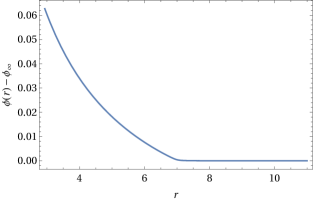
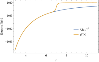
Figure 1: Numerical solutions of Eq. (17) for $H(x)=x$, $Y(r)$ given by Eq. (18) and (19), with boundary data $\phi(r_{\rm max})=1$, $\phi^{\prime}(r_{\rm max})=0$. Here, we use exaggerated parameter choices: $\nu_{0}=1/10$, $Y_{0}=-0.5122$, $r_{0}=7$, $\lambda_{0}=1/8$, and $m_{R}=2.450$. The parameters have been adjusted so that the resulting BH mass parameter is $M_{\rm BH}=1$. The charge parameter is $Q_{\rm BH}=0.3159$ and the ADM mass is $M_{\rm ADM}=2$. The plot on the left is the electric potential $\phi(r)$, and the plot on the right is the electric field $\phi^{\prime}(r)$, and the unshielded electric field profile $-Q_{\rm BH}/r^{2}$.

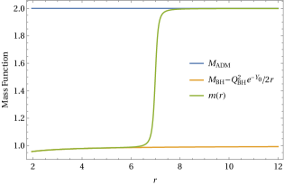
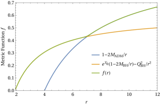
Figure 2: Numerical solutions of Eqs. (21) and (22) corresponding to the electric potential solution of Fig. 1, with BH charge parameter $Q_{\rm BH}=0.3159$, mass parameter $M_{\rm BH}=1$, and the ADM mass $M_{\rm ADM}=6$. On the left is $m(r)$, plotted against the value of $m(\infty)$ and unshielded mass function $(M_{\rm BH}-{Q_{\rm BH}^{2}e^{-Y_{0}}}/{2r})$. On the right is the metric component $f(r)$, plotted against the Schwarzschild value $1-2m(\infty)/r$ and the unshielded Reissner-Nordström metric component given by Eq. (II.2).

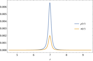
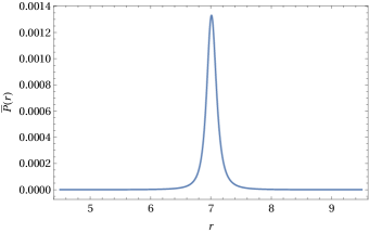
Figure 3: Density and tangential stress profiles corresponding to the solutions in Figs. 1 and 2. On the left are the energy density profile $\rho(r)$ and the charge density profile $n(r)$, which are nearly identical up to a scaling factor. On the right is the tangential stress profile $\bar{P}$; the solution satisfies the dominant energy condition. Qualitatively similar plots can be obtained for other parameter choices.

In this section, we will solve Eq. (13) and show that the screening mechanism arises naturally in a limit for a rather large class of physically motivated charge density profiles. As mentioned in the preceding section, one has a system of four equations for six variables—two supplementary equations are required. Here, we supply these conditions by choosing $Y^{\prime}(r)$ and a relation between the charge density $qn(r)$ and the electrostatic potential $\phi(r)$, motivated by the Debye shielding model in plasma physics.

In the Debye shielding model Chen (2012); Bittencourt (2013), one assumes that the number densities for each particle species satisfies a Maxwell-Boltzmann distribution in the particle energies, and upon integrating out the particle momenta, one finds that the distribution is a function of the electrostatic potential. In the high-temperature limit, one recovers a charge density proportional to the electrostatic potential. In curved spacetime, one should note that since the charge density is defined with respect to the fluid four-velocity, the electrostatic potential in the comoving frame has the form $A_{\mu}u^{\mu}=\phi/\sqrt{f}$ (the rhs being the expression in spherical symmetry). If we also require that the charge density is a fraction of the matter density $\rho(r)$, one arrives at the expression:

$$qn(r)\approx\nu_{0}\frac{\phi(r)\rho(r)}{\sqrt{f(r)}},$$ (15)

which one may regard as the leading order term in the high $kT$ expansion of the general expression:

$$qn(r)=\frac{\nu_{0}kT}{\bar{q}}\frac{\rho(r)}{\sqrt{f(r)}}H(\bar{q}\phi(r)/kT)~{},$$ (16)

where $H(\cdot)$ is a suitably chosen distribution function of the energies of the individual charged particles and $\bar{q}$ is some arbitrary test charge. One might, following the Debye shielding model, construct $H(\cdot)$ from the Maxwell-Boltzmann distribution, so that $H(x)=\exp(x)-1$, but Eq. (16) should apply for any distribution function that reduces to a homogeneous linear function in the high temperature limit for an appropriate rescaling of $\nu_{0}$. With Eqs. (16) and (8), Eq. (13) has the general form:

$$\phi^{\prime\prime}(r)+\frac{2\phi^{\prime}(r)}{r}=\frac{1}{2}Y^{\prime}(r)\left[\frac{\nu_{0}kTqH(\bar{q}\phi(r)/kT)}{\bar{q}r}+\phi^{\prime}(r)\right]$$ (17)

so that, for a choice of distribution function $H(\cdot)$, one can solve for $\phi(r)$, given a function $Y(r)$.

One can motivate choices for $Y(r)$ from Eqs. (8) and (12), and the condition that outside the event horizon, $Y(r)$ is a monotonic function. As a consequence, the most general spherically symmetric solution to the Einstein-Maxwell system in the absence of local charge and energy density is given by Eq. (II.2). Now the system we consider is a charged BH surrounded by charged matter fields with compact support; if we assume a (electro)vacuum near the horizon and at large $r$, then the function $Y(r)$ is a constant near the horizon and at large $r$, but these constant values $Y_{0}$ and $Y_{\infty}=0$ will be different, with $Y_{0}<Y_{\infty}=0$. Therefore, it follows that $\Delta Y_{0}=Y_{0}<0$ near the horizon. These considerations suggest that $Y(r)$ has a step function profile:

$$Y(r)=Y_{0}\,\sigma\left(\frac{r-r_{0}}{\lambda_{0}}\right)~{},$$ (18)

where, $\sigma(x)=0$ for $x\gg 1$ and $\sigma(x)=-1$ for $x\ll-1$. A particularly simple choice, which we employ in our numerical solutions, is the following:

$$\sigma(x)=\frac{1}{2}\left[\frac{x}{\sqrt{x^{2}+1}}-1\right]~{}.$$ (19)

We obtain numerical solutions for (17) with $H(x)=x$ [to recover Eq. (15) in appropriate limit)] with the choice of $Y$ in Eqs. (18) and (19), and for some choice of the constant $Y_{0}$. We integrate Eq. (17) inward from an initial point $r_{\rm max}\gg r_{+}$, with initial data $\phi(r_{\rm max})=\phi_{0}\neq 0$, $\phi^{\prime}(r_{\rm max})=0$. As illustrated in Figs. 1 and 4, the result is consistent with what one might expect; for $r\ll r_{0}$, the potential has the form $\phi(r)=\phi_{0}+Q_{\rm BH}/{r}$, and for $r\gg r_{0}$ $\phi(r)=\phi_{0}$. The BH charge $Q_{\rm BH}$ is obtained by fitting the portion of the solution near the horizon to $\phi^{\prime}(r)=-Q_{\rm BH}/{r^{2}}$. The BH mass, on the other hand, is not fixed by the solution, but one can specify the mass to charge ratio by way of the dimensionless parameter $m_{R}$:

$$\frac{M_{\rm BH}}{Q_{\rm BH}}=m_{R}e^{-Y_{0}/2}~{},$$ (20)

where, we require $m_{R}\geq 1$, with equality corresponding to the extremal limit, also see Eq. (II.2). Given this form for $Y(r)$ and the potential $\phi(r)$ solved from Eq. (17), both the mass function $m(r)$ and the metric component $f(r)$ can be derived. First of all, one solves the following equation using the solution for $\phi(r)$:

$$2m^{\prime}(r)=[r-2m(r)]Y^{\prime}(r)+r^{2}e^{-Y(r)}\phi^{\prime}(r)^{2}~{},$$ (21)

and then using the solution for the mass function from the above equation, to solve

$$\frac{f^{\prime}(r)}{f(r)}=\frac{2m(r)-2rm^{\prime}(r)}{r^{2}-2rm(r)}+Y^{\prime}(r)~{}.$$ (22)

We would like to emphasize that both Eqs. (21) and (22) are a straightforward rewriting of Eqs. (9) and (8), respectively. The solutions of the above differential equations are illustrated in Figs. 2 and 5. The corresponding energy density, charge density, and tangential pressure for an exaggerated parameter choice is displayed in Fig. 3. We choose the parameters so that the energy density vanishes roughly below the Innermost Stable Circular Orbit (ISCO) for uncharged particles surrounding a slightly charged BH.

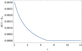
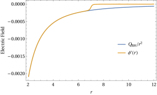
Figure 4: Numerical solutions of Eq. (17) for $H(x)=x$, $Y(r)$ given by Eq. (18) and (19), with boundary data $\phi(r_{\rm max})=1$, $\phi^{\prime}(r_{\rm max})=0$. Here, we use realistic parameter choices: $\nu_{0}=1/50$, $Y_{0}=-0.1276$, $r_{0}=7$, $\lambda_{0}=0.125$, and $m_{R}=108.2$. The parameters have been adjusted so that the resulting BH mass parameter is $M_{\rm BH}=1$. The BH charge parameter is $Q_{\rm BH}=8.667\times 10^{-3}$ and the ADM mass is $M_{\rm ADM}=1.3$. The plot on the left is the electric potential $\phi(r)$, and the plot on the right is the electric field $\phi^{\prime}(r)$ (in yellow), and the unshielded electric field profile $-Q_{\rm BH}/r^{2}$ (in blue).

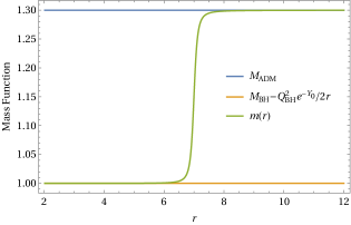
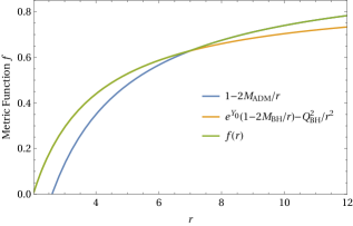
Figure 5: Numerical solutions of Eqs. (21) and (22) corresponding to the electric potential solution of Fig. 4, with BH charge parameter $Q_{\rm BH}=8.667\times 10^{-3}$, mass parameter $M_{\rm BH}=1$, and the ADM mass $M_{\rm ADM}=1.3$. On the left is $m(r)$ (in green), plotted against the value of $m(\infty)$ (in blue) and unshielded mass function $(M_{\rm BH}-{Q_{\rm BH}^{2}e^{-Y_{0}}}/{2r})$ (in yellow). On the right is the metric component $f(r)$ (in green), plotted against the Schwarzschild value $1-2m(\infty)/r$ (in blue) and the unshielded Reissner-Nordström metric component given by Eq. (II.2) (in yellow).

IV Black hole parametrization

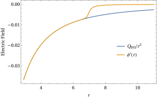
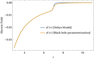
Figure 6: Electric field solution obtained with the BH parametrization for exaggerated parameter choices. Here, we choose $\tilde{Q}_{BH}=0.4081$, $M_{BH}=1$, $M_{ADM}=2$, $r_{0}=7$, $\lambda_{0}=1/8$, and $\delta r_{*0}=-0.1$. The parameters have been chosen so that $M_{BH}$, $Q_{BH}$ and $M_{ADM}$ match that of the Debye model solution in Fig. 1. The parameter $\delta r_{*0}$ has been set so that the charge density is closer to the BH, as one might expect. The solution for the electric field is on the left, and a comparison with the Debye model solution is provided on the right.

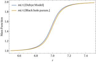
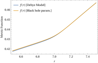
Figure 7: Comparison of geometries between the Debye model and BH parametrization solutions for exaggerated parameter choices in Figs. 1 and 6. The mass function $m(r)$ is on the left, and the metric function $f(r)$ is on the right. The differences in the metric function $f(r)$ for $r<r_{0}=7$ can be attributed to the fact that the value for $Y_{0}=Y(r_{H})=-0.5112$ here differs slightly from the value of $Y_{0}$ for the Debye model solution.

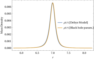
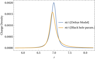
Figure 8: Comparison of density profiles between the Debye model and BH parametrization solutions for exaggerated parameter choices in Figs. 1 and 6. The energy density $\rho(r)$ is on the left, and the charge density $n(r)$ is on the right. We recall the choice $\delta r_{*0}=-0.1$, which shifts the peak of the charge density profile $n(r)$ to a slightly lower radius; we do this because if $\delta r_{*0}$ is chosen to vanish, the BH parametrization tends to shift the peak of $n(r)$ to larger values of $r$ compared to the Debye model. The comparison plot for the tangential pressure profile is qualitatively similar to that of $n(r)$, so we omit it here.

One difficulty with the approach in the preceding section is that in assuming a relationship between the density $n(r)$ and the potential $\phi(r)$, the charge density $n(r)$ is formally sensitive to shifts in the potential $\phi(r)$, though as we have argued, one can in principle absorb such shifts into the parameter $\nu_{0}$ for a Maxwell-Boltzmann-like distribution. In this section, we consider an alternative approach which does not assume a particular relationship between the density $n(r)$ and the potential $\phi(r)$. Instead we perform a physically motivated reparametrization, and choose explicit forms for a pair of functions — such an approach provides a direct phenomenological model for a shielded BH.

We begin by reparameterizing the geometry, in order to bring out the physics of these solutions. First of all, we choose the mass function $m(r)$, as follows:

$$m(r)=M_{\rm BH}-\frac{Q_{\rm BH}^{2}}{2r}e^{-Y_{0}}+\left[\mathcal{M}(r)+\mathcal{Q}(r)\right]e^{-2Y_{0}}f_{\rm EV}^{2}~{},$$ (23)

and the energy density of the fluid as

$$\rho(r)= \frac{2}{8\pi r^{2}}\dfrac{d}{dr}\left[e^{-2Y_{0}}\mathcal{M}(r)f_{\rm EV}^{2}\right]$$ (24)

$$= \frac{2f_{\rm EV}}{e^{2Y_{0}}8\pi r^{2}}\biggl{[}\mathcal{M}^{\prime}(r)f_{\rm EV}+4\mathcal{M}(r)\left(\frac{M_{\rm BH}e^{Y_{0}}}{r^{2}}-\frac{Q_{\rm BH}^{2}}{r^{3}}\right)\biggr{]},$$

where we have introduced the radial function $f_{\rm EV}$ from Eq. (II.2). Thus, we impose that the external mass distribution is such that the geometry contains a central charged Reissner-Nordström-like BH, with mass $M_{\rm BH}$ and charge $\pm Q_{\rm BH}e^{-Y_{0}/2}$. In vacuum, $\mathcal{Q}(r)=\mathcal{M}(r)=0$ and one recovers identically the geometry of Reissner-Nordström BH, since in that case $Y_{0}$ vanishes as well.

Therefore, the $g^{rr}$ component of the metric reads

$$g^{rr}=\frac{f_{\rm EV}}{e^{Y_{0}}}\left[1-\frac{2\mathcal{M}(r)+2\mathcal{Q}(r)}{e^{Y_{0}}r}f_{\rm EV}\right]~{}.$$ (25)

Finally, from Eq. (12), it follows that the function $f(r)$, i.e., the $g_{tt}$ component of the metric, becomes

$$f(r)= \frac{f_{\rm EV}e^{Y(r)}}{e^{Y_{0}}}\left[1-\frac{2\mathcal{M}(r)+2\mathcal{Q}(r)}{e^{Y_{0}}r}f_{\rm EV}\right],$$ (26)

where, the function $Y(r)$ satisfies the following first order differential equation

$$\frac{dY}{dr} =\frac{8\pi r\rho(r)}{g^{rr}}=\frac{2\dfrac{d}{dr}\left[\mathcal{M}(r)f_{\rm EV}^{2}\right]}{f_{\rm EV}\Big{[}e^{Y_{0}}r-\left\{2\mathcal{M}(r)+2\mathcal{Q}(r)\right\}f_{\rm EV}\Big{]}}$$ (27)

$$=\frac{2r^{3}f_{\rm EV}\mathcal{M}^{\prime}(r)-8\mathcal{M}(r)\left(Q_{\rm BH}^{2}-e^{Y_{0}}rM_{\rm BH}\right)}{e^{Y_{0}}r^{4}-2(\mathcal{M}(r)+\mathcal{Q}(r))r^{3}f_{\rm EV}}$$

Note that $(dY/dr)$ and hence $Y(r)$ are both finite in the limit, $r\rightarrow r_{\pm}$, where $r_{\pm}$ are the solutions of the algebraic equation, $f_{\rm RN}=0$. In particular, note that the surfaces $r=r_{\pm}$ are null, since $g^{rr}$ vanishes there and so does $(\partial/\partial t)^{\mu}(\partial/\partial t)_{\mu}$. Therefore, the spacetime has an event horizon at $r=r_{+}=M_{\rm BH}+\sqrt{M_{\rm BH}^{2}-Q_{\rm BH}^{2}e^{-Y_{0}}}$ and a Cauchy horizon at $r=r_{-}=M_{\rm BH}-\sqrt{M_{\rm BH}^{2}-Q_{\rm BH}^{2}e^{-Y_{0}}}$. These are precisely where the horizons of the Reissner-Nordström BHs are located, in this “areal” coordinate. Moreover, as evident from Eq. (24), on the event horizon the energy density $\rho$ identically vanishes, which is also a desirable property. Therefore, we have traded the mass function $m(r)$ and the energy density $\rho(r)$ of the charged cloud in terms of the functions $\mathcal{M}(r)$ and $\mathcal{Q}(r)$. Note that, $Y(r)$ gets determined in terms of these two functions and hence the metric element $g_{tt}$. Therefore, the three unknowns $\{Y(r),m(r),\rho(r)\}$ reduce to the following two unknowns $\{\mathcal{M}(r),\mathcal{Q}(r)\}$.

On a different note, notice that $Y(r)$ satisfies a first order differential equation whose integration needs to be done with the boundary condition that $Y(r\rightarrow\infty)=Y_{\infty}$, which can be chosen to be zero. However, due to the monotonicity of $Y^{\prime}(r)$, it follows that $Y(r_{+})<Y_{\infty}$ and hence $f(r)\neq g^{rr}$ on the horizon, but will differ by an overall factor $\sim e^{Y_{+}-Y_{\infty}}$.

Let us now concentrate on the equations governing the electric potential. First of all, the field equation presented in Eq. (9) needs to be consistent with Eq. (23) and Eq. (24), which fixes the function $\psi(r)$ to be

$$\psi(r) =\frac{2m^{\prime}-8\pi r^{2}\rho}{8\pi r^{2}}$$ (28)

$$=\frac{Q_{\rm BH}^{2}}{8\pi e^{Y_{0}}r^{4}}+\frac{2}{8\pi e^{2Y_{0}}r^{2}}\frac{d}{dr}\left[\mathcal{Q}(r)f_{\rm EV}^{2}\right]~{}.$$

Using Eq. (11), we can express the electric potential as

$$\phi^{\prime}(r)^{2}=\frac{e^{Y(r)}}{e^{2Y_{0}}}\left[\frac{Q_{\rm BH}^{2}e^{Y_{0}}}{r^{4}}+\frac{2}{r^{2}}\frac{d}{dr}\left[\mathcal{Q}(r)f_{\rm EV}^{2}\right]\right]~{}.$$ (29)

We should point out that, as expected, the electric potential depends on the charge of the BH, $Q_{\rm BH}$, and the energy density from the electric field energy of the charged cloud, denoted by $\mathcal{Q}(r)$. In absence of both the electric potential would vanish, as expected.

Finally, from Eq. (13) the differential equation for the electric potential $\phi(r)$ reads

$$\phi^{\prime\prime}+\frac{2\phi^{\prime}}{r} =\frac{\phi^{\prime}}{re^{2Y_{0}}g^{rr}}\dfrac{d}{dr}\left[\mathcal{M}(r)f_{\rm EV}^{2}\right]+\frac{4\pi q\sqrt{f}n(r)}{g^{rr}}$$ (30)

$$=\frac{\phi^{\prime}}{re^{2Y_{0}}g^{rr}}\dfrac{d}{dr}\left[\mathcal{M}(r)f_{\rm EV}^{2}\right]+\frac{4\pi qn(r)}{\sqrt{g^{rr}}}e^{Y(r)/2}~{}.$$

Using Eq. (27), we can rewrite the above equation as

$$\phi^{\prime\prime}+\frac{2\phi^{\prime}}{r} =\frac{\phi^{\prime}Y^{\prime}}{2}+\frac{4\pi qn(r)}{\sqrt{g^{rr}}}e^{Y(r)/2}~{}.$$ (31)

With the reparametrization in hand, one can solve the system of equations by specifying the mass distribution $\mathcal{M}(r)$ and the charge distribution $\mathcal{Q}(r)$, based on their expected forms in regions where the density $\rho(r)$ vanishes. Here, one assumes that the density profile $\rho(r)$ is centered at a radius $r_{0}>r_{+}$, and has a width of $\sigma_{0}$ [so that $\rho(r)$ vanishes for $|r-r_{0}|>\sigma_{0}$]. Near the horizon, one requires:

$$\mathcal{M}(r\rightarrow r_{+}) =0~{},$$ (32)

$$\mathcal{Q}(r\rightarrow r_{+}) =0~{}.$$

At radii $r\gg r_{0}+\sigma_{0}$ one has $\mathcal{M}(r\gg r_{0}+\sigma_{0})\approx\mathcal{M}_{L}(r)$, where

$$\mathcal{M}_{L}(r) :=\frac{r^{4}\left(M_{\rm ADM}-M_{\rm BH}-\mathcal{Q}_{\infty}\right)}{\left(r\left(r-2M_{\rm BH}\right)+\tilde{Q}_{\rm BH}^{2}\right)^{2}}~{},$$ (33)

which can be obtained by solving Eq. (37) when $Y(r)=Y^{\prime}(r)=0$; we define an effective charge $\tilde{Q}_{\rm BH}^{2}:=Q_{\rm BH}^{2}e^{-Y_{0}}$, and the quantity $\mathcal{Q}_{\infty}$ is an integration constant which coincides with the value of $\mathcal{Q}(r)$ at large $r$. The latter can be inferred by solving Eq. (29) for $\mathcal{Q}(r)$ [assuming $\phi^{\prime}(r\gg r_{0}+\sigma_{0})=0$] and solving Eq. (36) for $\mathcal{M}(r)$. One may then write:

$$\mathcal{M}(r)= \sigma_{M}\left(\frac{r_{*}-r_{*0}}{\sigma_{*0}}\right)\mathcal{M}_{L}(r)~{},$$ (34)

where $\sigma_{M}(x)$ is a sigmoidal function, with the property that $\sigma_{M}(-\infty)=0$ and $\sigma_{M}(+\infty)=1$. Here $r_{*}$ is a tortoise coordinate defined with respect to the horizon radius of $f_{\rm EV}$, such that $r_{*}(r)=r+r_{H}\ln(r/r_{H}-1)$ and $r_{*0}=r_{*}(r_{0})$. We define $\sigma_{*0}:=\sigma_{0}r^{\prime}_{*}(r_{0})$, assuming $\sigma_{0}\ll r_{0}$. Given a solution to Eq. (29) for $r\gg r_{0}+\sigma_{0}$, one can assume a similar expression for $\mathcal{Q}(r)$, but it is perhaps more appropriate to specify the derivative of $\mathcal{Q}(r)$ in the following manner:

$$e^{-2Y_{0}}\frac{d}{dr}\left[\mathcal{Q}(r)f_{\rm EV}^{2}\right]=-\sigma_{Q}\left(\frac{r_{*}-r_{*0}-\delta r_{*0}}{\sigma_{*0}}\right)\frac{\tilde{Q}_{\rm BH}^{2}}{2r^{2}},$$ (35)

so that, upon comparison with Eq. (29) and setting $\delta r_{*0}=0$, one has $|\phi^{\prime}(r<r_{0}-\sigma_{0})|\approx|Q_{BH}|/r^{2}$ and $\phi^{\prime}(r>r_{0}+\sigma_{0})\approx 0$. The adjustable parameter $\delta r_{*0}$ has been introduced so that one has control over the position of the charge distribution.

Given the mass distribution $\mathcal{M}(r)$ and the charge distribution $\mathcal{Q}(r)$, one can then solve for $Y(r)$ from Eq. (27), then $\phi^{\prime}(r)$ from Eq. (29), the number density $n(r)$ from Eq. (31) and finally the tangential pressure $\bar{P}$ from Eq. (10). Plots for $\phi^{\prime}(r)$ and the metric functions $m(r)$ and $f(r)$ are provided in the respective Figs. 6 and 7, and the density profile comparisons are provided in Fig. 8.

To compare the results obtained with the present parametrization with that obtained by the method in Sec. III, we note that the following equations hold true:

$$\left[\mathcal{M}(r)+\mathcal{Q}(r)\right]\frac{f_{\rm EV}^{2}}{e^{2Y_{0}}}=m(r)+\frac{Q_{\rm BH}^{2}}{2e^{Y_{0}}r}-M_{\rm BH}~{},$$ (36)

$$\dfrac{d}{dr}\left[e^{-2Y_{0}}f_{\rm EV}^{2}\,\mathcal{M}(r)\right]=\frac{r}{2}f(r)e^{Y(r)}Y^{\prime}(r)~{},$$ (37)

which one may solve for $\mathcal{M}(r)$ and $\mathcal{Q}(r)$, given $m(r)$, $f(r)$, and $Y(r)$. Specifically, one solves Eq. (37) for the mass parameter $\mathcal{M}(r)$ and then Eq. (36) provides the charge function $\mathcal{Q}(r)$. Alternatively, if one has $\phi(r)$ and $Y(r)$ in hand, one can first solve Eq. (29) to obtain $\mathcal{Q}(r)$, then Eq. (36) provides the mass function $\mathcal{M}(r)$. We illustrate in Fig. 9 profiles for $\mathcal{M}(r)$ and $\mathcal{Q}(r)$ obtained from the Debye model solution of Fig. 1.

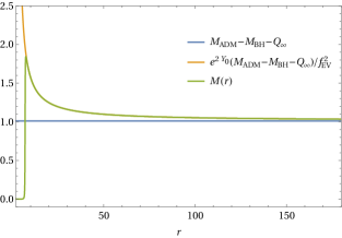
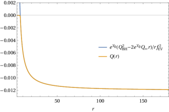
Figure 9: Plots of the functions $\mathcal{M}(r)$ and $\mathcal{Q}(r)$ obtained from the Debye model solutions in Figs. 1 and 2. The profile for $\mathcal{M}(r)$ is the on the left, and the profile for $\mathcal{Q}(r)$ is on the right. The corresponding profiles for the BH parametrization are not shown here, as they are nearly indistinguishable from the plots shown, and are qualitatively similar near $r=r_{0}$.

V Physical Properties of the spacetime

Having derived the metric elements of a charged BH in a charged cloud distribution, within a static and spherically symmetric context, in a closed form, let us note down a few of its interesting physical properties. These will include the location of the photon sphere Claudel et al. (2001), the location of the innermost stable circular orbits, the angular frequency and the Lyapunov exponents associated with the photon sphere. As we have already noted there will be an event horizon, located at $r_{+}=M_{\rm BH}+\sqrt{M_{\rm BH}^{2}-Q_{\rm BH}^{2}e^{-Y_{0}}}$, on which the energy density $\rho$ identically vanishes, while the tangential pressure $\bar{P}$ remains finite.

The photon sphere, or, the unstable circular photon orbits are given by the condition, $rf^{\prime}=2f$, which from Eq. (8) and Eq. (12) yields

$$\frac{8\pi r^{2}\rho}{r-2m(r)} =\frac{rf^{\prime}+f}{rf}-\frac{1-2m(r)^{\prime}}{r-2m(r)}$$ (38)

$$=\frac{3}{r}-\frac{1-2m(r)^{\prime}}{r-2m(r)}~{}.$$

Using Eq. (9), we can express the above equation as

$$\frac{8\pi r^{2}\rho}{r-2m(r)}=\frac{2}{r}\left(\frac{r-3m(r)}{r-2m(r)}\right)+\frac{8\pi r^{2}\rho+8\pi r^{2}\psi}{r-2m}~{},$$ (39)

yielding the following expression satisfied by the radius of the photon sphere:

$$r =3m(r)-\frac{8\pi r^{3}\psi}{2}$$ (40)

$$=3M_{\rm BH}-\frac{2Q_{\rm BH}^{2}}{e^{Y_{0}}r}+3\frac{f_{\rm EV}^{2}}{e^{2Y_{0}}}\left[\mathcal{M}(r)+\mathcal{Q}(r)\right]$$

$$\qquad\qquad-\frac{r}{e^{2Y_{0}}}\frac{d}{dr}\left[\mathcal{Q}(r)f_{\rm EV}^{2}\right]~{}.$$

Note that, in the absence of any charge on the BH, as well as the absence of charged cloud leads to the well known radius of the photon sphere, at $r_{\rm ph}=3M_{\rm BH}$. However, presence of a charged matter distribution and charge on the BH itself shifts the photon circular orbit to a different value. In the case where $\mathcal{M}(r)=\mathcal{Q}(r)=0$, one has a photon sphere radius:

$$r_{\rm ph,EV} =\frac{1}{2}\left(3M_{\rm BH}+\sqrt{9M_{\rm BH}^{2}-8e^{-Y_{0}}Q_{\rm BH}^{2}}\right),$$ (41)

which differs from the usual Reissner-Nordström result due to the presence of the factor $e^{-Y_{0}}$. Also the critical impact parameter $b_{\rm crit}\equiv(L_{\rm crit}/E_{\rm crit})$, related to the capturing of null geodesics by the BH with the charged cloud system, would correspond to $E_{\rm crit}=V_{\rm max}$, where $V_{\rm max}$ corresponds to the maximum of the effective potential. For photons, the maxima corresponds to the photon sphere, and, hence,

$$b_{\rm crit}=\frac{r_{\rm ph}}{\sqrt{f(r_{\rm ph})}}=\frac{r_{\rm ph}^{3/2}}{\sqrt{r_{\rm ph}-2m(r_{\rm ph})}}~{}e^{-Y(r_{\rm ph})/2}~{},$$ (42)

where $r_{\rm ph}$ corresponds to the location of the photon sphere, which is a solution to Eq. (40). The angular frequency and the Lyapunov exponent associated with the photon sphere reads

$$\Omega_{\rm ph} =\frac{1}{b_{\rm crit}}~{};$$ (43)

$$\lambda_{\rm ph} =\sqrt{\left(1-\frac{2m(r_{\rm ph})}{r_{\rm ph}}\right)\left(\frac{2f(r_{\rm ph})-r_{\rm ph}^{2}f^{\prime\prime}(r_{\rm ph})}{2r_{\rm ph}^{2}}\right)}~{}.$$ (44)

These provide the basic properties of the photon sphere. In particular, the angular frequency $\Omega_{\rm ph}$ and Lyapunov exponent $\lambda_{\rm ph}$ are respectively related to the real and imaginary parts of the quasinormal mode frequencies in the eikonal limit ($n$ and $l$ being nonnegative integers):

$$\omega_{\rm ps} =l\Omega_{\rm ph}-i(n+1/2)|\lambda_{\rm ph}|,\ \qquad l\gg 1.$$ (45)

Therefore, the above expressions enable us to compute the quasinormal modes of the charged cloud surrounding a charged BH system, in the large angular momentum limit. So far, all the results we have derived are analytic in nature. However, for obtaining a solution to the electrostatic potential, as well as to the tangential pressure and the metric elements, we need solutions for the differential equations presented in the previous section. This in turn will enable us to derive the location of the photon sphere from Eq. (40) and hence its related properties.

Values for the photon sphere radii $r_{\rm ph}$ and values for the quantities characterizing null geodesics near $r_{\rm ph}$ for the numerical solutions described in the preceding sections are given in Table 1. We note that since the energy density becomes sparse in the vicinity of the photon sphere (as we have chosen the energy density to vanish below the ISCO), the photon sphere mode frequencies for quasinormal modes in the Eikonal limit are equivalent to those of an electrovacuum Reissner-Nordström BH with a rescaled time coordinate. However, since $e^{Y_{0}}\neq 1$ below the cloud, the quasinormal mode frequencies as seen by an observer at infinity will differ between that of a “naked” charged BH, and one that is “clothed” by a plasma.

Properties of null geodesics near photon sphere
	$r_{\rm ph}$	$b_{\rm crit}$	$\Omega_{\rm ph}$	$\lambda_{\rm ph}$
Realistic values	$2.99994$	$5.53852$	$0.180554$	$0.180552$
Exaggerated values	$2.88411$	$6.51911$	$0.153395$	$0.150292$
Realistic RN	$2.99995$	$5.19608$	$0.192453$	$0.192451$
Exaggerated RN	$2.93153$	$5.10730$	$0.195798$	$0.193511$

Table 1: The row termed “Realistic values” corresponds to the parameter choices of the Debye model solution in Fig. 4. The row termed “Exaggerated values” corresponds to the parameter choices of the Debye model solution in Fig. 1. The rows termed “Realistic RN” and ‘Exaggerated RN” correspond to the same parameter choices for $M_{BH}$ and $Q_{BH}$ as the respective rows “Realistic values” and “Exaggerated values”, except with the Reissner-Nordström value for the factor $e^{Y_{0}}=1$. Regardless of the model, the results are the same (up to precision errors) near the photon sphere radius $r_{\rm ph}$, as the energy density for the cases considered becomes sparse at the photon radius; essentially, $r_{\rm ph}$ is the photon radius obtained from $f_{\rm EV}$.

VI Conclusions

The exact mechanism shielding a charged BH has remained elusive to date. In this work we present a comprehensive understanding of the screening mechanism of spherically symmetric charged BH surrounded by a spherically symmetric charged matter distribution. Since there is no radial outflow, as consistent with the galactic matter distribution, we also consider an anisotropic matter distribution surrounding the BH having only energy density and tangential stress, all functions of the radial coordinate alone. The resulting system has—(a) two metric degrees of freedom, the $g_{tt}$ and $g^{rr}$ components, (b) the energy density and tangential pressure of the matter distribution, (c) the electrostatic potential and (d) the charge density—in total six functions of the radial coordinate alone. Since the energy and charge densities are independent, our model can may be regarded as a rather general effective description for charge overdensities in plasmas surrounding charged BHs. However, the Einstein equations along with the Maxwell equations provide four equations among these six variables—this is not particularly surprising, as our model might be regarded as an effective description for a multispecies fluid, in which case one must supply equations of state for each fluid species. Thus in order to close this system of equations, we need two more relations among these variables. For that we make two possible choices—(a) we provide a relation between the number density of the charged particles with the electrostatics potential along with a suitable choice for the ratio of the $g_{tt}$ and $g^{rr}$ components of the metric, alternatively, (b) we fix the mass function $\mathcal{M}(r)$ and the charge function $\mathcal{Q}(r)$ in the parametrized form of the geometry, describing the charged matter, surrounding the charged BH. Both of these approaches results in an electric field decaying sufficiently rapidly; see, e.g., Fig. 6. In particular, fixing the relation between the number density of charged particles with the electrostatic potential to be linear, results in a much faster exponential decay, than a steep power law decay in the parametrized case. Nonetheless, for generic choices of parameters, the screening effect of the electric field remains, such that after moving a small distance into the charged cloud, the electric field almost diminishes to zero and hence it appears that overall the system is uncharged, though there is a charged BH inside.

This mechanism is intuitive, but has never been derived in an explicit manner. Here, we directly solve the full nonlinear Einstein-Maxwell system, by two independent methods as prescribed above: in doing so, we obtain a description that accounts for the nonlinearities of general relativity. In both of these cases, such a screening mechanism appears generically, providing a direct proof that indeed the electric field of a charged BH almost vanishes immediately after the internal surface of the charged cloud is crossed. Since, in most of the astrophysical scenario the BHs are surrounded by charged plasma, it follows that astrophysically, i.e., from a large distance from the central BH, it will always appear to be neutral. This is why astrophysical BHs appears to be uncharged, due to the screening mechanism derived here.

The matter distributions we have considered in this analysis are assumed to vanish for radii below the innermost stable circular orbit for uncharged particles. Consequently, the physical properties of null geodesics near the photon sphere are essentially those of a charged BH in electrovacuum, but we have found that the presence of the plasma cloud changes the redshift factor, so that the eikonal limit quasinormal modes seen by a faraway observer will differ from an “unclothed” charged BH. Still, we have presented general formulas for the angular frequency and Lyapunov exponent in case one wishes to extend the analysis to charged Einstein cluster models incorporating unstable circular orbits near the photon sphere.

There are several future applications of the results discussed above. The most immediate one would be generalization to Kerr-Newman BHs and show that the screening mechanism continues to hold in the presence of rotation as well. This is important, since all the astrophysical BHs are supposed to have nonzero rotation. It would be interesting to observe effects of the BH charge on the gravitational waves emanating from perturbation of the same as it propagates through the surrounding charged matter. In particular, whether the screening effect will also affect the gravitational wave needs to be explored. It would also be worthwhile to explore if similar results hold true for charges induced by gravitational interactions as well, e.g., what happens to scalar hairs, or hairs inherited from higher spacetime dimensions. These issues will be addressed elsewhere.