Deep Learning for Time Series Anomaly Detection: A Survey

Abstract.

Time series anomaly detection is important for a wide range of research fields and applications, including manufacturing and healthcare. The presence of anomalies can indicate novel or unexpected events, such as production faults, system defects, heart palpitations, and is therefore of particular interest. The large size and complex patterns in time series data have led researchers to develop specialised deep learning models for detecting anomalous patterns. This survey provides a structured and comprehensive overview of the state-of-the-art in deep learning for time series anomaly detection. It provides a taxonomy based on anomaly detection strategies and deep learning models. Aside from describing the basic anomaly detection techniques in each category, their advantages and limitations are also discussed. Furthermore, this study includes examples of deep anomaly detection in time series across various application domains in recent years. Finally, it summarises open issues in research and challenges faced while adopting deep anomaly detection models to time series data.

1. Introduction

The detection of anomalies, also known as outlier or novelty detection, has been an active research field in numerous application domains since the 60s (Grubbs, 1969). As computational processes evolve, the collection of big data and its use in artificial intelligence (AI) is better enabled, contributing to time series analysis including the detection of anomalies. With greater data availability, and increasing algorithmic efficiency/computational power, time series analysis is increasingly being used to address business applications through forecasting, classification, and anomaly detection (Esling and Agon, 2012), (Carreño et al., 2020). There is a growing demand for time series anomaly detection in a wide variety of domains including urban management, intrusion detection, medical risk, and natural disasters, thereby raising its importance.

As deep learning has advanced significantly over the past few years, it has become increasingly capable of learning expressive representations of complex time series, like multidimensional data with both spatial (intermetric) and temporal characteristics. In deep anomaly detection, neural networks are used to learn feature representations or anomaly scores in order to detect anomalies. Many deep anomaly detection models have been developed, providing significantly higher performance than traditional time series anomaly detection tasks in different real-world applications.

Although the field of anomaly detection has been explored in several literature surveys (Chandola et al., 2009), (Pang et al., 2021), (Chalapathy and Chawla, 2019), (Blázquez-García et al., 2021), (Braei and Wagner, 2020) and some evaluation review papers exist (Schmidl et al., 2022), (Kim et al., 2022), there is only one survey on deep anomaly detection methods for time series data (Choi et al., 2021). However, this survey has not covered the vast range of time series anomaly detection methods that have emerged in the recent years such as DAEMON (Chen et al., 2021b), TranAD (Tuli et al., 2022), DCT-GAN (Li et al., 2021a), and Interfusion (Li et al., 2021b). As a result, there is a need for a survey that enables researchers identify the important future directions of research in time series anomaly detection and the methods that are suitable to various application settings. Specifically, this article makes the following contributions:

• A novel taxonomy of time series deep anomaly detection models is presented. Generally, deep time series anomaly detection models are classified into three categories, corresponding to forecasting-based, reconstruction-based, and hybrid methods. Each category is further divided into subcategories, which are defined according to the deep neural network architectures used in the models. Models are characterised by a variety of different structural features which contribute to their detection capabilities.

• This study provides a comprehensive review of the current state of the art. A clear picture can be drawn of the direction and trends in this field.

• The primary benchmarks and datasets that are currently being used in this field are collected, described and hyperlinks are provided.

• A discussion of the fundamental principles that may underlie the occurrence of different anomalies in time series is provided.

The rest of this article is organised as follows: In Section 2, we start with preliminary definition of time series. A taxonomy is then outlined for categorisation of anomalies in time series data. Section 3, discusses how a deep anomaly detection model can be applied to time series data. Different deep models and their capabilities are then presented based on the main approaches (forecasting-based, reconstruction-based, hybrid) and the main architectures of deep neural networks. An overview of publicly available and commonly used datasets for the considered anomaly detection models can be found in Section 4. Additionally, Section 5 explores the applications area of time series deep anomaly detection models in different domains. Finally, Section 6 provides several challenges in this field that can serve as future opportunities.

2. Background

A time series is a series of data points indexed sequentially over time. The most common form of time series is a sequence of observations recorded over time (Hamilton, 2020). Time series are often divided into univariate (one-dimensional) and multivariate (multi-dimensional). These two types are defined in the following subsections. Thereafter, decomposable components of the time series are outlined. Following that, we provide a taxonomy of anomaly types based on time series’ components and characteristics.

2.1. Univariate Time Series

As the name implies, a univariate time series (UTS) is a series of data that is based on a single variable that changes over time, as shown in Fig. 1. Keeping a record of the humidity level every hour of the day would be an example of this. $X$ with $t$ timestamps can be represented as an ordered sequence of data points in the following way:

(1) $$X=(x_{1},\ x_{2},\ldots,\ x_{t})$$

where $x_{i}$ represents the data at timestamp $i\in T$ and $T=\{1,2,...,t\}$.

2.2. Multivariate Time Series

Additionally, a multivariate time series (MTS) represents multiple variables that are dependent on time, each of which is influenced by both past values (stated as ”temporal” dependency) and other variables (dimensions) based on their correlation. The correlations between different variables are referred to as spatial or intermetric dependencies in the literature and they are used interchangeably. In the same example, air pressure and temperature would also be recorded every hour besides humidity level.

An example of a MTS with two dimensions is illustrated in Fig. 2. Consider a multivariate time series represented as a vector $X_{t}$ with $d$ dimensions as follows:

(2) $$X_{t}=(x^{1}_{t},\ x^{2}_{t},\ldots,\ x^{d}_{t})$$

where the $j$th row of $X_{t}$ is $x^{j}_{t}$ that represents the data for timestamp $t$ for the $j$th dimension, and $j=\{1,2,...,d\}$, in which $d$ is the number of dimensions.

2.3. Time series decomposition

It is possible to decompose a time series $X$ into four components that each express a specific aspect of its movement (Dodge, 2008). The components are as follows:

• Secular trend: Data trends occur when there is a long-term upward or downward movement. In fact, the secular trend represents the general pattern of the data over time, and it does not have to be linear. The change in population in a particular region over several years is an example of nonlinear growth or decay depending on various dynamical factors.

• Seasonal variations: Depending on the month, weekday, or duration, a time series may exhibit a seasonal pattern. Seasonality always occurs at a fixed frequency. For instance, a study of gas/electricity consumption shows that the consumption curve does not follow a similar pattern throughout the year. Depending on the season and the locality, the pattern is different.

• Cyclical fluctuations: A cycle is defined as a rise or drop in data without a fixed frequency. Also, it is known as the shape of time series. Cyclic fluctuations can occur in time series due to natural events, such as daily temperature variations.

• Irregular variations: It refers to random, irregular events. It is the residual after all the other components are removed. A disaster such as an earthquake or flood can lead to irregular variations.

A time series is mathematically described by estimating its four components separately, and each of them may deviate from the normal behaviour.

2.4. Anomaly in Time Series

According to (Hawkins, 1980), the term anomaly refers to a deviation from the general distribution of data, such as a single observation (point) or a series of observations (subsequence) that deviate greatly from the general distribution. A very small proportion of the dataset has anomalies, which implies that a dataset is normally distributed. There may be considerable amounts of noise embedded in real-world data, and such noise may be irrelevant to the researcher (Aggarwal, 2017). The most meaningful deviations are usually those that are significantly different from the norm. In circumstances where noise is present, the main characteristics of the data are identical. In data such as time series, trend analysis and anomaly detection are closely related, but they are not equivalent (Aggarwal, 2017). It is possible to see changes in time series datasets owing to concept drift, which occurs when values and trends change over time gradually or abruptly (Masud et al., 2010), (Aggarwal, 2007).

2.4.1. Types of Anomalies

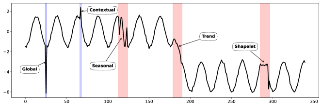
Figure 1. An overview of different temporal anomalies plotted from the NeurIPS-TS dataset (Lai et al., 2021). Global and contextual anomalies occur in a point (coloured in blue), while other types, including seasonal, trend and shapelet, can be occurred in a subsequence (coloured in red).

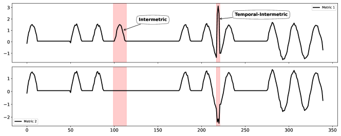
Figure 2. Intermetric and temporal-intermetric anomalies in multivariate time series. In this figure, metric 1 is power consumption, and metric 2 is CPU usage.

Anomalies in UTS and MTS can be classified as temporal, intermetric, or temporal-intermetric anomalies (Li et al., 2021b). In a time series, temporal anomalies can be compared with either their neighbours (local) or the whole time series (global), and they present different forms depending on their behavior (Lai et al., 2021). There are several types of temporal anomalies that commonly occur in univariate time series, all of which are shown in Fig. 1. Temporal anomalies can also occur in the MTS and affect multiple dimensions or all dimensions. A subsequent anomaly may appear when an unusual pattern of behavior emerges over time; however, each observation may not be considered an outlier by itself. As a result of a point anomaly, an unexpected event occurs at one point in time, and it is assumed to be a short sequence. Different types of the temporal anomaly are as follow:

• Global: They are spikes in the series, which are point(s) with extreme values compared to the rest of the series. A global anomaly, for instance, is an unusually large payment by a customer on a typical day. Considering a threshold, it can be described as Eq. (3).

  (3) $$|x_{t}-\hat{x}_{t}|>threshold$$

  where $\hat{x}$ is the output of the model. If the difference between the output and actual point value is greater than a threshold, then it is been recognised as an anomaly. An example of a global anomaly is shown on the left side of Fig. 1 where $-6$ has a large deviation from the time series.

• Contextual: A deviation from a given context would be defined as a deviation from a neighbouring time point, defined here as one that lies within a certain range of proximity. These types of outliers are small glitches in sequential data, which are deviated values from their neighbours. It is possible for a point to be normal in one context while an anomaly in another. For example, large interactions, such as those on boxing day, is considered normal, but not so on other days. The formula is the same as that of a global anomaly, but the threshold for finding anomalies differs. The threshold is determined by taking into account the context of neighbours:

  (4) $$threshold\ \approx\lambda\ *\ var(X_{t-w}:_{t+w})$$

  where $X_{t-w}:_{t+w}$ refers to the context of the data point $x_{t}$ with a window size $w$, $var$ is the variance of the context of data point, and $\lambda$ controlling coefficient for the threshold. The second blue highlight in the Fig. 1 is a contextual anomaly that occurs locally in a specific context.

• Seasonal: In spite of the time series’ similar shapes and trends, their seasonality is unusual compared to the overall seasonality. An example is the number of customers in a restaurant during a week. Such a series has a clear weekly seasonality that makes sense to look for deviations in this seasonality and process the anomalous periods individually.

  (5) $$diss_{s}(S,\ \hat{S})>threshold$$

  where $diss_{s}$ is a function measuring the dissimilarity between two subsequences and $\hat{S}$ denotes the seasonality of the expected subsequences. As demonstrated in the first red highlight of Fig. 1, the seasonal anomaly change the frequency of a rise and drop of data in the particular segment.

• Trend: The event that causes a permanent shift in the data to its mean and produces a transition in the trend of the time series. While this anomaly preserves its cycle and seasonality of normality, it drastically alters its slope. Trends can occasionally change direction, meaning they may go from increasing to decreasing and vice versa. As an example, when a new song comes out, it becomes popular for a while, then it disappears from the charts like the segment in Fig. 1 where the trend changed and is assumed as trend anomaly. It is likely that the trend will restart in the future.

  (6) $$diss_{t}(T,\ \hat{T})>threshold$$

  where $\hat{T}$ is the normal trend.

• Shapelt: There is a subsequence whose shapelet or cycle differs from the normal shapelet component of the sequence. Variations in economic conditions like productivity or the total demand for and supply of the goods and services are often the cause of these fluctuations. In the short-run, these changes lead to periods of expansion and recession.

  (7) $$diss_{c}(C,\ \hat{C})>threshold$$

  where $\hat{C}$ specifies the cycle or shape of expected subsequences. For example, the last highlight in 1 where shape of the segment changed due to some fluctuations.

In this context, the optimal alignment of two time series is used in dynamic time warping (DTW) (Müller, 2007) for determining the dissimilarity between them, thus, DTW has been applied to anomaly detection (Benkabou et al., 2018), (Song et al., 2022). Moreover, MTS is composed of multiple dimensions (a.k.a, metrics) that each describes a different aspect of a complex entity. Spatial dependencies (correlations) among metrics within an entity are also known as intermetric dependencies and can be linear or nonlinear. MTS would exhibit a wide range of anomalous behaviour if these correlations were broken. An example is shown in the left part of Fig. 2, the correlation between power consumption (metric 1) and CPU usage (metric 2) usage is positive, but it breaks about 100th of a second after it begins. Such an anomaly was named the intermetric anomaly in this study.

(8) $$diss_{corr}(corr(X^{j},X^{k}),\ corr(X^{j}_{t:t+w},X^{k}_{t:t+w}))>threshold$$

where $X^{j}$ and $X^{k}$ are two different metrics of MTS that are correlated, and $corr$ measures the correlations between two metrics. When this correlation deteriorates in the window $t:t+w$, it means that the coefficient deviates more than $threshold$ from the normal coefficient.

Intermetric-temporal anomalies are easier to detect from either a temporal or metric perspective since they violate both intermetrics and temporal dependencies, as shown on the right side of Fig. 2.

3. Deep Anomaly Detection Methods

In data with complex structures, deep neural networks are powerful methods for modelling dependencies. A number of scholars have investigated its application to anomaly detection using a variety of deep learning architectures, as illustrated in Fig 3.

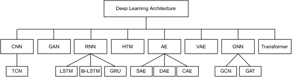
Figure 3. Deep Learning architecture used in time series anomaly detection

3.1. Time Series Anomaly Detection

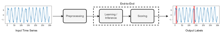
Figure 4. General components of deep anomaly detection models in time series

An overview of deep anomaly detection models in time series is shown in Fig. 4. In our study, deep models for anomaly detection in time series are categorised based on their main approach and architectures. There are two main approaches (learning component in Fig. 4) in the time series anomaly detection literature: forecasting-based and reconstruction-based. A forecasting-based model can be trained to predict the next time stamp, whereas a reconstruction-based model can be deployed to capture the embedding of time series data. A categorisation of deep learning architectures in time series anomaly detection is shown in Fig. 3.

The time series anomaly detection models are summarised in Table 1 and Table 2 based on the input dimensions they process, which are univariate and multivariate time series, respectively. These tables give an overview of the following aspects of the models: 1) Temporal/Spatial, 2) Learning scheme, 3) Input, 4) Interpretability, 5) Point/Sub-sequence anomaly, 6) Stochasticity and 7) Incremental.

3.1.1. Temporal/Spatial

With a univariate time series as input, a model can capture temporal information (i.e, pattern), while with a multivariate time series as input, it can learn normality through both temporal and spatial dependencies. Moreover, if the model input is a multivariate time series in which spatial dependencies are captured, the model can also detect inter-metric anomalies (shown in Fig. 2).

3.1.2. Learning scheme

In practice, training data tends to have a very small number of anomalies that are labelled. As a consequence, most of the models attempt to learn the representation or features of normal data. Based on anomaly definitions, anomalies are then detected by finding deviations from normal data. There are four learning schemes in the recent deep models for anomaly detection: unsupervised, supervised, semi-supervised, and self-supervised. These are based on the availability (or lack) of labelled data points. Supervised method employs a distinct method of learning the boundaries between anomalous and normal data that is based on all the labels in the training set. It can determine an appropriate threshold value that will be used for classifying all timestamps as anomalous if the anomaly score (Section 3.1) assigned to those timestamps exceeds the threshold. The problem with this method is that it is not applicable to applications in the real world because anomalies are often unknown or improperly labelled. In contrast, Unsupervised approach to anomaly detection uses no labels and makes no distinction between training and testing datasets. These techniques are the most flexible since they rely exclusively on intrinsic features of the data. They are useful in streaming applications because they do not require labels for training and testing. Despite these advantages, researchers may encounter difficulties evaluating anomaly detection models using unsupervised methods. The anomaly detection problem is typically treated as an unsupervised learning problem due to the inherently unlabeled nature of historical data and the unpredictable nature of anomalies. In cases where the dataset only consists of normal points, and there are no anomalies, Semi-supervised approaches may be utilised. Afterwards, a model is trained to fit the time series distribution and detects any points that deviate from this distribution as anomalies. Self-supervised methods are trained to predict any of the input’s unobserved parts (or properties) from its observed parts by fully exploiting the unlabeled data itself. This process involves two steps: the first is to determine the parameters of the model based on pseudo-labels, followed by implementing the actual task through supervised or unsupervised learning (e.g., through designing pretext tasks).

3.1.3. Input

A model may take an individual point (i.e., a time step) or a window (i.e., a sequence of time steps containing historical information) as an input. Windows can be used in order, also called sliding windows, or shuffled without regard to the order depending on the application. To overcome the challenges of comparing subsequences rather than points, many models use representations of subsequences (windows) instead of raw data and employ sliding windows that contain the history of previous time steps that rely on the order of subsequences within the time series data. A sliding window extraction is performed in the preprocessing phase after other operations have been implemented, such as imputing missing values, downsampling or upsampling of the data, and data normalisation.

3.1.4. Interpretability

In interpretation, the explanation for why an observation is anomalous is given. Interpretability is essential when anomaly detection is used as a diagnostic tool since it facilitates troubleshooting and analysing anomalies. Multivariate time series are challenging to interpret, and stochastic deep learning complicates the process even further. A typical procedure to troubleshoot entity anomalies involves searching for the top metric that differs most from previously observed behaviour. In light of that, it is, therefore, possible to interpret a detected entity anomaly by analysing several metrics with the highest anomaly scores. Different metrics are used in studies in the absence of standardised metrics for evaluating anomalies’ interpretability. Accordingly, a revised metric called HitRate@P% is defined in (Su et al., 2019) based on the concept of HitRate@K for recommender systems (Yang et al., 2012). In this respect, the Interpretation Score (IPS), adapted from HitRate@K, is outlined to evaluate the anomaly interpretation accuracy at segment level (Li et al., 2021b).

3.1.5. Point/Subsequence anomaly

The model can detect either point anomalies or subsequence anomalies. A point anomaly is a point that is unusual when compared with the rest of the dataset. Subsequence anomalies occur when consecutive observations have unusual cooperative behaviour, although each observation is not necessarily an outlier on its own. Different types of anomalies are described in Section 2.4 and illustrated in Fig. 1 and Fig. 2

3.1.6. Stochasticity

As shown in Tables 1 and 2, we investigate the stochasticity of anomaly detection models as well. Deterministic models can accurately predict future events without relying on randomness. Predicting something that is deterministic is easy because you have all the necessary data at hand. The models will produce the same exact results for a given set of inputs in this circumstance. Stochastic models can handle uncertainties in the inputs. Through the use of a random component as an input, you can account for certain levels of unpredictability or randomness.

3.1.7. Incremental

Incremental learning is a machine learning paradigm in which the model’s knowledge extends whenever one or more new observations appear. It specifies a dynamic learning strategy that can be used if training data becomes available gradually. The goal of incremental learning is to adapt a model to new data while preserving its past knowledge.

Table 1. Univariate Deep Anomaly Detection Models in Time Series

A1	MA1	Model	Su/Un2	Input	P/S3
Forecasting	RNN (3.2.1)	LSTM-AD (Malhotra et al., 2015)	Un	P	Point
		LSTM RNN (Bontemps et al., 2016)	Semi	P	Subseq
		LSTM-based (Ergen and Kozat, 2019)	Un	W	-
		TCQSA (Liu et al., 2020)	Su	P	-
	HTM (3.2.4)	Numenta HTM (Ahmad et al., 2017)	Un	-	-
		Multi HTM (Wu et al., 2018)	Un	-	-
	CNN (3.2.2)	SR-CNN (Ren et al., 2019)	Un	W	Point + Subseq
Reconstruction	VAE (3.3.2)	Donut (Xu et al., 2018)	Un	W	Subseq
		Buzz (Chen et al., 2019)	Un	W	Subseq
		Bagel (Li et al., 2018)	Un	W	Subseq
	AE (3.3.1)	EncDec-AD (Malhotra et al., 2016)	Semi	W	Point

¹ A: Approach, ² Su/Un: Supervised/Unsupervised — Values: [Su: Supervised, Un: Unsupervised, Semi: Semi-supervised, Self: Self-supervised], ³ P/S: Point/Sub-sequence

Table 2. Multivariate Deep Anomaly Detection Models in Time Series

A1	MA2	Model	T/S3	Su/Un4	Input	Int5	P/S6	Stc7	Inc8
Forecasting	RNN (3.2.1)	LSTM-NDT (Hundman et al., 2018)	T	Un	W	✓	Subseq
		DeepLSTM (Chauhan and Vig, 2015)	T	Semi	P		Point
		LSTM-PRED (Goh et al., 2017)	T	Un	W	✓	-
		LGMAD (Ding et al., 2019)	T	Semi	P		Point
		THOC (Shen et al., 2020)	T	Self	W		Subseq
		AD-LTI (Wu et al., 2020)	T	Un	P		Point (frame)
	CNN (3.2.2)	DeepAnt (Munir et al., 2018)	T	Un	W		Point + Subseq
		TCN-ms (He and Zhao, 2019)	T	Semi	W		Subseq
	GNN (3.2.3)	GDN (Deng and Hooi, 2021)	S	Un	W	✓	-
		GTA* (Chen et al., 2021a)	ST	Semi	-		-
		GANF (Dai and Chen, 2022)	ST	Un	W
	HTM (3.2.4)	RADM (Ding et al., 2018)	T	Un	W		-
	Transformer (3.2.5)	SAND (Song et al., 2018)	T	Semi	W		-
		GTA* (Chen et al., 2021a)	ST	Semi	-		-
Reconstruction	AE (3.3.1)	AE/DAE (Sakurada and Yairi, 2014)	T	Semi	P		Point
		DAGMM (Zong et al., 2018)	S	Un	P		Point	✓
		MSCRED (Zhang et al., 2019c)	ST	Un	W	✓	Subseq
		USAD (Audibert et al., 2020)	T	Un	W		Point
		APAE (Goodge et al., 2020)	T	Un	W		-
		RANSynCoders (Abdulaal et al., 2021)	ST	Un	P	✓	Point		✓
		CAE-Ensemble (Campos et al., 2021)	T	Un	W		Subseq
		AMSL (Zhang et al., 2022)	T	Self	W		-
	VAE (3.3.2)	LSTM-VAE (Park et al., 2018)	T	Semi	P		-
		OmniAnomaly (Su et al., 2019)	T	Un	W	✓	Point + Subseq	✓
		STORN (Sölch et al., 2016)	ST	Un	P		Point
		GGM-VAE (Guo et al., 2018)	T	Un	W		Subseq
		SISVAE (Li et al., 2020)	T	Un	W		Point
		VAE-GAN (Niu et al., 2020)	T	Semi	W		Point
		VELC (Zhang et al., 2019b)	T	Un	-		-
		TopoMAD (He et al., 2020)	ST	Un	W		Subseq	✓
		PAD (Chen et al., 2021c)	T	Un	W		Subseq
		InterFusion (Li et al., 2021b)	ST	Un	W	✓	Subseq
		MT-RVAE* (Wang et al., 2022)	ST	Un	W		-
		RDSMM (Li et al., 2022)	T	Un	W		Point + Subseq	✓
	GAN (3.3.3)	MAD-GAN (Li et al., 2019)	ST	Un	W		Subseq
		BeatGAN (Zhou et al., 2019)	T	Un	W		Subseq
		DAEMON (Chen et al., 2021b)	T	Un	W	✓	Subseq
		FGANomaly (Du et al., 2021)	T	Un	W		Point + Subseq
		DCT-GAN* (Li et al., 2021a)	T	Un	W		-
	Transformer (3.3.4)	Anomaly Transformer (Xu et al., 2021)	T	Un	W		Subseq
		TranAD (Tuli et al., 2022)	T	Un	W	✓	Subseq
		DCT-GAN* (Li et al., 2021a)	T	Un	W		-
		MT-RVAE* (Wang et al., 2022)	ST	Un	W		-
Hybrid	AE (3.4.1)	CAE-M (Zhang et al., 2021)	ST	Un	W		Subseq
		NSIBF* (Feng and Tian, 2021)	T	Un	W		Subseq
	RNN (3.4.2)	NSIBF* (Feng and Tian, 2021)	T	Un	W		Subseq
		TAnoGAN (Bashar and Nayak, 2020)	T	Un	W		Subseq
	GNN (3.4.3)	MTAD-GAT (Zhao et al., 2020)	ST	Self	W	✓	Subseq
		FuSAGNet (Han and Woo, 2022)	ST	Semi	W		Subseq

¹ A: Approach, ² MA: Main Architecture, ³ T/S: Temporal/Spatial — Values: [S:Spatial, T:Temporal, ST:Spatio-Temporal], ⁴ Su/Un: Supervised/Unsupervised — Values: [Su: Supervised, Un: Unsupervised, Semi: Semi-supervised, Self: Self-supervised], ⁵ Int: Interpretability, ⁶ P/S: Point/Sub-sequence, ⁷ Stc: Stochastic, ⁸ Inc: Incremental, ^∗ Models with more than one main architecture.

Moreover, the deep model processes the input in a step-by-step or end-to-end fashion (see Fig. 4). In the first category (step-by-step), there is a learning module followed by an anomaly scoring module. It is possible to combine the two modules in the second category to learn anomaly scores using neural networks as an end-to-end process. An output of these models may be anomaly scores or binary labels for inputs. Contrary to algorithms whose objective is to improve representations, DevNet (Pang et al., 2019) for example, introduces deviation networks to detect anomalies by leveraging a few labelled anomalies to achieve end-to-end learning for optimizing anomaly scores. The output of end-to-end models are the anomalous subsequences/points, such as labels of the points, while the output of step-by-step models are anomaly scores of the subsequences/points. Note, in step-by-step models the output of these models is a score that should be post-processed to identify whether the relevant input is an anomaly or not. Different methods are then used to determine the threshold based on the training or validation sets such as Nonparametric Dynamic Thresholding (NDT) (Hundman et al., 2018) and Peaks-Over-Threshold (POT) (Siffer et al., 2017).

An anomaly score is mostly defined based on a defined loss function. In most of the reconstruction-based approaches reconstruction probability is used and in forecasting-based approaches prediction error is used to define an anomaly score. An anomaly score indicates the degree of an anomaly in each data point. The detection of data anomalies can be accomplished by ranking data instances according to anomaly scores ($A_{S}$) and calculating a decision score based on a $threshold$ value:

(9) $$|A_{S}|>threshold$$

Metrics used in these papers for evaluation are existing metrics in machine learning, such as AUC ROC (Area Under Curve Receiver Operating Characteristic curve), precision, recall or F1-score. In recent years, an evaluation technique known as point adjustment (PA) or segment-based evaluations has been proposed (Xu et al., 2018), which is used to evaluate most current time series anomaly detection models to measure F1 scores. This evaluation technique considers the entire segment to be anomalous if a single point within that segment has been identified as abnormal. Schlegel et al. (2019) demonstrate that F1 score of existing methods are greatly overestimated by PA and barely improved without PA. They propose a PA%K protocol for rigorous evaluation of time series anomaly detection that can be used along with the current evaluation metrics, which employ PA only if the segment has at least K correctly detected anomalies per unit length. Using an extension of the precision/recall pairs, the Affiliation metric evaluates time series anomaly detection tasks to improve classical metrics (Huet et al., 2022). It can be applied to both point anomalies and subsequent anomalies. The main difference is that it is non-parametric, as well as it is local, which means that each ground truth event is analysed separately. Thus, locality makes the final score easy to interpret and display as individual segments.

3.2. Forecasting-based models

The forecasting-based approach uses a learned model to predict a point or subsequence based on a point or a recent window. In order to determine how anomalous the incoming values are, the predicted values are compared to their actual values. Their deviations from actual values are considered as anomalous values. Most forecasting methods use a sliding window to forecast one point at a time. In order to identify abnormal behaviour, they use a predictor to model normal behaviour. This is especially helpful in real-world anomaly detection situations where normal behaviour is in abundance, but anomalous behaviour is rare.

It is worth mentioning that some previous works such as (Ma and Perkins, 2003) use prediction error as a novelty quantification rather than an anomaly score. In the following subsections, different forecasting-based architectures are explained.

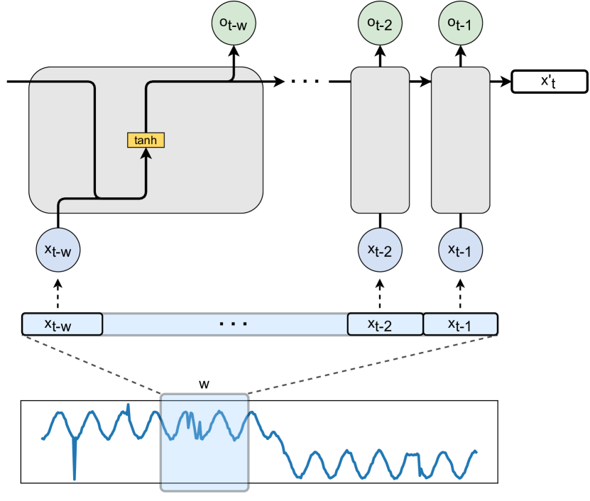
(a) RNN

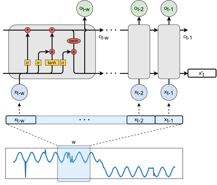
(b) LSTM

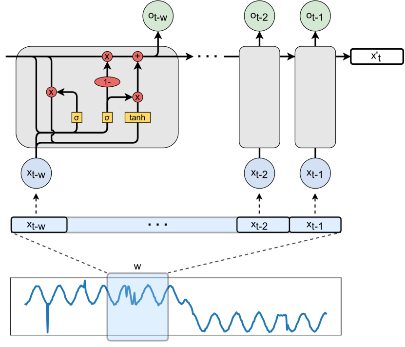
(c) GRU

Figure 5. An Overview of (a) Recurrent neural network (RNN), (b) Long short-term memory unit (LSTM), and (c) Gated recurrent unit (GRU). These models can predict $x_{t}^{\prime}$ by capturing the temporal information of a window of $w$ samples prior to $x_{t}$ in the time series. Using the error $|x_{t}-x_{t}^{\prime}|$, an anomaly score can be computed.

3.2.1. Recurrent Neural Network (RNN)

Since RNNs have internal memory, they can process input sequences of variable length and exhibit temporal dynamics (Tealab, 2018), (Abiodun et al., 2018). An example of a simple RNN architecture can be seen in Fig. 5(a). Recurrent units take the points of the input window $X_{t-w:t-1}$ and forecast the next timestamp as an output, $x^{\prime}_{t}$. Iteratively, the input sequence is fed to the network timestamp by timestamp. Using the input $x_{t-1}$ to the recurrent unit $o_{t-2}$, and an activation function like $tanh$, the output vector $x^{\prime}_{t}$ is calculated using the following equations:

(10) $$\begin{split}x^{\prime}_{t}=\sigma(W_{x^{\prime}}.o_{t-1}+b_{x^{\prime}})\ ,\\ o_{t-1}=\tanh(W_{o}.x_{t-1}+U_{o}.o_{t-2}+b_{h})\end{split}$$

where $W_{x^{\prime}}$, $W_{o}$, $U_{o}$, and $b$ are the parameters of the network. Recurrence occurs when the network uses previous outputs as inputs to remember what it learned from previous steps. This is where the network learns long-term and short-term dependencies.

Long-short-term memory (LSTM) promises to provide memory to RNNs lasting thousands of steps (Hochreiter and Schmidhuber, 1997). As a result of RNN architectures (shown in Fig. 5) with LSTM units, deep neural networks can achieve superior predictions as they incorporated long-term dependencies. There are four main components of an LSTM unit presented in Fig. 5(b): cells, input gates, output gates, and forget gates. During variable time periods, the cell remembers values while the other gates control the flow of information. The processing of a timestamp inside an internal LSTM can be explained in the following equations. At first, the forget gate $f_{t-1}$ is calculated as the output of a sigmoid function with two inputs $x_{t-1}$ and $o_{t-2}$:

(11) $$f_{t-1}=\sigma(W_{f}.x_{t-1}+U_{f}.o_{t-2})$$

The input gate $i_{t-1}$ and output gate $s_{t-1}$ can be obtained as:

(12) $$i_{t-1}=\sigma(W_{i}.x_{t-1}+U_{i}.o_{t-2})$$

(13) $$s_{t-1}=\sigma(W_{s}.x_{t-1}+U_{s}.o_{t-2})$$

Next, in addition to a hidden state $o_{t}$, LSTM has a memory cell named $c_{t-1}$. In order to learn from data and update $c_{t-1}$, $\tilde{c_{t-1}}$ that contains new candidate values should be computed as the output of a $\tanh$ function. After that, $\tilde{c_{t}}$ add it to $c_{t-1}$ to update the memory cell state.

(14) $$\begin{split}\tilde{c_{t-1}}=\tanh(W_{c}.x_{t-1}+U_{c}.o_{t-2})\ ,\\ c_{t-1}=i_{t-1}.\tilde{c_{t-1}}+f_{t-1}.c_{t-2}\end{split}$$

Specifically, $f_{t-1}\in(0,1)$ since it is a sigmoid output. With $f_{t-1}$, $c_{t-2}$ is completely erased when it is close to zero, while it’s completely retained when it’s close to one. For this reason, $f_{t-1}$ is referred to as forget gate. Finally, the hidden state $o_{t-1}$ or the output is obtained by:

(15) $$o_{t-1}=\tanh(c_{t-1}).s_{t-1}$$

Where $W$s and $U$s are the parameters of the LSTM cell. $x^{\prime}_{t}$ is finally calculated using Equation 10.

Experience with LSTM has shown that stacking recurrent hidden layers of sigmoidal activation units in a network captures the structure of time series and allows for processing time series at different time scales compared to the other deep learning architectures (Hermans and Schrauwen, 2013). LSTM-AD (Malhotra et al., 2015) possesses long-term memory capabilities, and for the first time, hierarchical recurrent processing layers have been combined to detect anoamlies in univariate time series without using labels for training. Stacking recurrent hidden layers also facilitate learning higher-order temporal patterns without requiring prior knowledge of their duration. The network predicts several future time steps in order to ensure that it captures the temporal structure of the sequence. Consequently, each point in the sequence has multiple corresponding predicted values from different points in the past, resulting in multiple error values. To assess the likelihood of anomalous behaviour, prediction errors are modelled as a multivariate Gaussian distribution. The LSTM-AD delivers promising outcomes by modelling long-term and short-term temporal relationships. Results from LSTM-AD suggest that LSTM-based prediction models are more effective than RNN-based models when there is no way of knowing whether the normal behaviour involves long-term dependencies. As opposed to the stacked LSTM used in LSTM-AD, Bontemps et al. (2016) use a simple LSTM RNN to propose a model for collective anomaly detection based on LSTM RNN’s predictive capabilities for univariate time series (Hochreiter and Schmidhuber, 1997). In the first step, an LSTM RNN is trained with normal time series before making predictions. Predictions of current events depend on both their current state and their history. By introducing the circular array, the model will be configured to detect collective anomalies, which contains the errors of a subsequence. A collective anomaly will be identified by prediction errors above a threshold in the circular array.

Motivated by promising results in LSTM models for UTS anomaly detection, a number of methods attempt to detect anomalies in MTS based on LSTM architectures. In DeepLSTM (Chauhan and Vig, 2015) training, stacked LSTM recurrent networks are used to train on normal time series. After that, using maximum likelihood estimation, the prediction error vectors are fitted to a multivariate Gaussian. The model is then applied to predict the mixture of both anomalous and normal validation data, and the Probability Density Function (PDF) values of the associated error are recorded. This approach has the advantage of not requiring preprocessing, and it works directly on raw time series. LSTM-PRED (Goh et al., 2017) is based on three LSTM stacks with 100 hidden units each, and input sequences of data for 100 seconds are used as a predictive model to learn temporal dependencies. The Cumulative Sum (CUMSUM) method is used to detect anomalies rather than computing thresholds for every sensor. CUSUM calculates the cumulative sum of the sequence predictions to detect slight deviations, reducing false positives. After computing both positive and negative differences between the predicted values and actual data, an Upper Control Limit (UCL) and a Lower Control Limit (LCL) from the validation dataset are determined and act as boundary controls to decide whether an anomaly has occurred. Moreover, this model can localise the sensor exhibiting abnormal behaviour.

In all three above-mentioned models, LSTMs were stacked; however, LSTM-NDT (Hundman et al., 2018) combines various techniques. LSTM and RNN achieve high prediction performance by extracting historical information from MTS. There is a nonparametric, dynamic, and unsupervised threshold finding technique presented in the article that can be used for evaluating residuals. By applying this approach, thresholds can be set automatically for evolving data in order to address diversity, instability, and noise issues. (Ding et al., 2019) proposes a method called LSTM-BP based on LTSM and improves the internal structure of LSTM for detecting time series anomalies. A real-time anomaly detection algorithm called LGMAD for complex systems combining LSTM and Gaussian Mixture Model (GMM) is presented in this paper. The first step is to use LSTM to detect anomalies in univariate time series data, and then a Gaussian Mixture Model is adopted in order to provide a multidimensional joint detection of potential anomalies. Aside from that, to increase the model’s performance, the health factor $\alpha$ concept is introduced to describe the system’s health status. This model can only be applied in low-dimensional applications. For the case of high-dimensional anomaly detection, the proposed method can be used by dimensionality reduction techniques, such as principle component analysis (PCA) to detect anomalies (Huang et al., 2006), (Papadimitriou et al., 2005).

Ergen and Kozat (2019) present LSTM-based anomaly detection algorithms in an unsupervised framework, as well as semi-supervised and fully supervised frameworks. To detect anomalies, it uses scoring functions implemented by One Class-SVM (OC-SVM) and Support Vector Data Description (SVDD) algorithms. In this framework, LSTM and OC-SVM (or SVDD) architecture parameters are jointly trained with well-defined objective functions, utilizing two joint optimisation approaches. The gradient-based joint optimisation method uses revised OC-SVM and SVDD formulations, illustrating their convergence to the original formulations. As a result of the LSTM-based structure, methods are able to process data sequences of variable length. Aside from that, the model is effective at detecting anomalies in time series data without preprocessing. Moreover, since the approach is generic, the LSTM architecture in this model can be replaced by a GRU (gated recurrent neural networks) architecture (Chung et al., 2014).

GRU was proposed by Cho et al. (2014) in 2014, similar to LSTM but incorporating a more straightforward structure that leads to less computing time (see Fig. 5(c)). Both LSTM and GRU use gated architectures to control information flow. However, GRU has gating units that inflate the information flow inside the unit without having any separate memory unit, unlike LSTM (Dey and Salem, 2017). There is no output gate but an update gate and a reset gate. Fig. 5(c) shows the GRU cell that integrates the new input with the previous memory using its reset gate. The update gate defines how much of the last memory to keep (Gulli and Pal, 2017). The issue is that LSTMs and GRUs are limited in learning complex seasonal patterns in multi-seasonal time series. As more hidden layers are stacked and the backpropagation distance (through time) is increased, accuracy can be improved. However, training may be costly. In this regard, AD-LTI (Wu et al., 2020) is suggested. It is a forecasting model that integrates a GRU network using a time series decomposition method called Prophet (Taylor and Letham, 2018), to enable robust learning on seasonal time series data without labels. By conducting time series decomposition before running the prediction model, the seasonal features of input data are explicitly fed into a GRU network. During inference, time series in addition to its seasonality characteristics (such as weekly and daily terms) are given to the model. Furthermore, since projections are based on previous data, which may contain anomalous points, they may not be reliable.In order to estimate the likelihood of anomalies, a new metric called Local Trend Inconsistency (LTI) is proposed. By weighing the prediction made based on a frame at the recent time point with its probability of being normal, LTI overcomes the issue that there might be anomalous frames in history.

Traditional one-class classifiers develop for input data with fixed dimensions and are unable to capture the underlying temporal dependency appropriately for time series data (Ruff et al., 2018). A recent model used recurrent networks to address this issue. THOC (Shen et al., 2020) represents a self-supervised temporal hierarchical one-class network, which consists of a multilayer dilated RNN and a hierarchical SVDD (Tax and Duin, 2004). Multi-scale temporal features are captured using dilated RNNs (Chang et al., 2017) with skip connections. A hierarchical clustering mechanism is applied to merge output of intermediate layers of the dilated RNN rather than only using the lowest-resolution features at the top. Several hyperspheres exhibit normal behaviour in each resolution, which captures real-world time series complexity better than deep SVDD. This facilitates the model to be trained end-to-end, and anomalies are detected using a score, which measures how current values differ from hypersphere representations of normal behaviour. In spite of the accomplishments of RNNs, they can be inefficient for processing long sequences as they are limited to the size of the window.

3.2.2. Convolutional Neural Network (CNN)

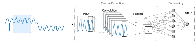
Figure 6. Structure of Convolutional Neural Network (CNN) to predict the next values of input time series based on a window of input data. Since time series are time-dependent by nature, it can only use the inputs it has observed before in predicting the output $x^{\prime}_{t}$ for some time step $t$.

Convolutional neural networks (CNNs) are modified versions of multilayer perceptions that regularise in a different way. The hierarchical pattern in data allows them to construct increasingly complex patterns using smaller and simpler patterns. CNN comprises multiple layers, including convolutional, pooling, and fully connected layers depicted in Fig. 6. Convolutional layers consist of a set of learnable kernels extending across the entire input. Filters are convolved over the input dataset to produce a 2D activation map by computing the dot product between their entries and the input. The pooling operation statistically summarises convolutional outputs. The CNN-based DeepAnt (Munir et al., 2018) model does not require extensive data in training phase, so it is efficient. This model detects even small deviations in time series temporal patterns and can handle low levels of data contamination (less than 5%) in an unsupervised manner. An anomaly detection model can be applied both to univariate and multivariate time series, and it can identify anomalies such as point anomalies, contextual anomalies, and discords.

In structural data analysis, convolutional networks have proven to be valuable for extracting high level features. Due to the inability of traditional CNNs to deal with the characteristics of sequential data like time series, they are not typically used for this type of data, and therefore by developing a temporal convolutional network (TCN) (Bai et al., 2018), dilation convolution is utilised so that they can adapt to sequential data. Most of the CNN-based models use TCN for time series anomaly detection. Essentially, TCN consists of two principles: it produces outputs of the same length as the input, and it does not use information from the future into the past. For the first point, TCN employs a 1D fully-convolutional network, whose hidden layers are the same size as the input layers. A second point can also be achieved using dilated convolution in which output at time $t$ is convolved only with points from time $t$ and prior. The output of the dilated convolution is based on the following equation:

(16) $$x^{\prime}(t)=(x\ast_{l}f)(t)=\ \sum_{i=0}^{\ k-1}f(i).x_{t-l.i}\$$

where $f$ is a filter with size $k$, $\ast$ indicates convolution with the dilation factor $l$, and $x_{t-l.i}$ provides information of the past.

(He and Zhao, 2019) uses TCN which is trained on normal sequences and is able to predict trends over time. The anomaly scores of points are calculated using a multivariate Gaussian distribution fitted to prediction errors. A skipping connection is employed to achieve multi-scale feature mixture prediction for varying scale patterns.

Ren et al. (2019) combine the Spectral Residual (SR) model with CNN (SR-CNN) to achieve superior accuracy, as the SR model derived from visual saliency detection (Hou and Zhang, 2007). More than 200 Microsoft teams have used this univariate time series anomaly detection service, including Microsoft Bing, Office, and Azure. This model is very fast and detects anomalies from 4 million time series per minute. The TCN-AE (Thill et al., 2020a) uses a convolutional architecture coupled with an autoencoder framework. As opposed to a standard autoencoder, it replaces the dense layer architecture with a more powerful CNN architecture which is also more flexible in terms of input size. The TCN autoencoder uses two temporal convolutional neural networks (TCNs) (Bai et al., 2018) for encoding and decoding. Additionally, the downsampling layer in the encoder and the upsampling layer in the decoder are used.

In many real world applications, quasi-periodic time series (QTS) are frequently generated. For instance, some physiological signals like electrocardiograms (ECGs) are QTSs. An automatic QTS anomaly detection framework (AQADF) is presented in (Liu et al., 2020). It comprises a clustering-based two-level QTS segmentation algorithm (TCQSA) and an attention-based hybrid LSTM-CNN model (HALCM). Specifically, TCQSA aims to accurately and automatically divide QTSs into successive quasi-periods. A two-level clustering process is included in TCQSA. First, TCQSA uses a hierarchical clustering technique, which automates the clustering of candidate points for QTSs without manual intervention, making it generic. This second clustering method removes the clusters caused by outliers in QTS, making TCQSA noise-resistant. HALCM applies stacked bidirectional LSTMs (SB-LSTMs) hybridised with CNNs (TD-CNNs) to extract the overall variation trends and local features of QTS, respectively. Consequently, the fluctuation pattern of QTS can be more accurately characterised. Furthermore, HALCM is further enhanced by three attention mechanisms. Specifically, TAGs are embedded in LSTMs in order to fine-tune variations extracted from different parts of QTS. A feature attention mechanism (FAM) and a location attention mechanism (LAM) are embedded into a CNN in order to enhance the effects of key features extracted from QTSs. HALCM can therefore acquire more accurate feature representations of QTS fluctuation patterns.

3.2.3. Graph Neural Network (GNN)

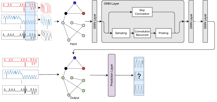
Figure 7. The basic structure of Graph Neural Network (GNN) for multivariate time series anomaly detection that can learn the relationships (correlations) between metrics and predict the expected behaviour of time series.

In the past few years, researchers proposed to extract spatial information from MTS and form a graph structure. Then the problem of time series anomaly detection is converted to detect anomalies of time series given their graph structures and GNNs have been used to model those graphs. The structure of GNNs is shown in Fig. 7. In GNNs, pairwise message passing is the key approach, so that graph nodes iteratively update their representations by exchanging information with each other. In the models for MTS anomaly detection, each dimension (metric) is represented as a single node in the graph and we represent our node set as $V={1,\ldots,d}$. $E$ represents edges in the graph, and they indicate correlations learned from MTS. For node $u/inV$, the message passing layer outputs the following for iteration $k+1$:

(17) $$\begin{split}{h}_{u}^{k+1}=UPDATE^{k}(h_{u}^{k},\ m_{N(u)}^{k})\ ,\\ m_{N(u)}^{k}=AGGREGATE^{k}({h}_{i}^{k},\ \forall i\in N(u))\end{split}$$

where $h_{u}^{k}$ is the embedding corresponding to each node and $N(u)$ is the set of neighbourhood of node $u$.

The ability of GNNs to learn the spatial structure enhances the modelling of multivariate time series data containing correlations. Generally, GNNs presume that the state of each node is affected by the states of its neighbours (Scarselli et al., 2008). A wide variety of GNN architectures have been proposed, implementing different types of message passing. The graph convolution network (GCN) (Kipf and Welling, 2016) models a node’s feature representation by aggregating its one-step neighbours. Graph attention networks (GATs) (Veličković et al., 2017) are based on this approach, but instead of using a simple weight function for every neighbour, they use an attention function to compute different weights for each neighbours.

As previously mentioned, incorporating relationships between features into models would be extremely beneficial. Deng and Hooi (2021) introduce GDN, a graph neural network attention-based that embeds vectors to capture individual sensor characteristics as nodes and captures sensors’ correlations (spatial information) as edges in the graph, which learns to predict sensor behaviour based on attention functions over their adjacent sensors. It is able to detect and interpret deviations from them based on subgraphs, attention weights, and a comparison of predicted and actual behaviour without supervision. An anomaly detection framework called GANF (Graph-Augmented Normalizing Flow) (Dai and Chen, 2022) augments a normalizing flow with graph structure learning. Normalizing flows is a deep generative model for unsupervised learning of the underlying distribution of data and resolving the challenge of label scarcity. Since normalizing flows provides an estimate of the density of any instance, it can be applied to the hypothesis that anomalies tend to fall in low-density areas. GANF is represented as a Bayesian network, which models time series’ conditional dependencies. By factoring multiple time series densities across temporal and spatial information, it learns the conditional densities resulting from factorisation with a graph-based dependency encoder. To ensure that the corresponding graph is acyclic, the authors impose a differentiable constraint on the graph adjacency matrix (Yu et al., 2019). The graph adjacency matrix and flow parameters can both be optimised using a joint training algorithm. After that, Graph-based dependency decoders are used to summarise the conditional information needed to calculate series density. Anomalies are detected by identifying instances with low density. Due to graph structures’ usefulness as indicators of distribution drift, the model provides insights into how distribution drifts in time and how graphs evolve.

Before concluding GNN models we would like to highlight that extracting graph structures from time series and modeling them using GNNs enable the anomaly detection model to learn the changes in spatial information over time which is a promising future research direction.

3.2.4. Hierarchical Temporal Memory (HTM)

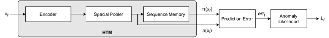
(a) Components of anomaly detection using HTM

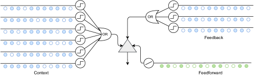
(b) Structure of HTM cell

Figure 8. (a) Components of a Hierarchical Temporal Memory (HTM) based anomaly detection system. Based on the output of an HTM system, it calculates the prediction error and anomaly likelihood measure. (b) An HTM cell internal structure. In HTM cells, dendrites are modelled as overlapped detectors with synapses between them. The context dendrites receive lateral input from other neurons in the layer. If lateral activity on a context dendrite is sufficient, the cell enters a predicted state.

A notable instance of using hierarchical temporal processing for anomaly detection is the Hierarchical Temporal Memory (HTM) system that attempts to mimic the hierarchy of neuron cells, regions, and levels in the neocortex (George, 2008). As Fig. 8(a) illustrates typical HTM algorithm components. The input, $x_{t}$, is fed to an encoder and then a sparse spatial pooling process (Cui et al., 2017). As a result, $a(x_{t})$ represents the current input as a sparse binary vector. Sequence memory forms the core of the system that models temporal patterns in $a(x_{t})$ and returns a prediction in the form of sparse vector $\pi(x_{t})$. Thus, prediction error can be defined as follows:

(18) $$err_{t}=1-\dfrac{\pi(x_{t-1}).a(x_{t})}{|a(x_{t})|}$$

where $|a(x_{t})|$ is the total numbers of 1 in $a(x_{t})$.

Based on the model’s prediction history and the distribution of errors, anomaly likelihood is a probabilistic metric that indicates whether the current state is anomalous or not, as shown in Fig. 8(a). In HTM sequence memory, a column of HTM neurons are arranged in a layer (Fig. 8(b)). There may be several regions within a single level of the hierarchy. At higher hierarchical levels, fewer regions are involved, and patterns learned at lower levels are combined to recall more complex patterns. HTM regions all serve the same purpose. Sensory data enters lower-level regions during the learning stages, and the lower-level regions output the resulting pattern of a specific concept in generation mode. At the top level, the most general and enduring concepts are stored in a single region. In inference mode, a region interprets information coming up from its children as probabilities. As well as being robust to noise, HTM has a high capacity and can simultaneously learn multiple patterns. A spatial pattern in HTM regions is learned by recognizing and memorizing frequent sets of input bits. In the following phase, it identifies sequences of spatial patterns that are likely to occur in succession over time.

Numenta HTM (Ahmad et al., 2017) detects temporal anomalies of univariate time series in predictable and noisy domains using HTM. Consequently, the system is efficient, can handle extremely noisy data, adapts continuously to changes in data statistics, and detects small anomalies without generating false positives. Multi-HTM (Wu et al., 2018) is a learning model that learns context over time, so it is tolerant of noise. Data patterns are learned continuously and predictions are made in real-time, so it can be used for adaptive models. With it, a wide range of anomaly detection problems can be addressed, not just certain types. In particular, it is used for univariate problems and applied efficiently to multivariate time series. The purpose of RADM (Ding et al., 2018) is to present a framework for real-time unsupervised anomaly detection in multivariate time series, which combines HTM with a naive Bayesian network (BN). Initially, the HTM algorithm is used to detect anomalies in UTS with excellent results in terms of detection and response times. The second step consists of combining the HTM algorithm with BN to detect MTS anomalies as effectively as possible without reducing the number of dimensions. As a result, some anomalies that are left out of UTS can be detected, and detection accuracy is increased. BNs are utilised to refine new observations because they are easy to use in specifying posterior probabilities and are adaptive. Additionally, this paper defines a health factor $\alpha$ (a measure of how well the system is running) in order to describe the health of the system and improve detection efficiency.

3.2.5. Transformers

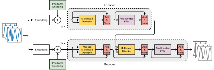
Figure 9. Structure of transformer network for anomaly detection. The Transformer emulates neural sequence models by using an encoder-decoder structure. There are multiple identical blocks in both encoders and decoders. Each encoder block consists of a multi-head self-attention module and a position-wise feedforward network. During decoding, cross-attention models are interposed between the multi-head self-attention module and the position-wise feedforward network. A Transformer does not contain any recurrence or convolution, unlike a recurrent neural network. Rather than modelling sequence information directly, it employs the positional encoding added to the embeddings of the inputs.

Transformers (Vaswani et al., 2017) are deep learning models that weigh input data differently depending on the significance of different parts. In contrast to RNNs, transformers process the entire data simultaneously. Due to its architecture based solely on attention mechanisms, illustrated in Fig. 9, it can capture long-term dependencies while being computationally efficient. Recent studies utilise them to detect time series anomalies as they process sequential data for translation in text data.

The original transformer architecture is encoder-decoder based. An essential part of the transformer’s functionality is its multi-head self-attention mechanism, stated in the following equation:

(19) $$Q,K,V=softmax({\frac{QK^{\mathrm{T}}}{\sqrt{d_{k}}}})V$$

where $Q$, $K$ and $V$ are defined as the matrices and $d_{k}$ is for normalisation of attention map.

A semantic correlation is detected in a long sequence, and the important elements are filtered from the irrelevant ones. Since transformers have no recurrence or convolution, it is necessary to specify the relative or absolute positions of tokens in the sequence, which is called positional encoding. GTA (Chen et al., 2021a) greatly benefits from the sequence modelling ability of the transformer and employs a bidirectional graph structure to learn the relationship among multiple IoT sensors. A novel Influence Propagation (IP) graph convolution is proposed as an automatic semi-supervised learning policy for graph structure of dependency relationships between sensors. As part of the training process to discover hidden relationships, the neighbourhood field of each node is constrained to further improve inference efficiency. Following that, they are fed into graph convolution layers for modelling information propagation. As a next step, a multiscale dilated convolution and a graph convolution are fused to provide a hierarchical temporal context encoding. They use transformer-based architectures to model and forecast sequences due to their parallelism and capability to capture contextual information. The authors also propose an alternative method of reducing multi-head attention’s quadratic complexity using multi-branch attention. In another recent work they use transformer with stacked encoder-decoder structures made up solely of attention mechanisms. The SAnD (Simply Attend and Diagnose) (Song et al., 2018) uses attention models to model clinical time series, eliminating the need for recurrence. The architecture utilises the self-attention module, and dependencies within neighbourhoods are captured and designed with multiple heads. Moreover, positional encoding techniques and dense interpolation embedding techniques are used to represent the temporal order. This was also extended to handle multiple diagnoses by creating a multitask variant.

3.3. Reconstruction-based models

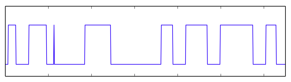
(a) Predictable

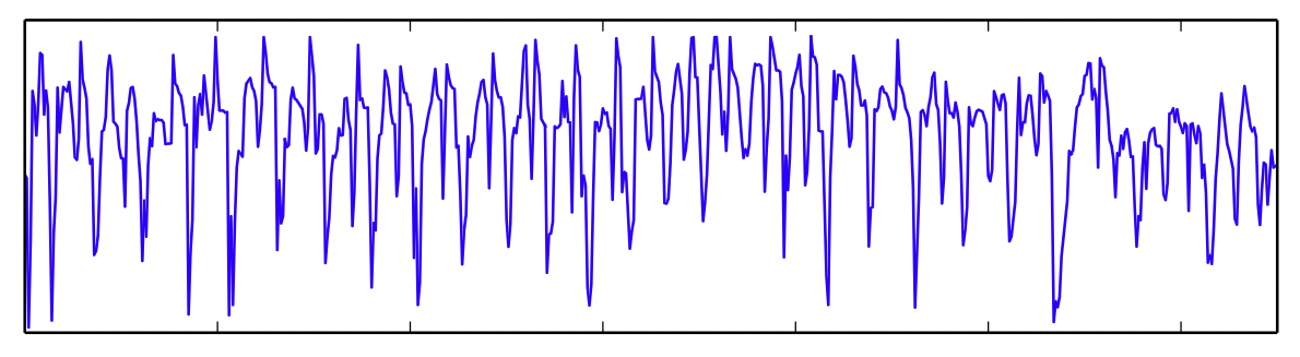
(b) Unpredictable

Figure 10. A time series may be unknown at any given moment or may change rapidly like (b) which illustrates sensor readings for manual control (Malhotra et al., 2016). Such a time series cannot be predicted in advance, making prediction-based anomaly detection ineffective.

Most of the complex time series anomaly detection methods are based on modelling the time series to predict future values and prediction errors. Even so, there is no robust forecasting-based model that can produce an accurate model for rapidly and continuously changing time series (see Figure 10) (Golestani and Gras, 2014) as a time series may be unknown at any given moment or may change rapidly like Figure 10-b. Such a time series cannot be predicted in advance, making prediction-based anomaly detection ineffective. Forecasting-based models dramatically increase prediction error as the number of time points increases, as seen in (Malhotra et al., 2015). Due to this, existing models make very short-term predictions in order to achieve acceptable accuracy since they are incapable of detecting subsequence anomalies. For example, most financial time series predictions can only predict the next step, which is not beneficial if a financial crisis is likely to occur. To overcome this deficiency in forecasting-based models, reconstruction-based models may be more effective.

Models for normal behaviour are constructed by encoding subsequences of normal training data in latent spaces (low dimensions). Model inputs are sliding windows (see Section 3) that provide the temporal context of the reconstruction process. It is not possible for the model to reconstruct anomalous subsequences in the test phase since it is only trained on normal data (semi-supervised). As a result, anomalies are detected by reconstructing a point/sliding window from test data and comparing them to the actual values, called reconstruction error. In some models, detection of anomalies is triggered when the reconstruction probability is below a specified threshold since anomalous points/subsequences have a low reconstruction probability.

3.3.1. Autoencoder (AE)

The autoencoder (AE), referred to as autoassociative neural networks (Kramer, 1991), has been extensively studied in the form of a neural network with nonlinear dimensionality reduction capability in MTS anomaly detection (Sakurada and Yairi, 2014), (Zong et al., 2018). Recent deep learning developments have emphasised on learning of low-dimensional representations (encoding) using AE (Hinton and Salakhutdinov, 2006), (Bhatia et al., 2021). Autoencoders consist of two components (see Fig. 11(a)): an encoder that converts input into encoding and a decoder that reconstructs input from the encoding. It would be ideal if an autoencoder could perform accurate reconstruction and minimise reconstruction error. This approach can be summarised as follows:

(20) $$Z_{t-w:t}=Enc(X_{t-w:t},\phi),\hat{X}_{t-w:t}=Dec(Z_{t-w:t},\theta)$$

where $X_{t-w}$ is a sliding window as shown in Fig. 11(a) and $x_{t}\in R^{d}$. $E$ is the encoder network with $\phi$ parameters, so $Z$ is the representation in the bottleneck of the AE, which is called latent space. After that, this encoding window is fed into the decoder network, named $D$, with $\theta$ parameters and gives $\hat{X}_{t-w}$ as a reconstruction of $X$. In the training phase, encoder and decoder parameters are updated according to the following:

(21) $$(\phi^{*},\theta^{*})=arg\ \underset{\phi,\theta}{m}in\ Err(X_{t-w:t},\ Dec(Enc(X_{t-w:t},\ \phi),\ \theta))$$

To capture more information and make better representations of the dominant information, various techniques are offered like Sparse Autoencoder (SAE) (Ng et al., 2011), Denoising Autoencoder (DAE) (Vincent et al., 2008), and Convolutional Autoencoder (CAE) (Noh et al., 2015). The anomaly score of a window in an AE-based model can be defined according to reconstruction error with the following basic function:

(22) $$AS_{w}=||X_{t-w:t}\ -Dec(Enc(X_{t-w:t},\ \phi),\ \theta)||^{2}$$

There are several papers in this category in our study. Sakurada and Yairi (2014) demonstrate the application of autoencoders to dimensionality reductions in MTS as a prepoccessing for anomaly detection, as well as mechanisms for anomaly detection using autoencoders. The method disregards time sequence by considering each data sample at each time index as an independent. Even though autoencoders already perform well without temporal information, they can be further boosted by providing current and past samples. To clarify autoencoder properties, they compare linear PCA, denoising autoencoders (DAEs), and kernel PCA. As a result, authors found that autoencoders detect anomalous components that linear PCA is incapable of detecting, and autoencoders can be enhanced by including denoising autoencoders. Additionally, autoencoders avoid the complex computations that kernel PCA requires without compromising quality and detection quality. DAGMM (Deep Autoencoding Gaussian Mixture Model) (Zong et al., 2018) estimates MTS input sample probability using the Gaussian mixture prior in the latent space in an end-to-end framework. This model consists of two major components: a compression network and an estimation network. The compression network performs dimensionality reduction for input samples with a stochastic deep autoencoder, producing low-dimensional representations based on both the reduced space and the reconstruction error features. The estimation network calculates sample energy (defined next) through Gaussian Mixture Modeling in low-dimensional representations. Sample energy is used to determine reconstruction errors; high sample energy means a high degree of abnormality. Despite this, only spatial dependencies are considered, and no temporal information is included. Through end-to-end training, the estimation network introduced a regularisation term which helps the compression network to avoid local optima and produce low reconstruction errors.

The EncDec-AD (Malhotra et al., 2016) model detects anomalies even from unpredictable univariate time series, in contrast to many existing models for anomaly detection. In this approach, the multivariate time series is reduced to univariate by considering only the first principal component. It has been claimed that it can detect anomalies from time series with lengths up to 500, indicating that LSTM encoder-decoders learn a robust model of normal behaviour. In spite of this, it suffers from an error accumulation problem when it has to decode long sequences of data. (Kieu et al., 2019) proposes two autoencoder ensemble frameworks based on sparsely-connected recurrent neural networks. In one framework, multiple autoencoders are trained independently, while another framework facilitates the simultaneous training of multiple autoencoders using a shared feature space. Both frameworks use the median of the reconstruction errors of multiple autoencoders to measure the likelihood of an outlier in a time series. Audibert et al. (2020) propose Unsupervised Anomaly Detection for Multivariate Time Series (USAD) using autoencoders in which adversarially trained autoencoders are utilised to amplify reconstruction errors. The input for either training or testing is a sequence of observations with a temporal order for retaining this information. Furthermore, adversarial training coupled with its architecture, enables the system to distinguish anomalies while facilitating fast learning. Goodge et al. (2020) determine whether autoencoders are vulnerable to adversarial attacks in anomaly detection by examining the results of a variety of adversarial attacks. Approximate Projection Autoencoder (APAE) is proposed to improve the performance and robustness of the model under adversarial attacks. By using gradient descent on latent representations, this method produces more accurate reconstructions and increases robustness to adversarial threats. As part of this process, a feature-weighting normalisation step takes into account the natural variability in reconstruction errors between different features.

In MSCRED (Zhang et al., 2019c), attention-based ConvLSTM networks are designed to capture temporal trends, and a convolutional autoencoder is used to encode and reconstruct the signature matrix (which contains inter-sensor correlations) instead of relying on the time series explicitly. Matrixes have a length of 16 and a step interval of 5. The reconstruction error of the signature matrix may be used to calculate an anomaly score. It also highlights how to identify root causes and interpret anomaly duration in addition to detecting anomalies. In CAE-Ensemble (Campos et al., 2021), a convolutional sequence-to-sequence autoencoder is presented, which can capture temporal dependencies with high training parallelism. In addition to Gated Linear Units (GLU) incorporated with convolution layers, attention is also applied to capture local patterns by recognising similar subsequences that recur in input, such as periodicity. Since the outputs of separate basic models can be combined to improve accuracy through ensembles (Chen et al., 2017), a diversity-driven ensemble based on CAEs is proposed along with a parameter-transfer-based training strategy instead of training each CAE model separately. In order to ensure diversity, the objective function also considers the differences between basic models, rather than simply assessing their accuracy. Using ensemble and parameter transferring techniques reduces training time and error considerably.

RANSysCoders (Abdulaal et al., 2021) outlines a real-time anomaly detection method used by eBay. The authors propose an architecture that employs multiple encoders and decoders with random feature selection to infer and localise anomalies through majority voting, and decoders determine the bounds of the reconstructions. In this regard, RANCoders are Bootstrapped autoencoders for feature-bounds construction. Furthermore, spectral analysis (Welch, 1967) of the latent space representation is suggested as a way to extract priors for multivariate time series to synchronise raw series representations. Improved accuracy can be attributed to features synchronisation, bootstrapping, quantile loss, and majority vote for anomaly inference. The method overcomes limitations associated with previous work, including a posteriori threshold identification, time window selection, downsampling for noise reduction, and inconsistent performance for large feature dimensions. The authors study the limitations of existing widely used evaluation methods, such as the point-adjust method, and suggest an alternative method to better evaluate anomaly detection models’ effectiveness in practice.

A novel Adaptive Memory Network with Self-supervised Learning (AMSL) AMSL (Zhang et al., 2022) is proposed for increasing the generalisation capacity of unsupervised anomaly detection. An autoencoder framework using convolutions can enable end-to-end training. AMSL integrates self-supervised learning and memory networks in order to overcome the challenges of limited normal data. As a first step, the encoder maps the raw time series and its six transformations into a latent feature space. In order to learn generalised feature representations, a multi-class classifier must be built to classify these feature types. During this process, the features are also fed into global and local memory networks, which can learn common and specific features to improve representation ability. Finally, the adaptive fusion module derives a new reconstruction representation by fusing these features.

(a) Auto-Encoder

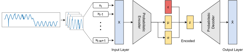
(b) Variational Auto-Encoder

Figure 11. This is the basic structure of (a) Auto-Encoder that compress an input window into a lower-dimensional representation ($h$) and then reconstruct the output $\hat{X}$ from this representation. and (b) Variational Auto-Encoder that receives an input window with size $w$. By compressing it, the encoder creates the latent distribution. Using the sampled data from a parameterised distribution as input, the decoder outputs $\hat{X}$ as close to $X$ as possible.

3.3.2. Variational Autoencoder (VAE)

Fig. 11(b) shows a typical configuration of variational autoencoder (VAE), a directional probabilistic graph model which combines neural network autoencoders with mean-field variational Bayes (Kingma and Welling, 2013). The VAE works similarly to autoencoders, but instead of encoding inputs as single points, it encodes them as a distribution using inference network $q_{\phi}(Z_{t-w+1:t}|X_{t-w+1:t})$ where $\phi$ is its parameters. It represents a $d$ dimensional input $X_{t-w+1:t}$ to a latent representation $Z_{t-w+1:t}$ with a lower dimension $k<d$. A sampling layer takes a sample from a latent distribution and feeds it to the generative network $p_{\theta}(X_{t-w+1:t}|Z_{t-w+1:t})$ with paprameters $\theta$ and its output is $g(Z_{t-w+1:t})$, reconstruction of the input. There are two components of the loss function, as stated in Equation (23), that are minimised in a VAE: a reconstruction error that aims to improve the process of encoding and decoding and a regularisation factor, which aims to regularise the latent space by making the encoder’s distribution as close to the preferred distribution as possible.

(23) $$loss=||X_{t-w+1:t}-g(Z_{t-w+1:t})||^{2}+KL(N(\mu_{x},\sigma_{x}),\ N(0,1))$$

where $KL$ is is the Kullback–Leibler divergence. By using regularised training, it avoids overfitting and ensures that the latent space is appropriate for a generative process.

LSTM-VAE (Park et al., 2018) represents an LSTM-based variational autoencoder that adopts variational inference for reconstruction. In the original VAE, FFN is replaced with LSTM, which is trained with a denoising autoencoding method to improve representation capabilities. This model detects anomalies when the log likelihood of the given data point falls below a threshold. The threshold is dynamic and state-based, which denotes a varying threshold that changes over the estimated state of a task so that false alarms can be reduced. Xu et al. (2018) discover that training on normal and abnormal data is necessary for VAE anomaly detection. The proposed model called Donut is an unsupervised anomaly detection method based on VAE (a representative deep generative model) trained from shuffled training data. Three steps in Donut algorithm, namely, Modified ELBO (evidence lower bound), Missing Data Injection for training, and MCMC (Markov chain Monte Carlo) Imputation (Rezende et al., 2014) for detection, allow it to vastly outperform others for detecting anomalies in seasonal Key Performance Indicators (KPIs). Due to VAE’s nonsequential nature and the fact that data is fed in sliding window format without accounting for their relationship, Donut cannot handle temporal anomalies. Later on, Bagel (Li et al., 2018) is proposed as an unsupervised and robust algorithm to handle temporal anomalies. Instead of using VAE in Donut, Bagel employs conditional variational autoencoder (CVAE) (Lavin and Ahmad, 2015), (Laxhammar et al., 2009) and considers temporal information. VAE models the relationship between two random variables, $x$ and $z$. CVAE models the relationship between $x$ and $z$, conditioned on $y$, i.e., it models $p(x,z|y)$.

STORNs (Sölch et al., 2016), or stochastic recurrent networks, were used to learn a probabilistic generative model of high-dimensional time series data using variational inference (VI). The algorithm is flexible and generic and does not require any domain knowledge when applied to spatially and temporally structured time series. In fact, OmniAnomaly (Su et al., 2019) is a VAE in which stochastic recurrent neural networks are used to learn robust representations of multivariate data, and planar normalizing flow (Rezende and Mohamed, 2015) is used to describe non-Gaussian distributions of latent space. The method computes anomaly detection based on reconstruction probability and quantifies the interpretability of each feature depending on its reconstruction probabilities. It implements the POT method to find an anomaly threshold. InterFusion (Li et al., 2021b) proposes to use a hierarchical Variational Autoencoder (HVAE) with two stochastic latent variables for learning the intermetric and temporal representations; and a two-view embedding by relying on an auxiliary ”reconstructed input” that compresses the MTS along with the metric and time aspects. In order to prevent overfitting anomalies in training data, InterFusion employs a prefiltering strategy in which temporal anomalies are eliminated through a reconstruction process to learn accurate intermetric representations. This paper proposes MCMC imputation multivariate time series for anomaly interpretation and introduces IPS, a segment-wise metric for assessing anomaly interpretation results.

There are a few studies on the anomaly detection of noisy time series data in this category. In an effort to capture complex patterns in univariate KPI with non-Gaussian noises and complex data distributions, Buzz (Chen et al., 2019) introduces an adversarial training method based on partition analysis. This model proposes a primary form of training objectives based on Wasserstein distance and describes how it transforms into a Bayesian model. This is a novel approach to linking Bayesian networks with optimal transport theory. Adversarial training calculates the distribution distance on each partition, and the global distance is the expectation of distribution distance on all partitions. SISVAE (smoothness-inducing sequential VAE) (Li et al., 2020) detects point-level anomalies that are achieved by smoothing before training a deep generative model using a Bayesian method. As a result, it benefits from the efficiency of classical optimisation models as well as the ability to model uncertainty with deep generative models. In this model, mean and variance are parameterised independently for each timestamp, which provides thresholds to be dynamically adjusted according to noise estimates. Considering that time series may change over time, this feature is crucial. A number of studies have used VAE for anomaly detection, assuming a unimodal Gaussian distribution as a prior in the generative process. Due to the intrinsic multimodality distribution of time series data, existing studies have been unable to learn the complex distribution of data. This challenge is addressed by an unsupervised GRU-based Gaussian Mixture VAE presented in (Guo et al., 2018). Using GRU cells, time sequence correlations can be discovered. Afterwards, the latent space of multimodal data is represented by a Gaussian Mixture. Through optimisation of the variational lower bound, the VAE infers latent embedding and reconstruction probability.

In (Zhang et al., 2019b) a VAE with two additional modules is proposed: Re-Encoder and Latent Constraint network (VELC). A re-encoder is added to the VAE architecture to obtain new latent vectors. By employing this more complex architecture, the anomaly score (reconstruction error) can be maximised both in the original and latent spaces so that the normal samples can be accurately modelled. Moreover, a VELC is applied to the latent space, so the model does not reconstruct untrained anomalous observations. Consequently, it generates new latent variables similar to those of training data, which can help it differentiate normal from anomalous data. The VAE and LSTM are integrated as a single component in PAD (Chen et al., 2021c) to support unsupervised anomaly detection and robust prediction. VAE dramatically decreases the effect of noise on prediction units. As for LSTMs, they assist VAE in maintaining the long-term sequences outside of its window. Furthermore, spectral residuals (SR) (Hou and Zhang, 2007) are fed into the pipeline to enhance performance. At each subsequence, SR assigns a weight to the status to show the degree of normality.

A TopoMAD (topology-aware multivariate time series anomaly detector) (He et al., 2020) combines GNN, LSTM, and VAE to detect unsupervised anomalies in cloud systems with spatiotemporal learning. TopoMAD is a stochastic seq2seq model that integrates topological information from a cloud system to produce graph-based representations of anomalies. Accordingly, two representative graph neural networks (GCN and GAT) are replaced as an LSTM cell’s basic layer to capture the topology’s spatial dependencies. Examining partially labelled information has become more imperative in order to detect anomalies (Kingma et al., 2014). In the semi-supervised VAE-GAN (Niu et al., 2020) model, LSTMs are incorporated into VAE as layers to capture long-term patterns. An encoder, a generator, and a discriminator are all trained simultaneously, thereby taking advantage of the encoder’s mapping and the discriminator’s ability. In addition, by combining VAE reconstruction differences with discriminator results, anomalies from normal data can be better distinguished.

Recently, a robust deep state space model (RDSSM) (Li et al., 2022) is developed which is an unsupervised density reconstruction-based model for detecting anomalies in multivariate time series. This model differs from most current anomaly detection methods in that it uses raw data contaminated with anomalies is used during training rather than assumed to be free of anomalies. There are two transition modules to account for temporal dependency and uncertainty. In order to handle variations resulting from anomalies, the emission model employs a heavy-tail distribution error buffering component, which provides robust training on contaminated and unlabeled training data. By using the above generative model, they devise a detection method that handles fluctuating noise over time. Compared with existing methods, this model can assign adaptive anomaly scores for probabilistic detection.

In (Wang et al., 2022), a variational transformer is proposed as a technique for unsupervised anomaly detection in multivariable time series data. Instead of constructing a feature relationship graph to capture correlation information, the model extracts correlation through self-attention. The model’s performance is improved due to the reduced dimensionality of the multivariate time series and sparse correlations between sequences. A transformer’s positional encoding, also known as a global temporal encoding in this model, incorporates time series and periodic data to capture long-term dependencies. Multi-scale feature fusion enables the model to obtain a more robust feature expression by integrating feature information from multiple time scales. With its residual variational autoencoder module, the model encodes hidden space with regularity using robust local features. As a result of the residual structure of the module, the KL divergence is alleviated, and the lower limit to model generation is improved.

3.3.3. Generative adversarial network (GAN)

A generative adversarial network (GAN) is an artificial intelligence algorithm designed for generative modelling based on game theory (Goodfellow et al., 2014), (Goodfellow et al., 2014). In generative models, training examples are explored, and the probability distribution that generated them is learned. In this way, generative adversarial networks can generate more examples based on the estimated distribution, as illustrated in Fig. 12. Assume that we named the generator, $G$ and the discriminator, $D$. In order to train the generator and discriminator, the following minimax game is used:

(24) $$\underset{G}{m}in\ \underset{D}{m}ax\ V(D,G)=\mathbb{E}_{x\sim p(X)}[log\ D(X_{t-w+1:t})]+\mathbb{E}_{z\sim p(Z)}[log(1-D(Z_{t-w+1:t}))]$$

where $p(x)$ is the probability distribution of input data and $X_{t-w+1:t}$ is a sliding window from training set, called real input in Fig.12. Also, $p(z)$ is the prior probability distribution of generated variable and $Z_{t-w+1:t}$ is a generated input window taken from a random space with the same window size.

In spite of the fact that GANs have been applied to a wide variety of purposes (mainly in research), they continue to involve unique challenges and research openings because of relying on game theory which is distinct from most approaches to generative modelling. Generally, GAN-based models take into account the fact that adversarial learning makes the discriminator more sensitive to data outside the current dataset, making reconstructions of such data more challenging. BeatGAN (Zhou et al., 2019) is able to regularise its reconstruction robustly because it utilises a combination of autoencoders and GANs (Goodfellow et al., 2014) in cases where labels are not available. Moreover, using time series warping method improves detection accuracy by speed augmentation in training dataset and robust BeatGAN against variability involving time warping in time series data. Research shows that BeatGAN can detect anomalies accurately in both ECG and sensor data.

However, training of the GAN is usually difficult and requires a careful balance between the discriminator and generator (Kodali et al., 2017). A system based on adversarial training is not suitable for online use due to its instability and difficulty in convergence. With Adversarial Autoencoder Anomaly Detection Interpretation (DAEMON) (Chen et al., 2021b), anomalies are detected based on adversarially generated time series. The training of the DAEMON autoencoder consists of three parts: Multivariate time series are encoded first via a one-dimensional CNN. A prior distribution is applied to the latent vector instead of directly decoding the hidden variable, and an adversarial strategy is used to fit the posterior distribution of the hidden variable to the prior distribution. This is due to the fact that if the model has not observed identical patterns before, directly decoding the latent vectors and using the reconstruction error will not accurately reconstruct the time series. Afterwards, reconstructed time series are generated by a decoder. Another adversarial training procedure is used in parallel to reduce the differences between the original and reconstructed values. It determines the root cause by computing the reconstruction error for each metric and picking the top-k metrics with the highest reconstruction error based on a new metric called Reconstructed Discounted Cumulative Gain (RDCG@P%) which utilises Normalized Discounted Cumulative Gain (NDCG). NDCG is a ranking quality measure that is associated with web search engine algorithms or related applications.

MAD-GAN (Multivariate Anomaly Detection with GAN) (Li et al., 2019) is a model based on Generic Adversarial Networks (GAN). It captures the temporal relations between time series distributions by LSTM-RNN, which is employed as both the generator and discriminator in a GAN and considers the entire data simultaneously to capture the latent interaction between them. For detecting anomalies, reconstruction error and discrimination loss are both used. The FGANomaly (Du et al., 2021) (Filter GAN) reduces the problem of overfitting in conventional AE-based and GAN-based anomaly detection models by screening possible abnormal samples before training using pseudo-labels, which results in capturing normal distributions more accurately. The generator also has an objective called Adaptive Weight Loss, which dynamically assigns weights to different points based on their reconstruction errors during training. By using this training objective, the model can focus more on plausible normal data, thereby alleviating overfitting.

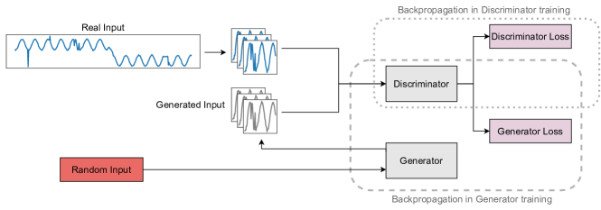
Figure 12. An overview of Generative Adversarial Network (GAN) that consists of two main components: generator and discriminator. The generator constructs fake input windows of time series that are connected directly to discriminator inputs. A discriminator learns to distinguish genuine time series from fake windows by using the generated instances as negative training examples. It is possible to calculate a combined anomaly score by combining both the trained discriminator and the generator.

3.3.4. Transformers

Anomaly Transformer (Xu et al., 2021) with the attention mechanism is proposed to capture the association discrepancy by modelling the prior association and series-association at the same time for each timestamp to make rare anomalies more distinguishable. In this perspective, anomalies are more difficult to connect with the whole series, whereas normality connects more easily with adjacent timestamps. Prior associations estimate adjacent concentration inductive bias using the Gaussian kernel, while series-associations use self-attention weights learned from raw data. In addition to reconstruction loss, a MINIMAX approach is devised to increase the degree of normal-abnormal discrimination of the association discrepancy. TranAD (Tuli et al., 2022) is another transformer-based anomaly detection model that has self-conditioning and adversarial training. As a result of its architecture, it is efficient for training and testing while preserving stability when dealing with huge input. When the deviation is too small, i.e., if the data is close to normal, transformer-based encoder-decoder networks may fail in detecting anomalies. The problem can be overcome by an adversarial training strategy that amplifies the reconstruction errors in TranAD. In addition, self-conditioning for robust multimodal feature retrieval can achieve training stability and facilitate generalisation.

Li et al. (2021a) present an unsupervised method called Dilated Convolutional Transformer GAN (DCT-GAN). In this study, they use a transformer to process time series data, a GAN-based model to reconstruct samples and detect anomalies and dilated CNN structures to extract temporal information from latent spaces. It combines several transformer generators with different scales to obtain coarse-grained and fine-grained information within a GAN-based framework for improving its generalisation capability. The model is made compatible with different kinds of anomalies using a weight-based mechanism to integrate generators. Additionally, MT-RVAE (Wang et al., 2022) significantly benefits from transformer’s sequence modelling and VAE capabilities that are categorised in both of these architectures.

3.4. Hybrid models

These models combine a forecasting-based model with a reconstruction-based model to obtain better time series representations. According to Section 3.2 and Section 3.3, a forecasting-based model uses next timestamp predictions, whereas a reconstruction-based model uses latent representations of the whole time series. It is possible to optimise both models simultaneously by using a joint objective function.

3.4.1. Autoencoder (AE)

By capturing spatiotemporal correlation in multisensor time series, the CAE-M (Deep Convolutional Autoencoding Memory network) (Zhang et al., 2021) can model generalised patterns based on normalised data by undertaking reconstruction and prediction simultaneously. We first build a deep convolutional autoencoder with a Maximum Mean Discrepancy (MMD) penalty to approximate some target distribution in low-dimension and reduce the possibility of overfitting caused by noise and anomalies in training data. For better representation of temporal dependencies, nonlinear bidirectional LSTMs with attention and linear autoregressive models are utilised. Neural System Identification and Bayesian Filtering (NSIBF) (Feng and Tian, 2021) is a novel density-based time series anomaly detection framework for Cyber Physical Security (CPS). An end-to-end trained neural network with a specialised architecture is implemented using a state-space model, which tracks the hidden state’s uncertainty over time recursively, to capture CPS dynamics. As part of the detection phase, Bayesian filtering is automatically applied on top of the ”identified” state-space model in order to screen out hidden states and estimate the likelihood of observed values. As a result of the expressive power of neural networks combined with the ability of Bayesian filters to track uncertainty, NSIBF can detect anomalies in noisy sensor data from complex CPS with high accuracy.

3.4.2. Recurrent Neural Network (RNN)

With TAnoGan (Bashar and Nayak, 2020), they have developed a method that can detect anomalies in time series if a limited number of examples are provided. TAnoGan has been evaluated using 46 NAB time series datasets covering a range of topics. Experiments have shown that LSTM-based GANs can outperform LSTM-based GANs when challenged with time series data through adversarial training.

3.4.3. Graph Neural Network (GNN)

In (Zhao et al., 2020), two parallel graph attention (GAT) layers are proposed for self-supervised multivariate time series anomaly detection, which will extract correlations between different time series (intermetric dependencies) and learn the relationships between timestamps (temporal dependencies). This model incorporates both forecasting- and reconstruction-based models by defining an integrated objective. The forecasting model predicts only one point, while the reconstruction model learns a latent representation of the entire time series. The model can diagnose anomalous time series (interpretability). Fused Sparse Autoencoder and Graph Net (FuSAGNet) (Han and Woo, 2022) is a framework that fused both SAE reconstruction and GNN forecasting to discover complex types of anomalies in multivariate data. FuSAGNet incorporates GDN (Deng and Hooi, 2021), but embeds sensors in each process, followed by recurrent units to capture temporal dependencies. By learning recurrent sensor embeddings and sparse latent representations of input, the GNN predicts expected behaviours in test time.

4. Datasets

Table 3. Public dataset and benchmarks used mostly for anomaly detection in time series. There are direct hyperlinks to their names in the first column.

Dataset/Benchmark	Real/Synth	MTS/UTS1	# Samples2	# Entities3	# Dim4	Domain
CalIt2 (Dua and Graff, 2017)	Real	MTS	10,080	2	2	Urban events management
CAP (Terzano et al., 2001) (Goldberger et al., 2000)	Real	MTS	921,700,000	108	21	Medical and health
CICIDS2017 (Sharafaldin et al., 2018)	Real	MTS	2,830,540	15	83	Server machines monitoring
Credit Card fraud detection (Dal Pozzolo et al., 2015)	Real	MTS	284,807	1	31	Fraud detectcion
DMDS (Warszawska, 2020)	Real	MTS	725,402	1	32	Industrial Control Systems
Engine Dataset (Dau et al., 2018)	Real	MTS	NA	NA	12	Industrial control systems
Exathlon (Jacob et al., 2020)	Real	MTS	47,530	39	45	Server machines monitoring
GECCO IoT (Moritz et al., 2018)	Real	MTS	139,566	1	9	Internet of things (IoT)
Genesis (von Birgelen and Niggemann, 2018)	Real	MTS	16,220	1	18	Industrial control systems
GHL (Filonov et al., 2016)	Synth	MTS	200,001	48	22	Industrial control systems
IOnsphere (Dua and Graff, 2017)	Real	MTS	351		32	Astronomical studies
KDDCUP99 (Discovery and Competition, 1999)	Real	MTS	4,898,427	5	41	Computer networks
Kitsune (Dua and Graff, 2017)	Real	MTS	3,018,973	9	115	Computer networks
MBD (He et al., 2020)	Real	MTS	8,640	5	26	Server machines monitoring
Metro (Dua and Graff, 2017)	Real	MTS	48,204	1	5	Urban events management
MIT-BIH Arrhythmia (ECG) (Moody and Mark, 2001) (Goldberger et al., 2000)	Real	MTS	28,600,000	48	2	Medical and health
MIT-BIH-SVDB (Greenwald et al., 1990) (Goldberger et al., 2000)	Real	MTS	17,971,200	78	2	Medical and health
MMS (He et al., 2020)	Real	MTS	4,370	50	7	Server machines monitoring
MSL (Hundman et al., 2018)	Real	MTS	132,046	27	55	Aerospace
NAB-realAdExchange (Ahmad et al., 2017)	Real	MTS	9,616	3	2	Business
NAB-realAWSCloudwatch (Ahmad et al., 2017)	Real	MTS	67,644	1	17	Server machines monitoring
NASA Shuttle Valve Data (Ferrell and Santuro, 2005)	Real	MTS	49,097	1	9	Aerospace
OPPORTUNITY (Dua and Graff, 2017)	Real	MTS	869,376	24	133	Computer networks
Pooled Server Metrics (PSM) (Abdulaal et al., 2021)	Real	MTS	132,480	1	24	Server machines monitoring
PUMP (sensor data, 2018)	Real	MTS	220,302	1	44	Industrial control systems
SMAP (Hundman et al., 2018)	Real	MTS	562,800	55	25	Environmental management
SMD (Li et al., 2018)	Real	MTS	1,416,825	28	38	Server machines monitoring
SWAN-SF (Angryk et al., 2020)	Real	MTS	355,330	5	51	Astronomical studies
SWaT (Mathur and Tippenhauer, 2016)	Real	MTS	946,719	1	51	Industrial control systems
WADI (Ahmed et al., 2017)	Real	MTS	957,372	1	127	Industrial control systems
NYC Bike (Lyft, 2022)	Real	MTS/UTS	+25M	NA	NA	Urban events management
NYC Taxi (Taxi and Commission, 2022)	Real	MTS/UTS	+200M	NA	NA	Urban events management
UCR (Dau et al., 2018)	Real/Synth	MTS/UTS	NA	NA	NA	Multiple domains
Dodgers Loop Sensor Dataset (Dua and Graff, 2017)	Real	UTS	50,400	1	1	Urban events management
KPI AIOPS (Challenges, 2018)	Real	UTS	5,922,913	58	1	Business
MGAB (Thill et al., 2020b)	Synth	UTS	100,000	10	1	Medical and health
MIT-BIH-LTDB (Goldberger et al., 2000)	Real	UTS	67,944,954	7	1	Medical and health
NAB-artificialNoAnomaly (Ahmad et al., 2017)	Synth	UTS	20,165	5	1	-
NAB-artificialWithAnomaly (Ahmad et al., 2017)	Synth	UTS	24,192	6	1	-
NAB-realKnownCause (Ahmad et al., 2017)	Real	UTS	69,568	7	1	Multiple domains
NAB-realTraffic (Ahmad et al., 2017)	Real	UTS	15,662	7	1	Urban events management
NAB-realTweets (Ahmad et al., 2017)	Real	UTS	158,511	10	1	Business
NeurIPS-TS (Lai et al., 2021)	Synth	UTS	NA	1	1	-
NormA (Boniol et al., 2021)	Real/Synth	UTS	1,756,524	21	1	Multiple domains
Power Demand Dataset (Dau et al., 2018)	Real	UTS	35,040	1	1	Industrial control systems
SensoreScope (Barrenetxea, 2019)	Real	UTS	621,874	23	1	Internet of things (IoT)
Space Shuttle Dataset (Dau et al., 2018)	Real	UTS	15,000	15	1	Aerospace
Yahoo (Inc., 2021)	Real/Synth	UTS	572,966	367	1	Multiple domains

¹ MTS/UTS: Multivariate/Univariate, ² $\#$ samples: total number of samples, ³ $\#$ Entities: number of distinct time series, ⁴ $\#$ Dim: number of metrics in MTS

This section summarises datasets and benchmarks for time series anomaly detection which provides a rich resource for researcher in time series anomaly detection. Some of these datasets are single-purpose datasets for anomaly detection, and some are general-purpose time series datasets that we can use in anomaly detection model evaluation with some assumptions or customisation. We can characterise each dataset or benchmark based on multiple aspects and their natural features. Here we collect 48 well-known and/or highly-cited datasets examined by classic and state-of-the-art deep models for anomaly detection in time series. These datasets are characterised based on the below attributes:

• Nature of the data generation which can be real, synthetic or combined.

• Number of entities, which means the number of independent time series inside each dataset.

• Type of variety for each dataset or benchmark, which can be multivariate, univariate or a combination of both.

• Number of dimensions, which is the number of features of an entity inside the dataset.

• Total number of samples of all entities in the dataset.

• The application domain of the dataset.

Note some datasets have been updated by their authors and contributors occasionally or regularly over time. We considered and reported the latest update of the datasets and their attributes. Table 3 shows all 48 datasets with all mentioned attributes for each of them. It also includes hyperlinks to the primary source to download the latest version of the datasets.

More detailed information about these datasets can be found on this Github repository: https://github.com/zamanzadeh/ts-anomaly-benchmark.

5. Application Areas of Deep Anomaly Detection in Time Series

An application typically generates data through a series of generating processes, which further reflect system operations or provide observational information about entities. The result of abnormal behaviour by the generating process is an anomaly. In other words, anomalies often reveal abnormal characteristics of the systems and entities used to generate data. By recognizing these unusual characteristics, we can gain useful insight from different application. The following deep models are classified by the applications they are used for.

5.1. Internet Of Things (IoT)

As part of the smart world, the Internet of Things (IoT) is playing an increasingly significant role in monitoring various industrial equipment used in power plants and handling emergency situations (Qiu et al., 2017). Analysing data anomalies can identify environmental circumstances that require human attention, uncover outliers when cleaning sensor data, or save computing resources by prefiltering undesirable portions of the data. Greenhouse (Lee et al., 2018) applies a multi-step ahead predictive LSTM over high volumes of IoT time series. A semi-supervised hierarchical stacking TCN is presented in (Cheng et al., 2019), which targets the detection of anomalies in smart homes’ communication. Due to their use of offline learning, these approaches are not resistant to changes in input distribution.

In the Industrial Internet of Things (IIoT), massive amounts of data are generated, which are valuable for monitoring the status of the underlying equipment and boosting operational performance. An LSTM-based model is presented in (Zhang et al., 2018) for analysis and forecasting of sensor data from IIoT devices to capture the time span surrounding the failures. (Kim et al., 2018) perform unsupervised anomaly detection using real industrial IIoT time series, such as manufacturing CNC and UCI time series, using a Squeezed Convolutional Variational Autoencoder (SCVAE) deployed in an edge computing environment.

5.2. Server Machines Monitoring and Maintenance

Cloud systems have fueled the development of microservice architecture in the IT industry. There are numerous advantages to this type of architecture, including independent deployment, rapid delivery, and flexibility of expansion (Dragoni et al., 2017). A service failure in such an architecture can cause a series of failures, negatively impacting the customer experience and the company’s revenue. Troubleshooting needs to be performed as soon as possible after an incident. For this reason, continuously monitoring online systems for any anomalies is essential. SLA-VAE (Huang et al., 2022) uses a semi-supervised VAE to identify anomalies in multivariate time series in order to enhance robustness. Using active learning, a framework is designed that can learn and update a detection model online based on a small sample size of highly uncertain data. Cloud server data from two different types of game businesses are used for the experiments. For each cloud server, 11 monitored metrics, such as CPU usage, CPU load, disk usage, and memory usage are adopted.

In the Internet of Things (IoT), wireless sensor networks (WSNs) play a crucial role. Detecting anomalies is essential in this context because it can reveal information about equipment faults and previously unknown events. (Luo and Nagarajan, 2018) introduces an AE-based model to solve anomaly detection problems in WSNs. The algorithm is designed to detect anomalies in sensors locally without requiring communication with other sensors or the cloud. It is evaluated by a real WSN indoor testbed, which consists of 8 sensors, collected over 4 consecutive months with synthetic anomalies.

5.3. Computer Networks

Intrusion detection for computer network systems is becoming one of the most critical tasks for network administrators today. It has an important role for organisations, governments and our society due to the valuable resources hosted on computer networks. Traditional misuse detection strategies are unable to detect new and unknown intrusion types. In contrast, anomaly detection in network security aims to distinguish between illegal or malicious events and normal behaviour of network systems. Anomaly detection can be used to build normal network behaviour and to detect new patterns that significantly deviate from the normal model. Most of the current research on anomaly detection is based on the learning of normal and anomaly behaviours.

The content delivery networks (CDNs) provide websites and cloud services with enhanced user experiences and shorter response times. For managing service quality, CDN operators measure and collect KPIs such as traffic volume, cache hit ratio and server response time to check and diagnose system functionality. SDFVAE (Static and Dynamic Factorised VAE) (Dai et al., 2021) is a noise-tolerant anomaly detection model that learns the KPIs’ latent representations by explicitly factorizing them into two parts that correspond to dynamic and static characteristics.

An essential part of defending a company’s computer networks is the use of network intrusion detection systems (NIDS) to detect different security breaches. The feasibility and sustainability of contemporary networks are challenged by the need for increased human interaction and decreasing accuracy of detection. A NIDS can monitor and analyse network traffic and alarm when intrusions are detected. In (Javaid et al., 2016), using deep learning techniques, they obtain a high-quality feature representation from unlabeled network traffic data. The features are then applied to the supervised classification of normal and anomalous traffic records based on a small but labelled dataset. In this model, a NIDS is developed by employing self-taught learning, a deep learning technique based on sparse autoencoding and soft-max regression. It relies on the KDD Cup 99 dataset (Tavallaee et al., 2009) which is derived from the network traffic, including normal traffic and attack traffic, such as DoS, Probing, and User-to-Root (U2R) and Root-to-Local (R2L). Also, (Alrawashdeh and Purdy, 2016), a Restricted Boltzmann Machine (RBM) and a deep belief network are used for attack (anomaly) detection in KDD Cup 99. S-NDAE (Shone et al., 2018) is trained in an unsupervised manner to extract significant features from the dataset. Unsupervised feature learning with nonsymmetric deep autoencoders (NDAEs) is described in this work. Additionally, it introduces a deep learning classification model constructed by stacking NDAEs and evaluated by datasets like the KDD Cup 99.

With the rapid expansion of mobile data traffic and the number of connected devices and applications, it is necessary to establish a network management system capable of predicting and detecting anomalies effectively. A measure of latency in these networks is the round trip delay (RTT) between a probe and a central server that monitors radio availability. RCAD (Ahmed et al., 2022) presents a distributed architecture for unsupervised detection of RTT anomalies, specifically increases in RTT. It employs the hierarchical temporal memory (HTM) algorithm to build a predictive model.

5.4. Urban Events Management

Traffic anomalies, such as traffic accidents and unexpected crowd gathering, may endanger public safety if not handled timely. Detecting traffic anomalies in their early stage can benefit citizens’ quality of life and city planning. However, traffic anomaly detection faces two main challenges. First, it is challenging to model traffic dynamics due to the complex spatiotemporal characteristics of traffic data. Second, the criteria for traffic anomalies may vary with locations and times. Zhang et al. (2019a) outline a spatiotemporal decomposition framework, which is proposed for detecting urban anomalies. Spatial and temporal features are derived using a graph embedding algorithm to adapt to different locations and times. A three-layer neural network with a fully connected core aggregates spatial and temporal features and estimates the normal component of urban behaviour is a semi-supervised manner.

(Deng et al., 2022) presents a traffic anomaly detection model based on a spatiotemporal graph convolutional adversarial network (STGAN), a spatiotemporal generator and a spatiotemporal discriminator that assesses whether an input sequence is genuine. Spatiotemporal generators can be used to capture the spatiotemporal dependencies of traffic data. There are three independent modules: trend, external, and recent. In the trend module, LSTMs are used to learn long-term temporal features. An external module takes external features as input and is built as a fully-connected layer. Due to the strong spatial and temporal correlations between neighbouring data, a fundamental component of the generator and discriminator is the recent module and graph convolutional gated recurrent unit (GCGRU) is leveraged to help them learn short-term spatiotemporal features. Three modules’ outputs are combined using a graph convolutional network (GCN) layer for the final prediction result. An anomaly score is developed that is location-aware and time-aware.

In order to model dynamic multivariate data effectively, CHAT (Huang et al., 2021b) is devised. In CHAT, the authors model the urban anomaly prediction problem based on hierarchical attention networks. In fact, their architecture combines a bi-directional recurrent layer (BiLSTM) with a temporal-wise attention mechanism to capture the anomaly information relevant for forecasting future anomalies. Additionally, they design an interaction-wise attention mechanism for learning the interactions between regions, anomaly categories and subsequences. Uber uses an end-to-end neural network architecture for uncertainty estimation (Zhu and Laptev, 2017). To improve anomaly detection accuracy, the proposed uncertainty estimate is used to measure the uncertainty of special events (such as holidays). When uncertainty information is incorporated into the anomaly detection model, false positives are reduced during events with high uncertainty, thereby improving accuracy.

One of the most challenging tasks in intelligent transportation systems is forecasting the speed of traffic. The use of navigation systems that predict traffic prior to travel in urban areas can help drivers avoid potential congestion and reduce travel time. The aim of GTransformer (Lu et al., 2022) is to study how GNNs can be combined with attention mechanisms to improve traffic prediction accuracy. Also, TH-GAT (Huang et al., 2021a) is a temporal hierarchical graph attention network designed specifically for this purpose. In general, the concept involves augmenting the original road network with a region-augmented network that can model hierarchical regional structures.

5.5. Astronomical Studies

As astronomical observations and data processing technology advance, an enormous amount of data is generated exponentially. ”Light curves” are generated using a series of processing steps on a star image. Studying light curves contributes to astronomy as a new method for detecting abnormal astronomical events (Li et al., 2001). In (Zhang and Zou, 2018) an LSTM neural network is proposed for predicting light curves.

5.6. Aerospace

Due to the complexity and cost of spacecrafts, failure to detect hazards during flight could lead to serious or even catastrophic destruction. Existance of an anomaly detection system is critical in this case to alert operation engineers when there are no adequate measures. In (Meng et al., 2019), a transformer-based model with two novel components is presented, namely, an attention mechanism that updates timestamps concurrently and a masking strategy that detects anomalies in advance. Testing was conducted on NASA telemetry datasets.

Monitoring and diagnosing the health of liquid rocket engines (LREs) is the most significant concern for spacecraft and vehicle safety, particularly for human launch. Failure of the engine will result directly in the failure of the space launch, resulting in irreparable losses. To achieve reliable and automatic anomaly detection for large equipments such as LREs and multisource data, Feng et al. (2022) suggest using a multimodal unsupervised method for AD with missing sources. In a unified framework composed of several deep AEs and a skip-connected AE, the proposed method integrates intramodal fusion, intermodal fusion, and decision fusion.

5.7. Natural Disasters Detection

The detection of earthquakes in real time requires a high-density network to fully leverage inexpensive sensors. Over the past few years, low-cost acceleration sensors have become widely used for earthquake detection. For the accurate detection of earthquake waveforms in real-time, a detection algorithm must be developed that can analyse and distinguish earthquake waveforms from non-earthquake waveforms. Accordingly, Petrol et al. (Perol et al., 2018) proposed CNNs for detecting earthquakes and locating them from existing earthquake signals recorded by two local stations in Oklahoma. Using deep CNNs, Phasenet (Zhu and Beroza, 2019) is able to determine the arrival time of earthquake waves in archives. In CrowdQuake (Huang et al., 2020), a convolutional-rnn (CRNN) model is proposed as the core detection algorithm. This method relies on hundreds to thousands of low-cost acceleration sensors that are dispersed throughout a large area in order to detect earthquakes in real time. Moreover, past acceleration data can be stored in databases and analysed post-hoc to identify earthquakes that may have been missed by real-time detection. In this model, abnormal sensors can be identified regularly that might compromise earthquake events.

Earthquake prediction relies heavily on earthquake precursor data. Anomalies associated with earthquake precursors can be classified into two main categories: tendency changes and high-frequency mutations. When a tendency does not follow its normal periodic evolution, it is called a changing tendency. Disturbance of high frequency refers to sudden changes in observations that occur with high frequency and large amplitude and often show irregular patterns. Cai et al. (2019) develop a predictive model for normal data by employing LSTM units. Moreover, prediction errors are used to determine whether the behaviour is normal or unusual. Further advantages of LSTM networks include the ability to detect earthquake precursor data without elaborating preprocessing directly.

5.8. Medical and Health

With the widespread adoption of electronic health records, there is an increased emphasis on predictive models that can effectively deal with clinical time series data. As medical technology continues to improve, more proactive approaches are adopted to anticipate and mitigate risks before getting sick, thus further improving the already reliable medical system. These approaches are intended to analyse physiological time series, identify potential risks of illness before they occur, and determine mitigation measures to take. (Wang et al., 2016) uses several convolution layers to extract useful features from the input and then feeds them into a multivariate Gaussian distribution to detect anomalies.

Electrocardiography (ECG) signals are frequently used to assess the health of the heart, and the resulting time series signal is manually analysed by a medical professional to detect any arrhythmia that has occurred. A complex organ like the heart can cause many different arrhythmias. Thus, it would be very beneficial to adopt an anomaly detection approach for analysing ECG signals which are developed in (Kieu et al., 2019), (Zhou et al., 2019) and (Chauhan and Vig, 2015).

Cardiovascular diseases (CVDs) are the leading cause of death in the world. Detecting abnormal heart rates can help doctors to find the CVDs of patients. Using a CNN, Rubin et al. (2017) develop an automated recognition system for unusual heartbeats based on deep learning. In comparison to other popular deep models like CNN, RNNs are more effective at capturing the temporal characteristics of heartbeat sequences. A study on abnormal heartbeat detection using phonocardiography signals is presented in (Rubin et al., 2017). It has been shown that RNNs are capable of producing promising results even in the presence of noise. Also, Latif et al. (2018) uses RNNs because of their ability to model sequential and temporal data even in noisy environments, to detect abnormal heartbeats automatically. (Chen et al., 2020b) proposes a model using the classical echo state network (ESN) (Jaeger, 2007) trained on an imbalanced univariate heart rate dataset, which represents one of the two classic reservoir computing models with a recurrent neural network as a reservoir.

An epilepsy detection framework based on TCN, Gaussian mixture models and Bayesian inference called TCN-GMM (Liu et al., 2019) uses TCN to extract features from EEG time series. In this study, EEG time series datasets without epilepsy were considered normal samples, while those with epilepsy were considered anomalous ones. It is possible to treat Alzheimer’s disease more effectively if the disease is detected early. A 2D-CNN randomised ensemble model is presented in (Lopez-Martin et al., 2020) that uses magnetoencephalography (MEG) synchronisation measures to detect early Alzheimer’s disease symptoms. The proposed detection model is a binary classifier (disease/non-disease) for the time series of MEG activity.

5.9. Energy

It is inevitable that purification and refinement will affect various petroleum products. Regarding this, (Filonov et al., 2016) as an LSTM-based approach is employed to monitor and detect faults in a multivariate industrial time series that includes signals from sensors and control systems of gasoil plant heating loop (GHL). Two stacked LSTM layers are used in this proposed network architecture along with a linear output layer. LSTMs are used to perform sequence-to-sequence prediction based on temporal information. Likewise, according to Wen and Keyes (2019), a CNN is used to detect time-series anomalies using a transfer-learning framework to solve data sparsity problems. The results were demonstrated on the GHL dataset (Filonov et al., 2016), which contains data on cyber-attacks against utility systems.

The use of phasor measurement units (PMU) by utilities for power system monitoring increases the potential for cyberattacks. In (Basumallik et al., 2019), anomalies are detected in multivariate time series data generated by PMU data packets corresponding to different events, such as line faults, trips, generation and load before each state estimation cycle. A CNN-based filter can provide an extra layer of security by removing false data before state estimation. Consequently, it can help operators identify targeted cyber-attacks and make better decisions to ensure grid reliability.

The management of energy in buildings can improve energy efficiency, increase equipment life, as well as reduce energy consumption and operational costs. Fan et al. (2018) propose an autoencoder-based ensemble method for the analysis of energy time series in buildings and the detection of unexpected consumption patterns and excessive waste. Its application to building cooling load and chiller plant electricity consumption has been tested.

5.10. Industrial Control Systems

System calls can be generated through regularly scheduled tasks, which are a consequence of events from a given process, and sometimes, they are caused by interrupts that are triggered by events. Moreover, if the process is event-driven, it can have fast and slow profiles, making it difficult to model its normal behaviour. Similar to this, when modelling a real-time process, the timestamp property is the best way to model the constraint on response time and execution time. It is difficult to construct profiles using system call information since some processes are time-driven, event-driven, or both.

THREAT (Ezeme et al., 2020) provides a deeper insight in anomaly detection in system processes using their properties and system calls. Detecting anomalies at the kernel level provides new insights into the more complex machine-to-machine interactions. This is achieved by extracting useful features from system calls to broaden the scope of anomalies to be detected. Afterwards, a MIMO (multiple-input and multiple-output) architecture is developed to expand the model’s scope and respond to the heightened threat scope that is available with more profound abstractions. In this study, the MIMO-based model and a broadened feature set assist not only in increasing anomaly detection scope but also in helping to understand how one type of anomaly affects the output of another model aimed at detecting a different type of anomaly.

GAN-based anomaly detection and localisation framework (Choi et al., 2020) is proposed along with a transformation method called distance image for multivariate time series. Multivariate time series can be transformed into 2D images to exploit encoders and decoders. The generator can learn a mapping between distance images so that it can analyse both the temporal association of time series data as well as the correlation among multi variables through convolutional filters. A pointwise convolution encoder ensures that the temporal information of each time series is encoded as well as the inter-correlation between the variables. Additionally, residual 2D images can be used for anomaly localisation in images.

An autoencoder based on LSTM was implemented by Hsieh et al. (2019) to detect anomalies in multivariate streams occurring in production equipment components. In this technique, LSTM networks are used to encode and decode actual values and evaluate deviations between reconstructed values and actual values. Using CNN to handle multivariate time series generated from semiconductor manufacturing processes is the basis for the model in (Kim et al., 2019). Further, a MTS-CNN is proposed in (Hsu and Liu, 2021) to detect anomalous wafers and provide useful information for root cause analysis in semiconductor production. A variety of sliding windows of different lengths is generated to improve diversity, and the key features of equipment sensors are learned through stacked convolution-pooling layers.

5.11. Robotics

In the modern manufacturing industry, industrial robots play an increasingly prominent role as they increase productivity and quality. As production lines become increasingly dependent on robots, failures of any robot can cause a plunge into a disastrous situation, while some faults are difficult to identify. Therefore, industrial robots must be maintained to ensure high performance. In order to detect incipient failures in robots before they stop working completely, a real-time method is required to continuously track robots by collecting time series from robots. A sliding-window convolutional variational autoencoder (SWCVAE) is proposed in (Chen et al., 2020a) to detect anomalies in multivariate time series both spatially and temporally in an unsupervised manner.

Many people with disabilities require physical assistance from caregivers, although some human care-giving can be substituted by robots. Robots can help with daily living activities, such as feeding and shaving. In addition, a lack of failure detection systems may lead to a decrease in the usage of robots because of their potential failure cost. By detecting and stopping abnormal task execution in assistance, potential hazards can be prevented or reduced. Analysis in LSTM-VAE (Park et al., 2018) involved 1,555 robot feed executions from 24 individuals, including 12 types of anomalies. STORNs Sölch et al. (2016) is a VAE-based model and recorded the joint configurations of the seven joints of a Rethink Robotics Baxter Robot arm for training and testing. The target distribution consisted of 1000 anomaly-free samples collected at 15 Hz during a pick-and-place task. The 300 samples were collected by manually hitting the robot with random hit commands for testing purposes.

5.12. Environmental management

In ocean engineering, structures and systems are designed in or near the ocean, such as offshore platforms, piers and harbours, ocean wave energy conversion, and underwater life-support systems. As part of the design and site selection phase, long-term historical ocean observations are analysed, and real-time monitoring of the surrounding marine environment is required. The ocean observing system (OOS) provides marine data by using sensors and equipment that work under severe conditions, such as high humidity, salt fog, and vibration. In order to prevent big losses from total machine failure or even natural disasters, it is necessary to detect OOS anomalies early enough. The OceanWNN model (Wang et al., 2019) leverages a novel WNN-based (Wavelet Neural Network) method for detecting anomalies in ocean fixed-point observing time series without any labelled training data. The proposed model can work in real-time, using two methods of detecting new unknown anomalies (observation and prediction). Verification of the proposed method is done by the National Marine Test Site of China.

Wastewater treatment plants (WWTPs) plays a crucial role in protecting the environment. Due to their high energy consumption. However, these plants require an optimum operation to maximise efficiency and minimise energy consumption. Hence, early fault detection and management plays a vital role. A method based on LSTMs was used by (Mamandipoor et al., 2020) to monitor the process and detect collective faults, superior to earlier methods. Moreover, energy management systems must manage gas storage and transportation continuously in order to reduce expenses and safeguard the environment. (Song and Li, 2021) use an end-to-end CNN-based model to implement an internal-flow-noise leak detector in pipes.

6. Discussion and Conclusion

The purpose of this section is to examine some of the major challenges associated with the detection of several types of anomalies in time series that we described in Section 2.4. In contrast to the tasks relating to the majority, regular patterns, anomaly detection focuses on minority, unpredictable and unusual events which brings about some challenges. The following are some challenges that have to be overcome in order to detect anomalies in time series data using deep learning models:

• System behaviour in the real world is highly dynamic and dependent on the environment at the time. Thus, there is a challenge in dealing with time series data due to their non-stationary nature and the changes in data distribution. This means that deep learning models could detect anomalies in real-time.

• The detection of anomalies in multivariate time series data presents a particular challenge as it requires simultaneous consideration of both temporal dependencies and relationships between metrics.

• In the absence of labelled anomalies, unsupervised or semi-supervised approaches are required. Because of this, a large number of normal instances are incorrectly identified as anomalies. Hence, one of the key challenges is finding a mechanism to minimise false positives and improve recall rates of detection. This is regarded as the considerable cost associated with failing to detect anomalies.

• Time series datasets can exhibit significant differences in noise levels, and noisy instances are often irregularly distributed. Thus, models are vulnerable and their performance are severely compromised by noise contained in the input data.

• In scenarios where anomaly detection is being used as a diagnostic tool, a degree of interpretability is required. Even so, anomaly detection research focuses primarily on detection precision, failing to address the issue of interpretability.

• In addition to being rarely addressed in the literature, anomalies that occur on a periodic basis make detection more challenging. A periodic subsequence anomaly is a subsequence that repeats over time (Rasheed and Alhajj, 2013). The periodic subsequence anomaly detection technique, in contrast to point anomaly detection, can be adapted in areas like fraud detection to identify periodic anomalous transactions over time.

• There are a number of domains where the boundary between normal and abnormal behaviour is not clearly defined and is constantly evolving. Algorithms based on traditional learning and deep learning both face challenges due to the absence of a boundary.

• As series length increases, it becomes more complicated to learn normal patterns of time series data and detect anomalies.

The main objective of this study was to explore and identify state-of-the-art deep learning models for time series anomaly detection, industrial applications, and datasets. In this regard, a variety of perspectives have been explored regarding the characteristics of time series, types of anomalies in time series, and the structure of deep learning models for time series anomaly detection. On the basis of these perspectives, 56 recent deep models were comprehensively discussed and categorised. Moreover, time series deep anomaly detection applications across multiple domains were discussed along with datasets commonly used in this area of research. In the future, active research efforts on time series deep anomaly detection are necessary to overcome the challenges we discussed in this survey.

References

- (1)
- Abdulaal et al. (2021) Ahmed Abdulaal, Zhuanghua Liu, and Tomer Lancewicki. 2021. Practical approach to asynchronous multivariate time series anomaly detection and localization. In ACM SIGKDD Conference on Knowledge Discovery & Data Mining. 2485–2494.
- Abiodun et al. (2018) Oludare Isaac Abiodun, Aman Jantan, Abiodun Esther Omolara, Kemi Victoria Dada, Nachaat AbdElatif Mohamed, and Humaira Arshad. 2018. State-of-the-art in artificial neural network applications: A survey. Heliyon 4, 11 (2018), e00938.
- Aggarwal (2007) Charu C Aggarwal. 2007. Data streams: models and algorithms. Vol. 31. Springer.
- Aggarwal (2017) Charu C Aggarwal. 2017. An introduction to outlier analysis. In Outlier analysis. Springer, 1–34.
- Ahmad et al. (2017) Subutai Ahmad, Alexander Lavin, Scott Purdy, and Zuha Agha. 2017. Unsupervised real-time anomaly detection for streaming data. Neurocomputing 262 (2017), 134–147.
- Ahmed et al. (2022) Azza H Ahmed, Michael A Riegler, Steven A Hicks, and Ahmed Elmokashfi. 2022. RCAD: Real-time Collaborative Anomaly Detection System for Mobile Broadband Networks. In Proceedings of the 28th ACM SIGKDD Conference on Knowledge Discovery and Data Mining. 2682–2691.
- Ahmed et al. (2017) Chuadhry Mujeeb Ahmed, Venkata Reddy Palleti, and Aditya P Mathur. 2017. WADI: a water distribution testbed for research in the design of secure cyber physical systems. In Proceedings of the 3rd international workshop on cyber-physical systems for smart water networks. 25–28.
- Alrawashdeh and Purdy (2016) Khaled Alrawashdeh and Carla Purdy. 2016. Toward an online anomaly intrusion detection system based on deep learning. In 2016 15th IEEE international conference on machine learning and applications (ICMLA). IEEE, 195–200.
- Angryk et al. (2020) Rafal Angryk, Petrus Martens, Berkay Aydin, Dustin Kempton, Sushant Mahajan, Sunitha Basodi, Azim Ahmadzadeh, Xumin Cai, Soukaina Filali Boubrahimi, Shah Muhammad Hamdi, Micheal Schuh, and Manolis Georgoulis. 2020. SWAN-SF. https://doi.org/10.7910/DVN/EBCFKM
- Audibert et al. (2020) Julien Audibert, Pietro Michiardi, Frédéric Guyard, Sébastien Marti, and Maria A Zuluaga. 2020. Usad: Unsupervised anomaly detection on multivariate time series. In Proceedings of the 26th ACM SIGKDD International Conference on Knowledge Discovery & Data Mining. 3395–3404.
- Bai et al. (2018) Shaojie Bai, J Zico Kolter, and Vladlen Koltun. 2018. An empirical evaluation of generic convolutional and recurrent networks for sequence modeling. arXiv preprint arXiv:1803.01271 (2018).
- Barrenetxea (2019) Guillermo Barrenetxea. 2019. Sensorscope Data. https://doi.org/10.5281/zenodo.2654726
- Bashar and Nayak (2020) Md Abul Bashar and Richi Nayak. 2020. TAnoGAN: Time series anomaly detection with generative adversarial networks. In 2020 IEEE Symposium Series on Computational Intelligence (SSCI). IEEE, 1778–1785.
- Basumallik et al. (2019) Sagnik Basumallik, Rui Ma, and Sara Eftekharnejad. 2019. Packet-data anomaly detection in PMU-based state estimator using convolutional neural network. International Journal of Electrical Power & Energy Systems 107 (2019), 690–702.
- Benkabou et al. (2018) Seif-Eddine Benkabou, Khalid Benabdeslem, and Bruno Canitia. 2018. Unsupervised outlier detection for time series by entropy and dynamic time warping. Knowledge and Information Systems 54, 2 (2018), 463–486.
- Bhatia et al. (2021) Siddharth Bhatia, Arjit Jain, Pan Li, Ritesh Kumar, and Bryan Hooi. 2021. MSTREAM: Fast anomaly detection in multi-aspect streams. In Proceedings of the Web Conference 2021. 3371–3382.
- Blázquez-García et al. (2021) Ane Blázquez-García, Angel Conde, Usue Mori, and Jose A Lozano. 2021. A review on outlier/anomaly detection in time series data. ACM Computing Surveys (CSUR) 54, 3 (2021), 1–33.
- Boniol et al. (2021) Paul Boniol, Michele Linardi, Federico Roncallo, Themis Palpanas, Mohammed Meftah, and Emmanuel Remy. 2021. Unsupervised and scalable subsequence anomaly detection in large data series. The VLDB Journal 30, 6 (2021), 909–931.
- Bontemps et al. (2016) Loïc Bontemps, Van Loi Cao, James McDermott, and Nhien-An Le-Khac. 2016. Collective anomaly detection based on long short-term memory recurrent neural networks. In International conference on future data and security engineering. Springer, 141–152.
- Braei and Wagner (2020) Mohammad Braei and Sebastian Wagner. 2020. Anomaly detection in univariate time-series: A survey on the state-of-the-art. arXiv preprint arXiv:2004.00433 (2020).
- Cai et al. (2019) Yin Cai, Mei-Ling Shyu, Yue-Xuan Tu, Yun-Tian Teng, and Xing-Xing Hu. 2019. Anomaly detection of earthquake precursor data using long short-term memory networks. Applied Geophysics 16, 3 (2019), 257–266.
- Campos et al. (2021) David Campos, Tung Kieu, Chenjuan Guo, Feiteng Huang, Kai Zheng, Bin Yang, and Christian S Jensen. 2021. Unsupervised Time Series Outlier Detection with Diversity-Driven Convolutional Ensembles–Extended Version. arXiv preprint arXiv:2111.11108 (2021).
- Carreño et al. (2020) Ander Carreño, Iñaki Inza, and Jose A Lozano. 2020. Analyzing rare event, anomaly, novelty and outlier detection terms under the supervised classification framework. Artificial Intelligence Review 53, 5 (2020), 3575–3594.
- Chalapathy and Chawla (2019) Raghavendra Chalapathy and Sanjay Chawla. 2019. Deep learning for anomaly detection: A survey. arXiv preprint arXiv:1901.03407 (2019).
- Challenges (2018) International AIOPS Challenges. 2018. KPI Anomaly Detection. https://competition.aiops-challenge.com/home/competition/1484452272200032281
- Chandola et al. (2009) Varun Chandola, Arindam Banerjee, and Vipin Kumar. 2009. Anomaly detection: A survey. ACM computing surveys (CSUR) 41, 3 (2009), 1–58.
- Chang et al. (2017) Shiyu Chang, Yang Zhang, Wei Han, Mo Yu, Xiaoxiao Guo, Wei Tan, Xiaodong Cui, Michael Witbrock, Mark A Hasegawa-Johnson, and Thomas S Huang. 2017. Dilated recurrent neural networks. Advances in neural information processing systems 30 (2017).
- Chauhan and Vig (2015) Sucheta Chauhan and Lovekesh Vig. 2015. Anomaly detection in ECG time signals via deep long short-term memory networks. In 2015 IEEE International Conference on Data Science and Advanced Analytics (DSAA). IEEE, 1–7.
- Chen et al. (2017) Jinghui Chen, Saket Sathe, Charu Aggarwal, and Deepak Turaga. 2017. Outlier detection with autoencoder ensembles. In Proceedings of the 2017 SIAM international conference on data mining. SIAM, 90–98.
- Chen et al. (2020b) Qing Chen, Anguo Zhang, Tingwen Huang, Qianping He, and Yongduan Song. 2020b. Imbalanced dataset-based echo state networks for anomaly detection. Neural Computing and Applications 32, 8 (2020), 3685–3694.
- Chen et al. (2021c) Run-Qing Chen, Guang-Hui Shi, Wan-Lei Zhao, and Chang-Hui Liang. 2021c. A joint model for IT operation series prediction and anomaly detection. Neurocomputing 448 (2021), 130–139.
- Chen et al. (2020a) Tingting Chen, Xueping Liu, Bizhong Xia, Wei Wang, and Yongzhi Lai. 2020a. Unsupervised anomaly detection of industrial robots using sliding-window convolutional variational autoencoder. IEEE Access 8 (2020), 47072–47081.
- Chen et al. (2019) Wenxiao Chen, Haowen Xu, Zeyan Li, Dan Pei, Jie Chen, Honglin Qiao, Yang Feng, and Zhaogang Wang. 2019. Unsupervised anomaly detection for intricate kpis via adversarial training of vae. In IEEE INFOCOM 2019-IEEE Conference on Computer Communications. IEEE, 1891–1899.
- Chen et al. (2021b) Xuanhao Chen, Liwei Deng, Feiteng Huang, Chengwei Zhang, Zongquan Zhang, Yan Zhao, and Kai Zheng. 2021b. Daemon: Unsupervised anomaly detection and interpretation for multivariate time series. In 2021 IEEE 37th International Conference on Data Engineering (ICDE). IEEE, 2225–2230.
- Chen et al. (2021a) Zekai Chen, Dingshuo Chen, Xiao Zhang, Zixuan Yuan, and Xiuzhen Cheng. 2021a. Learning graph structures with transformer for multivariate time series anomaly detection in iot. IEEE Internet of Things Journal (2021).
- Cheng et al. (2019) Yongliang Cheng, Yan Xu, Hong Zhong, and Yi Liu. 2019. HS-TCN: A semi-supervised hierarchical stacking temporal convolutional network for anomaly detection in IoT. In 2019 IEEE 38th International Performance Computing and Communications Conference (IPCCC). IEEE, 1–7.
- Cho et al. (2014) Kyunghyun Cho, Bart Van Merriënboer, Dzmitry Bahdanau, and Yoshua Bengio. 2014. On the properties of neural machine translation: Encoder-decoder approaches. arXiv preprint arXiv:1409.1259 (2014).
- Choi et al. (2021) Kukjin Choi, Jihun Yi, Changhwa Park, and Sungroh Yoon. 2021. Deep learning for anomaly detection in time-series data: review, analysis, and guidelines. IEEE Access (2021).
- Choi et al. (2020) Yeji Choi, Hyunki Lim, Heeseung Choi, and Ig-Jae Kim. 2020. Gan-based anomaly detection and localization of multivariate time series data for power plant. In 2020 IEEE international conference on big data and smart computing (BigComp). IEEE, 71–74.
- Chung et al. (2014) Junyoung Chung, Caglar Gulcehre, KyungHyun Cho, and Yoshua Bengio. 2014. Empirical evaluation of gated recurrent neural networks on sequence modeling. arXiv preprint arXiv:1412.3555 (2014).
- Cui et al. (2017) Yuwei Cui, Subutai Ahmad, and Jeff Hawkins. 2017. The HTM spatial pooler—a neocortical algorithm for online sparse distributed coding. Frontiers in computational neuroscience (2017), 111.
- Dai and Chen (2022) Enyan Dai and Jie Chen. 2022. Graph-Augmented Normalizing Flows for Anomaly Detection of Multiple Time Series. arXiv preprint arXiv:2202.07857 (2022).
- Dai et al. (2021) Liang Dai, Tao Lin, Chang Liu, Bo Jiang, Yanwei Liu, Zhen Xu, and Zhi-Li Zhang. 2021. SDFVAE: Static and dynamic factorized vae for anomaly detection of multivariate cdn kpis. In Proceedings of the Web Conference 2021. 3076–3086.
- Dal Pozzolo et al. (2015) Andrea Dal Pozzolo, Olivier Caelen, Reid A Johnson, and Gianluca Bontempi. 2015. Calibrating probability with undersampling for unbalanced classification. In 2015 IEEE symposium series on computational intelligence. IEEE, 159–166.
- Dau et al. (2018) Hoang Anh Dau, Eamonn Keogh, Kaveh Kamgar, Chin-Chia Michael Yeh, Yan Zhu, Shaghayegh Gharghabi, Chotirat Ann Ratanamahatana, Yanping, Bing Hu, Nurjahan Begum, Anthony Bagnall, Abdullah Mueen, Gustavo Batista, and Hexagon-ML. 2018. The UCR Time Series Classification Archive. https://www.cs.ucr.edu/~eamonn/time_series_data_2018/.
- Deng and Hooi (2021) Ailin Deng and Bryan Hooi. 2021. Graph neural network-based anomaly detection in multivariate time series. In Proceedings of the AAAI Conference on Artificial Intelligence, Vol. 35. 4027–4035.
- Deng et al. (2022) Leyan Deng, Defu Lian, Zhenya Huang, and Enhong Chen. 2022. Graph convolutional adversarial networks for spatiotemporal anomaly detection. IEEE Transactions on Neural Networks and Learning Systems 33, 6 (2022), 2416–2428.
- Dey and Salem (2017) Rahul Dey and Fathi M Salem. 2017. Gate-variants of gated recurrent unit (GRU) neural networks. In 2017 IEEE 60th international midwest symposium on circuits and systems (MWSCAS). IEEE, 1597–1600.
- Ding et al. (2018) Nan Ding, Huanbo Gao, Hongyu Bu, Haoxuan Ma, and Huaiwei Si. 2018. Multivariate-time-series-driven real-time anomaly detection based on bayesian network. Sensors 18, 10 (2018), 3367.
- Ding et al. (2019) Nan Ding, HaoXuan Ma, Huanbo Gao, YanHua Ma, and GuoZhen Tan. 2019. Real-time anomaly detection based on long short-Term memory and Gaussian Mixture Model. Computers & Electrical Engineering 79 (2019), 106458.
- Discovery and Competition (1999) Third International Knowledge Discovery and Data Mining Tools Competition. 1999. KDD Cup 1999 Data. https://kdd.ics.uci.edu/databases/kddcup99/kddcup99.html
- Dodge (2008) Yadolah Dodge. 2008. Time Series. Springer New York, New York, NY, 536–539. https://doi.org/10.1007/978-0-387-32833-1_401
- Dragoni et al. (2017) Nicola Dragoni, Saverio Giallorenzo, Alberto Lluch Lafuente, Manuel Mazzara, Fabrizio Montesi, Ruslan Mustafin, and Larisa Safina. 2017. Microservices: yesterday, today, and tomorrow. Present and ulterior software engineering (2017), 195–216.
- Du et al. (2021) Bowen Du, Xuanxuan Sun, Junchen Ye, Ke Cheng, Jingyuan Wang, and Leilei Sun. 2021. GAN-Based Anomaly Detection for Multivariate Time Series Using Polluted Training Set. IEEE Transactions on Knowledge and Data Engineering (2021).
- Dua and Graff (2017) Dheeru Dua and Casey Graff. 2017. UCI Machine Learning Repository. http://archive.ics.uci.edu/ml
- Ergen and Kozat (2019) Tolga Ergen and Suleyman Serdar Kozat. 2019. Unsupervised anomaly detection with LSTM neural networks. IEEE Transactions on Neural Networks and Learning Systems 31, 8 (2019), 3127–3141.
- Esling and Agon (2012) Philippe Esling and Carlos Agon. 2012. Time-series data mining. ACM Computing Surveys (CSUR) 45, 1 (2012), 1–34.
- Ezeme et al. (2020) Okwudili M Ezeme, Qusay Mahmoud, and Akramul Azim. 2020. A framework for anomaly detection in time-driven and event-driven processes using kernel traces. IEEE Transactions on Knowledge and Data Engineering (2020).
- Fan et al. (2018) Cheng Fan, Fu Xiao, Yang Zhao, and Jiayuan Wang. 2018. Analytical investigation of autoencoder-based methods for unsupervised anomaly detection in building energy data. Applied energy 211 (2018), 1123–1135.
- Feng and Tian (2021) Cheng Feng and Pengwei Tian. 2021. Time series anomaly detection for cyber-physical systems via neural system identification and bayesian filtering. In ACM SIGKDD Conference on Knowledge Discovery & Data Mining. 2858–2867.
- Feng et al. (2022) Yong Feng, Zijun Liu, Jinglong Chen, Haixin Lv, Jun Wang, and Xinwei Zhang. 2022. Unsupervised Multimodal Anomaly Detection With Missing Sources for Liquid Rocket Engine. IEEE Transactions on Neural Networks and Learning Systems (2022).
- Ferrell and Santuro (2005) Bob Ferrell and Steven Santuro. 2005. NASA Shuttle Valve Data. http://www.cs.fit.edu/~pkc/nasa/data/
- Filonov et al. (2016) Pavel Filonov, Andrey Lavrentyev, and Artem Vorontsov. 2016. Multivariate industrial time series with cyber-attack simulation: Fault detection using an lstm-based predictive data model. arXiv preprint arXiv:1612.06676 (2016).
- George (2008) Dileep George. 2008. How the brain might work: A hierarchical and temporal model for learning and recognition. Stanford University.
- Goh et al. (2017) Jonathan Goh, Sridhar Adepu, Marcus Tan, and Zi Shan Lee. 2017. Anomaly detection in cyber physical systems using recurrent neural networks. In 2017 IEEE 18th International Symposium on High Assurance Systems Engineering (HASE). IEEE, 140–145.
- Goldberger et al. (2000) A L Goldberger, L A Amaral, L Glass, J M Hausdorff, P C Ivanov, R G Mark, J E Mietus, G B Moody, C K Peng, and H E Stanley. 2000. PhysioBank, PhysioToolkit, and PhysioNet: components of a new research resource for complex physiologic signals. , E215–20 pages.
- Golestani and Gras (2014) Abbas Golestani and Robin Gras. 2014. Can we predict the unpredictable? Scientific reports 4, 1 (2014), 1–6.
- Goodfellow et al. (2014) Ian Goodfellow, Jean Pouget-Abadie, Mehdi Mirza, Bing Xu, David Warde-Farley, Sherjil Ozair, Aaron Courville, and Yoshua Bengio. 2014. Generative adversarial nets. Advances in neural information processing systems 27 (2014).
- Goodge et al. (2020) Adam Goodge, Bryan Hooi, See-Kiong Ng, and Wee Siong Ng. 2020. Robustness of Autoencoders for Anomaly Detection Under Adversarial Impact.. In IJCAI. 1244–1250.
- Greenwald et al. (1990) Scott David Greenwald, Ramesh S Patil, and Roger G Mark. 1990. Improved detection and classification of arrhythmias in noise-corrupted electrocardiograms using contextual information. IEEE.
- Grubbs (1969) Frank E Grubbs. 1969. Procedures for detecting outlying observations in samples. Technometrics 11, 1 (1969), 1–21.
- Gulli and Pal (2017) Antonio Gulli and Sujit Pal. 2017. Deep learning with Keras. Packt Publishing Ltd.
- Guo et al. (2018) Yifan Guo, Weixian Liao, Qianlong Wang, Lixing Yu, Tianxi Ji, and Pan Li. 2018. Multidimensional time series anomaly detection: A gru-based gaussian mixture variational autoencoder approach. In Asian Conference on Machine Learning. PMLR, 97–112.
- Hamilton (2020) James Douglas Hamilton. 2020. Time series analysis. Princeton university press.
- Han and Woo (2022) Siho Han and Simon S Woo. 2022. Learning Sparse Latent Graph Representations for Anomaly Detection in Multivariate Time Series. In Proceedings of the 28th ACM SIGKDD Conference on Knowledge Discovery and Data Mining. 2977–2986.
- Hawkins (1980) Douglas M Hawkins. 1980. Identification of outliers. Vol. 11. Springer.
- He and Zhao (2019) Yangdong He and Jiabao Zhao. 2019. Temporal convolutional networks for anomaly detection in time series. In Journal of Physics: Conference Series, Vol. 1213. IOP Publishing, 042050.
- He et al. (2020) Zilong He, Pengfei Chen, Xiaoyun Li, Yongfeng Wang, Guangba Yu, Cailin Chen, Xinrui Li, and Zibin Zheng. 2020. A spatiotemporal deep learning approach for unsupervised anomaly detection in cloud systems. IEEE Transactions on Neural Networks and Learning Systems (2020).
- Hermans and Schrauwen (2013) Michiel Hermans and Benjamin Schrauwen. 2013. Training and analysing deep recurrent neural networks. Advances in neural information processing systems 26 (2013).
- Hinton and Salakhutdinov (2006) Geoffrey E Hinton and Ruslan R Salakhutdinov. 2006. Reducing the dimensionality of data with neural networks. science 313, 5786 (2006), 504–507.
- Hochreiter and Schmidhuber (1997) Sepp Hochreiter and Jürgen Schmidhuber. 1997. Long short-term memory. Neural computation 9, 8 (1997), 1735–1780.
- Hou and Zhang (2007) Xiaodi Hou and Liqing Zhang. 2007. Saliency detection: A spectral residual approach. In 2007 IEEE Conference on computer vision and pattern recognition. Ieee, 1–8.
- Hsieh et al. (2019) Ruei-Jie Hsieh, Jerry Chou, and Chih-Hsiang Ho. 2019. Unsupervised online anomaly detection on multivariate sensing time series data for smart manufacturing. In 2019 IEEE 12th Conference on Service-Oriented Computing and Applications (SOCA). IEEE, 90–97.
- Hsu and Liu (2021) Chia-Yu Hsu and Wei-Chen Liu. 2021. Multiple time-series convolutional neural network for fault detection and diagnosis and empirical study in semiconductor manufacturing. Journal of Intelligent Manufacturing 32, 3 (2021), 823–836.
- Huang et al. (2021b) Chao Huang, Chuxu Zhang, Peng Dai, and Liefeng Bo. 2021b. Cross-interaction hierarchical attention networks for urban anomaly prediction. In Proceedings of the Twenty-Ninth International Conference on International Joint Conferences on Artificial Intelligence. 4359–4365.
- Huang et al. (2021a) Ling Huang, Xing-Xing Liu, Shu-Qiang Huang, Chang-Dong Wang, Wei Tu, Jia-Meng Xie, Shuai Tang, and Wendi Xie. 2021a. Temporal Hierarchical Graph Attention Network for Traffic Prediction. ACM Transactions on Intelligent Systems and Technology (TIST) 12, 6 (2021), 1–21.
- Huang et al. (2006) Ling Huang, XuanLong Nguyen, Minos Garofalakis, Michael Jordan, Anthony Joseph, and Nina Taft. 2006. In-network PCA and anomaly detection. Advances in neural information processing systems 19 (2006).
- Huang et al. (2022) Tao Huang, Pengfei Chen, and Ruipeng Li. 2022. A Semi-Supervised VAE Based Active Anomaly Detection Framework in Multivariate Time Series for Online Systems. In Proceedings of the ACM Web Conference 2022. 1797–1806.
- Huang et al. (2020) Xin Huang, Jangsoo Lee, Young-Woo Kwon, and Chul-Ho Lee. 2020. CrowdQuake: A networked system of low-cost sensors for earthquake detection via deep learning. In ACM SIGKDD International Conference on Knowledge Discovery & Data Mining. 3261–3271.
- Huet et al. (2022) Alexis Huet, Jose Manuel Navarro, and Dario Rossi. 2022. Local Evaluation of Time Series Anomaly Detection Algorithms. In Proceedings of the 28th ACM SIGKDD Conference on Knowledge Discovery and Data Mining. 635–645.
- Hundman et al. (2018) Kyle Hundman, Valentino Constantinou, Christopher Laporte, Ian Colwell, and Tom Soderstrom. 2018. Detecting spacecraft anomalies using lstms and nonparametric dynamic thresholding. In Proceedings of the 24th ACM SIGKDD international conference on knowledge discovery & data mining. 387–395.
- Inc. (2021) Yahoo Inc. 2021. S5-A Labeled Anomaly Detection Dataset, Version 1.0. https://webscope.sandbox.yahoo.com/catalog.php?datatype=s&did=70
- Jacob et al. (2020) Vincent Jacob, Fei Song, Arnaud Stiegler, Bijan Rad, Yanlei Diao, and Nesime Tatbul. 2020. Exathlon: A benchmark for explainable anomaly detection over time series. arXiv preprint arXiv:2010.05073 (2020).
- Jaeger (2007) Herbert Jaeger. 2007. Echo state network. scholarpedia 2, 9 (2007), 2330.
- Javaid et al. (2016) Ahmad Javaid, Quamar Niyaz, Weiqing Sun, and Mansoor Alam. 2016. A deep learning approach for network intrusion detection system. In Proceedings of the 9th EAI International Conference on Bio-inspired Information and Communications Technologies (formerly BIONETICS). 21–26.
- Kieu et al. (2019) Tung Kieu, Bin Yang, Chenjuan Guo, and Christian S Jensen. 2019. Outlier Detection for Time Series with Recurrent Autoencoder Ensembles.. In IJCAI. 2725–2732.
- Kim et al. (2018) Dohyung Kim, Hyochang Yang, Minki Chung, Sungzoon Cho, Huijung Kim, Minhee Kim, Kyungwon Kim, and Eunseok Kim. 2018. Squeezed convolutional variational autoencoder for unsupervised anomaly detection in edge device industrial internet of things. In 2018 international conference on information and computer technologies (icict). IEEE, 67–71.
- Kim et al. (2019) Eunji Kim, Sungzoon Cho, Byeongeon Lee, and Myoungsu Cho. 2019. Fault detection and diagnosis using self-attentive convolutional neural networks for variable-length sensor data in semiconductor manufacturing. IEEE Transactions on Semiconductor Manufacturing 32, 3 (2019), 302–309.
- Kim et al. (2022) Siwon Kim, Kukjin Choi, Hyun-Soo Choi, Byunghan Lee, and Sungroh Yoon. 2022. Towards a rigorous evaluation of time-series anomaly detection. In Proceedings of the AAAI Conference on Artificial Intelligence, Vol. 36. 7194–7201.
- Kingma et al. (2014) Durk P Kingma, Shakir Mohamed, Danilo Jimenez Rezende, and Max Welling. 2014. Semi-supervised learning with deep generative models. Advances in neural information processing systems 27 (2014).
- Kingma and Welling (2013) Diederik P Kingma and Max Welling. 2013. Auto-encoding variational bayes. arXiv preprint arXiv:1312.6114 (2013).
- Kipf and Welling (2016) Thomas N Kipf and Max Welling. 2016. Semi-supervised classification with graph convolutional networks. arXiv preprint arXiv:1609.02907 (2016).
- Kodali et al. (2017) Naveen Kodali, Jacob Abernethy, James Hays, and Zsolt Kira. 2017. On convergence and stability of gans. arXiv preprint arXiv:1705.07215 (2017).
- Kramer (1991) Mark A Kramer. 1991. Nonlinear principal component analysis using autoassociative neural networks. AIChE journal 37, 2 (1991), 233–243.
- Lai et al. (2021) Kwei-Herng Lai, Daochen Zha, Junjie Xu, Yue Zhao, Guanchu Wang, and Xia Hu. 2021. Revisiting time series outlier detection: Definitions and benchmarks. In Thirty-fifth Conference on Neural Information Processing Systems Datasets and Benchmarks Track (Round 1).
- Latif et al. (2018) Siddique Latif, Muhammad Usman, Rajib Rana, and Junaid Qadir. 2018. Phonocardiographic sensing using deep learning for abnormal heartbeat detection. IEEE Sensors Journal 18, 22 (2018), 9393–9400.
- Lavin and Ahmad (2015) Alexander Lavin and Subutai Ahmad. 2015. Evaluating real-time anomaly detection algorithms–the Numenta anomaly benchmark. In 2015 IEEE 14th international conference on machine learning and applications (ICMLA). IEEE, 38–44.
- Laxhammar et al. (2009) Rikard Laxhammar, Goran Falkman, and Egils Sviestins. 2009. Anomaly detection in sea traffic-a comparison of the gaussian mixture model and the kernel density estimator. In 2009 12th International Conference on Information Fusion. IEEE, 756–763.
- Lee et al. (2018) Tae Jun Lee, Justin Gottschlich, Nesime Tatbul, Eric Metcalf, and Stan Zdonik. 2018. Greenhouse: A zero-positive machine learning system for time-series anomaly detection. arXiv preprint arXiv:1801.03168 (2018).
- Li et al. (2019) Dan Li, Dacheng Chen, Baihong Jin, Lei Shi, Jonathan Goh, and See-Kiong Ng. 2019. MAD-GAN: Multivariate anomaly detection for time series data with generative adversarial networks. In International conference on artificial neural networks. Springer, 703–716.
- Li et al. (2020) Longyuan Li, Junchi Yan, Haiyang Wang, and Yaohui Jin. 2020. Anomaly detection of time series with smoothness-inducing sequential variational auto-encoder. IEEE transactions on neural networks and learning systems 32, 3 (2020), 1177–1191.
- Li et al. (2022) Longyuan Li, Junchi Yan, Qingsong Wen, Yaohui Jin, and Xiaokang Yang. 2022. Learning Robust Deep State Space for Unsupervised Anomaly Detection in Contaminated Time-Series. IEEE Transactions on Knowledge and Data Engineering (2022).
- Li et al. (2021a) Yifan Li, Xiaoyan Peng, Jia Zhang, Zhiyong Li, and Ming Wen. 2021a. DCT-GAN: Dilated Convolutional Transformer-based GAN for Time Series Anomaly Detection. IEEE Transactions on Knowledge and Data Engineering (2021).
- Li et al. (2018) Zeyan Li, Wenxiao Chen, and Dan Pei. 2018. Robust and unsupervised kpi anomaly detection based on conditional variational autoencoder. In International Performance Computing and Communications Conference (IPCCC). IEEE, 1–9.
- Li et al. (2001) Zhang Li, Bian Xia, and Mei Dong-Cheng. 2001. Gamma-ray light curve and phase-resolved spectra from Geminga pulsar. Chinese Physics 10, 7 (2001), 662.
- Li et al. (2021b) Zhihan Li, Youjian Zhao, Jiaqi Han, Ya Su, Rui Jiao, Xidao Wen, and Dan Pei. 2021b. Multivariate time series anomaly detection and interpretation using hierarchical inter-metric and temporal embedding. In ACM SIGKDD Conference on Knowledge Discovery & Data Mining. 3220–3230.
- Liu et al. (2020) Fan Liu, Xingshe Zhou, Jinli Cao, Zhu Wang, Tianben Wang, Hua Wang, and Yanchun Zhang. 2020. Anomaly detection in quasi-periodic time series based on automatic data segmentation and attentional LSTM-CNN. IEEE Transactions on Knowledge and Data Engineering (2020).
- Liu et al. (2019) Jianwei Liu, Hongwei Zhu, Yongxia Liu, Haobo Wu, Yunsheng Lan, and Xinyu Zhang. 2019. Anomaly detection for time series using temporal convolutional networks and Gaussian mixture model. In Journal of Physics: Conference Series, Vol. 1187. IOP Publishing, 042111.
- Lopez-Martin et al. (2020) Manuel Lopez-Martin, Angel Nevado, and Belen Carro. 2020. Detection of early stages of Alzheimer’s disease based on MEG activity with a randomized convolutional neural network. Artificial Intelligence in Medicine 107 (2020), 101924.
- Lu et al. (2022) Zhilong Lu, Weifeng Lv, Zhipu Xie, Bowen Du, Guixi Xiong, Leilei Sun, and Haiquan Wang. 2022. Graph Sequence Neural Network with an Attention Mechanism for Traffic Speed Prediction. ACM Transactions on Intelligent Systems and Technology (TIST) 13, 2 (2022), 1–24.
- Luo and Nagarajan (2018) Tie Luo and Sai G Nagarajan. 2018. Distributed anomaly detection using autoencoder neural networks in WSN for IoT. In 2018 ieee international conference on communications (icc). IEEE, 1–6.
- Lyft (2022) Lyft. 2022. Citi Bike Trip Histories. https://ride.citibikenyc.com/system-data
- Ma and Perkins (2003) Junshui Ma and Simon Perkins. 2003. Online novelty detection on temporal sequences. In Proceedings of the ninth ACM SIGKDD international conference on Knowledge discovery and data mining. 613–618.
- Malhotra et al. (2016) Pankaj Malhotra, Anusha Ramakrishnan, Gaurangi Anand, Lovekesh Vig, Puneet Agarwal, and Gautam Shroff. 2016. LSTM-based encoder-decoder for multi-sensor anomaly detection. arXiv preprint arXiv:1607.00148 (2016).
- Malhotra et al. (2015) Pankaj Malhotra, Lovekesh Vig, Gautam Shroff, Puneet Agarwal, et al. 2015. Long short term memory networks for anomaly detection in time series. In Proceedings of ESANN, Vol. 89. 89–94.
- Mamandipoor et al. (2020) Behrooz Mamandipoor, Mahshid Majd, Seyedmostafa Sheikhalishahi, Claudio Modena, and Venet Osmani. 2020. Monitoring and detecting faults in wastewater treatment plants using deep learning. Environmental monitoring and assessment 192, 2 (2020), 1–12.
- Masud et al. (2010) Mohammad M Masud, Qing Chen, Latifur Khan, Charu Aggarwal, Jing Gao, Jiawei Han, and Bhavani Thuraisingham. 2010. Addressing concept-evolution in concept-drifting data streams. In 2010 IEEE International Conference on Data Mining. IEEE, 929–934.
- Mathur and Tippenhauer (2016) Aditya P Mathur and Nils Ole Tippenhauer. 2016. SWaT: A water treatment testbed for research and training on ICS security. In 2016 international workshop on cyber-physical systems for smart water networks (CySWater). IEEE, 31–36.
- Meng et al. (2019) Hengyu Meng, Yuxuan Zhang, Yuanxiang Li, and Honghua Zhao. 2019. Spacecraft anomaly detection via transformer reconstruction error. In International Conference on Aerospace System Science and Engineering. Springer, 351–362.
- Moody and Mark (2001) George B Moody and Roger G Mark. 2001. The impact of the MIT-BIH arrhythmia database. IEEE Engineering in Medicine and Biology Magazine 20, 3 (2001), 45–50.
- Moritz et al. (2018) Steffen Moritz, Frederik Rehbach, Sowmya Chandrasekaran, Margarita Rebolledo, and Thomas Bartz-Beielstein. 2018. GECCO Industrial Challenge 2018 Dataset: A water quality dataset for the ’Internet of Things: Online Anomaly Detection for Drinking Water Quality’ competition at the Genetic and Evolutionary Computation Conference 2018, Kyoto, Japan. https://doi.org/10.5281/zenodo.3884398
- Müller (2007) Meinard Müller. 2007. Dynamic time warping. Information retrieval for music and motion (2007), 69–84.
- Munir et al. (2018) Mohsin Munir, Shoaib Ahmed Siddiqui, Andreas Dengel, and Sheraz Ahmed. 2018. DeepAnT: A deep learning approach for unsupervised anomaly detection in time series. Ieee Access 7 (2018), 1991–2005.
- Ng et al. (2011) Andrew Ng et al. 2011. Sparse autoencoder. CS294A Lecture notes 72, 2011 (2011), 1–19.
- Niu et al. (2020) Zijian Niu, Ke Yu, and Xiaofei Wu. 2020. LSTM-based VAE-GAN for time-series anomaly detection. Sensors 20, 13 (2020), 3738.
- Noh et al. (2015) Hyeonwoo Noh, Seunghoon Hong, and Bohyung Han. 2015. Learning deconvolution network for semantic segmentation. In Proceedings of the IEEE international conference on computer vision. 1520–1528.
- Pang et al. (2021) Guansong Pang, Chunhua Shen, Longbing Cao, and Anton Van Den Hengel. 2021. Deep learning for anomaly detection: A review. ACM Computing Surveys (CSUR) 54, 2 (2021), 1–38.
- Pang et al. (2019) Guansong Pang, Chunhua Shen, and Anton van den Hengel. 2019. Deep anomaly detection with deviation networks. In ACM SIGKDD international conference on knowledge discovery & data mining. 353–362.
- Papadimitriou et al. (2005) Spiros Papadimitriou, Jimeng Sun, and Christos Faloutsos. 2005. Streaming pattern discovery in multiple time-series. (2005).
- Park et al. (2018) Daehyung Park, Yuuna Hoshi, and Charles C Kemp. 2018. A multimodal anomaly detector for robot-assisted feeding using an lstm-based variational autoencoder. IEEE Robotics and Automation Letters 3, 3 (2018), 1544–1551.
- Perol et al. (2018) Thibaut Perol, Michaël Gharbi, and Marine Denolle. 2018. Convolutional neural network for earthquake detection and location. Science Advances 4, 2 (2018), e1700578.
- Qiu et al. (2017) Tie Qiu, Ruixuan Qiao, and Dapeng Oliver Wu. 2017. EABS: An event-aware backpressure scheduling scheme for emergency Internet of Things. IEEE Transactions on Mobile Computing 17, 1 (2017), 72–84.
- Rasheed and Alhajj (2013) Faraz Rasheed and Reda Alhajj. 2013. A framework for periodic outlier pattern detection in time-series sequences. IEEE transactions on cybernetics 44, 5 (2013), 569–582.
- Ren et al. (2019) Hansheng Ren, Bixiong Xu, Yujing Wang, Chao Yi, Congrui Huang, Xiaoyu Kou, Tony Xing, Mao Yang, Jie Tong, and Qi Zhang. 2019. Time-series anomaly detection service at microsoft. In Proceedings of the 25th ACM SIGKDD international conference on knowledge discovery & data mining. 3009–3017.
- Rezende and Mohamed (2015) Danilo Rezende and Shakir Mohamed. 2015. Variational inference with normalizing flows. In International conference on machine learning. PMLR, 1530–1538.
- Rezende et al. (2014) Danilo Jimenez Rezende, Shakir Mohamed, and Daan Wierstra. 2014. Stochastic backpropagation and approximate inference in deep generative models. In International conference on machine learning. PMLR, 1278–1286.
- Rubin et al. (2017) Jonathan Rubin, Rui Abreu, Anurag Ganguli, Saigopal Nelaturi, Ion Matei, and Kumar Sricharan. 2017. Recognizing Abnormal Heart Sounds Using Deep Learning. In KHD@ IJCAI.
- Ruff et al. (2018) Lukas Ruff, Robert Vandermeulen, Nico Goernitz, Lucas Deecke, Shoaib Ahmed Siddiqui, Alexander Binder, Emmanuel Müller, and Marius Kloft. 2018. Deep one-class classification. In International conference on machine learning. PMLR, 4393–4402.
- Sakurada and Yairi (2014) Mayu Sakurada and Takehisa Yairi. 2014. Anomaly detection using autoencoders with nonlinear dimensionality reduction. In Workshop on Machine Learning for Sensory Data Analysis. 4–11.
- Scarselli et al. (2008) Franco Scarselli, Marco Gori, Ah Chung Tsoi, Markus Hagenbuchner, and Gabriele Monfardini. 2008. The graph neural network model. IEEE transactions on neural networks 20, 1 (2008), 61–80.
- Schlegel et al. (2019) Udo Schlegel, Hiba Arnout, Mennatallah El-Assady, Daniela Oelke, and Daniel A Keim. 2019. Towards a rigorous evaluation of xai methods on time series. In 2019 IEEE/CVF International Conference on Computer Vision Workshop (ICCVW). IEEE, 4197–4201.
- Schmidl et al. (2022) Sebastian Schmidl, Phillip Wenig, and Thorsten Papenbrock. 2022. Anomaly detection in time series: a comprehensive evaluation. Proceedings of the VLDB Endowment 15, 9 (2022), 1779–1797.
- sensor data (2018) Pump sensor data. 2018. Pump sensor data for predictive maintenance. https://www.kaggle.com/datasets/nphantawee/pump-sensor-data
- Sharafaldin et al. (2018) Iman Sharafaldin, Arash Habibi Lashkari, and Ali A Ghorbani. 2018. Toward generating a new intrusion detection dataset and intrusion traffic characterization. ICISSp 1 (2018), 108–116.
- Shen et al. (2020) Lifeng Shen, Zhuocong Li, and James Kwok. 2020. Timeseries anomaly detection using temporal hierarchical one-class network. Advances in Neural Information Processing Systems 33 (2020), 13016–13026.
- Shone et al. (2018) Nathan Shone, Tran Nguyen Ngoc, Vu Dinh Phai, and Qi Shi. 2018. A deep learning approach to network intrusion detection. IEEE transactions on emerging topics in computational intelligence 2, 1 (2018), 41–50.
- Siffer et al. (2017) Alban Siffer, Pierre-Alain Fouque, Alexandre Termier, and Christine Largouet. 2017. Anomaly detection in streams with extreme value theory. In Proceedings of the 23rd ACM SIGKDD International Conference on Knowledge Discovery and Data Mining. 1067–1075.
- Sölch et al. (2016) Maximilian Sölch, Justin Bayer, Marvin Ludersdorfer, and Patrick van der Smagt. 2016. Variational inference for on-line anomaly detection in high-dimensional time series. arXiv preprint arXiv:1602.07109 (2016).
- Song et al. (2018) Huan Song, Deepta Rajan, Jayaraman Thiagarajan, and Andreas Spanias. 2018. Attend and diagnose: Clinical time series analysis using attention models. In Proceedings of the AAAI conference on artificial intelligence, Vol. 32.
- Song et al. (2022) Xiaomin Song, Qingsong Wen, Yan Li, and Liang Sun. 2022. Robust Time Series Dissimilarity Measure for Outlier Detection and Periodicity Detection. arXiv preprint arXiv:2206.02956 (2022).
- Song and Li (2021) Yanjue Song and Suzhen Li. 2021. Gas leak detection in galvanised steel pipe with internal flow noise using convolutional neural network. Process Safety and Environmental Protection 146 (2021), 736–744.
- Su et al. (2019) Ya Su, Youjian Zhao, Chenhao Niu, Rong Liu, Wei Sun, and Dan Pei. 2019. Robust anomaly detection for multivariate time series through stochastic recurrent neural network. In Proceedings of the 25th ACM SIGKDD international conference on knowledge discovery & data mining. 2828–2837.
- Tavallaee et al. (2009) Mahbod Tavallaee, Ebrahim Bagheri, Wei Lu, and Ali A Ghorbani. 2009. A detailed analysis of the KDD CUP 99 data set. In 2009 IEEE symposium on computational intelligence for security and defense applications. Ieee, 1–6.
- Tax and Duin (2004) David MJ Tax and Robert PW Duin. 2004. Support vector data description. Machine learning 54, 1 (2004), 45–66.
- Taxi and Commission (2022) NYC Taxi and Limousine Commission. 2022. TLC Trip Record Data. https://www.nyc.gov/site/tlc/about/tlc-trip-record-data.page
- Taylor and Letham (2018) Sean J Taylor and Benjamin Letham. 2018. Forecasting at scale. The American Statistician 72, 1 (2018), 37–45.
- Tealab (2018) Ahmed Tealab. 2018. Time series forecasting using artificial neural networks methodologies: A systematic review. Future Computing and Informatics Journal 3, 2 (2018), 334–340.
- Terzano et al. (2001) M G Terzano, L Parrino, A Sherieri, R Chervin, S Chokroverty, C Guilleminault, M Hirshkowitz, M Mahowald, H Moldofsky, A Rosa, R Thomas, and A Walters. 2001. Atlas, rules, and recording techniques for the scoring of cyclic alternating pattern (CAP) in human sleep. Sleep Med. 2, 6 (Nov. 2001), 537–553.
- Thill et al. (2020a) Markus Thill, Wolfgang Konen, and Thomas Bäck. 2020a. Time series encodings with temporal convolutional networks. In International Conference on Bioinspired Methods and Their Applications. Springer, 161–173.
- Thill et al. (2020b) Markus Thill, Wolfgang Konen, and Thomas Bäck. 2020b. MarkusThill/MGAB: The Mackey-Glass Anomaly Benchmark. https://doi.org/10.5281/zenodo.3760086
- Tuli et al. (2022) Shreshth Tuli, Giuliano Casale, and Nicholas R Jennings. 2022. TranAD: Deep transformer networks for anomaly detection in multivariate time series data. arXiv preprint arXiv:2201.07284 (2022).
- Vaswani et al. (2017) Ashish Vaswani, Noam Shazeer, Niki Parmar, Jakob Uszkoreit, Llion Jones, Aidan N Gomez, Łukasz Kaiser, and Illia Polosukhin. 2017. Attention is all you need. Advances in neural information processing systems 30 (2017).
- Veličković et al. (2017) Petar Veličković, Guillem Cucurull, Arantxa Casanova, Adriana Romero, Pietro Lio, and Yoshua Bengio. 2017. Graph attention networks. arXiv preprint arXiv:1710.10903 (2017).
- Vincent et al. (2008) Pascal Vincent, Hugo Larochelle, Yoshua Bengio, and Pierre-Antoine Manzagol. 2008. Extracting and composing robust features with denoising autoencoders. In Proceedings of the 25th international conference on Machine learning. 1096–1103.
- von Birgelen and Niggemann (2018) Alexander von Birgelen and Oliver Niggemann. 2018. Anomaly detection and localization for cyber-physical production systems with self-organizing maps. In Improve-innovative modelling approaches for production systems to raise validatable efficiency. Springer Vieweg, Berlin, Heidelberg, 55–71.
- Wang et al. (2016) Kai Wang, Youjin Zhao, Qingyu Xiong, Min Fan, Guotan Sun, Longkun Ma, and Tong Liu. 2016. Research on healthy anomaly detection model based on deep learning from multiple time-series physiological signals. Scientific Programming 2016 (2016).
- Wang et al. (2022) Xixuan Wang, Dechang Pi, Xiangyan Zhang, Hao Liu, and Chang Guo. 2022. Variational transformer-based anomaly detection approach for multivariate time series. Measurement 191 (2022), 110791.
- Wang et al. (2019) Yi Wang, Linsheng Han, Wei Liu, Shujia Yang, and Yanbo Gao. 2019. Study on wavelet neural network based anomaly detection in ocean observing data series. Ocean Engineering 186 (2019), 106129.
- Warszawska (2020) Politechnika Warszawska. 2020. Damadics Benchmark Website. https://iair.mchtr.pw.edu.pl/Damadics
- Welch (1967) Peter Welch. 1967. The use of fast Fourier transform for the estimation of power spectra: a method based on time averaging over short, modified periodograms. IEEE Transactions on audio and electroacoustics 15, 2 (1967), 70–73.
- Wen and Keyes (2019) Tailai Wen and Roy Keyes. 2019. Time series anomaly detection using convolutional neural networks and transfer learning. arXiv preprint arXiv:1905.13628 (2019).
- Wu et al. (2018) Jia Wu, Weiru Zeng, and Fei Yan. 2018. Hierarchical temporal memory method for time-series-based anomaly detection. Neurocomputing 273 (2018), 535–546.
- Wu et al. (2020) Wentai Wu, Ligang He, Weiwei Lin, Yi Su, Yuhua Cui, Carsten Maple, and Stephen A Jarvis. 2020. Developing an unsupervised real-time anomaly detection scheme for time series with multi-seasonality. IEEE Transactions on Knowledge and Data Engineering (2020).
- Xu et al. (2018) Haowen Xu, Wenxiao Chen, Nengwen Zhao, Zeyan Li, Jiahao Bu, Zhihan Li, Ying Liu, Youjian Zhao, Dan Pei, Yang Feng, et al. 2018. Unsupervised anomaly detection via variational auto-encoder for seasonal kpis in web applications. In World Wide Web Conference. 187–196.
- Xu et al. (2021) Jiehui Xu, Haixu Wu, Jianmin Wang, and Mingsheng Long. 2021. Anomaly transformer: Time series anomaly detection with association discrepancy. arXiv preprint arXiv:2110.02642 (2021).
- Yang et al. (2012) Xiwang Yang, Harald Steck, Yang Guo, and Yong Liu. 2012. On top-k recommendation using social networks. In Proceedings of the sixth ACM conference on Recommender systems. 67–74.
- Yu et al. (2019) Yue Yu, Jie Chen, Tian Gao, and Mo Yu. 2019. DAG-GNN: DAG structure learning with graph neural networks. In International Conference on Machine Learning. PMLR, 7154–7163.
- Zhang et al. (2019b) Chunkai Zhang, Shaocong Li, Hongye Zhang, and Yingyang Chen. 2019b. VELC: A new variational autoencoder based model for time series anomaly detection. arXiv preprint arXiv:1907.01702 (2019).
- Zhang et al. (2019c) Chuxu Zhang, Dongjin Song, Yuncong Chen, Xinyang Feng, Cristian Lumezanu, Wei Cheng, Jingchao Ni, Bo Zong, Haifeng Chen, and Nitesh V Chawla. 2019c. A deep neural network for unsupervised anomaly detection and diagnosis in multivariate time series data. In Proceedings of the AAAI conference on artificial intelligence, Vol. 33. 1409–1416.
- Zhang et al. (2019a) Mingyang Zhang, Tong Li, Hongzhi Shi, Yong Li, Pan Hui, et al. 2019a. A decomposition approach for urban anomaly detection across spatiotemporal data. In IJCAI International Joint Conference on Artificial Intelligence. International Joint Conferences on Artificial Intelligence.
- Zhang and Zou (2018) Runtian Zhang and Qian Zou. 2018. Time series prediction and anomaly detection of light curve using lstm neural network. In Journal of Physics: Conference Series, Vol. 1061. IOP Publishing, 012012.
- Zhang et al. (2018) Weishan Zhang, Wuwu Guo, Xin Liu, Yan Liu, Jiehan Zhou, Bo Li, Qinghua Lu, and Su Yang. 2018. LSTM-based analysis of industrial IoT equipment. IEEE Access 6 (2018), 23551–23560.
- Zhang et al. (2021) Yuxin Zhang, Yiqiang Chen, Jindong Wang, and Zhiwen Pan. 2021. Unsupervised deep anomaly detection for multi-sensor time-series signals. IEEE Transactions on Knowledge and Data Engineering (2021).
- Zhang et al. (2022) Yuxin Zhang, Jindong Wang, Yiqiang Chen, Han Yu, and Tao Qin. 2022. Adaptive memory networks with self-supervised learning for unsupervised anomaly detection. IEEE Transactions on Knowledge and Data Engineering (2022).
- Zhao et al. (2020) Hang Zhao, Yujing Wang, Juanyong Duan, Congrui Huang, Defu Cao, Yunhai Tong, Bixiong Xu, Jing Bai, Jie Tong, and Qi Zhang. 2020. Multivariate time-series anomaly detection via graph attention network. In 2020 IEEE International Conference on Data Mining (ICDM). IEEE, 841–850.
- Zhou et al. (2019) Bin Zhou, Shenghua Liu, Bryan Hooi, Xueqi Cheng, and Jing Ye. 2019. BeatGAN: Anomalous Rhythm Detection using Adversarially Generated Time Series.. In IJCAI. 4433–4439.
- Zhu and Laptev (2017) Lingxue Zhu and Nikolay Laptev. 2017. Deep and confident prediction for time series at uber. In 2017 IEEE International Conference on Data Mining Workshops (ICDMW). IEEE, 103–110.
- Zhu and Beroza (2019) Weiqiang Zhu and Gregory C Beroza. 2019. PhaseNet: a deep-neural-network-based seismic arrival-time picking method. Geophysical Journal International 216, 1 (2019), 261–273.
- Zong et al. (2018) Bo Zong, Qi Song, Martin Renqiang Min, Wei Cheng, Cristian Lumezanu, Daeki Cho, and Haifeng Chen. 2018. Deep autoencoding gaussian mixture model for unsupervised anomaly detection. In International conference on learning representations.