Okapi: Generalising Better by
Making Statistical Matches Match
Abstract
We propose Okapi, a simple, efficient, and general method for robust semi-supervised learning based on online statistical matching. Our method uses a nearest-neighbours-based matching procedure to generate cross-domain views for a consistency loss, while eliminating statistical outliers. In order to perform the online matching in a runtime- and memory-efficient way, we draw upon the self-supervised literature and combine a memory bank with a slow-moving momentum encoder. The consistency loss is applied within the feature space, rather than on the predictive distribution, making the method agnostic to both the modality and the task in question. We experiment on the WILDS 2.0 datasets [63], which significantly expands the range of modalities, applications, and shifts available for studying and benchmarking real-world unsupervised adaptation. Contrary to [63], we show that it is in fact possible to leverage additional unlabelled data to improve upon empirical risk minimisation (ERM) results with the right method. Our method outperforms the baseline methods in terms of out-of-distribution (OOD) generalisation on the iWildCam (a multi-class classification task) and PovertyMap (a regression task) image datasets as well as the CivilComments (a binary classification task) text dataset. Furthermore, from a qualitative perspective, we show the matches obtained from the learned encoder are strongly semantically related. Code for our paper is publicly available at https://github.com/wearepal/okapi/.
1 Introduction
Machine learning models have been deployed for safety-critical applications such as disease diagnosis [73] and self-driving cars [77], and in socially important contexts such as the allocation of healthcare, education, and credit (e.g. [23, 35]). Many machine learning algorithms, however, rely on supervision from a large amount of labelled data, and are typically trained to exploit complex relationships and distant correlations present in the training dataset. This strategy has proven to be effective in the setting when we have training (source) and test (target) data that are i.i.d.
In reality, machine learning models are often deployed on target data whose distribution is different from the source distribution they were trained on. For example, in the task of classifying animal species in a camera trap image, one aims to learn a model that can generalise to new camera trap locations despite variations in illumination, background, and label frequencies, given training examples from a limited set of camera trap locations. Exploiting correlations that only hold in these limited locations but not in the new locations can hurt out-of-distribution (OOD) generalisation. While we only have a small subset of camera traps that have their images labelled, we have a large amount of unlabelled data from the other camera traps that capture diverse operating conditions. In general, unlabelled data is much more readily available than labelled data and can often be obtained from distributions beyond the source distribution. Taking advantage of these unlabelled data during training is a key element to build robust models that have good OOD performance without sacrificing in-distribution (ID) performance.
Our work is a direct response to the empirical conclusions of [63] for the WILDS 2.0 dataset, which extends the WILDS benchmark datasets of [41] through the addition of unlabelled data. In Sagawa et al. [63] a variety of state-of-the-art methods leveraging unlabelled data, including domain-invariant, self-training, and self-supervised methods were evaluated for their ability to improve OOD generalisation. In the all but a few cases, however, these methods failed to outperform the combination of effective data-augmentation and standard empirical risk minimisation (ERM), and among those select cases none persisted across datasets.
We show that it is possible to make effective use of large volumes of unlabelled data as supplement to a smaller set of labelled data, from a limited set of domains, to achieve strong generalisation to data from domains outside the training distribution. We turn to a statistical matching (SM) framework [57, 59, 60], a model-based approach for providing joint information on variables and indicators collected through multiple sources. SM has been widely utilised to assess the effect of interventions in numerous fields, such as education, medical and community policies (e.g. [10, 17]). In SM, intervened units are paired with control units and those units without a sufficiently-good match according to a given statistical criteria are excluded when estimating the treatment effect. In the running example of animal-species classification, intervened units may correspond to the limited set of camera trap locations that are fully-annotated, while control units refer to the many more camera trap locations that are only partially annotated. Pairing is beneficial for capturing diverse operating conditions, yet the ability to drop unpaired units is crucial for mitigating the risk of statistically-poor matches corrupting the training signal.
By developing an online method for statistically matching samples from different domains (camera-trap locations) and using this to define a consistency loss, we arrive at our proposed semi-supervised method, Okapi. This consistency loss is predicated on the simple idea of pulling together similar samples from different domains within the latent space of the encoder, and using this to bootstrap said encoder such that the distributions become progressively more aligned over the course of training. Since matching samples using the full dataset at each step of training is computationally infeasible, we instead approximate it using a combination of momentum-encoding and a memory-bank that has been well-proven in self-supervised learning [33, 42]. Compared with other consistency-based methods such as FixMatch [67], Okapi has the advantage of being agnostic to both the task and the modality, in addition to being distributionally robust. Contrary, to Sagawa et al. [63], we show that the supplementary unlabelled data and domain information can be leveraged by Okapi to improve upon standard ERM on datasets from the WILDS 2.0 benchmark.
2 Preliminaries
2.1 Problem setting
In the standard supervised setting, one is given a dataset, , and trains a model, parameterised by , to well-approximate the empirical distribution as . Labelled data is limited by the cost of annotation yet one often has access to a far larger corpus of unlabelled data, , which can be used to supplement . Semi-supervised learning is motivated by the idea that this additional data can often be used to improve the ID and/or OOD performance of . We can view unsupervised domain adaptation (UDA) as a special case of semi-supervised learning, where there is assumed to be some distribution shift (adverse to a naïvely-trained predictor) between and . Here, comes from the domain on which is to be evaluated, such that we have , where denotes the target domain, that is OOD w.r.t. . In the most general sense, a domain, or environment [4, 19] describes some partitioning of the data according to its source or some secondary characteristic, such as time of day, weather, location, lighting, or the model of the device used to collect said data; one would hope that a predictor trained under one set of conditions (e.g. day) would perform with minimal degradation under another set of conditions (e.g. night) when those conditions are irrelevant to the task at hand.
Assuming the data follows the conditional generative distribution , where is the domain label, one would ideally use to learn invariance to the marginal distribution, , and thereby achieve the equivalence . In practice, one typically does not have access to but does have access to training data sourced from a mixture of domains which can be leveraged to learn a more general invariance that extends to those domains outside the training distribution [4]. Such a learning paradigm is referred to as domain generalisation (DG). While some DG works consider the more extreme case of being unobserved [19], we follow the more conventional setup [4, 43, 63] in which the domain(s) associated with each sample (labelled and unlabelled) is indicated by the discrete label (set of labels) . We denote the set of possible domains for the in-distribution labelled and unlabeled data, as and , respectively, and their union as . Following the setup established in [63], is assumed to be unlabelled only w.r.t the targets and not w.r.t the domain labels and thus that both and can be augmented with the latter to give the re-definitions and .
2.2 Statistical matching
Statistical matching is a sampling strategy which aims to balance the distribution of the observed covariates in the treated and control groups. In general terms, observed covariates are measured characteristics of the samples; in our work we refer to the encodings generated by a deep neural network as covariates instead of the original characteristics. The treated and control groups are two partitions of the data; specifically, the treated group is the set of samples having a specific value of a variable of interest (here, the domain indicator, ) and the control group is its complement.
In this work we utilise Nearest Neighbour (NN) matching, a distance-based matching method that pairs sample of the treated group with the closest sample belonging to the control group. A distance measure is used to define how close two samples, and , are, with propensity score distance (PSD) and Euclidean distance being two widely-used distances that we rely on – indirectly (as a means of filtering) and directly, respectively – in this work.
The propensity score distance is defined as the difference between propensity scores, and , of samples and , i.e. . In causal inference, the propensity score refers to the probability of sample belonging to the treated group, given its covariates [58]; in practice, this conditional probability is rarely known a priori and thus requires estimation, typically via logistic regression [68]. The Euclidean-distance approach, in contrast, computes the distance between the covariates, and , of a given pair of samples. Despite PSD being the more prevalent of the two distances, it is ill-suited to cases in where pairs are close in value w.r.t. all covariates and in such cases Euclidean distance should be preferred [40]. Nevertheless, propensity scores remain a relevant component of NN-based matching for defining calipers that can reduce the likelihood of false-positive matches.
In this work we make use of two types of caliper, fixed and standard deviation. The fixed caliper [20], , defines a region of common support between the estimated propensity score distribution of the two groups; only those samples within the feasible region are admissible for matching (). This selection rule helps by removing samples with extreme propensity scores. The standard deviation-based caliper (std-caliper), on the other hand, [59] determines the maximum discrepancy that might exist between two samples while still being admissible for pairing. The discrepancy is usually expressed in terms of estimated PSD: . Here, denotes the mean of the group-wise standard deviations of the propensity scores and is a parameter controlling the percentage of bias reduction of the covariates. In the following section, we describe how one can leverage this matching framework to define a consistency loss encouraging inter-domain robustness.
3 Method
Here, we introduce Okapi, a simple, efficient, and general (in the sense that it is applicable to any task or modality) method for robust semi-supervised learning based on online statistical matching. Our method belongs to the broad family of consistency-based methods, characterised by methods such as FixMatch [67], where the idea is to enforce similarity between a model’s outputs for two views of an unlabelled image. These semi-supervised approaches based on minimising the discrepancy between two views of a given sample are closely related with self-supervised methods based on instance discrimination [15] and self-distillation [6, 14, 30]. Many of the methods within this family, however, are limited in applicability due to their dependence on modality-specific transformations and only recently has research into self-supervision sought to redress this problem with modality-agnostic alternatives such as MixUp [72], masking [6], and nearest-neighbours [24, 42, 71]. Approaches such as FixMatch, AlphaMatch [28] and CSSL [46] that enforce consistency between the predictive distributions suffer further from not being directly generalisable to tasks other than classification. Okapi addresses both of these aforementioned issues through 1) the use of a statistical matching procedure – that we call \CNN and detail in Sec. 3.2 – to generate multiple views for a given sample; 2) enforcing consistency between encodings rather than between predictive distributions.
We show that models trained to maximise the similarity between the encoding of a given sample and those of its \CNN-generated match are significantly more robust to real-world distribution shifts than the baseline methods, while having the advantage of being both computationally efficient and agnostic to the modality and task in question. Qualitatively speaking, we see that matches produced with the final model are related in semantically-meaningful ways. Furthermore, since the only constraint is that samples be from different domains, the method is applicable whether information about the domain is coarse or fine-grained.
In the following subsections, we begin by giving a general formulation of our proposed semi-supervised loss employing a generic cross-domain -NN algorithm. We then explain how we can replace this algorithm with \CNN in order to mitigate the risk of poorly-matched samples, and how the loss may be computed in an online fashion to give our complete algorithm.
3.1 Enforcing consistency between cross-domain pairs
We consider our predictor as being composed of an encoder (or backbone) network, , generating intermediary outputs (features) , and a prediction head, , such that the prediction for sample is given by . We similarly consider the aggregate loss as having a two-part decomposition given by
| (1) |
where is the supervised component measuring the discrepancy (as computed, for example, by the MSE loss) between and the ground-truth label , is the unsupervised component based on some kind of pretext task, such as cross-view consistency, and is a positive pre-factor determining the trade-off between the two components. For our method, we do not assume any particular form for and focus solely on .
Given a pair of datasets and , sourced from the labelled domain , and unlabelled domain respectively, along with their union our goal is to train a predictor that is robust (invariant) to changes in domain, including those unseen during training. To do this, we propose to regularise to be smooth (consistent) within local, cross-domain neighbourhoods. At a high-level, for any given query sample sourced from domain , we compute as the mean distance between its encoding and that of its -nearest neighbours, with the constraint that , where is the set of domain-labels associated with . The general form of this loss for a given sample can then be written as
| (2) | ||||
| (3) |
where is some distance function. Here, we follow [30] and define to be the squared Euclidean distance between normalised encodings for our experiments. Allowing the algorithm to select pairs in an unconstrained manner, given the pool of queries and keys, however, can lead to poorly-matched pairs that are detrimental to the optimisation process. To address this, we replace the standard algorithm with a propensity-score-based variant, inspired by the statistical matching framework [58].
3.2 Cross-domain matching
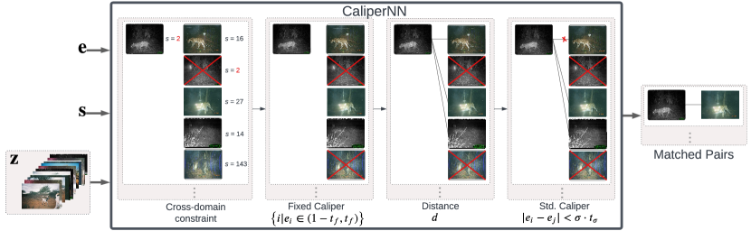
For the matching component of our algorithm, we propose to use a variant of -NN which, in addition to incorporating the above cross-domain constraint, filters the queries and keys that represent probable outliers, according to their learned propensity scores. The initial stage of filtering employs a fixed caliper, where samples with propensity scores surpassing a fixed confidence threshold are removed; this is followed by a second stage of filtering wherein any two samples (from different domains) can only be matched if the Euclidean distance between their respective propensity scores is below a pre-defined threshold (std-caliper). See Fig 1 for a pictorial representation of these steps and Appendix G for reference pseudocode.
The propensity score, , for a given sample is estimated as using a linear classifier , where is the probability simplex over possible domain labels, . is trained via maximum (weighted) likelihood to predict the domain label of a given sample for all samples within the aggregate dataset , or (typically) a subset of it, encoded by . Since we apply both calipers to the learned propensity score, the shape of this distribution can have a significant effect on the outcome of matching. Accordingly, we apply temperature-scaling, with scalar , to sharpen or flatten the learned propensity-score distribution such that we have . We denote the set of associated parameters ({ , as the threshold for the fixed-caliper, the threshold for the std-caliper, and the temperature, respectively) as and discuss in Appendix D how one can determine suitable values for these in practice.
For convenience we define the set of all encodings, given by , as , the set of all associated propensity scores as , and the set of associated domain labels as . In the offline case, the matches for are then computed as
| (4) |
with \CNN returning the set of -nearest neighbours according to , subject to the aforementioned cross-domain and caliper-based constraints. We allow for the fact that there may be no valid matches for some samples due to these constraints; in such cases we have as the second element of their tuples, indicating that should be set to .
3.3 Scaling up with Online Learning
Re-encoding the dataset following each update of the feature-extractor, in order to recompute , is prohibitively expensive, with cost scaling linearly with . Moreover, \CNN requires explicit computation of the pairwise distance matrices, which can be prohibitive memory-wise for large values of . We address these problems using a fixed-size memory bank, storing only the last (where ) encodings from a slow-moving momentum encoder [30, 33], , which we refer to as the target encoder, in line with [30], and accordingly refer to as the online encoder. Unlike [30], however, we make use of neither a projector nor a predictor head (in the case of the target encoder) in order to compute the inputs to the consistency loss and simply use the output of the backbone as is – this is possible in our setting due to preventing representational collapse. More specifically, the target encoder’s parameters, , are computed as a moving average of the online encoder’s, , with decay rate , per the recurrence relation
| (5) |
As the associated domain labels are also needed both for matching and to compute the loss for the propensity scorer, we also store the labels associated with in a companion memory bank . We initialise and to , resulting in fewer than samples being used during the initial stages of training when the memory banks are yet to be populated.
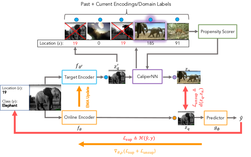
Each iteration of training, we sample a batch of size from consisting of inputs and . During the matching phase, the inputs are passed through the target encoder to obtain , serving as the queries for \CNN. We also experiment with a simpler variant where the online encoder is instead used for this query-generation step, such that we instead have , and find this can work equally well if is sufficiently high. The keys are then formed by combining the current queries with the past queries contained in the memory bank: . The domain labels associated with are likewise formed by concatenating the domain labels in the current batch with those stored in : . Once the matches for the current samples have been computed, the oldest samples in and are overwritten with and , respectively. The consistency loss is then enforced between each query , according to the differentiable online encoder, and each of its matches, providing that (that is, under the condition that the estimated propensity score for does not violate the caliper(s) and there are at least valid matches whose estimated propensity scores also do not), with the loss simply otherwise. Since is frozen, carries an implicit stop-gradient and gradients are computed only w.r.t. . These steps are illustrated pictorially in Fig 2 and as pseudocode in Appendix G.
Similarly, rather than solving for the optimal parameters, for the propensity scorer given the current values of , which is infeasible for the large values of needed to well-approximate the full dataset, we resort to a biased estimate of . Namely, we train in an online fashion to minimise the per-batch loss
| (6) |
where is the standard cross-entropy loss between the predictive distribution and the (degenerate) ground-truth distribution, given by the one-hot encoded domain labels, and is a function assigning to each an importance weight [66] based on the inverse of its frequency in to counteract label imbalance. In the special case in which the and are known to have disjoint support over (that is, ), we can substitute their domain labels with and , respectively (such that we have and ), thus reducing the propensity scorer and \CNN to their binary forms. Knowing whether this condition is satisfied a priori (and thus whether the use of domain labels can be forgone completely from our pipeline) is not unrealistic: one may, for example know that two sets of satellite imagery cover two different parts of the world (e.g. Africa and Asia) yet not know the exact coordinates underlying their respective coverage.
4 Related Work
Domain Generalisation
The goal of domain generalisation (DG) is to produce models that are robust to a wide range of distribution shifts (including those outside the training distribution), given a training set consisting of samples sourced from multiple domains. Despite the various techniques (many well theoretically-motivated) designed to improve the generalisation of deep neural networks current methods continue to fall short in the face of natural distribution shifts [31, 41]. Indeed, ERM has repeatedly shown to be a strong baseline – frequently outperforming dedicated methods that leverage domain information or additional unlabelled data – for DG [31, 63], despite the theoretical problems associated with using it when the training and test sets are misaligned. Until now, only pre-training on larger, more diverse datasets (with harder examples), has consistently proven to improve OOD generalisation, yet allowing pre-trained models to fit the ID data too closely can undo any such benefit conferred by the pre-training [3, 39, 69, 74]. Similar to Okapi, MatchDG [51] draws upon causal matching to tackle DG. Despite the surface-level similarity, there are a number of significant differences, principally in the respects that we consider semi-supervised DG (whereas MatchDG requires full-labeling w.r.t. ) and employ an augmented form of k-NN for bias-reduction in the absence of .
Self-Supervised Learning
In self-supervised learning (SelfSL), models are trained to solve pretext tasks constructed from the input data. This learning paradigm has led to significant breakthroughs in unsupervised learning in recent years, with performance now approaching (or even surpassing, along some axes such as adversarial robustness) that of supervised methods for many tasks while requiring significantly less labelled data. Due to its generality, SelfSL has seen use across the complete spectrum of applications and modalities and underlies many of the foundation models [11] that have emerged in NLP [13, 16, 21], Computer Vision [29], and at their intersection [2, 78]. Common pretext tasks include those based on the masked-language-modelling approach – originally popularised by BERT [21] and recently generalised to other modalities [6, 7] – [15, 33], contrastive captioning [56, 78], and instance discrimination and self-distillation [14, 30] which rely on transformations of the data to generate multi-view inputs. Approaches belonging to the latter two categories were originally limited by the fact that the transforms had to be tailored for a particular modality and for some modalities, such as tabular data, there is no obvious way to define them. A number of recent works have sought to obviate this problem through the use of MixUp [72], masking [6, 34], and k-NN [24, 42, 71], the latter of which is directly relevant to our work. Okapi bears closest resemblance to [42] in combining momentum-encoding with nearest-neighbours lookup to generate the views for a BYOL-style [30] consistency loss. However, a key distinction lies in the use of an augmented form of nearest-neighbours, \CNN, which both constrains pairs of samples to being from different domains and filters out any queries or keys deemed outliers according to a learned propensity score.
Semi-Supervised Learning
Semi-supervised learning (SemiSL) encompasses a broad class of algorithms that combine unsupervised learning with supervised learning in order to improve the performance of the latter, especially when labelled data is limited. Many SemiSL methods are based on the self-training paradigm which can trace its roots back decades to the early work in pattern recognition by [65] and continues to be relevant in the modern era due to its generality, both within SemiSL itself and in related fields such as domain adaptation [27], and fledgling field of SelfSL [14] discussed above. Self-training applies to any framework predicated on using a model’s own predictions to produce pseudo-labels for the unlabelled data which can either be used as targets for self-distillation [75] or enforcing consistency between predictions that themselves have been perturbed [5, 75] or that have been generated from perturbed/multi-view inputs [67]. FixMatch [67] is one example of a consistency-based method which has proven effective for semi-supervised classification, despite its simplicity, and various works [28, 46] have since built on the its framework prescribing the use of weakly- and strongly-augmented inputs to generate the targets and predictions, respectively. Like these methods, Okapi also makes use of a cross-view consistency loss, however, the alternative views for a given sample are generated not through data-augmentation but through statistical matching [58], with the aim being to achieve invariance to the domain rather than a particular series of perturbations. Another example of particular relevance to our work is [70], which uses a copy of the model with exponentially-averaged weights to generate the targets for the unlabelled data. Okapi also uses such a model to produce the targets for its consistency loss, but is more akin to momentum-encoding [33] in the respect that the loss is imposed on the latent space.
5 Experiments
5.1 Datasets
We evaluate Okapi on three datasets taken from the WILDS 2.0 benchmark [63]. These span a variety of modalities and tasks, allowing us to showcase the generality of our proposed method (Okapi): iWildCam (images, multiclass classification), PovertyMap (multispectral images, regression), and CivilComments (text, binary classification). Details of each dataset can be found in Appendix A.
5.2 Image experiments
| Method | iWildCam | PovertyMap | ||||
| macro F1 | worst U/R corr. | worst U/R MSE | ||||
| ID | OOD | ID | OOD | ID | OOD | |
| ERM [63] | 47.0 (1.4) | 32.2 (1.2) | 0.66 (0.04) | 0.49 (0.06) | - | - |
| FixMatch [63] | 46.3 (0.5) | 31.0 (1.3) | 0.54 (0.10) | 0.30 (0.11) | - | - |
| ERM | 48.6 (1.1) | 33.3 (0.3) | 0.72 (0.03) | 0.53 (0.09) | 0.23 (0.03) | 0.35 (0.12) |
| FixMatch | 51.1 (1.0) | 35.2 (0.7) | 0.50 (0.13) | 0.34 (0.12) | 0.59 (0.42) | 0.88 (0.61) |
| Okapi (ours) | 50.6 (0.7) | 36.1 (0.9) | 0.72 (0.02) | 0.55 (0.10) | 0.22 (0.02) | 0.33 (0.10) |
| Okapi (no calipers) | - | - | 0.72 (0.02) | 0.54 (0.12) | 0.22 (0.02) | 0.36 (0.14) |
Results of our image-data experiments are summarised in Table 1. Due to spacial constraints, we defer the full set of results, including those for the ‘offline’ (w.r.t. the matching) version of Okapi to Appendix. C. For both datasets in question, we use the same metrics as [63]: macro-F1 for iWildCam and worst-group (with the group defined as urban (U) vs. rural (R)) Pearson correlation for Poverty Map. For completeness, we include mean squared error (MSE) as a secondary metric for the latter dataset. Following [63], we compute the mean and standard deviation (shown in parentheses) over multiple runs for both ID and OOD test sets, with these runs conducted with 3 different random seeds and 5 pre-defined cross-validation folds for iWildCam and PovertyMap, respectively.
We compare Okapi against two baselines, ERM and FixMatch [67], both according to our re-implementation and according to the original implementation given in [63]. We note that since FixMatch, in its original form, is only applicable to classification problems due to its use of confidence-based thresholding, for the PovertyMap dataset, FixMatch represents a simplified variant (following [63]) without such thresholding, that is trained to simply minimise the MSE between all regressed values for the weakly- and strongly-augmented images. As described in Appendix D, the main difference between the baselines run included in [63] and our re-runs is in the backbone architecture, with us opting for a ConvNeXt [47] architecture over a ResNet one. For both datasets, and for both baselines we observe significant improvements stemming the change of backbone. Moreover, utilising ConvNeXt seems to be crucial in enabling FixMatch to surpass the ERM baseline in the classification task with (ERM) vs (FixMatch) and (ERM) vs. (FixMatch), with ResNet and ConvNeXt architecture respectively.
Okapi, convincingly outperforms the baselines, w.r.t the OOD metric of interest, on both datasets. We observe an improvement of macro F1, i.e. vs of Okapi and FixMatch (the best baseline for iWildCam) respectively. For the regression task in PovertyMap, Okapi achieves and on the OOD test set in terms of Pearson correlation and MSE, respectively, in contrast to the and of ERM. At the same time, we note that FixMatch fails to generalise well to this task, yielding by far the worst results amongst the evaluated methods.
5.3 Text classification
In Table 2 we summarise the numerical results for the CivilComments dataset. Remaining consistent with [63], we evaluate models according to the worst-group accuracy – the minimum of the conditional accuracies obtained by conditioning on each of the 8 dimensions of – averaged over 5 replicates. Since there is no canonical ID test split available for this dataset, we report only the results only for the OOD split that is, rather than doing so for a custom split to avoid misrepresentation. We compare Okapi against both ERM variants featured in [63] – one trained on only the official labelled data and one trained with annotated unlabelled data (fully-labelled) – as well as our re-implementation of the ERM variant trained on only the labelled data with an identical hyperparameter configuration to the former. In contrast to the image datasets, we do not diverge in our choice of architecture, with all models trained with a pre-trained DistilBERT [64] backbone.
We observe marked improvement in the worst-group accuracy of this baseline compared with that reported therein. We attribute this partly to the high variance of the model-selection procedure (inherited from [63]) based on intermittently-computed validation performance (which does not consistently align with test performance) to determine the final model. This aside, we observe that Okapi outperforms the ERM baseline by a significant margin, to the point of parity with the fully-labelled baseline.
5.4 Ablations and qualitatitive analysis
In order to evaluate the importance of the caliper-based filtering to the performance of Okapi, we perform an ablation experiment on PovertyMap dataset (Okapi (no calipers)) with said filtering disabled (and all else constant), such that instead of \CNN we have standard -NN, albeit with the cross-group constraint still in place (per Eq. 2). We see that performance degrades according to both metrics of interest, and, crucially, that the standard deviation of the runs is significantly higher, in line with our expectation that filtering out poor matches should stabilise optimisation. We provide additional ablation experiments in Appendix F, exploring the relative importance of the two (fixed and std-) calipers, the optimal number of neighbours to use for computing , and the feasibility of using the online encoder to generate the queries for \CNN.
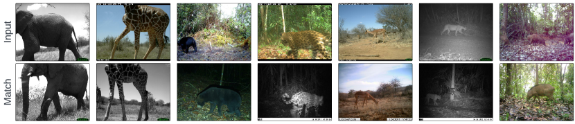
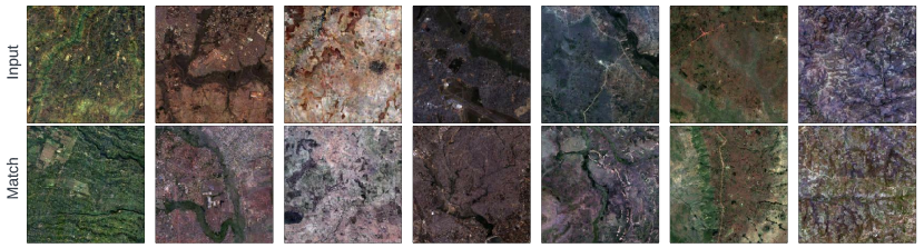
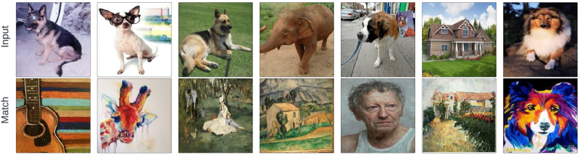
Finally, in Fig. 3 we show samples of matched pairs retrieved by \CNN from the encodings of the learned encoder for the iWildCam dataset. Here, we see that semantic information (encoding the species of animal) is preserved across pairs, while nuisance factors such as illumination, background and contrast vary. Further examples from PovertyMap are shown in Appendix E. In Appendix H, we include matching results for the PACS (photo (P), art painting (A), cartoon (C), and sketch (S)) dataset [45] demonstrating how temperature scaling, in conjunction with the fixed caliper, can be used to control the filtering rate.
6 Conclusion
In this work, we introduced, Okapi, a semi-supervised method for training distributionally-robust models that is intuitive, effective, and is applicable to any modality or task. Okapi is based on the simple idea of supplementing the supervised loss with a cross-domain consistency loss that encourages the outputs of an encoder network to be similar for neighbouring (within the latent space of the encoder itself) samples belonging to different domains, which is made efficient using an online-learning framework. Rather than simply using -NN with a cross-domain constraint, however, we propose an augmented form based on statistical matching (\CNN) that combines propensity scores with calipers to winnow out low-quality matches; we find this to be important for both the end-performance and consistency of Okapi. Our work serves as a response to [63], in that we find that it is in fact possible to effectively incorporate unlabelled data and domain information into a training algorithm in order to improve upon ERM with respect to an OOD test set, assuming an appropriate choice of architecture. Namely, on three datasets from the WILDS 2.0 benchmark, representing two different tasks (classification and regression) and modalities (image and text), we show that Okapi outperforms both the ERM and FixMatch baselines according to the relevant OOD metrics.
Buoyed by these promising results, we intend to apply Okapi to other tasks (e.g. object detection and image segmentation) and other modalities (e.g. audio) to further establish its generality. Furthermore, one limitation of the current incarnation of the method is that the thresholds for the calipers are fixed over the course of training whereas it may be beneficial to set these adaptively with the view to optimise such measures of inter-domain balance as Variance Ratio and Standard Mean Differences that are commonly used to evaluate the the goodness of statistical matching procedures.
Acknowledgments and Disclosure of Funding
This research was supported by a European Research Council (ERC) Starting Grant for the project "Bayesian Models and Algorithms for Fairness and Transparency", funded under the European Union’s Horizon 2020 Framework Programme (grant agreement no. 851538). NQ is also supported by the Basque Government through the BERC 2018-2021 program and by Spanish Ministry of Sciences, Innovation and Universities: BCAM Severo Ochoa accreditation SEV-2017-0718.
References
- Agarwal et al. [2018] A. Agarwal, A. Beygelzimer, M. Dudík, J. Langford, and H. Wallach. A reductions approach to fair classification. In International Conference on Machine Learning, pages 60–69. PMLR, 2018.
- Alayrac et al. [2022] J.-B. Alayrac, J. Donahue, P. Luc, A. Miech, I. Barr, Y. Hasson, K. Lenc, A. Mensch, K. Millican, M. Reynolds, et al. Flamingo: a visual language model for few-shot learning. arXiv preprint arXiv:2204.14198, 2022.
- Andreassen et al. [2021] A. Andreassen, Y. Bahri, B. Neyshabur, and R. Roelofs. The evolution of out-of-distribution robustness throughout fine-tuning. arXiv preprint arXiv:2106.15831, 2021.
- Arjovsky et al. [2019] M. Arjovsky, L. Bottou, I. Gulrajani, and D. Lopez-Paz. Invariant risk minimization. arXiv preprint arXiv:1907.02893, 2019.
- Bachman et al. [2014] P. Bachman, O. Alsharif, and D. Precup. Learning with pseudo-ensembles. Advances in neural information processing systems, 27, 2014.
- Baevski et al. [2022] A. Baevski, W.-N. Hsu, Q. Xu, A. Babu, J. Gu, and M. Auli. Data2vec: A general framework for self-supervised learning in speech, vision and language. arXiv preprint arXiv:2202.03555, 2022.
- Bao et al. [2021] H. Bao, L. Dong, and F. Wei. Beit: Bert pre-training of image transformers. arXiv preprint arXiv:2106.08254, 2021.
- Beery et al. [2020] S. Beery, E. Cole, and A. Gjoka. The iwildcam 2020 competition dataset. arXiv preprint arXiv:2004.10340, 2020.
- Berthet et al. [2020] Q. Berthet, M. Blondel, O. Teboul, M. Cuturi, J.-P. Vert, and F. Bach. Learning with differentiable pertubed optimizers. Advances in neural information processing systems, 33:9508–9519, 2020.
- Biglan et al. [2000] A. Biglan, D. Ary, and A. C. Wagenaar. The value of interrupted time-series experiments for community intervention research. Prevention Science, 1(1):31–49, 2000.
- Bommasani et al. [2021] R. Bommasani, D. A. Hudson, E. Adeli, R. Altman, S. Arora, S. von Arx, M. S. Bernstein, J. Bohg, A. Bosselut, E. Brunskill, et al. On the opportunities and risks of foundation models. arXiv preprint arXiv:2108.07258, 2021.
- Borkan et al. [2019] D. Borkan, L. Dixon, J. Sorensen, N. Thain, and L. Vasserman. Nuanced metrics for measuring unintended bias with real data for text classification. In Companion proceedings of the 2019 world wide web conference, pages 491–500, 2019.
- Brown et al. [2020] T. Brown, B. Mann, N. Ryder, M. Subbiah, J. D. Kaplan, P. Dhariwal, A. Neelakantan, P. Shyam, G. Sastry, A. Askell, et al. Language models are few-shot learners. Advances in neural information processing systems, 33:1877–1901, 2020.
- Caron et al. [2021] M. Caron, H. Touvron, I. Misra, H. Jégou, J. Mairal, P. Bojanowski, and A. Joulin. Emerging properties in self-supervised vision transformers. In Proceedings of the IEEE/CVF International Conference on Computer Vision, pages 9650–9660, 2021.
- Chen et al. [2020] T. Chen, S. Kornblith, M. Norouzi, and G. Hinton. A simple framework for contrastive learning of visual representations. In International conference on machine learning, pages 1597–1607. PMLR, 2020.
- Chowdhery et al. [2022] A. Chowdhery, S. Narang, J. Devlin, M. Bosma, G. Mishra, A. Roberts, P. Barham, H. W. Chung, C. Sutton, S. Gehrmann, et al. Palm: Scaling language modeling with pathways. arXiv preprint arXiv:2204.02311, 2022.
- Christian et al. [2010] P. Christian, L. E. Murray-Kolb, S. K. Khatry, J. Katz, B. A. Schaefer, P. M. Cole, S. C. LeClerq, and J. M. Tielsch. Prenatal micronutrient supplementation and intellectual and motor function in early school-aged children in nepal. Jama, 304(24):2716–2723, 2010.
- Creager et al. [2019] E. Creager, D. Madras, J.-H. Jacobsen, M. Weis, K. Swersky, T. Pitassi, and R. Zemel. Flexibly fair representation learning by disentanglement. In International conference on machine learning, pages 1436–1445. PMLR, 2019.
- Creager et al. [2021] E. Creager, J.-H. Jacobsen, and R. Zemel. Environment inference for invariant learning. In International Conference on Machine Learning, pages 2189–2200. PMLR, 2021.
- Crump et al. [2009] R. K. Crump, V. J. Hotz, G. W. Imbens, and O. A. Mitnik. Dealing with limited overlap in estimation of average treatment effects. Biometrika, 96(1):187–199, 2009.
- Devlin et al. [2018] J. Devlin, M.-W. Chang, K. Lee, and K. Toutanova. Bert: Pre-training of deep bidirectional transformers for language understanding. arXiv preprint arXiv:1810.04805, 2018.
- Donini et al. [2018] M. Donini, L. Oneto, S. Ben-David, J. S. Shawe-Taylor, and M. Pontil. Empirical risk minimization under fairness constraints. Advances in Neural Information Processing Systems, 31, 2018.
- Dunnmon et al. [2019] J. A. Dunnmon, D. Yi, C. P. Langlotz, C. Ré, D. L. Rubin, and M. P. Lungren. Assessment of convolutional neural networks for automated classification of chest radiographs. Radiology, 290(2):537–544, 2019.
- Dwibedi et al. [2021] D. Dwibedi, Y. Aytar, J. Tompson, P. Sermanet, and A. Zisserman. With a little help from my friends: Nearest-neighbor contrastive learning of visual representations. In Proceedings of the IEEE/CVF International Conference on Computer Vision, pages 9588–9597, 2021.
- Dwork et al. [2012] C. Dwork, M. Hardt, T. Pitassi, O. Reingold, and R. Zemel. Fairness through awareness. In Proceedings of the 3rd innovations in theoretical computer science conference, pages 214–226, 2012.
- Feldman et al. [2015] M. Feldman, S. A. Friedler, J. Moeller, C. Scheidegger, and S. Venkatasubramanian. Certifying and removing disparate impact. In proceedings of the 21th ACM SIGKDD international conference on knowledge discovery and data mining, pages 259–268, 2015.
- Ganin et al. [2016] Y. Ganin, E. Ustinova, H. Ajakan, P. Germain, H. Larochelle, F. Laviolette, M. Marchand, and V. Lempitsky. Domain-adversarial training of neural networks. The journal of machine learning research, 17(1):2096–2030, 2016.
- Gong et al. [2021] C. Gong, D. Wang, and Q. Liu. Alphamatch: Improving consistency for semi-supervised learning with alpha-divergence. In Proceedings of the IEEE/CVF Conference on Computer Vision and Pattern Recognition, pages 13683–13692, 2021.
- Goyal et al. [2022] P. Goyal, Q. Duval, I. Seessel, M. Caron, M. Singh, I. Misra, L. Sagun, A. Joulin, and P. Bojanowski. Vision models are more robust and fair when pretrained on uncurated images without supervision. arXiv preprint arXiv:2202.08360, 2022.
- Grill et al. [2020] J.-B. Grill, F. Strub, F. Altché, C. Tallec, P. Richemond, E. Buchatskaya, C. Doersch, B. Avila Pires, Z. Guo, M. Gheshlaghi Azar, et al. Bootstrap your own latent-a new approach to self-supervised learning. Advances in Neural Information Processing Systems, 33:21271–21284, 2020.
- Gulrajani and Lopez-Paz [2020] I. Gulrajani and D. Lopez-Paz. In search of lost domain generalization. In International Conference on Learning Representations, 2020.
- Hardt et al. [2016] M. Hardt, E. Price, and N. Srebro. Equality of opportunity in supervised learning. Advances in neural information processing systems, 29, 2016.
- He et al. [2020] K. He, H. Fan, Y. Wu, S. Xie, and R. Girshick. Momentum contrast for unsupervised visual representation learning. In Proceedings of the IEEE/CVF conference on computer vision and pattern recognition, pages 9729–9738, 2020.
- He et al. [2021] K. He, X. Chen, S. Xie, Y. Li, P. Dollár, and R. Girshick. Masked autoencoders are scalable vision learners. arXiv:2111.06377, 2021.
- Hurley and Adebayo [2017] M. Hurley and J. Adebayo. Credit scoring in the era of big data. Yale Journal of Law and Technology, 18:148–216, 2017.
- Idrissi et al. [2022] B. Y. Idrissi, M. Arjovsky, M. Pezeshki, and D. Lopez-Paz. Simple data balancing achieves competitive worst-group-accuracy. In Conference on Causal Learning and Reasoning, pages 336–351. PMLR, 2022.
- Kamiran and Calders [2012] F. Kamiran and T. Calders. Data preprocessing techniques for classification without discrimination. Knowledge and information systems, 33(1):1–33, 2012.
- Kehrenberg et al. [2020] T. Kehrenberg, M. Bartlett, O. Thomas, and N. Quadrianto. Null-sampling for interpretable and fair representations. In European Conference on Computer Vision, pages 565–580. Springer, 2020.
- Kim et al. [2022] D. Kim, K. Wang, S. Sclaroff, and K. Saenko. A broad study of pre-training for domain generalization and adaptation. arXiv preprint arXiv:2203.11819, 2022.
- King and Nielsen [2019] G. King and R. Nielsen. Why propensity scores should not be used for matching. Political Analysis, 27(4):435–454, 2019.
- Koh et al. [2021] P. W. Koh, S. Sagawa, H. Marklund, S. M. Xie, M. Zhang, A. Balsubramani, W. Hu, M. Yasunaga, R. L. Phillips, I. Gao, et al. Wilds: A benchmark of in-the-wild distribution shifts. In International Conference on Machine Learning, pages 5637–5664. PMLR, 2021.
- Koohpayegani et al. [2021] S. A. Koohpayegani, A. Tejankar, and H. Pirsiavash. Mean shift for self-supervised learning. In Proceedings of the IEEE/CVF International Conference on Computer Vision, pages 10326–10335, 2021.
- Krueger et al. [2021] D. Krueger, E. Caballero, J.-H. Jacobsen, A. Zhang, J. Binas, D. Zhang, R. Le Priol, and A. Courville. Out-of-distribution generalization via risk extrapolation (rex). In International Conference on Machine Learning, pages 5815–5826. PMLR, 2021.
- Lahoti et al. [2019] P. Lahoti, K. Gummadi, and G. Weikum. Operationalizing individual fairness with pairwise fair representations. Proceedings of the VLDB Endowment, 13(4):506–518, 2019.
- Li et al. [2017] D. Li, Y. Yang, Y.-Z. Song, and T. M. Hospedales. Deeper, broader and artier domain generalization. In Proceedings of the IEEE international conference on computer vision, pages 5542–5550, 2017.
- Lienen and Hüllermeier [2021] J. Lienen and E. Hüllermeier. Credal self-supervised learning. In M. Ranzato, A. Beygelzimer, Y. Dauphin, P. Liang, and J. W. Vaughan, editors, Advances in Neural Information Processing Systems, volume 34, pages 14370–14382. Curran Associates, Inc., 2021. URL https://proceedings.neurips.cc/paper/2021/file/7866c91c59f8bffc92a79a7cd09f9af9-Paper.pdf.
- Liu et al. [2022] Z. Liu, H. Mao, C.-Y. Wu, C. Feichtenhofer, T. Darrell, and S. Xie. A convnet for the 2020s. arXiv preprint arXiv:2201.03545, 2022.
- Loshchilov and Hutter [2017] I. Loshchilov and F. Hutter. SGDR: stochastic gradient descent with warm restarts. In 5th International Conference on Learning Representations, ICLR 2017, Toulon, France, April 24-26, 2017, Conference Track Proceedings. OpenReview.net, 2017. URL https://openreview.net/forum?id=Skq89Scxx.
- Loshchilov and Hutter [2018] I. Loshchilov and F. Hutter. Decoupled weight decay regularization. In International Conference on Learning Representations, 2018.
- Madras et al. [2018] D. Madras, E. Creager, T. Pitassi, and R. Zemel. Learning adversarially fair and transferable representations. In International Conference on Machine Learning, pages 3384–3393. PMLR, 2018.
- Mahajan et al. [2021] D. Mahajan, S. Tople, and A. Sharma. Domain generalization using causal matching. In International Conference on Machine Learning, pages 7313–7324. PMLR, 2021.
- Muandet et al. [2013] K. Muandet, D. Balduzzi, and B. Schölkopf. Domain generalization via invariant feature representation. In International Conference on Machine Learning, pages 10–18. PMLR, 2013.
- Oneto et al. [2020] L. Oneto, M. Donini, G. Luise, C. Ciliberto, A. Maurer, and M. Pontil. Exploiting mmd and sinkhorn divergences for fair and transferable representation learning. Advances in Neural Information Processing Systems, 33:15360–15370, 2020.
- Paszke et al. [2019] A. Paszke, S. Gross, F. Massa, A. Lerer, J. Bradbury, G. Chanan, T. Killeen, Z. Lin, N. Gimelshein, L. Antiga, et al. Pytorch: An imperative style, high-performance deep learning library. Advances in neural information processing systems, 32, 2019.
- Quadrianto et al. [2019] N. Quadrianto, V. Sharmanska, and O. Thomas. Discovering fair representations in the data domain. In Proceedings of the IEEE/CVF conference on computer vision and pattern recognition, pages 8227–8236, 2019.
- Radford et al. [2021] A. Radford, J. W. Kim, C. Hallacy, A. Ramesh, G. Goh, S. Agarwal, G. Sastry, A. Askell, P. Mishkin, J. Clark, et al. Learning transferable visual models from natural language supervision. In International Conference on Machine Learning, pages 8748–8763. PMLR, 2021.
- Romiti et al. [2022] S. Romiti, C. Inskip, V. Sharmanska, and N. Quadrianto. Realpatch: A statistical matching framework for model patching with real samples. CoRR, abs/2208.02192, 2022.
- Rosenbaum and Rubin [1983] P. R. Rosenbaum and D. B. Rubin. The central role of the propensity score in observational studies for causal effects. Biometrika, 70(1):41–55, 1983.
- Rosenbaum and Rubin [1985] P. R. Rosenbaum and D. B. Rubin. Constructing a control group using multivariate matched sampling methods that incorporate the propensity score. The American Statistician, 39(1):33–38, 1985.
- Rubin [1973] D. B. Rubin. Matching to remove bias in observational studies. Biometrics, pages 159–183, 1973.
- Rubin [2001] D. B. Rubin. Using propensity scores to help design observational studies: application to the tobacco litigation. Health Services and Outcomes Research Methodology, 2(3):169–188, 2001.
- Sagawa et al. [2019] S. Sagawa, P. W. Koh, T. B. Hashimoto, and P. Liang. Distributionally robust neural networks for group shifts: On the importance of regularization for worst-case generalization. arXiv preprint arXiv:1911.08731, 2019.
- Sagawa et al. [2022] S. Sagawa, P. W. Koh, T. Lee, I. Gao, S. M. Xie, K. Shen, A. Kumar, W. Hu, M. Yasunaga, H. Marklund, S. Beery, E. David, I. Stavness, W. Guo, J. Leskovec, K. Saenko, T. Hashimoto, S. Levine, C. Finn, and P. Liang. Extending the WILDS benchmark for unsupervised adaptation. In International Conference on Learning Representations, 2022. URL https://openreview.net/forum?id=z7p2V6KROOV.
- Sanh et al. [2019] V. Sanh, L. Debut, J. Chaumond, and T. Wolf. Distilbert, a distilled version of bert: smaller, faster, cheaper and lighter. arXiv preprint arXiv:1910.01108, 2019.
- Scudder [1965] H. Scudder. Probability of error of some adaptive pattern-recognition machines. IEEE Transactions on Information Theory, 11(3):363–371, 1965.
- Shimodaira [2000] H. Shimodaira. Improving predictive inference under covariate shift by weighting the log-likelihood function. Journal of statistical planning and inference, 90(2):227–244, 2000.
- Sohn et al. [2020] K. Sohn, D. Berthelot, N. Carlini, Z. Zhang, H. Zhang, C. A. Raffel, E. D. Cubuk, A. Kurakin, and C.-L. Li. Fixmatch: Simplifying semi-supervised learning with consistency and confidence. Advances in Neural Information Processing Systems, 33:596–608, 2020.
- Stuart [2010] E. A. Stuart. Matching methods for causal inference: A review and a look forward. Stat Sci, 25(1):1–21, 2010. ISSN 0883-4237.
- Taori et al. [2020] R. Taori, A. Dave, V. Shankar, N. Carlini, B. Recht, and L. Schmidt. Measuring robustness to natural distribution shifts in image classification. Advances in Neural Information Processing Systems, 33:18583–18599, 2020.
- Tarvainen and Valpola [2017] A. Tarvainen and H. Valpola. Mean teachers are better role models: Weight-averaged consistency targets improve semi-supervised deep learning results. Advances in neural information processing systems, 30, 2017.
- Van Gansbeke et al. [2021] W. Van Gansbeke, S. Vandenhende, S. Georgoulis, and L. V. Gool. Revisiting contrastive methods for unsupervised learning of visual representations. Advances in Neural Information Processing Systems, 34, 2021.
- Verma et al. [2021] V. Verma, T. Luong, K. Kawaguchi, H. Pham, and Q. Le. Towards domain-agnostic contrastive learning. In International Conference on Machine Learning, pages 10530–10541. PMLR, 2021.
- Watson et al. [2019] D. S. Watson, J. Krutzinna, I. N. Bruce, C. E. Griffiths, I. B. McInnes, M. R. Barnes, and L. Floridi. Clinical applications of machine learning algorithms: beyond the black box. Bmj, 364, 2019.
- Wiles et al. [2022] O. Wiles, S. Gowal, F. Stimberg, S.-A. Rebuffi, I. Ktena, K. D. Dvijotham, and A. T. Cemgil. A fine-grained analysis on distribution shift. In International Conference on Learning Representations, 2022. URL https://openreview.net/forum?id=Dl4LetuLdyK.
- Xie et al. [2020] Q. Xie, M.-T. Luong, E. Hovy, and Q. V. Le. Self-training with noisy student improves imagenet classification. In Proceedings of the IEEE/CVF conference on computer vision and pattern recognition, pages 10687–10698, 2020.
- Yeh et al. [2020] C. Yeh, A. Perez, A. Driscoll, G. Azzari, Z. Tang, D. Lobell, S. Ermon, and M. Burke. Using publicly available satellite imagery and deep learning to understand economic well-being in africa. Nature communications, 11(1):1–11, 2020.
- Yu et al. [2020] F. Yu, H. Chen, X. Wang, W. Xian, Y. Chen, F. Liu, V. Madhavan, and T. Darrell. Bdd100k: A diverse driving dataset for heterogeneous multitask learning. In Proceedings of the IEEE/CVF conference on computer vision and pattern recognition, pages 2636–2645, 2020.
- Yu et al. [2022] J. Yu, Z. Wang, V. Vasudevan, L. Yeung, M. Seyedhosseini, and Y. Wu. Coca: Contrastive captioners are image-text foundation models. arXiv preprint arXiv:2205.01917, 2022.
Appendix A Datasets
We evaluate Okapi using three datasets – iWildCam, PovertyMap, and CivilComments – taken from the WILDS 2.0 benchmark [63]. These datasets were chosen specifically due to the poor performance reported by [63] for semi-supervised and domain adaptation methods across the board, in relation to the ERM baselines. For PovertyMap in particular, ERM was found to vastly outperform any competing methods utilising the unlabelled data and/or domain labels.
iWildCam-WILDS is an extension of the iWildCam 2020 Competition Dataset [8]. The task is multi-class species classification of animals in camera trap images. The dataset contains 1022K images of animals annotated with the domain, , that identifies the camera trap that captured it. The target label, , is one of 182 different animal species and it is provided solely for the 203K labelled data. The labelled training set contains 130K images taken by 243 camera traps. The out-of-distribution (OOD) validation and target sets include images from 32 and 48 different camera traps which are disjoint from the 243 training domains. Additionally, 819K unlabelled images from 3215 new domains are available. Different cameras trap differ in characteristics such as illumination, background and relative animal frequency, models trained on the source domains might fail to generalise to images taken from new locations.
PovertyMap-WILDS is a variation of the dataset introduced in [76]. The task is to predict the wealth index, , from multispectral satellite images of 23 African countries. The country the image was taken in as well as whether it was taken in a rural or urban area represent the domain . The dataset contains 5 cross-validation (CV) folds of roughly equal size, each one dividing the 23 countries differently across the source, OOD validation and OOD target splits. In each fold, the labelled training set contains 11K images from 14 different countries. The OOD validation and target sets include images from 5 different countries not represented in the source data. The dataset also includes 261K unlabelled images from the same 23 countries.
CivilComments-WILDS is an online-comment dataset adapted from [12], comprising 448K online comments annotated with both a binary indicator of toxicity () – serving as the target label, – and the demographic identities mentioned within them – serving as the domain . Here, is a binary vector rather than a scalar, with dimensions indicating membership (non-exclusively) to 8 demographic groups, spanning different genders, religions and ethnicities. For the WILDS 2.0 variant of the dataset, [63] introduce an additional corpus of 1551K comments acting as the unlabelled training data belonging to extra domains. While the comments are completely unlabelled, w.r.t. both and and thus are not domain-separable at the sample level, the majority () of the comments are known to be sourced from the same documents as those comments comprising the (OOD) labelled test data. As noted in [63], CivilComments-WILDS exhibits label imbalance w.r.t. ; this is amended both therein and herein (as appertains all methods) through the use of class-balanced sampling, though with the minor distinction that for our experiments we ensure each batch is exactly balanced rather by sampling equally from each class, in contrast to [63] who sample hierarchically – sampling uniformly from and then uniformly from , conditioned on – such that balance is achieved only in expectation.
Appendix B Relation to Algorithmic Fairness
DG and Algorithmic Fairness overlap in their objective to train a model that yields predictions that are statistically independent of (and thus robust to variations in) domain, when for the latter the domain is taken to be some protected characteristic, such as age or gender, and fairness is measured according to invariance-driven notions of group fairness such as Demographic Parity [26] and Equal Opportunity [32]. Indeed, methods that focus on equalising the empirical risk across subgroups – such as by importance weighting [36, 66] – have featured extensively in both DG [4, 19, 43, 62] and fairness [1, 22, 37] and many approaches to fair representation learning [18, 38, 50, 53, 55] have roots in the former [52] and in the closely-related field of domain adaptation [27]. Beyond this more general equivalence, our work also has ties to notions of individual fairness pioneered by [25] – broadly prescribing that similar individuals be treated similarly – in that our unsupervised loss involves maximising the similarity between inter-domain samples within representation space. This is reminiscent of the operationalisation of individual fairness proposed by [44] that enforces similarity between a given representation and the representations of its neighbouring – in both the input space and according to a between-group (cross-domain) quantile graph – samples.
Appendix C Extended Results
We tabulate in Table 3 an extended version of the results presented in the main text. This includes additional results with the ResNet backbones per [63] (justifying our decision to adopt a ConvNext backbone for our main set of image-dataset results) as well as those for an ’offline’ version of Okapi (Okapi (offline)) where the matches are generated prior to training using features of the respective ERM baseline for each dataset. Since the target encoder is necessitated by the need for online match-retrieval, only a single encoder is involved in Okapi (offline); in binary cases, the algorithm is then identical to the one proposed by [57] with the exception that consistency is still enforced via distance in encoding space rather than with a JSD loss on the predictive distributions which fails to generalise to regression tasks such as PovertyMap.
| Method | iWildCam | PovertyMap | ||||
| macro F1 | worst U/R corr. | worst U/R MSE | ||||
| ID | OOD | ID | OOD | ID | OOD | |
| ERM [63] | 47.0 (1.4) | 32.2 (1.2) | 0.66 (0.04) | 0.49 (0.06) | - | - |
| FixMatch [63] | 46.3 (0.50) | 31.0 (1.3) | 0.54 (0.10) | 0.30 (0.11) | - | - |
| ERM (ConvNeXt) | 48.6 (1.1) | 33.3 (0.3) | 0.72 (0.03) | 0.53 (0.09) | 0.23 (0.03) | 0.35 (0.12) |
| FixMatch (ConvNeXt) | 51.1 (1.0) | 35.2 (0.7) | 0.50 (0.13) | 0.34 (0.12) | 0.59 (0.42) | 0.88 (0.61) |
| Okapi (ours; ConvNeXt) | 50.6 (0.7) | 36.1 (0.9) | 0.72 (0.02) | 0.55 (0.10) | 0.22 (0.02) | 0.33 (0.10) |
| Okapi (offline; ConvNeXt) | 48.8 (0.8) | 31.7 (0.2) | 0.68 (0.02) | 0.53 (0.07) | 0.26 (0.02) | 0.37 (0.13) |
| Okapi (no calipers; ConvNeXt) | - | - | 0.72 (0.02) | 0.54 (0.12) | 0.22 (0.02) | 0.36 (0.14) |
| ERM (ResNet) | 46.5 (0.8) | 29.7 (1.0) | 0.69 (0.03) | 0.53 (0.08) | 0.24 (0.04) | 0.34 (0.11) |
| FixMatch (ResNet) | 43.0 (2.5) | 25.5 (1.4) | 0.70 (0.02) | 0.53 (0.08) | 0.24 (0.02) | 0.35 (0.10) |
| Okapi (ResNet) | 46.1 (0.7) | 27.8 (0.3) | 0.70 (0.04) | 0.52 (0.07) | 0.23 (0.02) | 0.33 (0.10) |
Appendix D Implementation details
Data Augmentation
We follow [63] when defining the augmentations for the the WILDS datasets. In the case of PovertyMap-WILDS we corroborate the original finding that data-augmentation adversely affects performance, and, in light of this, elect only to use data-augmentation for FixMatch where it is needed to generate the weak and strong views used in computing the consistency loss. Since Okapi uses an NN-based approach for generating these views, it is decoupled from the augmentation strategy and problems that can arise from its misspecification.
Architecture
For our image experiments, contrary to [63], we opt to use the recently proposed ConvNeXt architecture [47], finding this change to provide large performance gains and to be crucial in enabling semi-supervised methods to surpass the ERM baseline. This is in line with [39] who similarly found that a change of architecture (combined with large-scale pre-training) could greatly bolster performance on the iWildCam dataset. More precisely, we use the tiny variant of ConvNeXt, pre-trained on ImageNet 1k, as the initial backbone for our models. We compose this with a single fully-connected layer to construct the complete predictor both for the target and the propensity score. For our CivilComments experiments, in contrast, we do not diverge from [63] in our choice of architecture, with all models trained with a pre-trained DistilBERT [64].
Optimisation
For optimising all models, we use the AdamW optimiser [49] coupled with a cosine annealing schedule without warm restarts [48]. We set the initial learning to be across the board, and forgo the use of weight decay. Models are trained for K, K, and K iterations for iWildCam, PovertyMap, and CivilComments, respectively. The decay coefficient, , for the target encoder’s exponential moving average is initialised to and is linearly increased to over the course of training. For PovertyMap we set and to be and , respectively; for iWildCam, we set and to be and , respectively, resulting in a fixed value of ; , respectively; for CivilComments, we set and to be and , respectively, again resulting in a fixed value of . We similarly warm up the pre-factor for the consistency loss, , according to a linear schedule during the first of training to allow a period for the encoder to learn meaningful relations between samples through the supervised loss before bootstrapping with the consistency loss, with a final value of .
Matching
In order to determine suitable hyperparameters, , for \CNN, we perform a grid-search in the static setting, using a fixed model. Specifically, we use the backbone of an ERM-trained model as the encoder with which to generate the queries and keys for matching. The quality of matching with a given instantiation of is measured using two metrics commonly used in the statistical matching literature: Variance Ratio (VR) and Standard Mean Differences (SMD) [61]. Both metrics operate on pairs of domains, but can be generalised to work when is non-binary by simply aggregating over all pairwise results. For a given pair of domains, VR is defined as the ratio of the variances of the covariates between the two domains, with an ideal value of , while SMD is defined as the difference in their covariate means, normalised by the standard deviation for each covariate, and is to be minimised. While our proposed method is applicable whether is binary or categorical, for the experiments in this paper we take advantage of the fact that the WILDS datasets specify splits with non-overlapping domains and match from and in the reverse direction (from ). This decision was based on preliminary experiments which found the binary variant generally enjoyed more stable optimisation, something which future work should seek to rectify. In the case of PovertyMap, however, the training splits themselves do not satisfy the aforementioned requirement of being sourced from mutually exclusive sets of domains and we instead treat the OOD validation set as (and treat it as being unlabelled w.r.t. , in that it is only used for ).
Appendix E Additional Matching Examples
Appendix F Ablations
| Method | PovertyMap | |||
| worst U/R corr. | worst U/R MSE | |||
| ID | OOD | ID | OOD | |
| Okapi (k=1) | 0.72 (0.02) | 0.55 (0.10) | 0.22 (0.02) | 0.33 (0.10) |
| Okapi (k=5) | 0.72 (0.02) | 0.55 (0.10) | 0.22 (0.02) | 0.33 (0.10) |
| Okapi (k=10) | 0.72 (0.02) | 0.55 (0.09) | 0.22 (0.02) | 0.33 (0.10) |
| Okapi (k=5, no calipers) | 0.72 (0.02) | 0.54 (0.12) | 0.22 (0.02) | 0.36 (0.14) |
| Okapi (k=5, no std caliper) | 0.72 (0.02) | 0.54 (0.12) | 0.22 (0.02) | 0.35 (0.14) |
| Okapi (k=5, no fixed caliper) | 0.72 (0.02) | 0.55 (0.10) | 0.22 (0.02) | 0.33 (0.10) |
| Method | PovertyMap | |||
| worst U/R corr. | worst U/R MSE | |||
| ID | OOD | ID | OOD | |
| Okapi (TE queries) | 0.72 (0.02) | 0.55 (0.10) | 0.22 (0.02) | 0.33 (0.10) |
| Okapi (OE queries) | 0.72 (0.02) | 0.55 (0.10) | 0.23 (0.02) | 0.34 (0.10) |
We supplement the ablation experiment on the use of calipers featured in the main text with additional experiments concerning effect of the number of nearest neighbours (), the relative importance of the two (fixed and std) calipers, and the feasibility of using the online encoder as the query-generator instead of the target encoder. The results of these experiments are tabulated in 4(b) with the key takeaways being:
-
1.
The number of neighbours used for computing the consistency loss has little impact – according to the given level of precision – on the performance of Okapi along all axes.
-
2.
While disabling the calipers altogether considerably harmed performance, using only the std. caliper allows us to recover the performance of the complete algorithm, (Okapi (k=5)), whereas the same is not true for the fixed caliper which, while aiding performance compared to the no-caliper baseline, falls short of that benchmark. A caveat attached to these conclusions, however, is that the selected values for are likely suboptimal in the online setting, given that they were optimised for the static setting: with improved selection of , either by learning it jointly with the model’s parameters (using, for instance, the perturbed maximum method [9] to overcome the non-differentiability of the -NN and thresholding operations), in an amortised fashion, or optimising it on a per-iteration basis.
-
3.
While less appealing from a conceptual standpoint, due to the mismatch between the networks used to generate the queries and keys, from an empirical standpoint it is perfectly feasible to use the online encoder to generate the queries for statistical matching instead the target encoder while experiencing minimal degradation in performance. This is particularly relevant when one wishes to perform the matching in only one direction (e.g. ) due to the reduction in redundant encoding, with each encoder only encoding its respective subset of the data (e.g. only encodes samples from and only encodes samples from )
Appendix G Pseudocode
We provide Pytorch-style [54] pseudocode for the \CNN (described in 3.2) and online-learning (described in 3.3) algorithms in Algorithm 1 and Algorithm 2, respectively. In both cases, we restrict the pseudocode to the special case of binary domains – practically achieved by using the labelled/unlabelled as a proxy for domain – for ease of illustration. The \CNN algorithm can be generalised freely to multiclass cases by considering pairwise interactions between the propensity scores for each domain for applying the calipers and by computing the pairwise inequalities between and (giving the connectivity matrix , where denotes the ones vector of the same shape as its multiplicand and mediates broadcasting) for enforcing the cross-domain constraint.
Appendix H Matching for PACS dataset
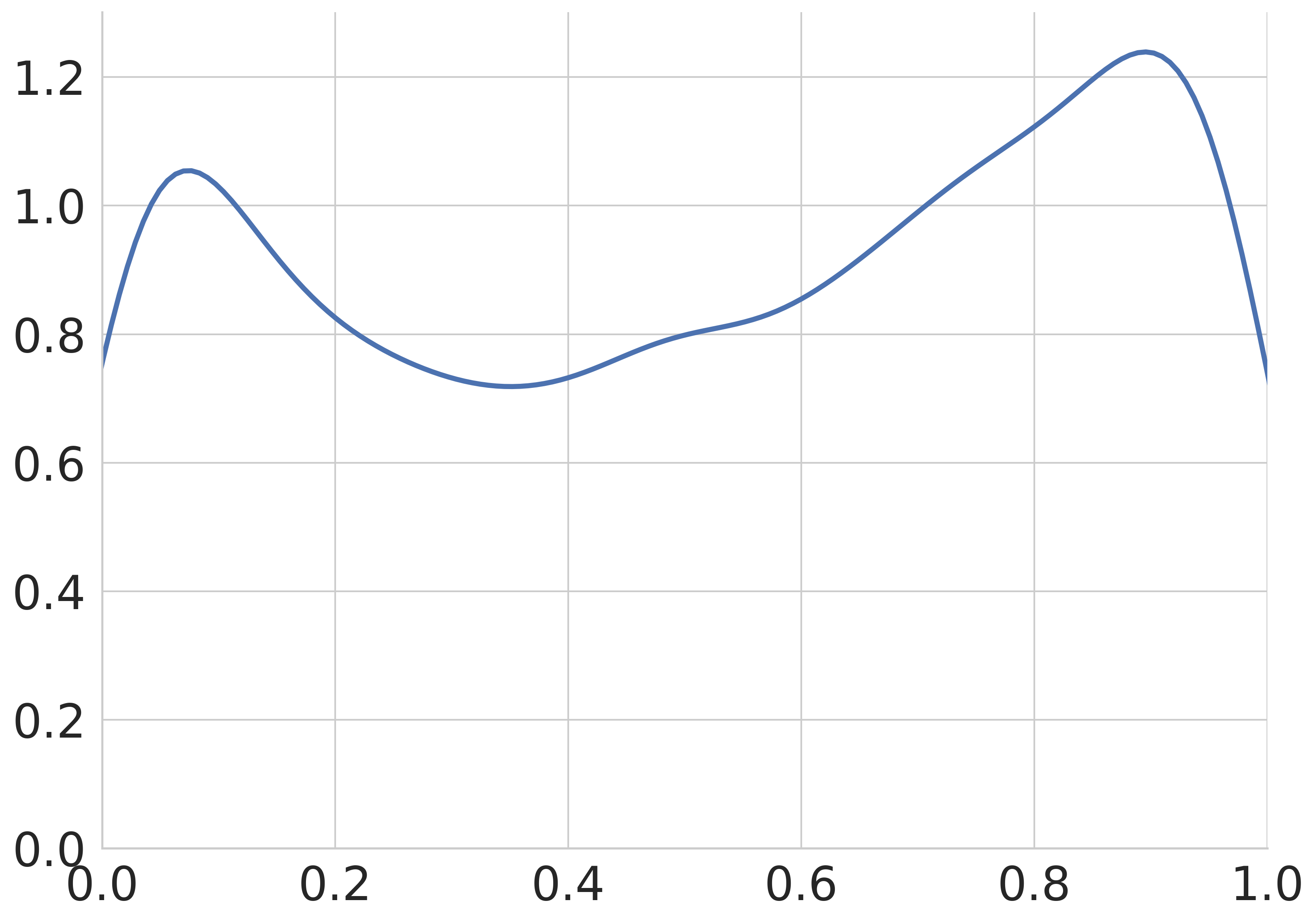
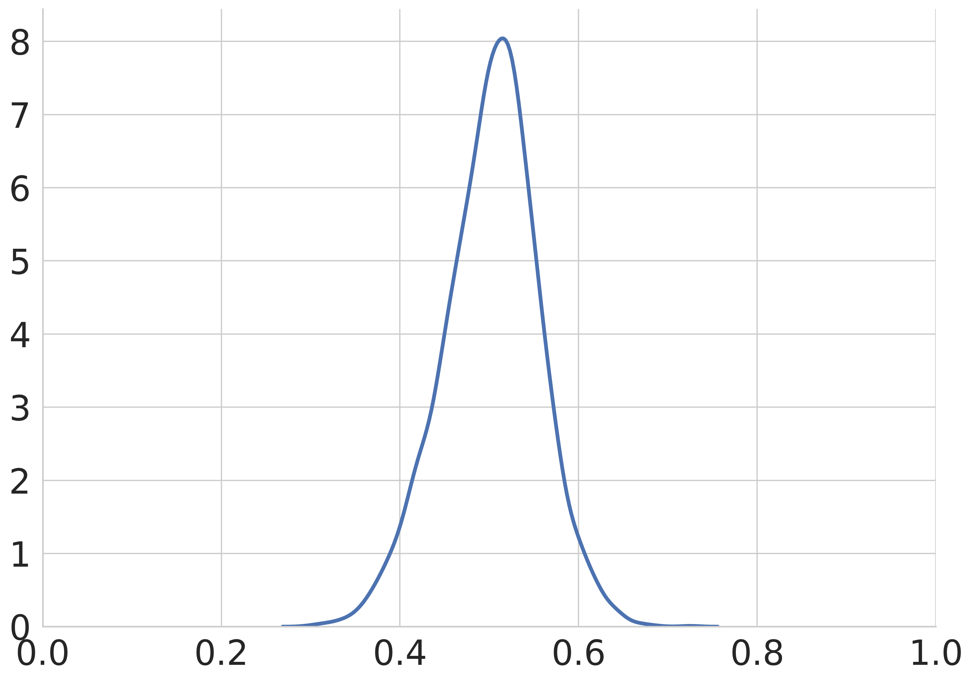
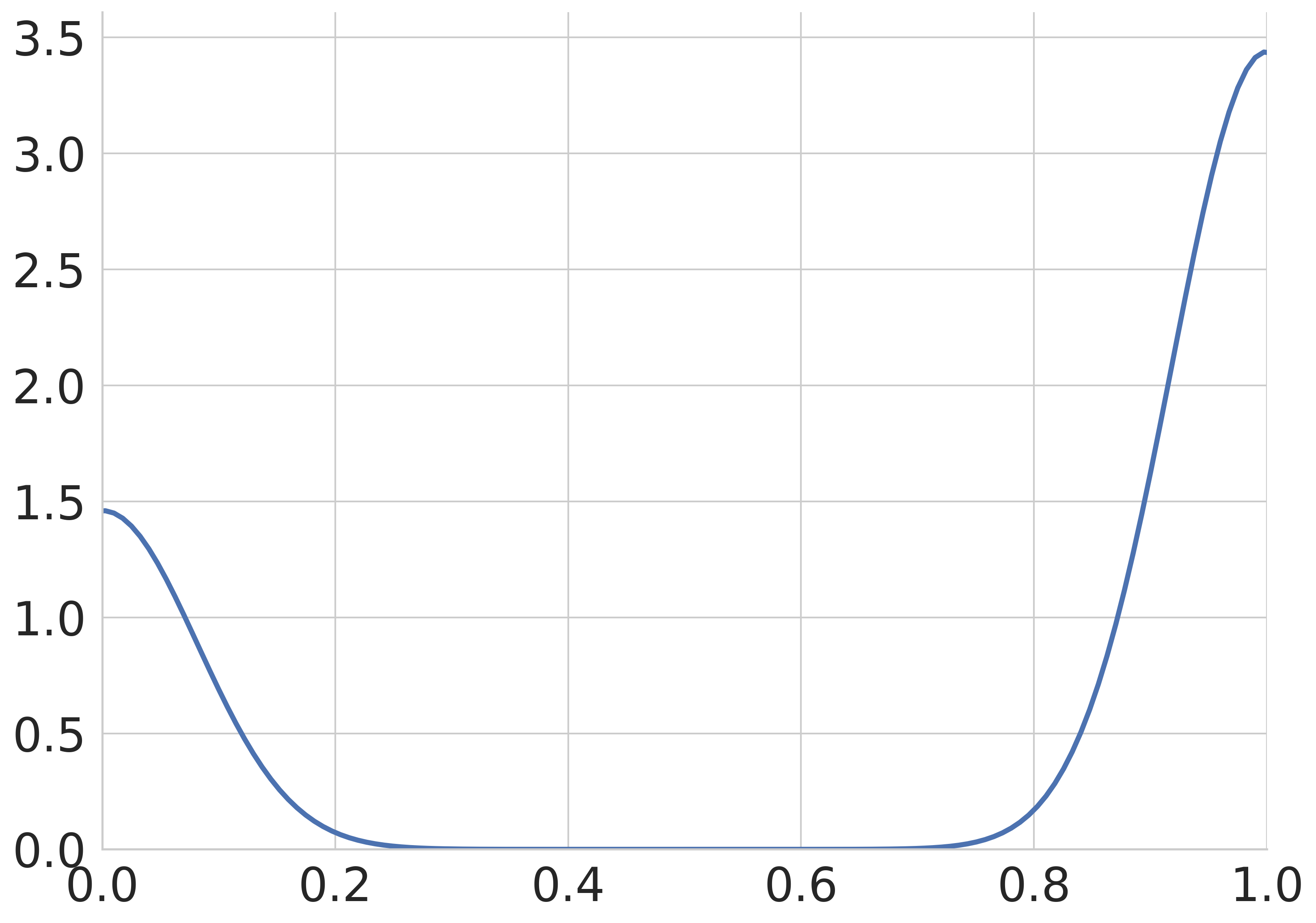
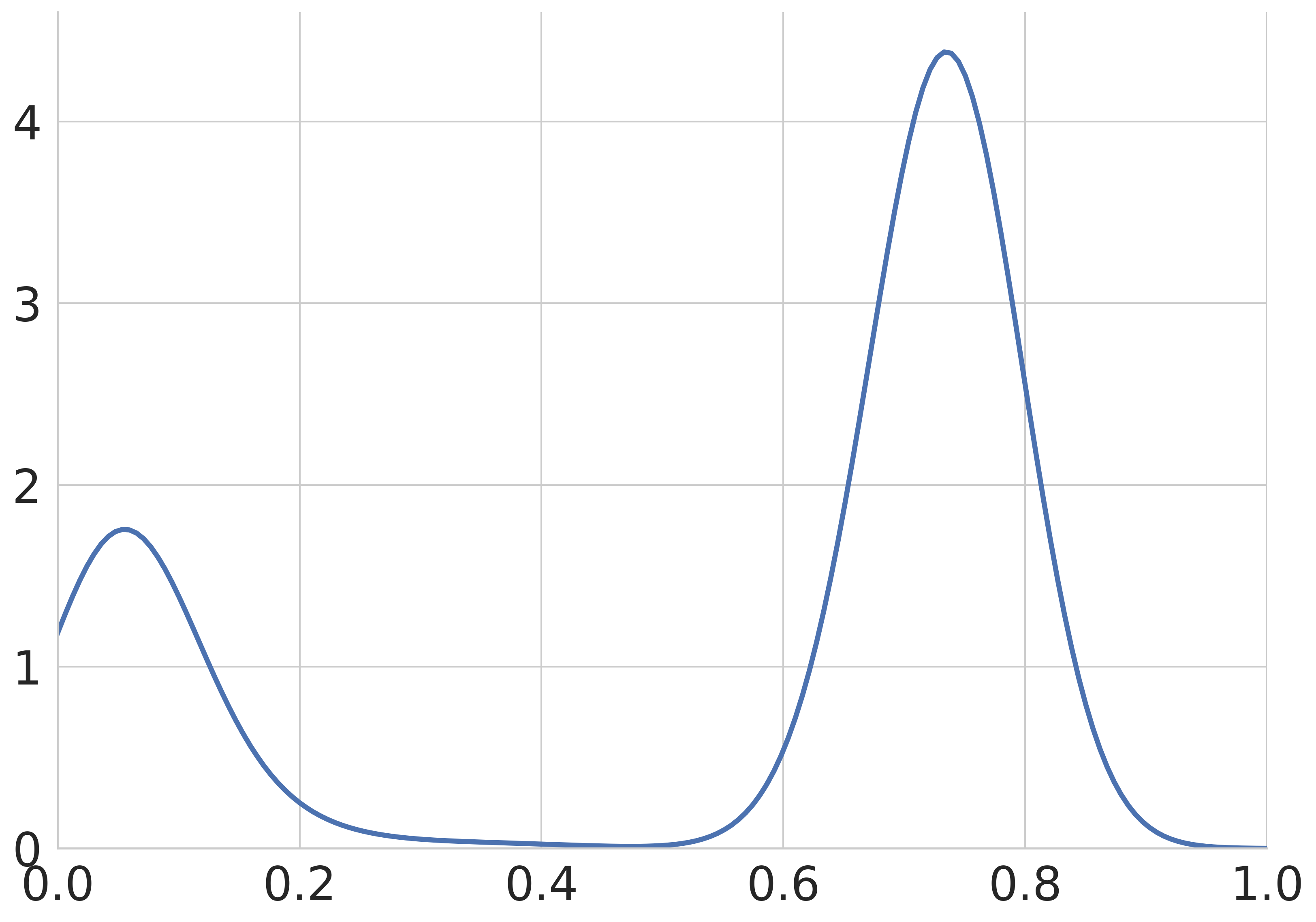
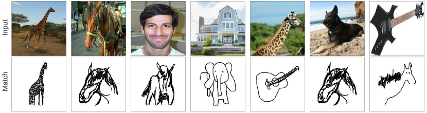
In this section we perform some initial experiments on PACS dataset [45] (using features extracted for a pre-trained CLIP [56] model) to show how the temperature scaling can be used to smooth the propensity score distribution to better control how many sample are discarded during matching. There are 1,670 photo, 2,048 art painting, 2,344 cartoon, and 3,929 sketch in the dataset. Here will evaluate the results of matching across the two domains photo and art painting as well as across photo and sketch. In Fig. 5 and Fig. 6 we compare the shape of the estimated propensity score with its scaled version using a temperature value of 10. As we can see, in the case of a distribution with extremely heavy tails (photo, sketch), the effect of smoothing the distribution is that when a fixed caliper is applied most of the samples are retained. On the other hand, when the initial distribution is smoother, a temperature of 10 is extreme, having the effect of transforming the bimodal distribution to a unimodal one. Additionally, we tabulate in Table 5 the number of matched pairs retrieved when matching across the two domains photo and sketch; here we can see that by increasing the temperature we smooth the estimated propensity score distribution and thereby retain more samples. Similarly, we can retrieve more pairs by reducing the fixed caliper threshold. We also analyse the case of matching across the two domains photo and art painting. Using a fixed caliper defined defined by a threshold and no temperature scaling (i.e. ) the algorithm retrieves 1,142 pairs matching in the direction photo art and 1,501 in the direction art photo.
In Fig. 7 and Fig. 8 we show examples of matching pairs found using our \CNN algorithm. Although the features were not fine-tuned on PACS, we can see a few examples of intraclass matching. For the photo-art painting application we can see preservation in colour and background; while in the photo-sketch case shape and pose.
| Fixed Caliper () | Temperature () | photo sketch | sketch photo |
| 0.1 | 1 | 0 | 0 |
| 0 | 1 | 1540 | 3929 |
| 0.01 | 1 | 6 | 9 |
| 0.01 | 1.3 | 14 | 56 |
| 0.01 | 1.8 | 25 | 574 |
| 0.01 | 2.5 | 41 | 3082 |
| 0.01 | 10 | 1540 | 3929 |
| 0.1 | 10 | 298 | 3929 |
Appendix I Energy and Carbon Footprint Estimates
To highlight the efficiency of Okapi, we provide estimates in 6 of the carbon footprint associated with the running of it and of the ERM and FixMatch baselines on the iWildCam dataset, using the same hyperparameter configuration used to generate the results in the main text. The runs were conducted in a controlled fashion, using the computing infrastructure and device count in all cases.
| Method | kgCOeq |
| ERM | 1.36 |
| FixMatch | 2.12 |
| Okapi (ours) | 1.97 |