MuMIC - Multimodal Embedding for Multi-label Image Classification with Tempered Sigmoid

Abstract

Multi-label image classification is a foundational topic in various domains. Multimodal learning approaches have recently achieved outstanding results in image representation and single-label image classification. For instance, Contrastive Language-Image Pretraining (CLIP) demonstrates impressive image-text representation learning abilities and is robust to natural distribution shifts. This success inspires us to leverage multimodal learning for multi-label classification tasks, and benefit from contrastively learnt pretrained models.

We propose the Multimodal Multi-label Image Classification (MuMIC) framework, which utilizes a hardness-aware tempered sigmoid based Binary Cross Entropy loss function, thus enables the optimization on multi-label objectives and transfer learning on CLIP. MuMIC is capable of providing high classification performance, handling real-world noisy data, supporting zero-shot predictions, and producing domain-specific image embeddings.

In this study, a total of 120 image classes are defined, and more than 140K positive annotations are collected on approximately 60K Booking.com images. The final MuMIC model is deployed on Booking.com Content Intelligence Platform, and it outperforms other state-of-the-art models with $85.6\%$ GAP@10 and $83.8\%$ GAP on all 120 classes, as well as a $90.1\%$ macro mAP score across 32 majority classes. We summarize the modelling choices which are extensively tested through ablation studies. To the best of our knowledge, we are the first to adapt contrastively learnt multimodal pretraining for real-world multi-label image classification problems, and the innovation can be transferred to other domains.

1 Introduction

Multi-label image classification has been widely studied with supervised learning approaches, from various Convolutional Neural Networks (CNNs) based models (O’Shea and Nash 2015) to Vision Transformers (Dosovitskiy et al. 2020). Transfer learning on pretrained models becomes the first choice for many domain-specific applications.

At Booking.com, there are more than 350 million images from multiple sources. Understanding image content is crucial for both travellers and property owners, which makes image classification a core component serving as the backbone of many applications, as described in Section 6.

To drive the various use cases, we need the ability to classify images to a large set of possible labels at a massive scale. The first step is to formulate a label definition list to cover the most important classes. In Section 3, we describe the label definition, label hierarchy, and the annotation procedure. Besides the predefined labels, new travel trends would probably require us to predict on unseen classes. Thus, we need an efficient and scalable solution with zero-shot learning abilities.

We first explore state-of-the-art (SOTA) multi-label classification methods which rank high in open image datasets. They typically handle two main challenges: label imbalance, and extracting features from different regions for multiple objects. To handle the label imbalance, Ridnik et al. (2021a) introduces Asymmetric Loss (ASL) that down-weights and hard-thresholds easy negative samples, while also decouples the penalties on misclassifying the positive and negative samples, which is a novel improvement compared to Focal Loss (Lin et al. 2017). For the second challenge, many methods are proposed to learn semantic label embeddings and attentions to visual features, like cross-modality attention (You et al. 2020), and Query2Label (Liu et al. 2021). However, all the above approaches do not show zero-shot abilities. ML-decoder (Ridnik et al. 2021c) is another SOTA method, which proposes a new classifier head supporting efficient training on large number of classes, and can generalize to unseen classes. However, the zero-shot setting requires specific group-decoding designs, and uses one shared projection matrix in the group fully-connected layer for all classes, which involves additional model training and might cause performance drop. Hence, we do observe the gaps between the current SOTA methods and our requirements.

We further explore image representation learning works and aim to find zero-shot potential and robust pretrained models. It has recently been shown that contrastive representation learning on images is superior to learning from equivalent predictive objectives (Tian, Krishnan, and Isola 2019). One specific approach is using natural language processing (NLP) supervision on images to contrastively enforce better learning of visual concepts (Zhang et al. 2020). NLP supervision enables zero-shot transfer ability to generalize to unseen image-text matching patterns, and can leverage on broad image-text datasets.

CLIP (Radford et al. 2021) is a top performer that uses such NLP supervision, trained on 400 million image-text pairs, and provides robust as well as efficient image representations. CLIP trains multiple image encoding backbones - 5 ResNets (He et al. 2016) and 3 Vision Transformers (ViT) (Dosovitskiy et al. 2020), and shows that ViT provides more computational efficiency which allows production of high performance models. As for image classification, CLIP mainly shows the performance on single-label tasks. To demonstrate transfer learning ability, CLIP focuses on benchmarking zero-shot performance based on image-text embedding similarity, and few-shot linear classifiers. It does not demonstrate fine-tuned results but indicates high potential on it.

Our primary focus is on training visual and text transformers in an image-text pairs pattern with a modified loss function for multi-label classification. The paper’s contributions can be summarized as follow:

• We design a practical MuMIC framework by introducing a hardness-aware loss function - tempered sigmoid based Binary Cross Entropy (BCE) - for multi-label classification, and leveraging on transfer learning from CLIP.

• We share the core findings during the model development, including: theoretically how the sigmoid temperature controls the strengths of penalties on hard samples, as well as how to tune it practically; enrichment on class context (label-text) representation; domain specific image preprocessing etc.

• We study and share efficient and practical dataset annotation strategies, as described in Section 3.

• We compare the final best model’s performance to two baselines: ASL and CLIP. We visualize the improved MuMIC image embedding and compare it with CLIP.

• We provide zero-shot capability for unseen classes, which performs better than CLIP when the unseen class is in the travel domain, and improves product scalability.

• We deploy the final product at Booking.com, and share the main deployment findings.

2 Approach

Given a batch of $N$ images, and $L$ labels, we have $N\times L$ image-label pairs. MuMIC generates $N\times L$ pairs of $(I,T)$, where $I$ is an image embedding, and $T$ is a label embedding (represents the class context). MuMIC is designed to predict which of the labels are relevant and present in the image.

Our general approach is adapting CLIP to support multi-label classification, while learning visual perceptions from natural language supervision of class context. Specifically, we apply ViT (Dosovitskiy et al. 2020) as the computer vision backbone, and Transformer (Vaswani et al. 2017) as the text backbone; with initialized weights from pretrained CLIP, we further fine-tune on the travel domain-specific dataset. This section describes the main proposed method.

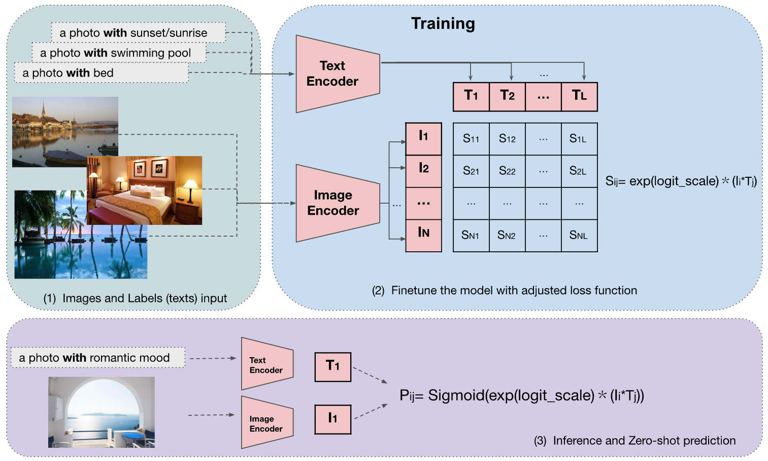
Figure 1: MuMIC architecture. (1) Each label is represented as a label-text like “a photo with {label name}”, or “a photo with {label description}”. The Image Encoder input is a batch of preprocessed images. The Text Encoder input is a list of vectors (each vector is a tokenized label-text). The $S_{ij}$ is MuMIC output logit on image $i$ and label $j$. (2) For inference and zero-shot prediction, MuMIC generates predication scores ($P_{ij}$) for image and label-text by - apply temperature scaling on (image, text) embeddings’ cosine similarity, and then apply sigmoid function on the scaled cosine similarity.

2.1 Main Framework

MuMIC learns a multimodal embedding space by jointly training an image encoder and text encoder to maximize the cosine similarity of the image and label-text embeddings of real labels, as shown in Figure 1. We apply tempered sigmoid based BCE loss on each class and then mean-reduce it (see equation 1), optimizing across all classes.

The Listing 1 describes MuMIC’s core implementation, and demonstrates changes on top of CLIP. Instead of getting image-caption pairs as input, we input a batch of images, together with a list of tokenized texts where each text is derived from either the class name, or the class description.

Listing 1 Numpy style pseudocode mumic_core.py

⬇

1# image_encoder - Vision Transformer

2# text_encoder - Text Transformer

3# I[n, h, w, c] - minibatch of aligned images

4# T[n_c, l] - vector of tokenized label-text (n_c is #classes, l is #tokens)

5# W_i[d_i, d_e] - learned image proj

6# W_t[d_t, d_e] - learned text proj

7# targets[n, n_c] - the ground truth

8# logit_scale - the logit_scale param, = ln(1/temperature)

9

10# extract feature representations of each modality

11I_f = image_encoder(I) #[n, d_i]

12T_f = text_encoder(T) #[n_c, d_t]

13

14# joint multimodal embedding

15I_e = l2_normalize(np.dot(I_f, W_i), axis=1) # [n, d_e]

16T_e = l2_normalize(np.dot(T_f, W_t), axis=1) # [n_c, d_e]

17

18# scaled pairwise cos similarities [n, n_c]

19logits = np.dot(I_e, T_e.T) * np.exp(logit_scale)

20# loss - only need image level loss

21loss = nn.BCEWithLogitsLoss(logits, targets)

2.2 Binary Cross Entropy Loss, based on Tempered Sigmoid

BCE Loss

With each input image $i$, given the ground-truth multi-label vector $y_{i}$, we apply below BCE loss function:

$$L_{BCE}=-\frac{1}{N}\frac{1}{L}\sum_{i=1}^{N}\sum_{j=1}^{L}({p_{j}y_{ij}\cdot\log\sigma(x_{ij})}$$ (1)

$${+(1-y_{ij})\cdot\log(1-\sigma(x_{ij}))}$$

where $\sigma(\cdot)$ is the Tempered Sigmoid function; $x_{ij}$ is the original output logits (before applying temperature scaling), which is the pairwise image-text cosine similarity score on image $i$ and class $j$; and $p_{j}$ is the positive samples weight of class $j$. A higher $p_{j}$ indicates that positive samples are given greater weight, increasing the penalty for identifying false negatives.

As shown in line 21 of Listing 1, we combine the BCE loss with the tempered sigmoid calculation in one single layer. It is more numerically stable by taking advantage of the log-sum-exp trick, which is widely used in machine learning (Nielsen and Sun 2016).

Tempered Sigmoid

As described in (Papernot et al. 2021), the tempered sigmoid function family has 3 hyperparameters - scale, temperature, and offset. Considering we are only using tempered sigmoid for the output layer, we do not use the scale and offset parameters, and the formula we apply is:

$$\begin{split}\sigma(x)&=\frac{1}{1+\exp(-x/\tau)}\\ &=\frac{1}{1+\exp(-x\cdot\exp(logit\_scale))}\end{split}$$ (2)

where $\tau$ is the temperature, $logit\_scale$ is the log-parameterized multiplicative scalar as mentioned in Listing 1 line 8, and $x\cdot\exp(logit\_scale)$ is the output logit.

Why our BCE Loss is hardness-aware

Tempered losses are recently found to provide robustness to noise during training (Amid et al. 2019). Wang and Liu (2020) provides a theoretical proof on why temperature makes softmax-based contrastive loss hardness-aware, and balances the closeness tolerance as well as the ability to learn separable features. Papernot et al. (2021) applies tempered sigmoid activations to replace unbounded activation functions like RELU, and show better performance on noisy data.

In multi-label classification problems, sigmoid-based BCE is widely used. We are inspired by the above mentioned papers, to experiment on adding temperature for sigmoid function at the last layer, and use the temperature to make BCE a hardness-aware loss function. With the BCE loss formula, we can derive the gradient of the loss function to the original logits value $x_{ij}$ (for image $i$ and class $j$):

$$\frac{\partial L_{BCE}(x_{ij},y_{ij})}{\partial x_{ij}}=\frac{1}{\tau}(\sigma(x_{ij})-y_{ij})$$ (3)

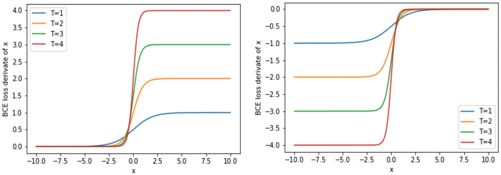
Figure 2: Our BCE loss’s derivative of x. Left side: for negative samples. Right side: for positive samples.

In Figure 2 we visualize the above partial gradient function, where $T$ is the inverse temperature. From both formula and plots, it is clear that temperature plays a significant role in controlling the strength of penalties on hard samples. We observe that with smaller temperature (higher $T$), the derivative of loss has larger magnitude, which is proportional to the gap between the prediction probability ($\sigma(x_{ij})$) and the ground truth ($y_{ij}$). Thus, the loss is more sensitive to hard samples and will enforce stronger improvements on them. In Section 5, we conclude the impact of different temperature levels by showing ablation experiments results, and also compare with normal BCE loss ($\tau$ as 1).

2.3 Image Preprocessing

For image preprocessing, CLIP applies random square crop on resized images for training, and center square crop on resized images for inference. With our use case, it could happen that objects appear at the long edge side. For example, shower and bathtub are sometimes not the central focus of a bathroom image. The square crops could cut them out, while we’d like to recognize them. Our experimental studies show that feeding original images resized to $224\times 224$ with no cropping yields best results as we do not lose important information about a whole scene, and so it is chosen as our final image preprocessing approach. For example, the average precision on TV/Multimedia, and Coffee facilities, are improved by 8.5%, and 7.3% respectively, by removing the cropping step as described above.

3 In-house Dataset Construction

In this section, we describe the creation of the Booking.com multi-label image annotation dataset.

3.1 Class Label Definition

We create a representative label list covering the majority of potential applications. The final list has a total of 120 classes and 8 categories. For each class, we define a label name, a label description, and assign one category for it. One example of a label name is “Historical structure”, which is described as “historical structure, a building or structure with historical value”, and is assigned to the “Outside” category. The 120 classes contain both tangible objects with different sizes (e.g. mirror, kitchen), and intangible items (e.g. winter, sunset). Besides that, there are hierarchical patterns: for example, “Swimming pool” class is a parent of both “Indoor swimming pool” class and “Outdoor swimming pool” class.

3.2 Annotation Collection

Image Candidate Selection

Considering the natural class imbalance, we apply two strategies to generate image samples from the Booking.com database:

1) Enrich image diversity: knowing which property each image belongs to, we apply stratified sampling considering the property features, for example property type (e.g. Villa). 2) Enrich low-resource classes: given the image embedding from the original CLIP, we apply similarity searches with queries on each class, and randomly sample from the top images. For example, query “a photo with dog”, “a photo with cat” for the Pets class. Since Booking.com has a substantial image dataset, we limit the image searching scope with practical rules.

Annotation Question Design

We use AWS SageMaker Ground Truth and Mechanical Turk to collect annotations. This subsection describes how we get full annotation.

AWS provides quality control on the annotator pool, however, the quality could still variate with different tasks. We apply two steps to improve the quality: 1) Assign each annotation task to 5 annotators, and calculate the voting rate per image per label, to infer final ground truth. 2) Smart grouping: given one image, we can either ask 120 binary questions, or group labels into multi-choice questions. We annotate a “golden ground truth” set, design different grouping strategies, and evaluate the annotators’ performance. We find: binary questions get highest recall but lower precision, and cost the most; it’s recommended to put mutually-exclusive labels in one group; never put many difficult labels together; it’s advisable to make each question focusing on one scenario (e.g. Fireplace, Ceiling Fan and Air-conditioner in one group) and have generally 4-6 choices per group.

Consolidation and Dataset Results

As stated above, we collect voting rate results from 5 annotators per image per class. Our evaluation on the golden ground truth set shows: with voting agreement threshold as 0.6, for the majority of classes, both precision and recall are high and near 0.95; for a few difficult classes, the annotation recall is typically higher than precision. Based on the annotation quality evaluation per class, we define customized agreement thresholds for each class. Besides that, we also apply the hierarchical mapping to improve the dataset quality: if one image is labeled as one class, then the class’s parents are also marked as positive. We finally acquire more than 140K positive labels, and 7 million negative labels, on around 60K images.

Even with all above practical improvements, the dataset still contains noise, which is a common challenge for real-world problems. We can tune the temperature of the loss function, and make it more tolerant to noise. The experimentation findings are shared in Section 5.2.

4 Experimental Setup

All of our experiments are performed on a computation instance equipped with 1 NVIDIA Tesla T4 Tensor Core GPU, 4 vCPU, and 16GB RAM. The final best-performing model has the following settings: CLIP ViT-B/32 as the pretrained model; batch size of 64 images with full annotations; weight decay (on all weights that are not gains or biases) with coefficient 0.01, with AdamW optimizer (Loshchilov and Hutter 2017) and learning rate 1e-5; positive class weight as 10 for all classes. Since we apply different image preprocessing from CLIP, use our own label-text input, and aim to get in-house image embeddings, we mainly experiment with unfreezing the image and text encoding backbones.

We split the dataset into training set, validation set, and test set, with a ratio of 80/10/10 respectively. Since we have a class imbalanced multi-label dataset, we apply stratified sampling according to the lowest frequency label per image.

To accelerate training and save memory, we apply the mixed-precision (Micikevicius et al. 2017) strategy as CLIP does. During forward pass and backward propagation, half-precision is applied on the convolutional layers, linear layers, multi-head attention layers, text projection and image projection layers. For the weight update step, the full precision is applied to prevent underflow. The training takes roughly 40 minutes per epoch.

4.1 Evaluation Metrics

Assume the number of labels is $L$, and given $N$ image samples, the ground truth and the predictions can both be represented as a matrix with size $N\times L$. As Sorower (2010) mentioned, the evaluation is to compare these two matrices and determine how close they are. Comparisons can be made in three ways: column-by-column (also called label-based), row-by-row (example-based), or as a whole. We use below metrics as our main evaluation criterion:

• Average Precision per class (label-based):

  $$AP_{j}=\sum_{i=1}^{N}p_{j}(i)\Delta r_{j}(i)$$ (4)

  where $p_{j}$ is the precision of class $j$, and $r_{j}$ is the recall of class $j$. It is equivalent to the area under the precision-recall curve per class.

• macro Mean Average Precision (aggregate on label-based):

  $$macro\>mAP=\frac{1}{L}\sum_{j=1}^{L}AP_{j}$$ (5)

  which is the unweighted average of AP across all classes.

• weighted Mean Average Precision (aggregate on label-based):

  $$weighted\>mAP=\frac{1}{\sum_{j=1}^{L}{NP_{j}}}\sum_{j=1}^{L}AP_{j}\cdot NP_{j}$$ (6)

  where $NP_{j}$ is the number of positive samples of class $j$.

• Global Average Precision (global-based):

  $$GAP=\sum_{i=1}^{N\cdot L}p(i)\Delta r(i)$$ (7)

  GAP (also called micro mAP (Yang 1999)) is implemented as: collect predictions from all classes, and calculate the area under the global precision-recall curve.

• GAP@K: for each sample, take the top K predictions according to probability ranking, and calculate GAP on top of the collected predictions from all samples.

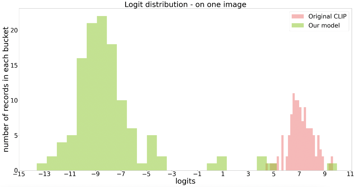
Figure 3: Output logits distribution - on one image, across 120 label-texts (“a photo with {label name}”).

4.2 Baselines

We implement two baselines as follows:

• ASL (Ridnik et al. 2021a): ASL authors provide a collection of high performance models trained on various multi-label datasets (Ridnik et al. 2021b). We fine-tune the MS-COCO (Lin et al. 2014) based TResNet (Ridnik et al. 2020) large model, on our dataset, and apply hyperparameter tunes to get top-performing ASL model.

• Original CLIP (Radford et al. 2021): Given one image, CLIP was trained with the main objective as distinguishing one text from all others. Figure 3 shows the output logits distribution from CLIP and MuMIC - on one image example. We observe that CLIP majority outputs are centered around value 7 for all classes, while MuMIC can distinguish between positive classes and negative ones. That is because CLIP was optimized for single-label with softmax-based loss, not for multi-label. To generate multi-label predictions with CLIP, one approach is taking top $K$ output logits per image. However, it’s not feasible to define a proper unified $K$. Instead, we apply the following approach: for each class, input a pair of text - “a photo”, “a photo of {label name}”; apply softmax on the two output logits, and use the second probability as the label prediction.

5 Results and Development Findings

In this section, we explain the final model performance and other experimental findings.

5.1 Final Model Performance

method	GAP	GAP@10	macro mAP	weighted mAP
CLIP	32.7	44.5	56.7	56.1
ASL	67.7	77.3	60.8	68.9
MuMIC	83.8	85.6	74.7	79.5

Table 1: Performance comparison of MuMIC against 2 baselines, on the test set, 120 classes. All metrics are in %.

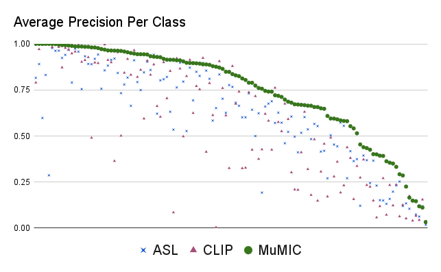
Figure 4: AP on each class, on the test set. The x axis represents the 120 classes (decreasing order on MuMIC AP).

Table 1 and Figure 4 show how the final MuMIC model outperforms the two baselines. From Figure 4, we observe that MuMIC outperforms the other 2 baselines across large majority of the labels. Furthermore, we see a few classes for which none of the compared methods achieve satisfactory results. Our investigation shows two main reasons: these classes are more noisy since they are challenging and not easily distinguished even by a human (e.g. Toaster, Patio); they are still too low frequent. Table 2 shows AP scores on some classes as examples. For general class like Bed or Food, all methods show acceptable performance. For more travel domain related classes, model training is necessary. For example, Animal in travel does not include pets, and there are various types of Lobby, where we observe the original CLIP performance is not enough.

method	Golf	Bed	Win- ter	Food	Lob- by	Animal (not pets)
CLIP	94.8	95.8	91.2	90.0	50.1	49.0
ASL	79.0	97.4	93.3	91.3	73.3	89.0
MuMIC	98.9	98.6	98.4	96.4	96.2	98.1

Table 2: Average Precision (AP) on some classes - MuMIC against 2 baselines on the test set. All metrics are in %.

Regarding the training time efficiency, the ASL training time per epoch is similar to MuMIC (40 minutes as Section 4 shows), but ASL takes around 18 epochs to saturate, while MuMIC only needs around 3 epochs. That indicates MuMIC training efficiency is boosted by the large-scale pretrained CLIP, and the hardness-aware loss function. Regarding the inference time, CLIP’s text encoding time is twice that of MuMIC, since CLIP requires a pair of text inputs per class.

5.2 Temperature Factor Selection

As described in Section 2, the temperature $\tau$ is an important factor. CLIP initializes the contrastive loss temperature as 0.07 (empirical value from Wang and Liu (2020)), and clips the value at around 0.01 to prevent training instability. We also decide to initialize temperature, make it a parameter for the model to learn with capping value, instead of freezing it as a hyperparameter. Since we have a real-world noisy dataset, and are fine-tuning on top of pretrained models, we find it is necessary to search the best initialization temperature for the tempered sigmoid.

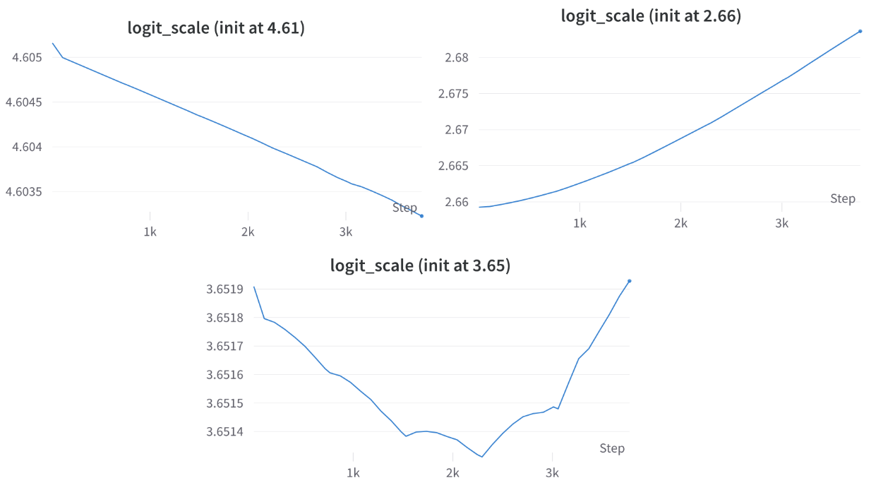
Figure 5: Param $logit\_scale$ learning curve examples

logit_scale init value	0.703	0.913	2.005	2.578	2.659	2.927	3.352	3.652	4.189	4.605	5.244	5.751
macro mAP	17.5	22.8	65.9	72.2	72.6	73.7	73.9	74.1	73.9	73.1	73.1	72.6
GAP@10	56.1	62.1	78.5	83.9	83.9	84.7	85.0	85.4	85.0	84.4	84.4	84.1

Table 3: Validation set performance - with different temperature initialization values

We perform Bayesian optimization (Mockus, Tiesis, and Zilinskas 1978) search to find a proper setting. Table 3 shows the validation set performance with various initialization values. Our best $logit\_scale$ initialization value is $3.652$, which outperforms the cases when initializing $\tau$ either as 0.07 ($logit\_scale$ $2.659$), or as the pretrained CLIP $\tau$ value ($logit\_scale$ $4.605$). Figure 5 shows how the network learns to optimize $logit\_scale$ during training steps.

From both Table 3 and Figure 5, we observe it is important to start $\tau$ from a proper value. If the temperature is too small, the strict penalties on hard samples might make the model too sensitive to noise like wrong annotations. If the temperature is too big, then the penalties on hard samples could be not enough and limit the model’s learning ability. In addition, we run an experiment with normal sigmoid-based BCE loss (freeze $\tau$ at value 1), the validation set can reach a maximum macro mAP score of 43.3% and GAP@10 score of 38.2%, which are far lower than MuMIC performance.

5.3 Enrich Class Context with Class Description

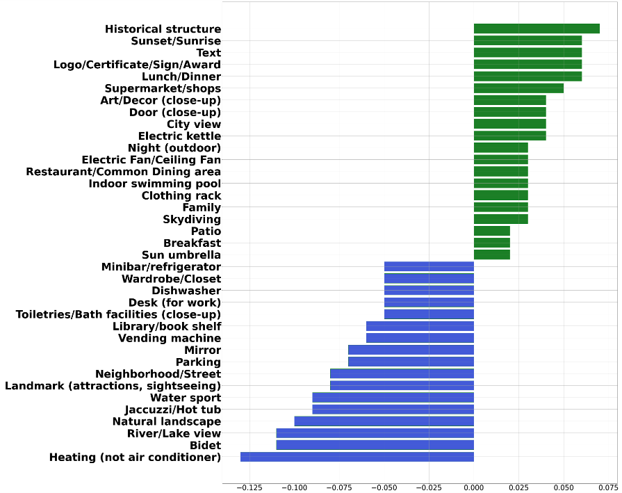
Figure 6: Validation set AP gap examples. The x axis is the AP gap: using class description minus using class name.

As described in Section 2, we experiment with either using “a photo with {label name}”, or “a photo with {label description}” as the input text representing a label. This leads to label description being used across a subset of labels that benefit from it, as the upper side examples shown in Figure 6. More convenient labels like Parking and Mirror prefer concise class names rather than descriptions, in comparison to labels like Art/decor, Historical structure where descriptions improve the label-text embedding and the performance.

5.4 Image Embedding

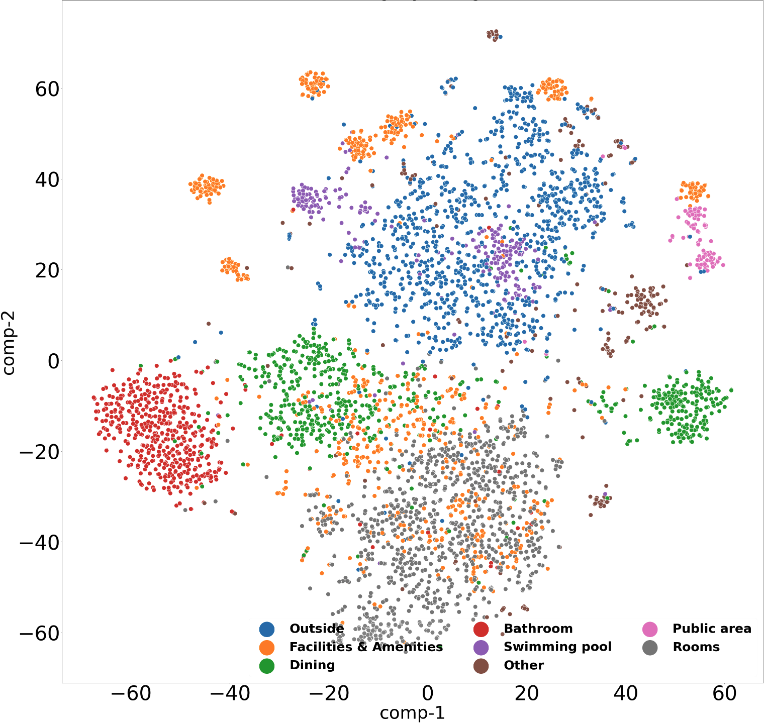
Figure 7: t-SNE on category - original CLIP

Figure 8: t-SNE on category - MuMIC

MuMIC generates travel domain image embeddings which can be applied to downstream machine learning applications (e.g. gallery embedding to find similar hotels). Figure 7 and 8 display the t-SNE (Van der Maaten and Hinton 2008) visualizations of image embeddings on the test set, colored at the category level. When an image has multiple labels, we color the point with the lowest frequent class’s category, to acquire more samples for low resource categories. From the two figures, MuMIC has better ability to enforce differentiation among different categories. We also analyze t-SNE distributions on the class level, and reach similar conclusions.

5.5 Zero-shot Learning

With multimodal learning, we expect semantic information to propagate from seen classes to the unseen ones. As the predefined 120 classes covered main travel topics, MuMIC can generalize well to unseen travel domain labels.

Figure 9 and 10 show zero-shot prediction examples from MuMIC and CLIP. For MuMIC, we apply sigmoids on the 5 output logits to get prediction scores. For CLIP, we apply two approaches: multi-label as Section 4.2 described; and single-label via softmax on the 5 output logits. MuMIC gets high scores on correct labels (internal museum, mountain climbing etc.), and low scores on wrong labels (shopping, door etc.), indicating good generalization. Comparing with MuMIC, CLIP multi-label approach gets quite high scores on wrong labels. CLIP single-label approach has the top K selection problem as Section 4.2 explained.

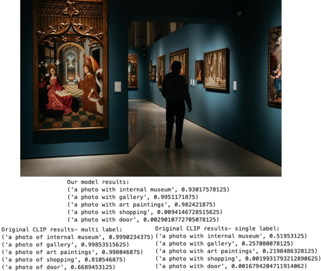
Figure 9: Zero-shot Prediction examples - Museums

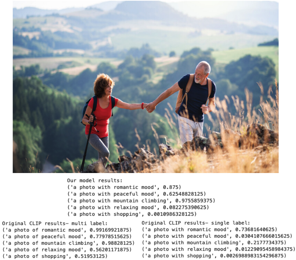
Figure 10: Zero-shot Prediction examples - Trip types

6 Application Examples

The final MuMIC model supports multiple downstream use cases. For each application, online A/B test (Fabijan et al. 2018) is required to be conducted on real traffic of Booking.com and typically lasts for several weeks. Below are application examples that can benefit from MuMIC:

Main gallery subset selection By default, the gallery subset/preview on the property page contains the first images uploaded. MuMIC can be applied to select more representative subset to cover different aspects - building, room, bathroom, dining area, etc. Figure 11 shows one example: the left side is before applying the model, where we see duplicate bedroom images, and an image with long text; the right side is the new design, shows better gallery quality. This A/B test results in +0.5% more users progressing to the next step of the booking funnel, indicates better user engagement.

Content selection a) Native ads - the image classification results are applied in a combination with an image quality model in order to select the best images for native ads. The A/B test results in +5% more clicks on ads. b) Destination recommendation - some destinations have no image on their recommendation cards. With image classification results on outdoor classes (natural landscape, street, sightseeing, etc.), we are able to re-purpose gallery photos and use them for supplementing missing destination images. The A/B test results in +4.3% more clicks on the cards.

Content validation and enrichment - identifying mismatches between the facilities reported by the property owners and the ones existing in property’s photos, and enabling owners to take actions. This is currently in production on Booking.com partner website, with property owners adopting 96% of the recommended gaps. When customers filter for a certain facility, for example swimming pool, they are able to see and book more properties with swimming pools.

7 Deployment and Maintenance

The final MuMIC model is served with Amazon SageMaker, and deployed on Booking.com Content Intelligence Platform (CIP) - a stream processing platform based on Apache Flink, that consumes real-time events (e.g. requests on image prediction) from Kafka topics, and generates model-based results. The final product provides both real-time predictions services, and backfilling services.

The backfilling jobs run MuMIC on Booking.com image datasets, store the predictions, image embeddings and metadata to databases. Thus, consumers can retrieve results from a central place, instead of sending and managing requests on the overlapping images per use case. To save storage space, we decide to only save the label predictions above certain thresholds. We perform thresholds selection per class on the validation and test set, by analyzing the percentage of data we can drop and the maximum recall still remain. We finally drop around 87% of data while keep the recall close to 1.

The model is served on GPU instances instead of CPU, since our analysis shows that to predict on same amount of images, the cost on using GPU is around 3 times less than CPU. It’s also worth mentioning the model inference endpoints support batch predictions, which is shown to be roughly 5 times faster than predicting images one by one. The above optimizations match our expectations, since the MuMIC architecture is highly parallelizable because of the transformers backbones.

To achieve system robustness and scalability, we apply auto-scaling, which leads to a better handling on peak times, and a lower cost on off-peak times. In addition, model serving metrics (e.g. throughput, inference time) are monitored using in-house dashboards and AWS CloudWatch.

8 Conclusion

Multi-label image classification is a crucial task for many domains. In this paper, we present MuMIC, a multimodal approach for multi-label image classification based on contrastively learnt CLIP model. Our main novelty lies in the creation of an in-house dataset for the travel industry, and application of supervised multimodal learning with tempered-sigmoid based BCE loss. We perform ablation studies and show the impact of different choices, including temperature tuning, and class context enrichment with class descriptions.

Our development, performed on a real-world Booking.com dataset, demonstrates that MuMIC is a practical framework that outperforms SOTA approaches in both classification performance and training efficiency. With MuMIC framework, the model also learns high quality in-domain image embeddings, and acquires zero-shot learning abilities on unseen classes without additional training.

For future work, we suggest improving the low performance labels, by refining class definitions and representations, reducing annotation noise, and assigning higher loss weights. Few-shot learning for new classes on top of MuMIC embeddings could also be a promising direction.

Figure 11: Gallery subset display

References

- Amid et al. (2019) Amid, E.; Warmuth, M. K.; Anil, R.; and Koren, T. 2019. Robust Bi-Tempered Logistic Loss Based on Bregman Divergences. CoRR, abs/1906.03361.
- Dosovitskiy et al. (2020) Dosovitskiy, A.; Beyer, L.; Kolesnikov, A.; Weissenborn, D.; Zhai, X.; Unterthiner, T.; Dehghani, M.; Minderer, M.; Heigold, G.; Gelly, S.; et al. 2020. An image is worth 16x16 words: Transformers for image recognition at scale. arXiv preprint arXiv:2010.11929.
- Fabijan et al. (2018) Fabijan, A.; Dmitriev, P. A.; McFarland, C.; Vermeer, L.; Olsson, H. H.; and Bosch, J. 2018. Experimentation growth: Evolving trustworthy A/B testing capabilities in online software companies. Journal of Software: Evolution and Process, 30.
- He et al. (2016) He, K.; Zhang, X.; Ren, S.; and Sun, J. 2016. Deep Residual Learning for Image Recognition. In 2016 IEEE Conference on Computer Vision and Pattern Recognition (CVPR), 770–778.
- Lin et al. (2017) Lin, T.; Goyal, P.; Girshick, R. B.; He, K.; and Dollár, P. 2017. Focal Loss for Dense Object Detection. CoRR, abs/1708.02002.
- Lin et al. (2014) Lin, T.; Maire, M.; Belongie, S. J.; Bourdev, L. D.; Girshick, R. B.; Hays, J.; Perona, P.; Ramanan, D.; Dollár, P.; and Zitnick, C. L. 2014. Microsoft COCO: Common Objects in Context. CoRR, abs/1405.0312.
- Liu et al. (2021) Liu, S.; Zhang, L.; Yang, X.; Su, H.; and Zhu, J. 2021. Query2Label: A Simple Transformer Way to Multi-Label Classification. CoRR, abs/2107.10834.
- Loshchilov and Hutter (2017) Loshchilov, I.; and Hutter, F. 2017. Fixing Weight Decay Regularization in Adam. CoRR, abs/1711.05101.
- Micikevicius et al. (2017) Micikevicius, P.; Narang, S.; Alben, J.; Diamos, G.; Elsen, E.; Garcia, D.; Ginsburg, B.; Houston, M.; Kuchaiev, O.; Venkatesh, G.; and Wu, H. 2017. Mixed Precision Training. Cite arxiv:1710.03740Comment: Published as a conference paper at ICLR 2018.
- Mockus, Tiesis, and Zilinskas (1978) Mockus, J.; Tiesis, V.; and Zilinskas, A. 1978. The Application of Bayesian Methods for Seeking the Extremum. Towards Global Optimization, 2(117-129): 2.
- Nielsen and Sun (2016) Nielsen, F.; and Sun, K. 2016. Guaranteed bounds on information-theoretic measures of univariate mixtures using piecewise log-sum-exp inequalities. Entropy, 18(12): 442.
- O’Shea and Nash (2015) O’Shea, K.; and Nash, R. 2015. An introduction to convolutional neural networks. arXiv preprint arXiv:1511.08458.
- Papernot et al. (2021) Papernot, N.; Thakurta, A.; Song, S.; Chien, S.; and Erlingsson, . 2021. Tempered Sigmoid Activations for Deep Learning with Differential Privacy. Proceedings of the AAAI Conference on Artificial Intelligence, 35(10): 9312–9321.
- Radford et al. (2021) Radford, A.; Kim, J. W.; Hallacy, C.; Ramesh, A.; Goh, G.; Agarwal, S.; Sastry, G.; Askell, A.; Mishkin, P.; Clark, J.; et al. 2021. Learning transferable visual models from natural language supervision. In International Conference on Machine Learning, 8748–8763. PMLR.
- Ridnik et al. (2021a) Ridnik, T.; Ben-Baruch, E.; Zamir, N.; Noy, A.; Friedman, I.; Protter, M.; and Zelnik-Manor, L. 2021a. Asymmetric loss for multi-label classification. In Proceedings of the IEEE/CVF International Conference on Computer Vision, 82–91.
- Ridnik et al. (2021b) Ridnik, T.; Ben-Baruch, E.; Zamir, N.; Noy, A.; Friedman, I.; Protter, M.; and Zelnik-Manor, L. 2021b. Asymmetric loss for multi-label classification. https://github.com/Alibaba-MIIL/ASL.
- Ridnik et al. (2020) Ridnik, T.; Lawen, H.; Noy, A.; and Friedman, I. 2020. TResNet: High Performance GPU-Dedicated Architecture. CoRR, abs/2003.13630.
- Ridnik et al. (2021c) Ridnik, T.; Sharir, G.; Ben-Cohen, A.; Ben-Baruch, E.; and Noy, A. 2021c. Ml-decoder: Scalable and versatile classification head. arXiv preprint arXiv:2111.12933.
- Sorower (2010) Sorower, M. S. 2010. A literature survey on algorithms for multi-label learning. Oregon State University, Corvallis, 18: 1–25.
- Tian, Krishnan, and Isola (2019) Tian, Y.; Krishnan, D.; and Isola, P. 2019. Contrastive Multiview Coding. CoRR, abs/1906.05849.
- Van der Maaten and Hinton (2008) Van der Maaten, L.; and Hinton, G. 2008. Visualizing data using t-SNE. Journal of machine learning research, 9(11).
- Vaswani et al. (2017) Vaswani, A.; Shazeer, N.; Parmar, N.; Uszkoreit, J.; Jones, L.; Gomez, A. N.; Kaiser, Ł.; and Polosukhin, I. 2017. Attention is all you need. Advances in neural information processing systems, 30.
- Wang and Liu (2020) Wang, F.; and Liu, H. 2020. Understanding the Behaviour of Contrastive Loss. CoRR, abs/2012.09740.
- Yang (1999) Yang, Y. 1999. An evaluation of statistical approaches to text categorization. Information retrieval, 1(1): 69–90.
- You et al. (2020) You, R.; Guo, Z.; Cui, L.; Long, X.; Bao, S. Y.-Z.; and Wen, S. 2020. Cross-Modality Attention with Semantic Graph Embedding for Multi-Label Classification. ArXiv, abs/1912.07872.
- Zhang et al. (2020) Zhang, Y.; Jiang, H.; Miura, Y.; Manning, C. D.; and Langlotz, C. P. 2020. Contrastive Learning of Medical Visual Representations from Paired Images and Text. CoRR, abs/2010.00747.