An Interpretable Machine Learning System to Identify EEG Patterns on the Ictal-Interictal-Injury Continuum

Abstract

In intensive care units (ICUs), critically ill patients are monitored with electroencephalograms (EEGs) to prevent serious brain injury. The number of patients who can be monitored is constrained by the availability of trained physicians to read EEGs, and EEG interpretation can be subjective and prone to inter-observer variability. Automated deep learning systems for EEG could reduce human bias and accelerate the diagnostic process. However, black box deep learning models are untrustworthy, difficult to troubleshoot, and lack accountability in real-world applications, leading to a lack of trust and adoption by clinicians. To address these challenges, we propose a novel interpretable deep learning model that not only predicts the presence of harmful brainwave patterns but also provides high-quality case-based explanations of its decisions. Our model performs better than the corresponding black box model, despite being constrained to be interpretable. The learned 2D embedded space provides the first global overview of the structure of ictal-interictal-injury continuum brainwave patterns. The ability to understand how our model arrived at its decisions will not only help clinicians to diagnose and treat harmful brain activities more accurately but also increase their trust and adoption of machine learning models in clinical practice; this could be an integral component of the ICU neurologists’ standard workflow.

Introduction

Chiappa et al. [22] hypothesize that brainwave activity lies along a spectrum, the “ictal-interictal-injury continuum” (IIIC): patterns at one end of this continuum are hypothesized to cause brain injury and are difficult to distinguish from seizures on the EEG; patterns at the other bear little resemblance to seizures and are thought to cause little to no harm. Seizures and status epilepticus are found in 20% of patients with severe medical and neurologic illness who undergo brain monitoring with electroencephalography (EEG) because of altered mental status [27, 17], and every hour of seizures detected on EEG further increases the risk of permanent disability or death [7, 21]. More ambiguous patterns of brain activity, consisting of periodic discharges or rhythmic activity, are even more common, occurring in nearly 40% of patients undergoing EEG monitoring [18]. Two recent studies found evidence that, like seizures, this type of prolonged activity also increases the risk of disability and death [30, 20]. Although the IIIC hypothesis has gained wide acceptance [5, 13], categorizing IIIC patterns has been difficult because, until recently, the only method for quantifying IIIC patterns has been manual review of the EEG, which suffers from subjectivity due to the ambiguous nature of the IIIC patterns and scales poorly to large cohorts [23, 22].

Progress in machine learning (“AI”) and the availability of large EEG datasets has recently made it possible to develop an automated algorithm (SPaRCNet) [15] to detect and classify IIIC patterns with a level of accuracy comparable to physician experts [11]. However, like most AI approaches, SPaRCNet is uninterpretable, meaning that it cannot explain how it reaches its conclusions. As we train deep learning models for clinical tasks, the lack of interpretability or “black-box” nature of these models has been identified as a barrier to deployment in clinical settings [24]. Black-box (a.k.a. uninterpretable) models are prone to silent failures during normal operations by not generalizing to real-world conditions [3] or by relying on features irrelevant to the task [31], misleading clinicians and putting patients at risk. Ideally, we would instead prefer an interpretable model, where the clinician could review the reasoning of the model for logical consistency and plausibility given current medical knowledge. The replacement of a black-box model with an interpretable model could improve the utility, safety, and trustworthiness of the system – and, ideally, can be done with no loss in accuracy.

To address the challenges of the black-box models and introduce interpretability into the workflow of EEG monitoring, we present ProtoPMed-EEG, a novel interpretable deep learning algorithm to classify IIIC activities and visualize their relationships with each other. ProtoPMed-EEG is more accurate than its uninterpretable counterpart (SPaRCNet) and provides an explanation of every prediction through comparisons to learned prototypical patterns. We create a graphical user interface (GUI) leveraging the learned interpretable model and a global-structure preserving dimension reduction technique, enabling inspection of relationships and distances between EEG patterns and “mapping” of the IIIC in a 2D space. We explicitly demonstrate the underlying continuum among pathological patterns of brain activity, which sheds new light on how we understand and analyze EEG data. The ability to understand how our model arrived at its decisions will not only help clinicians to diagnose and treat harmful brain activities more accurately but also increase their trust and adoption of machine learning models in clinical practice; this could be an integral component of the ICU neurologists’ standard workflow.

The main contributions of our paper are as follows:

• We introduce ProtoPMed-EEG, an interpretable deep-learning algorithm to classify seizures and rhythmic and periodic EEG patterns. Explanations are of the form “this EEG looks like that EEG,” the TEEGLLTEEG explanation method. Our proposed interpretable algorithm outperforms its black-box counterpart in both classification performance and interpretability metrics.

• We develop a GUI tool for user inspection of the learned latent space, providing explanations for the model predictions.

• We map the IIIC into a 2D space, revealing that EEG patterns within the IIIC, despite being given distinct class names, do not exist in isolated islands. Rather, each class is connected to every other class via a sequence of transitional intermediate patterns, which we demonstrate in a series of videos.

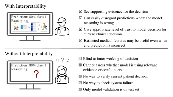
Figure 1: The benefits of an interpretable model in the clinic.

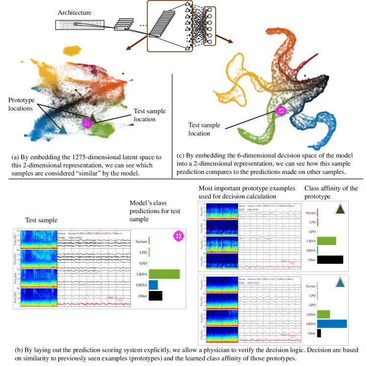
Figure 2: Three different ways an end user can see how the model reasons about the test sample.

Methods

EEG Data and Expert Labels

ProtoPMed-EEG was trained and tested on a large-scale EEG study [16] consisting of 50,697 events from 2,711 patients hospitalized between July 2006 and March 2020 who underwent continuous EEG as part of clinical care at Massachusetts General Hospital. EEG electrodes were placed according to the International 10-20 system. The large group was intended to ensure broad coverage of all variations of IIIC events encountered in practice. 124 EEG raters from 18 centers labeled varying numbers of 10-second EEG segments in 2 stages. Raters were given a choice of six options: seizure (SZ), lateralized periodic discharges (LPD), generalized periodic discharges (GPD), lateralized rhythmic delta activity (LRDA), generalized rhythmic delta activity (GRDA), and “Other” if none of those patterns was present. The data labeling procedure is described further in Appendix A. Mean rater-to-rater inter-rater reliability (IRR) was moderate (percent agreement 52%, $\kappa$ 42%), and mean rater-to-majority IRR was substantial (percent agreement 65%, $\kappa$ 61%). As expert annotators do not always agree, we evaluate our model against the “majority vote,” such that the class selected by the most raters is the ground truth for each sample. This allows us to demonstrate that the model performs as well as an expert human annotator.

Model Interpretability

In this paper, we define interpretable models as models that “explain their predictions in a way that humans can understand” [24]. In Figure 2, we display three different ways an end user can see how the model reasons about the test sample. Figure 2c shows the model’s final classification of the test sample relative to previous cases. Figure 2a shows how the model perceives the test sample relative to previous cases. Figure 2b shows how the model uses case-based reasoning to make its prediction. Case-based reasoning is defined as using previous examples to reason about a new case. During training, the model learns a set of previous cases called prototypical samples. Each prototypical sample is a 50-second EEG sample from the training set that is particularly useful for classifying new cases. For each prediction, the model generates similarity scores between the new case and the set of prototypical samples. Each explanation is of the form “this sample is class X because it is similar to these prototypes of class X, and not similar to prototypes of other classes.” We call this method the TEEGLLTEEG explanation method because it makes explanations of the form “this EEG looks like that EEG.” Every prediction made by our model follows the same logic as the explanation provided by the model. This means that the model explanations have perfect fidelity with the underlying decision-making process, by design.

Model Training and Development

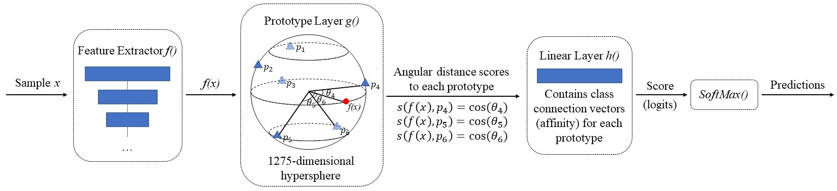
Figure 3: Model architecture. Input sample $x$ is passed through a feature extractor $f()$, followed by a prototype layer $g()$. The prototype layer calculates the angular distances between the sample feature and the prototypes. The angular distances are multiplied with class affinity to generate the logits (class scores). The softmax calculation converts the logits into prediction probabilities.

Our dataset consists of 50-second EEG samples $x_{i}$ with class labels $y_{i}$ indicating the EEG pattern. The patients were split into approximately equally sized training and test sets. So that any prototypical sample will have a more detailed label, samples with higher counts of expert votes ($\geq 20$) were selected from the training set to form the prototype set of cases that are candidates to become prototypical samples.

ProtoPMed-EEG is an adaptation of ProtoPNet, a convolutional neural network model with a prototype interpretability layer, built on recent work by Li et al. [19], Chen et al. [4], and Barnett et al. [2], incorporating angular similarity as in Donnelly et al. [10]. The network architecture for ProtoPMed-EEG is shown in Figure 3. Our model consists of feature extraction layers $f()$, which are initialized by weights from Jing et al. [15]; prototype layer $g()$, which computes the similarity (angular distance) between each learned prototype and feature extractor output $f(\mathbf{x})$ for each sample $\mathbf{x}$; and a final linear layer $h()$, which maps the similarity to each prototype into class scores for each EEG pattern using class-connection vectors. The set of $m$ prototypes is $P=\{p_{j}\}_{j=0}^{m}$, where each prototype is a vector of length 1275 that exists in the same 1275-dimensional latent space as outputs $f(\mathbf{x})$. Each learned prototype corresponds to an actual EEG sample from the prototype set, where $f(\mathbf{x}_{i^{\prime}})$ is the prototype corresponding to the prototypical sample $\mathbf{x}_{i^{\prime}}$. Network layer $h()$ is initialized such that the first 30 prototypes are single-class prototypes (that is, being similar to the prototype increases the class score for one of the EEG patterns) and the next 15 prototypes are dual-class prototypes (that is, being similar to the prototype increases the class score for two of the EEG patterns). The model is trained with an objective function containing loss terms to encourage accuracy, a clustering structure in the latent space and separation between prototypes. Training is completed in 4 hours using two Nvidia V100 GPUs.

Refer to Appendix B for further information on model architecture and training.

Graphical User Interface

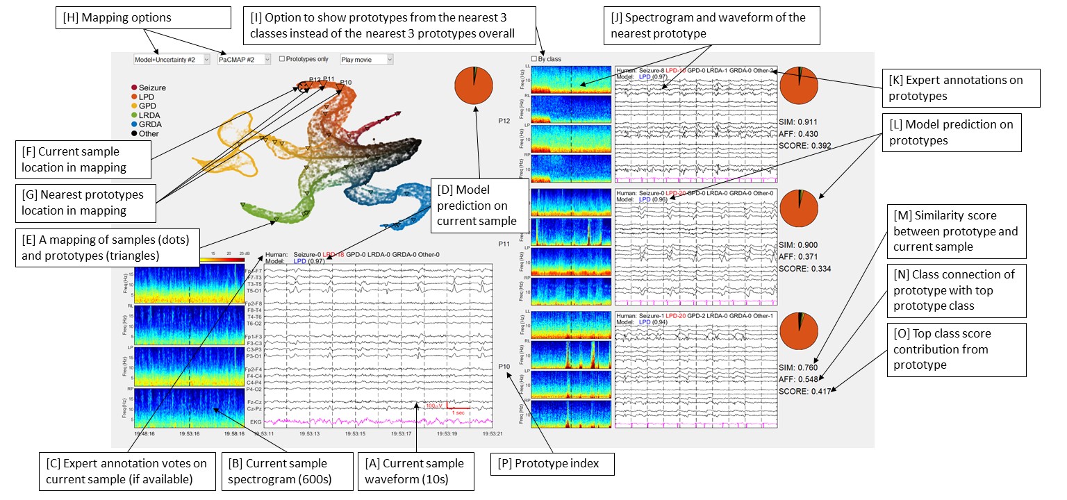
Figure 4: The graphical user interface (GUI) of the interpretable system. On the left top panel is the 2D embedding map, with each dot representing one EEG sample. Dots can be displayed with shading according to 9 different available schemes (human majority, model prediction, model uncertainty, Seizure burden etc.). A user can click on the map to select any sample of interest; the 3 nearest prototypes are displayed on the right, ranked according to similarity score (SIM). For each sample/prototype, 10 seconds of the EEG and a 10-minute spectrogram (centered on the 10-second EEG segment) are displayed with human votes and model predictions shown on top of the EEG; a pie chart is provided to visualize the class distribution according to the model or human votes, depending on the selected color scheme. For each prototype, under its pie chart, we also list the values of three terms: similarity score (SIM), class connection (AFF), and class contribution score (SCORE).

We also present a specialized graphical user interface (GUI) that allows users to explore the interpretable model and its predictions on the test set. A screenshot is shown in Figure 4. On the bottom left of the GUI, we present the waveform [A], spectrogram [B], and the expert-annotator votes [C] of the currently selected sample. Below the expert-annotator votes, we display the model prediction [D] on the currently selected sample. On the upper left of the GUI, we present the 2D representation of the latent space that was generated using PaCMAP [E]. We can see the location of the current sample [F], as well as the location of the nearest prototypes [G] in the 2D representation. The color schema and mapping methods can be changed using drop-down menus [H]. Which prototypes are displayed can be changed using a selection box [I], where one option shows the nearest prototypes regardless of class and the other shows the nearest prototype from each of the three highest-score classes. Along the right-hand side, we display the waveform, spectrogram [J], expert-annotator votes [K] and model prediction [L] for the prototypical samples from the three displayed prototypes (in this case, the three nearest prototypes). For each of the displayed prototypes, we show the similarity score between the prototypical sample and the currently selected sample [M], the class-connection between the prototype and the predicted class (affinity) [N] and the class score added by that prototype to the predicted class [O].

Evaluation of Model Performance

We evaluate our model’s performance using area under receiver operating characteristic curve (AUROC) scores, area under precision-recall curve (AUPRC) scores and neighborhood analysis measures. For comparing AUROC scores between the black box model and ours, we use the Delong test [8] for statistical significance. For AUPRC comparisons, we test for statistical significance using the bootstrapping method with 1000 bootstrap samples. For more detail on these statistical significance tests, refer to Appendix D. We further evaluated model performance using neighborhood analysis. Details are provided in the Results section.

Role of the Funding Source

None.

Results

Model Performance

The classification performance of our interpretable model ProtoPMed-EEG statistically significantly exceeds that of its uninterpretable counterpart SPaRCNet in distinguishing Seizures, LPDs, GPDs, LRDAs, and GRDAs, as measured both by AUROC and AUPRC scores (p<0.001). Results for ROC and PR curve analysis are shown in Figures 6(a), 6(b), and 5. These findings hold when bootstrapping by patient or by sample. The main contribution of this method is the increased interpretability; increased performance is a secondary finding.

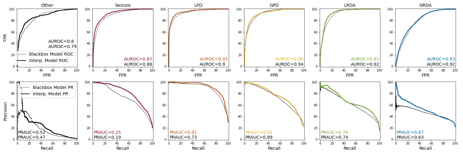
Figure 5: The receiver operating characteristic curves and precision-recall curves for ProtoPMed-EEG (solid lines) compared to its uninterpretable counterpart SPaRCNet (dashed lines).

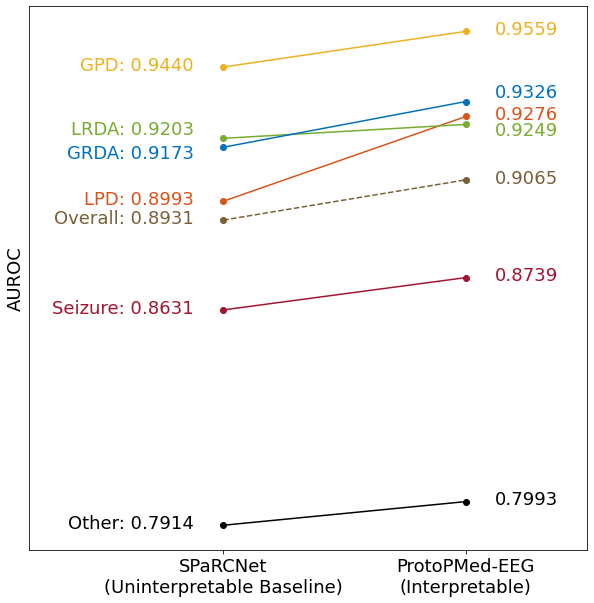
(a) AUROC Comparisons

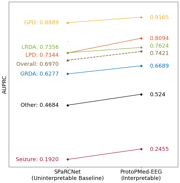
(b) AUPRC Comparisons

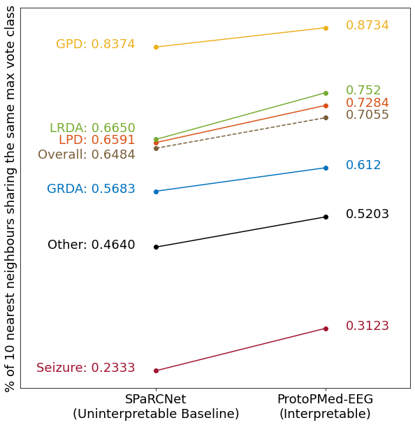
(c) Neighborhood analysis by max

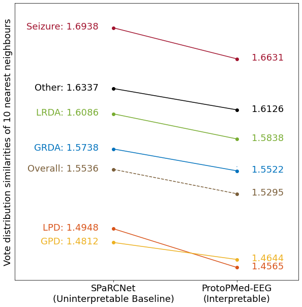
(d) Neighborhood analysis by annotator vote distribution (lower score demonstrates a more consistent neighborhood)

Figure 6: The four slope charts comparing (a) AUROC scores, (b) AUPRC scores, (c) neighborhood analysis by max vote and (d) neighborhood analysis by annotator vote distributions between the uninterpretable SPaRCNet[15] and our interpretable ProtoPMed-EEG. The uncertainty bounds for each point are smaller than the point itself. Higher values are desired for all metrics except ’neighborhood analysis by annotator vote distribution’ in (d).

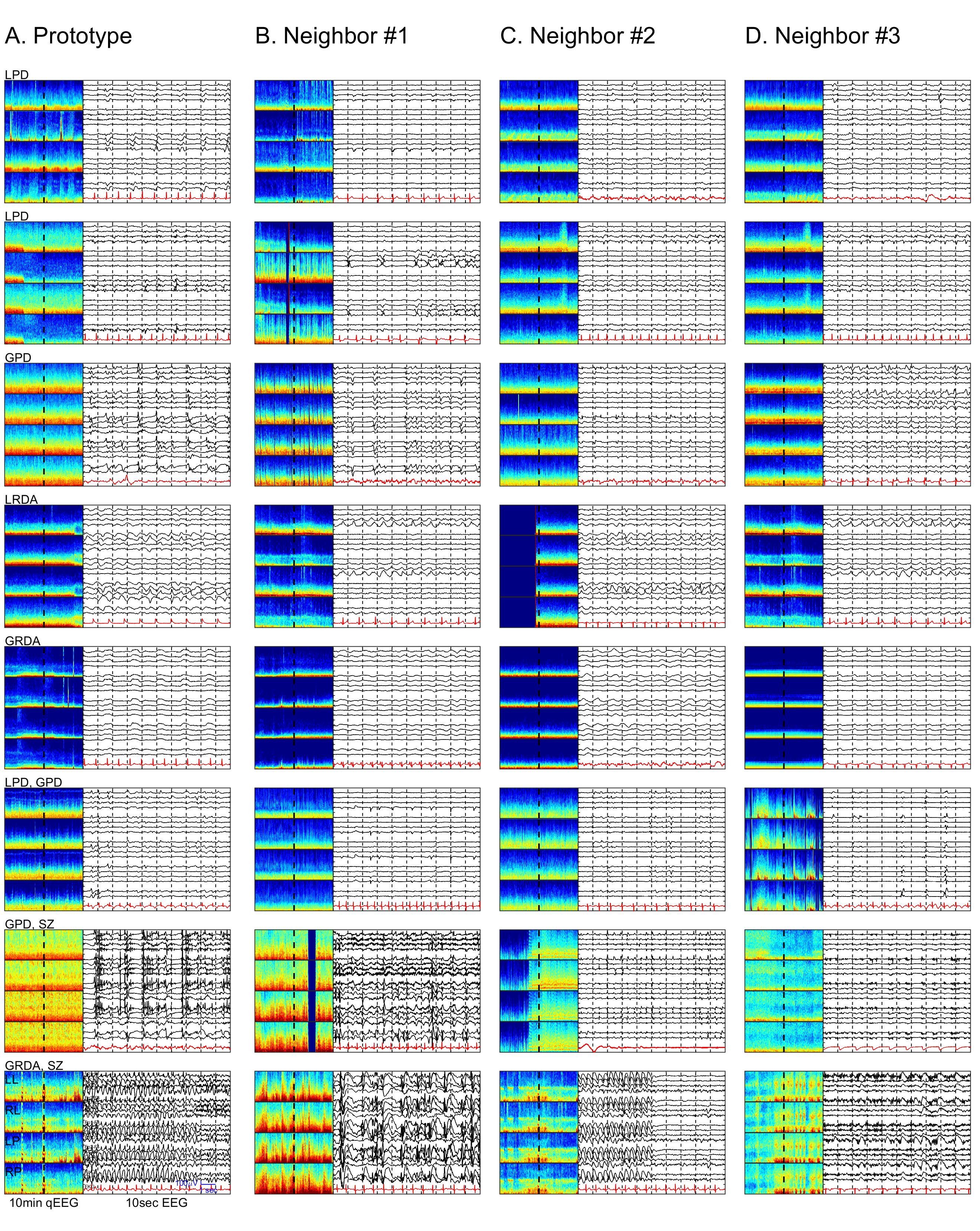
Figure 7: The nearest neighbors for a prototype of the ProtoPMed-EEG model. We show top 3 nearest test samples corresponding to the prototype in 8 cases. The full set of prototypes and their neighbors can be found in Appendix E.

Model Interpretability Quantitative Performance Evaluation

As one way to evaluate the interpretability of ProtoPMed-EEG, we perform a neighborhood analysis. Specifically, we analyzed the neighborhood of each prototype to examine the structure of the learned latent space. In a well-trained system, the neighborhood of a $c$-class prototype will primarily contain samples from class $c$. For each sample in the test set, we calculate the percentage of the 10 nearest test set neighbors where the class with the most votes is the same as for the sample (“by max”). We also consider the neighborhood analyses “by vote,” where for each sample, we calculate the mean cross-entropy of the vote distribution of the sample with the vote distribution of each of the 10 nearest neighbors. Here, we consider cross entropy as a discrete distribution across classes and check whether the cross entropy of the test point matches the distribution of classes from the nearest neighbors. The interpretable model does statistically significantly better than its uninterpretable counterpart across all metrics and classes with $p<0.05$ for each comparison (see Figure 6(c) and 6(d)).

Model Interpretability Qualitative Performance Evaluation

For the system to be understandable, we require that samples in the neighborhood around a prototype are also qualitatively similar to the prototype according to domain experts. In Figure 7, for each of the eight prototypes from our model, we explore the three nearest neighbors from the test set to the prototype. In each case, the neighboring samples are similar to the prototype not only in class but also in amplitude, peak-to-peak distance and other domain-relevant qualities. This demonstrates to domain experts our model’s concept of “similarity.” Qualitative neighborhood analyses for all prototypes showing the six nearest neighbors from each of the training and test sets can be found at https://warpwire.duke.edu/w/fzoHAA/.

Mapping the Ictal-Interictal-Injury Continuum

In Figures 2c and 4, the coloring and distance between samples (points) are based on the model class scores for each sample. This results in a structure with outer points (arms) corresponding to single classes and reveals dense, thread-like paths mapping a gradual change between IIIC classes. This lends credence to the concept of a “continuum” between ictal and interictal EEG patterns; a set of well-separated classes would instead be represented by disconnected islands. This morphology is consistent across models initiated with different random seeds. We further sampled along those paths between each pair of IIIC patterns, and produced videos demonstrating the smooth continuum from one pattern to the other. Videos are provided at https://warpwire.duke.edu/w/8zoHAA/.

Discussion

In this study, we developed an interpretable deep learning model to classify seizures and rhythmic and periodic patterns of brain activity that occur commonly in patients with severe neurologic and medical illness. We introduced a specially-designed graphical user interface to explore the interpretable model. Each explanation follows the TEEGLLTEEG explanation method (“this EEG looks like that EEG.”) This is the first adaption of interpretable neural networks to cEEG and the first quantitative exploration of the ictal-interictal-injury continuum. The model is trained on a large and diverse set of EEG signals annotated by multiple independent experts, and evaluated against the current state-of-the-art black box model. Our work yielded advancements in both the model performance and model interpretability. Compared to the black box baseline model, our model achieves significant improvements in pattern classification performance as measured by AUROC and AUPRC. We also achieve better neighborhood analysis scores, indicating that the interpretable model learned a more class-consistent neighborhood in the latent space.

While machine learning, and specifically deep learning, has been used for EEG classification tasks including seizure detection [15, 28, 6], our interpretable model goes beyond traditional tasks, providing clinicians with the means to validate diagnoses and providing researchers verifiable evidence for smooth continuity of the IIIC, confirming the existence of an underlying continuum. Although there are past works on leveraging prototypes to provide explanations for model predictions [32, 14, 12], the prototypes were limited to single classes which is insufficient for mapping IIIC patterns, as evidenced by the common occurrence in our dataset of patterns on which expert opinions are divided as to the correct classification. Our introduction of dual-class prototypes enables our model to place prototypes between two classes in the latent space, providing insights into EEG patterns in the transitional states.

Due to the existence of samples between classes in the EEG pattern classifications, particularly the transitional states, human annotations often yield disagreements. Our interpretable model can provide additional support for clinicians in day-to-day ICU patient monitoring. The model provides prediction along with its neighborhood and matched prototype information to users, allowing users to evaluate the reliability of predictions, thereby acting as an “assistant” in the process. Since our GUI provides expert annotation records alongside model predictions, this tool may also be helpful in training clinicians; our case-based-reasoning design would provide not only explanations for model predictions but also insights for existing expert annotations.

Limitations

In our dataset, the number of seizure class samples was substantially smaller compared to other classes. We alleviated the class imbalance issue during the training process, however, a more balanced dataset would be helpful for achieving better performance. More seizure data samples could also help the model learn a better set of seizure prototypes with more robust representations. In future studies, we could also leverage the additional 10-minute spectrogram information as it is also a component in the human decision process.

The interpretability is limited to the final steps of the model, so a clinician must still infer how the relevant qualities (i.e., peak-to-peak distance, amplitude, burst suppression ratio) are weighed in the model’s assessment of similarity. In cases where this is not clear, the qualitative neighborhood analyses are available for examination. An area of future work would be to account for known qualities of interest explicitly. Despite this limitation, the interpretability provided by this model greatly surpasses all similarly-performing models.

Conclusion

In this study, we developed an interpretable deep learning algorithm that accurately classifies six clinically relevant EEG patterns, and offers faithful explanations for its classifications leveraging prototype learning. Our results challenge the common belief of an accuracy-interpretability trade-off. The comprehensive explanations and the graphical user interface allow for follow-up testing working toward clinical applications, including diagnostic assistance and education.

Conflict of Interest Disclosures

Dr. Westover is a co-founder of Beacon Biosignals, which played no role in this work.

Author Contribution Statement

Idea conception and development: Alina Jade Barnett, Zhicheng Guo, Jin Jing, Brandon Westover, Cynthia Rudin. Interpretable model code: Zhicheng Guo, Alina Jade Barnett. GUI code: Jin Jing. Data preparation: Jin Jing, Zhicheng Guo, Alina Jade Barnett, Wendong Ge. Writing: Alina Jade Barnett, Zhicheng Guo, Jin Jing, Brandon Westover, Cynthia Rudin.

Appendix A Dataset and Labeling

The process for data annotation and train-test split are the same as in Jing et al. [16] and [15].

124 independent raters from 18 institutions were asked to label the central 10 seconds of cEEG clips as one of: seizure (SZ), lateralized periodic discharges (LPD), generalized periodic discharges (GPD), lateralized rhythmic delta activity (LRDA), generalized rhythmic delta activity (GRDA), and “Other” if none of those patterns was present. Each of the 50,697 cEEG event samples has between 10 and 20 ratings, referred to in this paper as “votes.” Only the samples with over 20 votes were allowed to become prototypes (i.e., added to the prototype set).

Appendix B Model Details

Our model, ProtoPMed-EEG, is developed from IAIA-BL (Interpretable AI Algorithms for Breast Lesions) from Barnett et al. [2], which is based on ProtoPNet from Chen et al. [4]. We also incorporate angular similarity as in Deformable ProtoPNet [10] and TesNet [29].

B.1 Model Architecture

Let $D=\{\mathbf{x}_{i},y_{i}\}_{i=0}^{n}$ be our dataset of $n$ 50-second EEG samples $\mathbf{x}$ with class labels $y$ indicating the EEG pattern of Seizure, LPD, GPD, LRDA, GRDA, or Other. Refer to Figure 3 for a diagram of the model architecture. Our model consists of feature extraction layers $f_{\omega_{f}}()$, prototype layer $g_{\omega_{g}}()$ and final linear layer $h_{\omega_{h}}()$. For the $i^{\text{th}}$ EEG sample, corresponding model prediction $\hat{y}_{i}$ is calculated as

$$\hat{y}_{i}=h_{\omega_{h}}(g_{\omega_{g}}(f_{\omega_{f}}(\mathbf{x}_{i}))).$$ (1)

The feature extraction layers $f_{\omega_{f}}()$ consist of all but the final layer of the neural network architecture from Jing et al. [15], which was trained on the same dataset. The model architecture from Jing et al. [15] was designed to handle 10-second samples, where (when removing the final layer) the output for a single 10-second EEG sample is a vector of length 255. Our model uses 50-second samples by concatenating the five 10-second outputs into a single 1275-length vector which we will denote as $f_{\omega_{f}}(\mathbf{x})$.

The input to prototype layer $g_{\omega_{g}}()$ is the output from $f_{\omega_{f}}(\mathbf{x})$. The set of $m$ prototypes is $P=\{p_{j}\}_{j=0}^{m}$. Each prototype is a vector of length 1275 that exists in the same 1275-dimensional latent space as outputs $f_{\omega_{f}}(\mathbf{x})$. For each prototype, the similarity score $s$ between test sample $\mathbf{x}$ and prototype $p_{j}$ is

$$s(f_{\omega_{f}}(\mathbf{x}),p_{j})=\left(\frac{af_{\omega_{f}}(\mathbf{x})}{\|f_{\omega_{f}}(\mathbf{x})\|}\right)\cdot\left(\frac{p_{j}}{\|p_{j}\|}\right),$$ (2)

where $a=64$ as in Deng et al. [9]. This similarity score is 0 for orthogonal vectors and 64 for identical vectors.

The prototypes are each given a class identity by final linear layer $h_{\omega_{h}}()$. $h_{\omega_{h}}()$ has size $m\times C$, where $m$ is the number of prototypes and $C$ is the number of classes. We can think of this as a $C$-length vector for each prototype, which determines how similarity to the prototype affects class score. For example, a single-class class-two prototype has a corresponding $C$-length vector in $h_{\omega_{h}}()$ that is initialized as $(-1,-1,1,-1,-1,-1)$. This means that if a sample is similar to this prototype, the score for class two will increase and the score for all other other classes will decrease. (Note that the class indices range from 0 to the number of classes, which is why class 2 is represented by the third index of the vector.) We call this the class connection vector for the prototype. We also introduce dual-class prototypes in this paper. For example, a prototype of both class zero and class five would have class connection vector initialized as $(1,-1,-1,-1,-1,1)$. Though prototypes shared between classes were used in previous work by Rymarczyk et al. [25], their method differs in that it merges similar prototypes whereas our method learns prototypes that are explicitly in-between classes and do not fit into either class individually.

The number of prototypes is selected as a hyperparameter before training, though it is possible to prune prototypes posthoc. If there are too few prototypes, the similarity between a test sample and the displayed prototype will not be clear to the end user. We need enough prototypes to cover the space so that the similarity between any test sample and the nearest prototype is clear. If there are too many prototypes, the model overfits and the latent space has less structure, impairing interpretability (however, we can detect overfitting using a validation set, as usual). We may also end up with duplicate prototypes when there are too many prototypes. For this domain, we decided on 45 prototypes, five single-class prototypes for each class (30 total) and one dual-class prototype for each edge between two classes (15 total, 6 choose 2).

Architecture note: While ProtoPNet [4] and IAIA-BL [2] both have several “add-on” layers between the pre-trained part of $f_{\omega_{f}}()$ and prototype layers $g_{\omega_{g}}()$, this is unnecessary when using a cosine similarity as in Deformable ProtoPNet [10] and our method.

B.2 Model Training

The feature extraction layers $f_{\omega_{f}}()$ are initialized with pretrained weights from the uninterpretable model of Jing et al. [15].

Our model is trained in four stages: (1) warm up, (2) joint training, (3) projection of the prototypes and (4) last layer optimization. Training starts with the warm up stage for 10 epochs. After warm up, the training cycles from joint training for 10 epochs, to the projection step, to last layer optimization for 10 epochs, before returning to joint training for the next cycle. We continue for 80 total epochs, as training typically converges between 30 and 40 epochs.

(1) Warm up. During the warm up stage, only the prototype layer weights in $g_{\omega_{g}}()$ change. We use a learning rate of 0.002. The objective function for the warm up stage is:

$$\min_{\omega_{g}}\left(\mathrm{CrsEnt}+\lambda_{c}~{}\ell_{\mathrm{clst}}+\lambda_{s}~{}\ell_{\mathrm{sep}}+\lambda_{o}~{}\ell_{\mathrm{ortho}}\right),$$ (3)

where $\mathrm{CrsEnt}$ is the cross entropy, $\ell_{\mathrm{clst}}$ and $\ell_{\mathrm{sep}}$ encourage clustering around meaningful prototypes in the latent space and $\ell_{\mathrm{ortho}}$ encourages orthogonality between prototypes. The weights on each loss term are as follows: $\lambda_{c}=-0.8$, $\lambda_{s}=-0.08$, and $\lambda_{o}=100$. Adapted from Chen et al. [4] and Barnett et al. [2] to use cosine similarity instead of L2 similarity,

$$\ell_{\mathrm{clst}}=\frac{1}{n}\sum_{i=1}^{n}\min_{j:\text{class}(\mathbf{p}_{j})=y_{i}}s(f_{\omega_{f}}(\mathbf{x}_{i}),p_{j}),\hskip 14.22636pt\ell_{\mathrm{sep}}=-\frac{1}{n}\sum_{i=1}^{n}\min_{j:\text{class}(\mathbf{p}_{j})\neq y_{i}}s(f_{\omega_{f}}(\mathbf{x}_{i}),p_{j}).$$ (4)

$\ell_{\mathrm{clst}}$ encourages each training sample to be close to a prototype of its own class, and $\ell_{\mathrm{sep}}$ encourages each training sample to be far from prototypes not of its own class. $\ell_{\mathrm{ortho}}$ is defined as

$$\ell_{\mathrm{ortho}}= \frac{1}{a^{2}}\left(\sum_{j=0}^{m}\sum_{j^{\prime}=0}^{m}(s(p_{j},p_{j^{\prime}}))^{2}-\sum_{j=0}^{m}(s(p_{j},p_{j}))^{2}\right)\text{, or equivalently}$$ (5)

$$\ell_{\mathrm{ortho}}= \|\mathbf{P}\mathbf{P}^{T}-I\|_{F}^{2},$$ (6)

where $\mathbf{P}$ is the $m$ by $1275$ matrix of normalized prototype vectors and $\|\|_{F}^{2}$ is the squared Frobenius norm.

(2) Joint training. During joint training, weights from $f_{\omega_{f}}()$, $g_{\omega_{g}}()$ and $h_{\omega_{h}}()$ are all trained simultaneously. We use a learning rate of 0.0002 for training the weights in $f_{\omega_{f}}()$, 0.003 for the weights in $g_{\omega_{g}}()$ and 0.001 for the weights in $h_{\omega_{h}}()$. The objective function is:

$$\min_{\omega_{f},\omega_{g},\omega_{h}}\left(\mathrm{CrsEnt}+\lambda_{c}~{}\ell_{\mathrm{clst}}+\lambda_{s}~{}\ell_{\mathrm{sep}}+\lambda_{o}~{}\ell_{\mathrm{ortho}}+\lambda_{l}~{}\ell_{\mathrm{lll1}}\right),$$ (7)

where $\mathrm{CrsEnt}$, $\ell_{\mathrm{clst}}$, $\ell_{\mathrm{sep}}$, $\ell_{\mathrm{ortho}}$, $\lambda_{c}$, $\lambda_{s}$, and $\lambda_{o}$ are as above, while $\ell_{\mathrm{lll1}}$ is the L1 loss on the weights in the last layer and $\lambda_{l}=0.0001$.

(3) Projection step. During the projection step, we project the prototype vectors on the nearest (most similar) EEG samples from the projection set. The projection set $D^{\prime}$ is the subset of the training set $D$ that has at least 20 expert annotations of the class. This allows us to visualize a prototype as, after projection, the prototype exactly equals the latent space representation of the projection set example. This projection step is

$$p_{j}^{\text{updated}}=f_{\omega_{f}}\left(\underset{\mathbf{x}\in D^{\prime}}{\text{argmax}}\ s\left(f_{\omega_{f}}(\mathbf{x}),p_{j}\right)\right).$$ (8)

(4) Last layer optimization. During last layer optimization, weights from $f_{\omega_{f}}()$ and $g_{\omega_{g}}()$ are frozen and only weights from $h_{\omega_{h}}()$ may change. The learning rate is 0.001 and the objective function is:

$$\min_{\omega_{h}}\left(\mathrm{CrsEnt}+\lambda_{l}~{}\ell_{\mathrm{lll1}}\right),$$ (9)

where $\mathrm{CrsEnt}$, $\ell_{\mathrm{lll1}}$, $\lambda_{l}$ are as above.

Note: We considered using the margin loss from Donnelly et al. [10], which encourages wide separation in the latent space between classes. We noted much worse results when margin loss was included. We speculate that this is because the classes are not clearly separated in this domain, but instead exist on a continuum. With margin loss included, the network is penalized for placing an EEG sample between two classes, yet we know that there exist dual-class samples (i.e., SZ-GPD). This could account for the drop in accuracy when margin loss is introduced.

Appendix C Model Performance Comparison

Table 1: AUROC, AUPRC and neighborhood analysis of the interpretable model compared to its uninterpretable counterpart, SPaRCNet [15]. Each prediction problem is one-vs-all. The column name “All” refers to a mean for all classes weighted by the number of samples in each class. For “Neighborhood Analysis by Votes,” a lower score is better; for all other metrics, a higher score is better. 95% confidence intervals are shown in square brackets. We use the bootstrapping method described in Appendix D.1 for AUPRC and AUROC. We use $\sigma_{u}=\frac{\sigma}{\sqrt{N}}$ for the neighborhood analyses. The test set size $N$ is $35740$ cEEG samples. Our results show statistically significant improvements over SPaRCNet for all comparisons, see Appendix Table 3 for AUROC and AUPRC significance test results and Appendix Table 4 for neighborhood analysis significance test results.

		Other	Seizure	LPD	GPD	LRDA	GRDA	All
AUROC	Interp.	0.80 [0.80, 0.80]	0.87 [0.87, 0.87]	0.93 [0.93, 0.93]	0.96 [0.96, 0.96]	0.92 [0.92, 0.93]	0.93 [0.93, 0.93]	0.91 [0.91, 0.91]
	Uninterp.	0.79 [0.79, 0.79]	0.86 [0.86, 0.86]	0.90 [0.90, 0.90]	0.94 [0.94, 0.94]	0.92 [0.92, 0.92]	0.92 [0.92, 0.92]	0.89 [0.89, 0.89]
AUPRC	Interp.	0.52 [0.52, 0.52]	0.25 [0.24, 0.25]	0.81 [0.81, 0.81]	0.92 [0.92, 0.92]	0.76 [0.76, 0.76]	0.67 [0.67, 0.67]	0.74 [0.74, 0.74]
	Uninterp.	0.47 [0.47, 0.47]	0.19 [0.19, 0.19]	0.73 [0.73, 0.73]	0.89 [0.89, 0.89]	0.74 [0.74, 0.74]	0.63 [0.63, 0.63]	0.70 [0.70, 0.70]
Neighborhood	Interp.	0.52 [0.51, 0.53]	0.31 [0.29, 0.34]	0.73 [0.72, 0.74]	0.87 [0.87, 0.88]	0.75 [0.75, 0.76]	0.61 [0.60, 0.62]	0.71 [0.70, 0.71]
Analysis by Max	Uninterp.	0.47 [0 47, 0.48]	0.23 [0.21, 0.25]	0.65 [0.65, 0.66]	0.84 [0.83, 0.84]	0.67 [0.66, 0.68]	0.56 [0.55, 0.57]	0.65 [0.65, 0.65]
Neighborhood	Interp.	1.61 [1.61, 1.61]	1.66 [1.65, 1.68]	1.46 [1.45, 1.46]	1.46 [1.46, 1.47]	1.58 [1.58, 1.59]	1.55 [1.55, 1.56]	1.53 [1.53, 1.53]
Analysis by Votes	Uninterp.	1.63 [1.63, 1.63]	1.69 [1.68, 1.71]	1.50 [1.49, 1.50]	1.48 [1.48, 1.48]	1.61 [1.60, 1.61]	1.55 [1.55, 1.56]	1.55 [1.55, 1.56]

Appendix D Statistical Significance and Uncertainty Calculations

D.1 Uncertainty Calculation for AUPRC and AUROC using bootstrapping

We take $N=1000$ bootstrap samples of size $|D^{t}|$ with replacement from the test set, where $|D^{t}|$ is the size of the test set. We calculate the AUPRC and AUROC for each bootstrap sample, presenting the median AUPRC or AUROC in Table 1. The 95% CI is calculated by $\mu\pm(1.96)\frac{\sigma}{\sqrt{N}}$, where $\mu$ is the mean AUPRC or AUROC of the 1000 bootstrap samples, $\sigma$ is the standard deviation of the AUPRCs or AUROCs of the 1000 bootstrap samples, and $N$ is equal to the number of bootstrap samples. (Note that one bootstrap sample is made up of $|D^{t}|$ EEG samples.)

D.2 Bootstrap by Patient

We conducted an experiment with an additional bootstrap method where each bootstrap sample consists of the EEG samples from 761 randomly selected patients with replacement from the test set (the test set has 761 patients). Refer to Table 2 for values. Whether bootstrapping by patient, as shown here, or by sample, as shown in the main text, our interpretable method is statistically significantly better than its uninterpretable counterpart.

Table 2: AUROC and AUPRC of the interpretable model compared to its uninterpretable counterpart from Jing et al. [15]. Here we present the results of bootstrapping by patient.

		Other	Seizure	LPD	GPD	LRDA	GRDA	All
AUROC	Interp.	0.80 [0.80, 0.80]	0.87 [0.87, 0.87]	0.93 [0.93, 0.93]	0.95 [0.95, 0.95]	0.93 [0.92, 0.92]	0.93 [0.93, 0.93]	0.91 [0.9, 0.91]
	Uninterp. [15]	0.79 [0.79, 0.79]	0.86 [0.86, 0.86]	0.90 [0.90, 0.90]	0.94 [0.94, 0.94]	0.92 [0.92, 0.92]	0.92 [0.92, 0.92]	0.89 [0.89, 0.89]
AUPRC	Interp.	0.53 [0.52, 0.53]	0.25 [0.25, 0.26]	0.81 [0.81, 0.81]	0.91 [0.90, 0.91]	0.76 [0.75, 0.76]	0.67 [0.67, 0.67]	0.74 [0.74, 0.74]
	Uninterp. [15]	0.47 [0.47, 0.47]	0.19 [0.19, 0.19]	0.73 [0.73, 0.73]	0.89 [0.89, 0.89]	0.74 [0.74, 0.74]	0.63 [0.63, 0.63]	0.70 [0.70, 0.70]

To further test the significance in difference between our interpretable model and the uninterpretable model’s bootstrapped results, we also calculated the percentage of bootstrap samples where interpretable model performs better than the uninterpretable model of Jing et al. [15], shown in Table 3.

Table 3: The percentage of bootstrap samples where interpretable model performs better than the uninterpretable model of Jing et al. [15].

		Other	Seizure	LPD	GPD	LRDA	GRDA	All
AUROC	Sample Bootstrap	98.90	80.60	100.00	100.00	97.90	100.00	100.00
	Patient Bootstrap	62.4	70.40	96.40	77.40	60.00	88.10	77.00
AUPRC	Sample Bootstrap	100.00	98.00	100.00	100.00	100.00	100.00	100.00
	Patient Bootstrap	98.30	86.70	97.20	68.50	64.00	82.00	93.60

D.3 p-values for Neighborhood Analyses

Additional exploration of the statistical significance of our neighborhood analysis results can be found in Table 4. The interpretable model is always significantly better than the uninterpretable model with p-values much lower than 0.001.

Table 4: Here we present the significance (p-values) of the neighborhood analysis results of our interpretable model vs. the uninterpretable model of Jing et al. [15]. The interpretable model was always significantly better.

	Other	Seizure	LPD	GPD	LRDA	GRDA	All
Neighborhood Analysis by Max	3.13e-45	2.26e-12	6.68e-128	1.23e-68	3.64e-134	4.13e-32	0.00
Neighborhood analysis by Vote	3.75e-124	3.47e-09	1.10e0159	2.78e-84	6.41e-132	4.29e-71	0.00

D.4 Reproducibility of the Annoy package for neighborhood analysis calculation

Due to the large amount of data in our study, traditional nearest-neighbor calculations are intractable and we must use approximation code. The state-of-the-art Annoy package [26] is used to find approximate nearest neighbors for our neighborhood analysis metrics. We used the high-computation cost, highest-accuracy setting on this package to extract the nearest neighbors for each sample for neighborhood analysis. In its current implementation, the Annoy approximation algorithm is not fully reproducible, which is a finding brought up by multiple other users. To account for this issue, we ran the algorithm multiple times and compared results, finding that neighborhood analysis results varied by less than 0.01%.

Appendix E Qualitative Neighborhood Analyses

https://warpwire.duke.edu/w/fzoHAA/

Appendix F Videos link

https://warpwire.duke.edu/w/8zoHAA/

References

- [1]
- Barnett et al. [2021] Alina Jade Barnett, Fides Regina Schwartz, Chaofan Tao, Chaofan Chen, Yinhao Ren, Joseph Y Lo, and Cynthia Rudin. 2021. A case-based interpretable deep learning model for classification of mass lesions in digital mammography. Nature Machine Intelligence 3, 12 (2021), 1061–1070.
- Beede et al. [2020] Emma Beede, Elizabeth Baylor, Fred Hersch, Anna Iurchenko, Lauren Wilcox, Paisan Ruamviboonsuk, and Laura M. Vardoulakis. 2020. A Human-Centered Evaluation of a Deep Learning System Deployed in Clinics for the Detection of Diabetic Retinopathy. In Proceedings of the 2020 CHI Conference on Human Factors in Computing Systems (Honolulu, HI, USA) (CHI ’20). Association for Computing Machinery, New York, NY, USA, 1–12. https://doi.org/10.1145/3313831.3376718
- Chen et al. [2019] Chaofan Chen, Oscar Li, Daniel Tao, Alina Barnett, Cynthia Rudin, and Jonathan K Su. 2019. This Looks Like That: Deep Learning for Interpretable Image Recognition. In Advances in Neural Information Processing Systems 32 (NeurIPS). 8930–8941.
- Chong and Hirsch [2005] Derek J Chong and Lawrence J Hirsch. 2005. Which EEG patterns warrant treatment in the critically ill? Reviewing the evidence for treatment of periodic epileptiform discharges and related patterns. Journal of Clinical Neurophysiology 22, 2 (2005), 79–91.
- Craik et al. [2019] Alexander Craik, Yongtian He, and Jose L Contreras-Vidal. 2019. Deep learning for electroencephalogram (EEG) classification tasks: a review. Journal of neural engineering 16, 3 (2019), 031001.
- De Marchis et al. [2016] Gian Marco De Marchis, Deborah Pugin, Emma Meyers, Angela Velasquez, Sureerat Suwatcharangkoon, Soojin Park, M Cristina Falo, Sachin Agarwal, Stephan Mayer, J Michael Schmidt, E Sander Connolly, and Jan Claassen. 2016. Seizure burden in subarachnoid hemorrhage associated with functional and cognitive outcome. Neurology 86, 3 (Jan. 2016), 253–260.
- DeLong et al. [1988] Elizabeth R DeLong, David M DeLong, and Daniel L Clarke-Pearson. 1988. Comparing the areas under two or more correlated receiver operating characteristic curves: a nonparametric approach. Biometrics (1988), 837–845.
- Deng et al. [2019] Jiankang Deng, Jia Guo, Niannan Xue, and Stefanos Zafeiriou. 2019. Arcface: Additive angular margin loss for deep face recognition. In Proceedings of the IEEE/CVF conference on computer vision and pattern recognition. 4690–4699.
- Donnelly et al. [2022] Jon Donnelly, Alina Jade Barnett, and Chaofan Chen. 2022. Deformable protopnet: An interpretable image classifier using deformable prototypes. In Proceedings of the IEEE/CVF Conference on Computer Vision and Pattern Recognition. 10265–10275.
- Ge et al. [2021] W. Ge, J. Jing, S. An, A. Herlopian, M. Ng, A. F. Struck, B. Appavu, E. L. Johnson, G. Osman, H. A. Haider, I. Karakis, J. A. Kim, J. J. Halford, M. B. Dhakar, R. A. Sarkis, C. B. Swisher, S. Schmitt, J. W. Lee, M. Tabaeizadeh, A. Rodriguez, N. Gaspard, E. Gilmore, S. T. Herman, P. W. Kaplan, J. Pathmanathan, S. Hong, E. S. Rosenthal, S. Zafar, J. Sun, and M. Brandon Westover. 2021. Deep active learning for Interictal Ictal Injury Continuum EEG patterns. J Neurosci Methods 351 (03 2021), 108966.
- Gee et al. [2019] Alan H Gee, Diego Garcia-Olano, Joydeep Ghosh, and David Paydarfar. 2019. Explaining deep classification of time-series data with learned prototypes. In CEUR workshop proceedings, Vol. 2429. NIH Public Access, 15.
- Hirsch et al. [2021] L. J. Hirsch, M. W. K. Fong, M. Leitinger, S. M. LaRoche, S. Beniczky, N. S. Abend, J. W. Lee, C. J. Wusthoff, C. D. Hahn, M. B. Westover, E. E. Gerard, S. T. Herman, H. A. Haider, G. Osman, A. Rodriguez-Ruiz, C. B. Maciel, E. J. Gilmore, A. Fernandez, E. S. Rosenthal, J. Claassen, A. M. Husain, J. Y. Yoo, E. L. So, P. W. Kaplan, M. R. Nuwer, M. van Putten, R. Sutter, F. W. Drislane, E. Trinka, and N. Gaspard. 2021. American Clinical Neurophysiology Society’s Standardized Critical Care EEG Terminology: 2021 Version. J Clin Neurophysiol 38, 1 (01 2021), 1–29.
- Huang et al. [2019] Chao Huang, Xian Wu, Xuchao Zhang, Suwen Lin, and Nitesh V Chawla. 2019. Deep prototypical networks for imbalanced time series classification under data scarcity. In Proceedings of the 28th ACM International Conference on Information and Knowledge Management. 2141–2144.
- Jing et al. [2022a] Jin Jing, Wendong Ge, Shenda Hong, Marta Bento Fernandes, Zhen Lin, Chaoqi Yang, Sungtae An, Aaron F Struck, Aline Herlopian, Ioannis Karakis, Jonathan J. Halford, Marcus Ng, Emily L. Johnson, Brian Appavu, Rani A. Sarkis, Gamaleldin Osman, Peter W. Kaplan, Monica B. Dhakar, Arcot Jayagopal Lakshman Narain, Zubeda Sheikh, Olha Taraschenko, Sarah Schmitt, Hiba A. Haider, Jennifer A. Kim, Christa B. Swisher, Nicolas Gaspard, Mackenzie C. Cervenka, Andres Rodriguez, Jong Woo Lee, Mohammad Tabaeizadeh, Emily J. Gilmore, Kristy Nordstrom1, Ji Yeoun Yoo, Manisha Holmes, Susan T. Herman, Jennifer A. William, Jay Pathmanathan, Fábio A. Nascimento, Ziwei Fan, Nasiri Samane, Mouhsin M. Shafi, Sydney S. Cash, Daniel B. Hoch, Andrew J Cole, Eric S. Rosenthal, Sahar Zafar, Jimeng Sun, and Brandon Westover. 2022a. Development of Expert-level Classification of Seizures and Seizure-Like Events 1During EEG Interpretation. Under Review (2022).
- Jing et al. [2022b] Jin Jing, Wendong Ge, Aaron F. Struck, Marta Bento Fernandes, Shenda Hong, Sungtae An, Safoora Fatima, Aline Herlopian, Ioannis Karakis, Jonathan J. Halford, Marcus Ng, Emily L. Johnson, Brian Appavu, Rani A. Sarkis, Gamaleldin Osman, Peter W. Kaplan, Monica B. Dhakar, Lakshman Arcot Jayagopal, Zubeda Sheikh, Olha Taraschenko, Sarah Schmitt, Hiba A. Haider, Jennifer A. Kim, Christa B. Swisher, Nicolas Gaspard, Mackenzie C. Cervenka, Andres Rodriguez ad Jong Woo Lee, Mohammad Tabaeizadeh, Emily J. Gilmore, Kristy Nordstrom, Ji Yeoun Yoo, Manisha Holmes, Susan T. Herman, Jennifer A. Williams, Jay Pathmanathan, Fábio A. Nascimento, Ziwei Fan, Samaneh Nasiri, Mouhsin M. Shafi, Sydney S. Cash, Daniel B. Hoch, Andrew J. Cole, Eric S. Rosenthal, Sahar F. Zafar, Jimeng Sun, and M. Brandon Westover. 2022b. Interrater Reliability of Expert Electroencephalographers in Identifying Seizures and Rhythmic and Periodic Patterns in Electroencephalograms. Under Review (2022).
- Jordan [1999] K. G. Jordan. 1999. Nonconvulsive status epilepticus in acute brain injury. J Clin Neurophysiol 16, 4 (Jul 1999), 332–340.
- Lee et al. [2016] J. W. Lee, S. LaRoche, H. Choi, A. A. Rodriguez Ruiz, E. Fertig, J. M. Politsky, S. T. Herman, T. Loddenkemper, A. J. Sansevere, P. J. Korb, N. S. Abend, J. L. Goldstein, S. R. Sinha, K. E. Dombrowski, E. K. Ritzl, M. B. Westover, J. R. Gavvala, E. E. Gerard, S. E. Schmitt, J. P. Szaflarski, K. Ding, K. F. Haas, R. Buchsbaum, L. J. Hirsch, C. J. Wusthoff, J. L. Hopp, C. D. Hahn, L. Huh, J. Carpenter, S. Hantus, J. Claassen, A. M. Husain, N. Gaspard, D. Gloss, T. Gofton, S. Hocker, J. Halford, J. Jones, K. Williams, A. Kramer, B. Foreman, L. Rudzinski, R. Sainju, R. Mani, S. E. Schmitt, G. P. Kalamangalam, P. Gupta, M. S. Quigg, and A. Ostendorf. 2016. Development and Feasibility Testing of a Critical Care EEG Monitoring Database for Standardized Clinical Reporting and Multicenter Collaborative Research. J Clin Neurophysiol 33, 2 (Apr 2016), 133–140.
- Li et al. [2018] Oscar Li, Hao Liu, Chaofan Chen, and Cynthia Rudin. 2018. Deep Learning for Case-Based Reasoning through Prototypes: A Neural Network that Explains Its Predictions. In Proceedings of the Thirty-Second AAAI Conference on Artificial Intelligence (AAAI).
- Parikh et al. [2022] Harsh Parikh, Kentaro Hoffman, Haoqi Sun, Wendong Ge, Jin Jing, Rajesh Amerineni, Lin Liu, Jimeng Sun, Sahar Zafar, Aaron Struck, Alexander Volfovsky, Cynthia Rudin, and M. Brandon Westover. 2022. Effects of Epileptiform Activity on Discharge Outcome in Critically Ill Patients. https://doi.org/10.48550/ARXIV.2203.04920
- Payne et al. [2014] E. T. Payne, X. Y. Zhao, H. Frndova, K. McBain, R. Sharma, J. S. Hutchison, and C. D. Hahn. 2014. Seizure burden is independently associated with short term outcome in critically ill children. Brain 137, Pt 5 (May 2014), 1429–1438.
- Pohlmann-Eden et al. [1996] B. Pohlmann-Eden, D. B. Hoch, J. I. Cochius, and K. H. Chiappa. 1996. Periodic lateralized epileptiform discharges–a critical review. J Clin Neurophysiol 13, 6 (Nov 1996), 519–530.
- Rubinos et al. [2018] C. Rubinos, A. S. Reynolds, and J. Claassen. 2018. The Ictal-Interictal Continuum: To Treat or Not to Treat (and How)? Neurocrit Care 29, 1 (08 2018), 3–8.
- Rudin [2019] Cynthia Rudin. 2019. Stop explaining black box machine learning models for high stakes decisions and use interpretable models instead. Nature Machine Intelligence 1, 5 (2019), 206–215.
- Rymarczyk et al. [2021] Dawid Rymarczyk, Łukasz Struski, Jacek Tabor, and Bartosz Zieliński. 2021. Protopshare: Prototypical parts sharing for similarity discovery in interpretable image classification. In Proceedings of the 27th ACM SIGKDD Conference on Knowledge Discovery & Data Mining. 1420–1430.
- Spotify [2023] Spotify. 2023. Annoy (Approximate Nearest Neighbors Oh Yeah). https://github.com/spotify/annoy
- Towne et al. [2000] A. R. Towne, E. J. Waterhouse, J. G. Boggs, L. K. Garnett, A. J. Brown, J. R. Smith, and R. J. DeLorenzo. 2000. Prevalence of nonconvulsive status epilepticus in comatose patients. Neurology 54, 2 (Jan 2000), 340–345.
- Tzallas et al. [2012] Alexandros T Tzallas, Markos G Tsipouras, Dimitrios G Tsalikakis, Evaggelos C Karvounis, Loukas Astrakas, Spiros Konitsiotis, and Margaret Tzaphlidou. 2012. Automated epileptic seizure detection methods: a review study. Epilepsy–Histological, Electroencephalographic and Psychological Aspects (2012), 2027–2036.
- Wang et al. [2021] Jiaqi Wang, Huafeng Liu, Xinyue Wang, and Liping Jing. 2021. Interpretable Image Recognition by Constructing Transparent Embedding Space. In Proceedings of the IEEE/CVF International Conference on Computer Vision (ICCV). 895–904.
- Zafar et al. [2021] S. F. Zafar, E. S. Rosenthal, J. Jing, W. Ge, M. Tabaeizadeh, H. Aboul Nour, M. Shoukat, H. Sun, F. Javed, S. Kassa, M. Edhi, E. Bordbar, J. Gallagher, V. Moura, M. Ghanta, Y. P. Shao, S. An, J. Sun, A. J. Cole, and M. B. Westover. 2021. Automated Annotation of Epileptiform Burden and Its Association with Outcomes. Ann Neurol 90, 2 (08 2021), 300–311.
- Zech et al. [2018] John R. Zech, Marcus A. Badgeley, Manway Liu, Anthony B. Costa, Joseph J. Titano, and Eric Karl Oermann. 2018. Variable generalization performance of a deep learning model to detect pneumonia in chest radiographs: A cross-sectional study. PLOS Medicine 15, 11 (11 2018), 1–17. https://doi.org/10.1371/journal.pmed.1002683
- Zhang et al. [2020] Xuchao Zhang, Yifeng Gao, Jessica Lin, and Chang-Tien Lu. 2020. Tapnet: Multivariate time series classification with attentional prototypical network. In Proceedings of the AAAI Conference on Artificial Intelligence, Vol. 34. 6845–6852.