Variational Characterization of Monotone Nonlinear Eigenvector Problems and Geometry of Self-Consistent-Field Iteration

Abstract

This paper concerns a class of monotone eigenvalue problems with eigenvector nonlinearities (mNEPv). The mNEPv is encountered in applications such as the computation of joint numerical radius of matrices, best rank-one approximation of third order partial symmetric tensors, and distance to singularity for dissipative Hamiltonian differential-algebraic equations. We first present a variational characterization of the mNEPv. Based on the variational characterization, we provide a geometric interpretation of the self-consistent-field (SCF) iterations for solving the mNEPv, prove the global convergence of the SCF, and devise an accelerated SCF. Numerical examples from a variety of applications demonstrate the theoretical properties and computational efficiency of the SCF and its acceleration.

Keywords. nonlinear eigenvalue problem, self-consistent field iteration, variational characterization, geometry of SCF, convergence analysis

MSC Codes. 65F15, 65H17

1 Introduction

We consider the following eigenvector-dependent nonlinear eigenvalue problem:

$$H(x)\,x=\lambda\,x,$$ (1.1)

where $H(x)$ is a Hermitian matrix-valued function of the form

$$H(x):=\sum_{i=1}^{m}h_{i}(x^{H}A_{i}x)\,A_{i},$$ (1.2)

and $A_{1},\dots,A_{m}$ are $n$-by-$n$ Hermitian matrices, $h_{1},\dots,h_{m}$ are differentiable and non-decreasing functions over $\mathbb{R}$. The goal is to find a unit-length vector $x\in\mathbb{C}^{n}$ and a scalar $\lambda\in\mathbb{R}$ satisfying (1.1) and, furthermore, $\lambda\,(=x^{H}H(x)x)$ is the largest eigenvalue of $H(x)$. The solution vector $x$ is called an eigenvector of the eigenvalue problem (1.1) and $\lambda$ is the corresponding eigenvalue. Since $H(\gamma x)\equiv H(x)$ for any $\gamma\in\mathbb{C}$ with $|\gamma|=1$, if $x$ is an eigenvector, then so is $\gamma x$.

The matrix-valued function $H(x)$ in (1.2) is a linear combination of constant matrices $A_{1},\ldots,A_{m}$ with monotonic functions $h_{1},\ldots,h_{m}$. We say $H(x)$ is of a monotone affine-linear structure and, for simplicity, call the eigenvalue problem (1.1) a monotone NEPv, or mNEPv.

In Section 2, we will see that the mNEPv (1.1) is intrinsically related to the following maximization problem:

$$\max_{x\in\mathbb{C}^{n},\,\|x\|=1}\Big{\{}F(x):=\sum_{i=1}^{m}\phi_{i}\left(x^{H}A_{i}x\right)\Big{\}},$$ (1.3)

where $\phi_{i}$ are the anti-derivatives of $h_{i}$, i.e., $\phi^{{}^{\prime}}_{i}(t)=h_{i}(t)$, for $i=1,\dots,m$. Since $h_{i}$ are differentiable and non-decreasing, $\phi_{i}$ are twice-differentiable and convex functions. We call (1.3) an associated maximization of the mNEPv (1.1), or aMax.

The mNEPv (1.1) is a special class of the eigenvalue problems with eigenvector nonlinearities (NEPv). NEPv have been extensively studied in the Kohn–Sham density functional theory for electronic structure calculations [45, 64] and the Gross–Pitaevskii eigenvalue problem, which is a nonlinear Schrödinger equation used in quantum physics to describe the ground states of ultracold bosonic gases [9, 33]. NEPv have also been found in a variety of computational problems in data science. For examples, Fisher’s linear discriminant analysis [50, 80, 81] and its robust version [8], spectral clustering using the eigenpairs of the $p$-Laplacian [65], core-periphery detection in networks [69], and orthogonal canonical correlation analysis [82].

Self-Consistent-Field (SCF) iteration is a gateway algorithm to solve NEPv, much like the power method for solving linear eigenvalue problems. The SCF was introduced in computational physics back to 1950s [60]. Since then, the convergence analysis of the SCF has long been an active research topic in the study of NEPv; see [7, 17, 18, 20, 42, 43, 62, 71, 77].

Although the underlying structure of the mNEPv (1.1) is commonly found in NEPv, it has been largely unexploited in previous studies. In this paper, we will conduct an in-depth systematical study of the mNEPv and exploit its underlying structure. Theoretically, we will develop a variational characterization of the mNEPv (1.1) by maximizers of the aMax (1.3). Using the variational characterization, we will provide a geometric interpretation of the SCF for solving the mNEPv (1.1). The geometry of the SCF reveals the global convergence of the algorithm. Consequently, we will prove the globally monotonic convergence of the SCF. Combining with the local convergence analysis of the SCF from previous work, we have a full understanding of the types of eigenvectors that the SCF computes. Finally, we will present an accelerated SCF iteration by exploiting the underlying structure of $H(x)$, and demonstrate its efficiency with examples from a variety of applications.

The aMax (1.3) is interesting in its own right and finds numerous applications. One important source of the problems is a quartic maximization over the Euclidean ball, where $\phi_{i}(t)=t^{2}$ [49]. In Section 4, we will discuss such quartic maximization problems arising from the joint numerical radius computation and the rank-one approximation of partial-symmetric tensors. Another application of the aMax (1.3) is an optimization from the study of distance to singularity for dissipative Hamiltonian differential-algebraic equation (dHDAE) systems and the related higher order dynamical systems [46]. In addition, the aMax (1.3) arises in robust optimization with ellipsoid uncertainty; see e.g., [13]. By the intrinsic connection between the mNEPv and the aMax, we devise an eigenvalue-based approach for solving the aMax that can exploit state-of-the-art eigensolvers from numerical linear algebra.

We note that optimization problems involving a function $F(x)$ in the form of (1.3) have been investigated in the literature. But such problems are often formulated as the minimization of $F(x)$ over the real vector space $\mathbb{R}^{n}$, instead of the maximization of $F(x)$ over the complex vector space $\mathbb{C}^{n}$. Examples of recent studies include the quartic-quadratic optimization with $\phi_{i}(t)=t^{2}$ or $t$ [31, 79] and the Crawford number computation with $\phi_{i}(t)=t^{2}$ [44]. For these minimization problems, the eigenvalue-based approaches have been developed, and the resulting NEPv are governed by the equation (1.1) with $H(x)$ of the form (1.2); see, e.g., [31, 44]. The major distinction is that the target eigenvalue $\lambda$ is corresponding to the smallest eigenvalue of $H(x)$. Consequently, the solution and analysis of the resulting NEPv are fundamentally different form the mNEPv (1.1). For example, the SCF is no longer globally convergent for computing the smallest eigenvalue.

The rest of this paper is organized as follows. In Section 2, we present a variational characterization of the mNEPv (1.1) by maximizers of the aMax (1.3). Section 3 is devoted to the SCF, where we introduce a geometric interpretation of the SCF, prove its global convergence, and discuss an acceleration scheme with implementation issues. Section 4 is on the applications of the mNEPv (1.1). Numerical experiments are presented in Section 5 and concluding remarks are in Section 6.

We follow standard notations in matrix computation. $\mathbb{R}^{m\times n}$ and $\mathbb{C}^{m\times n}$ are the sets of $m$-by-$n$ real and complex matrices, respectively. $\mathrm{Re}(\cdot)$ extracts the real part of a complex matrix or a number. For a matrix (or a vector) $X$, $X^{T}$ stands for transpose, $X^{H}$ for conjugate transpose, $X(i,j)$ for the $(i,j)$-th entry of $X$, and $\|X\|$ for the matrix 2-norm. We use $\lambda_{\min}(X)$ and $\lambda_{\max}(X)$ for the smallest and largest eigenvalues of a Hermitian $X$. The spectral radius (i.e., largest absolute value of eigenvalues) of a matrix or linear operator is denoted by $\rho(\cdot)$. Standard little o and big O notations are used: $f(x)=\mathbf{o}(g(x))$ is interpreted as $f(x)/g(x)\to 0$ as $x\to 0$ and $f(x)=\mathcal{O}(g(x))$ is interpreted as $f(x)/g(x)\leq c$ for some constant $c$ as $x\to 0$. Other notations will be explained as used.

2 Variational characterization

Variational characterizations provide powerful tools to the study of eigenvalue problems, facilitating both theoretical analysis and numerical computations. A prominent example is the Hermitian linear eigenvalue problem of the form $Ax=\lambda x$. The variational characterizations, also known as the Courant-Fischer principle, of the eigenvalues of $A$ are formed using optimizers of the Rayleigh quotient $x^{H}Ax/x^{H}x$; see, e.g., [16, 53, 63]. Consequently, bounds for eigenvalues, interlacing and monotonicity of eigenvalues can be proved easily with the characterizations. Variational characterizations have also been developed for eigenvalue-dependent nonlinear eigenvalue problems of the form $T(\lambda)x=0$; see a recent survey [36] and references therein. It is also well-known that the NEPv in Kohn-Sham density functional theory is derived from the minimization of an energy function in electronic structure calculations; see, e.g., [45, 18]. In this section, we provide a variational characterization of the mNEPv (1.1) by exploring its relation to the aMax (1.3).

2.1 Stability of eigenvectors

We start with the following NEPv, without assuming the structure of $H(x)$ and the order of the eigenvalue $\lambda$:

$$H(x)x=\lambda x\quad\text{with}\quad\|x\|=1,$$ (2.1)

where $H(x)$ is Hermitian, differentiable (w.r.t. both real and imaginary parts of $x$), and unitarily scaling invariant (i.e., $H(\gamma x)=H(x)$ for any $\gamma\in\mathbb{C}$ with $|\gamma|=1$). An eigenvector $x$ of the NEPv (2.1) can be viewed as an equivalent class $[x]:=\{\,\gamma x\mid\gamma\in\mathbb{C},\,|\gamma|=1\,\}$, i.e., a point in the Grassmannian $\mbox{Gr}(1,\mathbb{C}^{n})$, also known as the complex projective space $\mathbb{C}\mathbb{P}^{n-1}$.

Let $x_{*}$ be an eigenvector of the NEPv (2.1), and the corresponding $\lambda_{*}$ be the $p$-th largest eigenvalue of $H(x_{*})$. Assume $\lambda_{*}$ is a simple eigenvalue. Then $[x_{*}]$ can be interpreted as a solution to the fixed-point equation over $\mbox{Gr}(1,\mathbb{C}^{n})$:

$$[x]=\Pi([x]),$$ (2.2)

where the mapping $\Pi:\mbox{Gr}(1,\mathbb{C}^{n})\to\mbox{Gr}(1,\mathbb{C}^{n})$ is defined by

$$\Pi([x]):=[u(x)],$$ (2.3)

where $u(x)$ is an (arbitrary) unit eigenvector for the $p$-th largest eigenvalue of $H(x)$.

To consider the contractivity of the mapping $\Pi$ (2.3) at $[x_{*}]$, we first denote the eigenvalue decomposition of $H(x_{*})$ as

$$H(x_{*})\begin{bmatrix}x_{*}&X_{*\bot}\end{bmatrix}=\begin{bmatrix}x_{*}&X_{*\bot}\end{bmatrix}\begin{bmatrix}\lambda_{*}&\\ &\Lambda_{*\bot}\end{bmatrix},$$ (2.4)

where $\begin{bmatrix}x_{*}&X_{*\bot}\end{bmatrix}\in\mathbb{C}^{n\times n}$ is unitary and $\Lambda_{*\bot}\in\mathbb{R}^{(n-1)\times(n-1)}$ is a diagonal matrix. We then define an $\mathbb{R}$-linear operator

$$\mbox{ $\mathcal{L}:\mathbb{C}^{n-1}\to\mathbb{C}^{n-1}$ \quad with\quad}\mathcal{L}(z)=D_{*}^{-1}X_{*\bot}^{H}\left(\,{\bf D}\!H(x_{*})[\,X_{*\bot}z\,]\,\right)x_{*},$$ (2.5)

where $D_{*}=\lambda_{*}I_{n-1}-\Lambda_{*\bot}$ is diagonal and non-singular since $\lambda_{*}$ is a simple eigenvalue, and ${\bf D}\!H(x)[\,d\,]$ is the derivative of $H$ at $x$ along the direction of $d$:

$${\bf D}\!H(x)[\,d\,]:=\lim_{\alpha\in\mathbb{R},\ \alpha\to 0}\frac{H(x+\alpha d)-H(x)}{\alpha}.$$ (2.6)

Let $\rho(\mathcal{L})$ be the spectral radius of $\mathcal{L}$, i.e., the largest absolute value of the eigenvalues of $\mathcal{L}$. Then by [7, Thm. 4.2], we know that if $\rho(\mathcal{L})<1$, then the fixed-point mapping $\Pi$ (2.3) is locally contractive at $x_{*}$; If $\rho(\mathcal{L})>1$, then $\Pi$ is non-contractive at $x_{*}$; If $\rho(\mathcal{L})=1$, then no immediate conclusion can be drawn for the contractivity of $\Pi$.

Return to the mNEPv (1.1), in the following lemma, we can show that the operator $\mathcal{L}$ in (2.5) is self-adjoint and positive semi-definite. Consequently, it allows us to describe the contractivity conditions, namely $\rho(\mathcal{L})<1$ or $\rho(\mathcal{L})\leq 1$, through the definiteness of a characteristic function. We first denote by $\mathbb{C}^{n-1}(\mathbb{R})$ the vector space $\mathbb{C}^{n-1}$ over the field of real numbers $\mathbb{R}$ and by

$$\langle\,y,z\,\rangle_{\!D}:=\mathrm{Re}(\,y^{H}Dz\,)$$ (2.7)

an inner product over $\mathbb{C}^{n-1}(\mathbb{R})$ for a given Hermitian positive definite matrix $D$ of size $n-1$.

Lemma 2.1.

Let $x_{*}\in\mathbb{C}^{n}$ be an eigenvector of the mNEPv (1.1) with a simple eigenvalue $\lambda_{*}$. Then the $\mathbb{R}$-linear operator $\mathcal{L}$ in (2.5) is self-adjoint and positive semi-definite over $\mathbb{C}^{n-1}(\mathbb{R})$ in the inner product (2.7) with $D_{*}=\lambda_{*}I_{n-1}-\Lambda_{*\bot}$. Moreover,

1. $\rho(\mathcal{L})<1$ if and only if $\varphi(d\,;x_{*})<0$ for all $d\neq 0$ and $d^{H}x_{*}=0$;

2. $\rho(\mathcal{L})\leq 1$ if and only if $\varphi(d\,;x_{*})\leq 0$ for all $d\neq 0$ and $d^{H}x_{*}=0$.

Here, $\varphi(d\,;x_{*})$ is a quadratic function in $d\in\mathbb{C}^{n}$ and is parameterized by $x_{*}$:

$$\varphi(d\,;x_{*}):=d^{H}\Big{(}H(x_{*})-(x^{H}_{*}H(x_{*})x_{*})\,I\Big{)}d+2\sum_{i=1}^{m}h^{\prime}_{i}(x^{H}_{*}A_{i}x_{*})\cdot(\mathrm{Re}(d^{H}A_{i}x_{*}))^{2}.$$ (2.8)

Proof.

To show that $\mathcal{L}$ is self-adjoint and positive semi-definite, we first derive from the definition (1.2) of $H(x)$ that the directional derivative (2.6) is given by

$${\bf D}\!H(x)[\,d\,]=2\sum_{i=1}^{m}\mathrm{Re}\left(\,x^{H}A_{i}d\,\right)\cdot h^{\prime}_{i}(x^{H}A_{i}x)\cdot A_{i}.$$

Therefore the $\mathbb{R}$-linear operator $\mathcal{L}$ in (2.5) takes the form of

$$\mathcal{L}(z) =2D_{*}^{-1}\sum_{i=1}^{m}\mathrm{Re}(x_{*}^{H}A_{i}X_{*\bot}z)\cdot h^{\prime}_{i}(x_{*}^{H}A_{i}x_{*})\cdot X_{*\bot}^{H}A_{i}x_{*}.$$ (2.9)

Since $\lambda_{*}$ is a simple largest eigenvalue, $D_{*}=\lambda_{*}I_{n-1}-\Lambda_{*\bot}$ is a diagonal and positive definite matrix. A quick verification shows

$$\langle\,\mathcal{L}(y),z\,\rangle_{\!D_{*}}=2\sum_{i=1}^{m}h^{\prime}_{i}(x_{*}^{H}A_{i}x_{*})\cdot\mathrm{Re}(x_{*}^{H}A_{i}X_{*\bot}z)\cdot\mathrm{Re}(x_{*}^{H}A_{i}X_{*\bot}y)=\langle\,y,\mathcal{L}(z)\,\rangle_{\!D_{*}}$$, (2.10)

i.e., $\mathcal{L}:\mathbb{C}^{n-1}(\mathbb{R})\to\mathbb{C}^{n-1}(\mathbb{R})$ is self-adjoint w.r.t. the inner product $\langle\cdot,\,\cdot\rangle_{\!D_{*}}$.

Let $y=z$ in (2.10). We obtain

$$\langle\,z,\mathcal{L}(z)\,\rangle_{\!D_{*}}=2\sum_{i=1}^{m}h^{\prime}_{i}(x_{*}^{H}A_{i}x_{*})\cdot\mathrm{Re}(x_{*}^{H}A_{i}X_{*\bot}z)^{2}\geq 0,$$ (2.11)

where we used the assumption that $h_{i}$ is non-decreasing. By (2.10) and (2.11), $\mathcal{L}$ is a self-adjoint and positive semi-definite operator.

Now by the eigenvalue variational principle for self-adjoint operators (see, e.g., [76, Chap 1]), the spectral radius

$$\rho(\mathcal{L})=\lambda_{\max}(\mathcal{L})=\max_{z\neq 0}\frac{\langle\,\mathcal{L}(z),z\,\rangle_{\!D_{*}}}{\langle\,z,z\,\rangle_{\!D_{*}}}.$$ (2.12)

Let $d=X_{*\bot}z$. Then we have

$$\langle\,z,z\,\rangle_{\!D_{*}}\equiv z^{H}(\lambda_{*}I_{n-1}-\Lambda_{*\bot})z=d^{H}(x_{*}^{H}H(x_{*})x_{*}\cdot I_{n}-H(x_{*}))d,$$ (2.13)

where we used the identities $\lambda_{*}=x_{*}^{H}H(x_{*})x_{*}$ and $H(x_{*})X_{*\bot}=X_{*\bot}\Lambda_{*\bot}$. Therefore,

$$\rho(\mathcal{L})-1=\max_{z\neq 0}\frac{\langle\,\mathcal{L}(z),z\,\rangle_{\!D_{*}}-\langle\,z,z\,\rangle_{\!D_{*}}}{\langle\,z,z\,\rangle_{\!D_{*}}}\equiv\max_{z\neq 0,\ d=X_{*\bot}z}\frac{\varphi(d\,;x_{*})}{\langle\,z,z\,\rangle_{\!D_{*}}},$$

where $\varphi$ is from (2.8), and we used (2.11) for $\langle\,\mathcal{L}(z),z\,\rangle_{\!D_{*}}$ and (2.13) for $\langle\,z,z\,\rangle_{\!D_{*}}$. Consequently, $\rho(\mathcal{L})<1$ (or $\rho(\mathcal{L})\leq 1$) if and only if $\varphi(d\,;x_{*})<0$ (or $\varphi(d\,;x_{*})\leq 0$) for all $d=X_{*\bot}z$ with $z\neq 0$. Since $[X_{*\bot},x_{*}]$ is unitary, a vector $d=X_{*\bot}z$ for some $z\neq 0$ if and only if $d^{H}x_{*}=0$ with $d\neq 0$. Results in items (a) and (b) follow. ∎

By the standard notion of stability of fixed points of a mapping in fixed-point analysis, see, e.g., [2, 15], we can classify the stability of the eigenvectors of the mNEPv (1.1) using the spectral radius $\rho(\mathcal{L})$ and, alternatively, the characterization function $\varphi$ in Lemma 2.1.

Definition 2.1.

Let $x_{*}\in\mathbb{C}^{n}$ be an eigenvector of the mNEPv (1.1) and $\varphi$ be as defined in (2.8). Then $x_{*}$ is a stable eigenvector if $\varphi(d\,;x_{*})<0$ for all $d\neq 0$ and $d^{H}x_{*}=0$, and a weakly stable eigenvector if $\varphi(d\,;x_{*})\leq 0$ for all $d\neq 0$ and $d^{H}x_{*}=0$. Otherwise, $x_{*}$ is called a non-stable eigenvector.

Note that Definition 2.1 does not explicitly require $\lambda_{*}(H(x_{*}))$ is a simple eigenvalue, since the characteristic function $\varphi$ (2.8) is still well-defined in the case of non-simple eigenvalue. In addition, we note that for a stable eigenvector $x_{*}$, the corresponding $\lambda_{*}$ is necessarily a simple eigenvalue of $H(x_{*})$. Otherwise, there is another eigenvector $\widetilde{x}$ of $\lambda_{*}=\lambda_{\max}(H(x_{*}))$ orthogonal to $x_{*}$. By letting $d=\widetilde{x}$ and recalling $h^{\prime}_{i}(t)\geq 0$, we derive from (2.8) that $\varphi(d\,;x_{*})\geq 0$, which contradicts the condition for a stable eigenvector that $\varphi(d\,;x_{*})<0$ for all $d\neq 0$ and $d^{H}x_{*}=0$.

2.2 Variational characterization

The following theorem provides a variational characterization of the mNEPv (1.1) through the aMax (1.3). We first recall a standard notion in optimization (see, e.g., [51, Sec. 2.1]) that a unit vector $x$ is called a local maximizer of the aMax (1.3) if there exists $\varepsilon>0$ s.t.

$$F(x)\geq F\left(\frac{x+d}{\|x+d\|}\right)\quad\text{for all $d\in\mathbb{C}^{n}$ with $d^{H}x=0$ and $\|d\|\leq\varepsilon$},$$ (2.14)

and $x$ is a strict local maximizer if the inequality for $F$ in (2.14) holds strictly.

Theorem 2.1.

Let $x\in\mathbb{C}^{n}$ be a unit vector.

1. If $x$ is a stable eigenvector of the mNEPv (1.1), then $x$ is a strict local maximizer of the aMax (1.3).

2. If $x$ is a local maximizer of the aMax (1.3), then $x$ is a weakly stable eigenvector of the mNEPv (1.1).

Proof.

Let $\widehat{x}=(x+d)/\|x+d\|$, then

$$\widehat{x}^{H}A_{i}\widehat{x}=x^{H}A_{i}x+\delta_{i}\quad\text{for $i=1,2,\dots,m$},$$

where

$$\delta_{i}:=2\cdot\mathrm{Re}(d^{H}A_{i}x)+d^{H}\left(A_{i}-(x^{H}A_{i}x)I\right)d+\mathcal{O}(\|d\|^{3}).$$ (2.15)

Hence the $i$-th term of $F\left(\widehat{x}\right)$ satisfies

$$\phi_{i}\left(\widehat{x}^{H}A_{i}\widehat{x}\right)=\phi_{i}(g_{i}(x)+\delta_{i})=\phi_{i}(g_{i}(x))+h_{i}(g_{i}(x))\cdot\delta_{i}+\frac{1}{2}{h^{\prime}_{i}(g_{i}(x))}\cdot\delta_{i}^{2}+\mathbf{o}(\delta_{i}^{2}),$$

where $g_{i}(x):=x^{H}A_{i}x$. Summing over all $\phi_{i}$ from $i=1$ to $m$, we obtain

$$F\left(\widehat{x}\right) \equiv\sum_{i=1}^{m}\left[\phi_{i}(g_{i}(x))+h_{i}(g_{i}(x))\cdot\delta_{i}+\frac{1}{2}{h^{\prime}_{i}(g_{i}(x))}\cdot\delta_{i}^{2}+\mathbf{o}(\delta_{i}^{2})\right]$$

$$=F(x)+2\,\mathrm{Re}(d^{H}H(x)x)+d^{H}\left(H(x)-s(x)I\right)d+2\sum_{i=1}^{m}h^{\prime}_{i}(g_{i}(x))\cdot\left(\mathrm{Re}(d^{H}A_{i}x)\right)^{2}+\mathbf{o}(\|d\|^{2})$$

$$=F(x)+2\,\mathrm{Re}(d^{H}H(x)x)+\varphi(d\,;x)+\mathbf{o}(\,\|d\|^{2}),$$ (2.16)

where the second equality is by (2.15) and $s(x):=x^{H}H(x)x$.

For the result (a): We need to show the inequality (2.14) holds strictly. First, it follows from the NEPv $H(x)x=\lambda x$ and the orthogonality $d^{H}x=0$ that $d^{H}H(x)x=0$. So the second term on the right side of (2.16) vanishes, and we have

$$F\left(\widehat{x}\right)=F(x)+\varphi(d\,;x)+\mathbf{o}(\|d\|^{2}).$$ (2.17)

Since the stability of $x$ (Definition 2.1) implies $\varphi(d\,;x)<0$ and we can drop $\mathbf{o}(\|d\|^{2})$ (which is negligible to the quadratic $\varphi(d\,;x)=\mathcal{O}(\|d\|^{2})$), (2.17) leads to $F(x)>F\left(\widehat{x}\right)$ as $\|d\|\to 0$.

For the result (b): Let $d$ be sufficiently tiny and $d^{H}x=0$. It follows from the local maximality (2.14) and the expansion (2.16) that

$$0\geq F\left(\widehat{x}\right)-F(x)=2\cdot\mathrm{Re}(d^{H}H(x)x)+\varphi(d\,;x)+\mathbf{o}(\|d\|^{2}).$$ (2.18)

Therefore, the leading first-order term must vanish, that is, $\mathrm{Re}(d^{H}H(x)x)=0$ for all $d$ with $d^{H}x=0$. This implies that $H(x)x$ and $x$ have common null spaces, i.e.,

$$H(x)x=\lambda x,$$ (2.19)

for some scalar $\lambda$.

To show that $x$ is a weakly stable eigenvector (Definition 2.1), we still need to prove that (i) $\lambda$ in (2.19) is the largest eigenvalue of $H(x)$, and (ii) it holds that $\varphi(d\,;x)\leq 0$ for all $d$ with $d^{H}x=0$. For condition (ii), we recall that the first-order term in (2.18) vanishes, and hence

$$\varphi(d\,;x)+\mathbf{o}(\|d\|^{2})\leq 0\quad\Rightarrow\quad\varphi(d\,;x)\leq 0,$$

where the last equation is due to $\varphi(d\,;x)$ is a quadratic function in $d$. Now as condition (ii) holds, $\lambda$ must be the largest eigenvalue of $H(x)$. Otherwise, there is a $\widetilde{\lambda}>\lambda$ with $H(x)\widetilde{x}=\widetilde{\lambda}\widetilde{x}$ and $\widetilde{x}^{H}x=0$. Recall (2.8) that $\varphi(d\,;x)\geq d^{H}(H(x)-(x^{H}H(x)x)I)d$. Let $d=\widetilde{x}$ and we have $\varphi(d\,;x)\geq\widetilde{\lambda}-\lambda>0$, contracting $\varphi(d\,;x)\leq 0$. ∎

Results from Theorem 2.1 can be regarded as second-order sufficient and necessary conditions for the aMax (1.3). They are stated in a way to highlight the connections between the local maximizers of the aMax and the stable eigenvectors of the mNEPv, which benefits the analysis of the SCF to be discussed in Section 3. We note that the objective function $F(x)$ of the aMax (1.3) is not holomorphic (i.e. complex differentiable in $x\in\mathbb{C}^{n}$). Therefore, the second-order KKT conditions (see, e.g., [51, Sec. 12.5]) are not immediately applicable.

To end this section, let us discuss three immediate implications of the variational characterization in Theorem 2.1. First, given the intrinsic connection between the mNEPv (1.1) and the aMax (1.3), stable and weakly stable eigenvectors of the NEPv are of particular interest. Since the aMax (1.3) always has a global (hence local) maximizer, Theorem 2.1(b) guarantees the existence of weakly stable eigenvectors of the mNEPv (1.1). Although such eigenvectors may not be unique and may correspond to local but non-global maximizers of the aMax (1.3) (see Example 5.1), the connection to the aMax (1.3) greatly facilitates the development and analysis of numerical algorithms for the mNEPv (1.1), e.g., the geometric interpretation of the SCF to be discussed in Section 3.

Second, Theorem 2.1 is a generalization of the well-known variational charaterization of Hermitian eigenvalue problem. Consider the special case of the mNEPv (1.1) with $m=1$ and $h_{1}(t)=1$, we have

$$\text{``mNEPv'':}\quad A_{1}x=\lambda x\quad\text{and}\quad\text{``aMax'':}\quad\max_{\|x\|=1}x^{H}A_{1}x,$$

where $\lambda$ is the largest eigenvalue of $A_{1}$. Let $\lambda\geq\lambda_{2}\geq\dots\geq\lambda_{n}$ be the eigenvalues of $A_{1}$ with the corresponding orthonormal eigenvectors $[x,x_{2},\dots,x_{n}]$. Since a non-zero $d$ in the complement of $[x]$ can be written as a linear combination $d=\alpha_{2}x_{2}+\dots+\alpha_{n}x_{n}$ for some coefficients $\{\alpha_{i}\}_{i=2}^{n}$, the quadratic function $\varphi$ defined in (2.8) becomes

$$\varphi(d\,;x)=d^{H}(A_{1}-\lambda I)d=\sum_{i=2}^{n}\alpha_{i}^{2}\,(\lambda_{i}-\lambda).$$

Note that $\varphi(d\,;x)$ is non-positive, and strictly negative if $\lambda$ is simple. Consequently, Theorem 2.1 can be paraphrased as follows:

1. If the largest eigenvalue of $A_{1}$ is simple, then the corresponding eigenvector $x$ is a strict local maximizer of the Rayleigh quotient $(x^{H}A_{1}x)/(x^{H}x)$;

2. If $x$ is a local maximizer of the Rayleigh quotient $(x^{H}A_{1}x)/(x^{H}x)$, then $x$ is an eigenvector corresponding to the largest eigenvalue of $A_{1}$.

Both statements follow from the well-known variational characterization of Hermitian eigenvalue problems: Eigenvectors of the largest eigenvalue of $A_{1}$ are corresponding to local and global maximizers of $(x^{H}A_{1}x)/(x^{H}x)$; If the largest eigenvalue is simple, then its eigenvector (up to scaling) is the only maximizer; see, e.g., [1, Sec.4.6.2].

Third, if the coefficient matrices $A_{i}$ of the mNEPv (1.1) are real symmetric, then $H(x)$ is real symmetric and the eigenvectors of the mNEPv are all real vectors (up to a unitary scaling). Theorem 2.1(b) implies that the global maximum of the aMax (1.3) is always achieved at a real vector $x\in\mathbb{R}^{n}$, namely,

$$\max_{x\in\mathbb{C}^{n},\,x^{H}x=1}F(x)\quad=\max_{x\in\mathbb{R}^{n},\,x^{T}x=1}F(x).$$ (2.20)

The two maximizations above are fundamentally different in nature. The identity holds only due to the special formulation of $F$ and is revealed by Theorem 2.1. We highlight the identity (2.20) because many practical optimization problems come in the form of the right hand side (with $x\in\mathbb{R}^{n}$). We can nevertheless view such a problem as an aMax (1.3) with $x\in\mathbb{C}^{n}$. This allows us to develop a unified treatment for both real and complex variables, which is highly beneficial as demonstrated for numerical radius computation in Section 4.1.

3 Geometry and global convergence of the SCF

Much like the power method is a gateway algorithm for linear eigenvalue problems, self-consistent-field, or SCF, can be viewed as an analogous algorithm for NEPv; see, e.g., [17, 45] and references therein. For the mNEPv (1.1), an SCF iteration starts from an initial unit vector $x_{0}\in\mathbb{C}^{n}$ and generates a sequence of approximate eigenvectors $x_{1},x_{2}\dots,$ via sequentially solving the linear eigenvalue problems

$$H(x_{k})x_{k+1}=\lambda_{k+1}\,x_{k+1},$$ (3.1)

for $k=0,1,\dots$, where $\lambda_{k+1}$ is the largest eigenvalue of $H(x_{k})$ and $x_{k+1}$ is a corresponding unit eigenvector.

In the following, we first present a geometric interpretation of the SCF iteration (3.1). Based on the geometric observation, we provide a proof of the global convergence of the SCF, and then we present an acceleration technique and discuss related implementation details.

3.1 Geometry of the SCF

In Section 2.2, we have discussed the variational characterization of the mNEPv (1.1) via the aMax (1.3). Consider the change of variables

$$y=g(x),$$ (3.2)

where $g$ is a vector-valued function

$$g:\mathbb{R}^{n}\rightarrow\mathbb{R}^{m}\quad\mbox{with}\quad g(x):=\left[\,x^{H}A_{1}x,\,\ldots,\,x^{H}A_{m}x\,\right]^{T}.$$

The aMax (1.3) can then be recast as an optimization over the joint numerical range:

$$\max_{y\in W(\mathcal{A})}\Big{\{}\phi(y):=\sum_{i=1}^{m}\phi_{i}(\,y(i))\Big{\}},$$ (3.3)

where $y(i)$ is the $i$-th entry of $y$, and $W(\mathcal{A})\subset\mathbb{R}^{m}$ is a (first) joint numerical range of an $m$-tuple $\mathcal{A}:=(A_{1},\dots,A_{m})$ of Hermitian matrices $A_{1},\ldots,A_{m}$ defined as

$$W(\mathcal{A})=\Big{\{}\,y\in\mathbb{R}^{m}\mid y=g(x),\,x\in\mathbb{C}^{m},\,\|x\|=1\,\Big{\}}.$$ (3.4)

By definition, $W(\mathcal{A})$ is the range of the vector-valued function $g$ over the unit sphere $\{x\in\mathbb{C}^{n}\mid\|x\|=1\}$. Since $g$ is a continuous and bounded function, $W(\mathcal{A})$ is a connected and bounded subset of $\mathbb{R}^{m}$. Moreover, it is known that the set of $W(\mathcal{A})$ is convex in cases such as $m=2$ for any $n$, $m=3$ for $n\geq 3$ (see [3, 4]), and other cases under certain conditions [38].

Let $\Omega$ be a bounded and closed subset of $\mathbb{R}^{m}$, and let $v\in\mathbb{R}^{m}$ be a nonzero vector. Then for a vector

$$y_{v}\in\operatorname*{arg\,max}_{y\in\Omega}v^{T}y,$$ (3.5)

the set

$$\Big{\{}\,y\in\mathbb{R}^{m}\mid v^{T}(y-y_{v})=0\,\Big{\}}$$ (3.6)

defines a supporting hyperplane of $\Omega$ with an outer normal vector $v$ and a supporting point $y_{v}$. In other words, the hyperplane (3.6) contains $\Omega$ in one of its half-space, and also contains a point $y_{v}\in\Omega$:

$$(i)\quad\mbox{$v^{T}y\leq v^{T}y_{v}$ for all $y\in\Omega$}\quad\mbox{and}\quad(ii)\quad\mbox{$y_{v}\in\Omega$}.$$ (3.7)

The following lemma shows that if the set $\Omega=W(\mathcal{A})$, then the optimization (3.5), namely the supporting point $y_{v}$, can be found by solving an Hermitian eigenvalue problem.

Lemma 3.1.

Let $v\in\mathbb{R}^{m}$ be a nonzero vector. Then

$$y_{v}\in\operatorname*{arg\,max}_{y\in W(\mathcal{A})}\ v^{T}y$$ (3.8)

if and only if

$$y_{v}=g(x_{v}),$$ (3.9)

where $x_{v}$ is an eigenvector corresponding to the largest eigenvalue $\lambda_{v}$ of the Hermitian matrix

$$H_{v}:=\sum_{i=1}^{m}v(i)\cdot A_{i},$$ (3.10)

where $v(i)$ is the $i$-th entry of $v$.

Proof.

Observe that

$$v^{T}g(x)=\sum_{i=1}^{m}(x^{H}A_{i}x)\cdot v(i)=x^{H}H_{v}x.$$ (3.11)

The maximization from (3.8) leads to

$$\max_{y\in W(\mathcal{A})}v^{T}y =\max_{\|x\|=1}v^{T}g(x)=\max_{\|x\|=1}x^{H}H_{v}x=x_{v}^{H}H_{v}x_{v}=v^{T}g(x_{v}),$$

where the second and the last equalities are due to (3.11), and the third equality is by the eigenvalue maximization principle of Hermitian matrices, indicating that the maximizer of $x^{H}H_{v}x$ is achieved at any eigenvector $x_{v}$ corresponding to the largest eigenvalue of $H_{v}$. ∎

Lemma 3.1 suggests a close relation between the SCF iteration (3.1) and the search for supporting points of $W(\mathcal{A})$. Such relation is called a geometric interpretation of the SCF, and is formally stated in the following theorem.

Theorem 3.1.

Let $\{x_{k}\}$ be the sequence of unit vectors generated by the SCF iteration (3.1), and $y_{k}:=g(x_{k})$, where $g$ is defined in (3.2). Then it holds

$$y_{k+1}\in\operatorname*{arg\,max}_{y\in W(\mathcal{A})}\ \nabla\phi(y_{k})^{T}y.$$ (3.12)

Therefore, geometrically,

$$\mbox{$y_{k+1}$ is a supporting point of $W(\mathcal{A})$ for the outer normal vector $\nabla\phi(y_{k})$}.$$ (3.13)

Proof.

By the definition (1.2), the coefficient matrix $H(x_{k})$ is an $H_{v}$ matrix in Lemma 3.1:

$$H(x_{k})\equiv H_{v_{k}}\quad\text{\quad with $v_{k}=\nabla\phi(y_{k})$ and $y_{k}=g(x_{k})\in W(\mathcal{A})$}.$$ (3.14)

Hence, the $k$-th SCF iteration (3.1) is to solve the Hermitian eigenproblem $H_{v_{k}}x_{k+1}=\lambda_{k+1}x_{k+1}$. It follows from Lemma 3.1 that $y_{k+1}=g(x_{k+1})$ is a solution to (3.8) for $v_{k}=\nabla\phi(y_{k})$. Therefore, $y_{k+1}$ is a supporting point of $W(\mathcal{A})$ for the outer normal direction $\nabla\phi(y_{k})$. ∎

At a solution $x_{*}$ of the mNEPv (1.1), the geometric interpretation (3.13) is equivalent to the following geometric first-order optimality condition for the constrained optimization (3.3):

$$\nabla\phi(y_{*})\text{ is an outer normal vector of $W(\mathcal{A})$ at $y_{*}$},$$ (3.15)

where $y_{*}=g(x_{*})$. In fact, the statement (3.15) can be obtained via the geometric viewpoint of the optimality condition for a general constrained optimization, described by the normal cone of the feasible set; see, e.g., [51, Sec. 12.7].

By Theorem 3.1, the SCF iteration (3.1) can be visualized as searching the solution of the mNEPv (1.1) on the boundary of the joint numerical range $W(\mathcal{A})$. For illustration, let us consider the mNEPv (1.1) of the form

$$H(x)x=\lambda x\quad\text{with}\quad H(x)=(x^{H}A_{1}x)\cdot A_{1}+(x^{H}A_{2}x)\cdot A_{2},$$ (3.16)

where $A_{1}$ and $A_{2}$ are Hermitian matrices. The mNEPv (3.16) arises from numerical radius computation and will be further discussed in Section 4.1. By Theorem 2.1 and (3.3), the mNEPv (3.16) can be characterized by the following optimization problems:

$$\max_{x\in\mathbb{C}^{n},\|x\|=1}\left\{F(x):=\frac{1}{2}\left((x^{H}A_{1}x)^{2}+(x^{H}A_{2}x)^{2}\right)\right\}=\max_{y\in W(A_{1},A_{2})}\left\{\,\phi(y):=\frac{1}{2}\|y\|^{2}\,\right\},$$ (3.17)

where $W(A_{1},A_{2})$ is a joint numerical range of $A_{1}$ and $A_{2}$. Figure 1 depicts the SCF as a search process for solving the mNEPv (3.16) with random Hermitian matrices $A_{1}$ and $A_{2}$ of order 10. Given the initial $y_{0}=g(x_{0})$, the SCF first searches in the gradient direction $v_{0}=\nabla\phi(y_{0})$ to obtain a supporting point $y_{1}=g(x_{1})$; it then searches in the gradient direction $\nabla\phi(y_{1})$ to obtain the second supporting point $y_{2}=g(x_{2})$; and so on. When this process converges to $y_{*}=g(x_{*})$, the gradient $\nabla\phi(y_{*})$ overlaps the outer normal vector for $W(\mathcal{A})$ at $y_{*}$, i.e., the geometric optimality condition (3.15) is achieved.

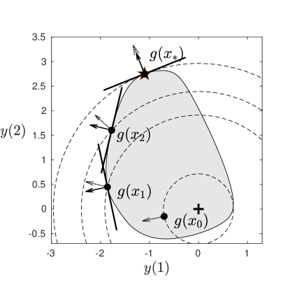
Figure 1: Illustration of the first three iterates $x_{0},x_{1},x_{2}$ by the SCF (3.1) for the mNEPv (3.16): the dark region is the joint numerical range $W(A_{1},A_{2})$; dashed lines represent contour of $\phi(y)=\|y\|^{2}/2$ with dashed arrows the gradient directions $\nabla\phi$; solid tangent lines are ‘supporting hyperplanes’ at $y_{i}=g(x_{i})$; the maximizer of (3.17) is marked as ★.

Let us discuss two direct implications of Theorem 3.1. Firstly, equation (3.12) indicates that the SCF is a successive local linearization for the optimization (3.3): At iteration $k$, we approximate the function $\phi(y)$ by a first-order expansion

$$\ell_{k}(y):=\phi(y_{k})+\nabla\phi(y_{k})^{T}(y-y_{k})$$ (3.18)

and then solve the optimization of the linear function over the joint numerical range as

$$\max_{y\in W(\mathcal{A})}\ell_{k}(y).$$ (3.19)

By dropping the constant terms in $\ell_{k}(y)$, the maximizers of (3.19) satisfies

$$\operatorname*{arg\,max}_{y\in W(\mathcal{A})}\ \ell_{k}(y)\equiv\operatorname*{arg\,max}_{y\in W(\mathcal{A})}\ \nabla\phi(y_{k})^{T}y.$$

Hence, the solution to (3.19) is exactly $y_{k+1}$ in (3.12), and we have

$$\ell_{k}(y_{k+1})=\max_{y\in W(\mathcal{A})}\ell_{k}(y).$$ (3.20)

These observations are helpful to the proof of the global convergence of the SCF as to be presented in Section 3.2.

Secondly, it is well-known that a closed convex region $\Omega$ is the intersection of all of its supporting halfspaces. One can use intersections of sampled supporting halfspaces (i.e., a polytope) to approximate $\Omega$ from outside; see, e.g., [59, Sec. 11]. Such schemes, known as outer approximation, are commonly used for finding global optimizers of convex maximization over a convex region; see, e.g., [14] for a general description and [70] for a geometric computation of numerical radius. Since the SCF generates a sequence of supporting hyperplanes of $W(\mathcal{A})$, those hyperplanes also produce outer approximations of $W(\mathcal{A})$, which allows to combine the SCF with outer approximation schemes for the global optimization of (3.3). Detailed discussion of such approach is beyond the scope of this paper.

3.2 Convergence analysis of the SCF

In this section, we show that the SCF iteration is globally convergent to an eigenvector of the mNEPv (1.1), as indicated by the visualization of the SCF in Section 3.1. Moreover, the converged eigenvector is typically a stable one and the rate of convergence is at least linear.

Let $\{x_{k}\}$ be a sequence of unit vectors. We call $x_{*}$ an (entry-wise) limit point of $\{x_{k}\}$ if

$$x_{*}=\lim_{j\to\infty}x_{k_{j}} \{x_{k_{j}}\} k_{1}<k_{2}<\cdots$$ for some subsequence indexed by . (3.21)

By the well-known Bolzano–Weierstrass theorem, a bounded sequence in $\mathbb{C}^{n}$ always has a convergent subsequence. So the sequence $\{x_{k}\}$ of unit vectors has at least one limit point $x_{*}$.

The following theorem shows the global convergence of the SCF iteration (3.1) .

Theorem 3.2.

Let $\{x_{k}\}$ be the sequence of unit vectors generated by the SCF (3.1) for the mNEPv (1.1), and let $F(x)$ be the objective function of the corresponding aMax (1.3). Then,

1. $F(x_{k+1})\geq F(x_{k})$ for $k=0,1,\dots$, with equality holds only if $x_{k}$ is an eigenvector of the mNEPv (1.1);

2. each (entry-wise) limit point $x_{*}$ of $\{x_{k}\}$ must be an eigenvector of the mNEPv (1.1), and it holds $F(x_{*})\geq F(x_{k})$ for all $k\geq 0$.

Proof.

For item (a), the monotonicity $F(x_{k+1})\geq F(x_{k})$ is a direct consequence of the convexity of $\phi$ and (3.20). Recalling (3.18) that the linearization $\ell_{k}$ of the convex function $\phi$ is always a lower supporting function of $\phi$, i.e.,

$$\ell_{k}(y)\leq\phi(y) y\in W(\mathcal{A})$$ for all ,

we have

$$F(x_{k+1})\equiv\phi(y_{k+1})\geq\ell_{k}(y_{k+1})=\max_{y\in W(\mathcal{A})}\ell_{k}(y)\geq\ell_{k}(y_{k})=\phi(y_{k})\equiv F(x_{k}),$$ (3.22)

where the third equality is by (3.20). Moreover, if the equality $F(x_{k+1})=F(x_{k})$ holds, then (3.22) implies

$$\ell_{k}(y_{k})=\max_{y\in W(\mathcal{A})}\ell_{k}(y),$$ (3.23)

namely,

$$y_{k}\in\operatorname*{arg\,max}_{y\in W(\mathcal{A})}\ell_{k}(y)\equiv\operatorname*{arg\,max}_{y\in W(\mathcal{A})}\nabla\phi(y_{k})^{T}y.$$

According to Lemma 3.1, $y_{k}=g(x_{k})$ and $x_{k}$ is an eigenvector for the largest eigenvalue of $H_{v_{k}}$ with $v_{k}=\nabla\phi(y_{k})$. Since $H_{v_{k}}\equiv H(x_{k})$, we have $H(x_{k})x_{k}=\lambda x_{k}$ and $\lambda$ is the largest eigenvalue, i.e., $x_{k}$ is an eigenvector of the mNEPv (1.1).

For item (b), let $\{x_{k_{j}}\}$ be a subsequence of $\{x_{k}\}$ convergent to $x_{*}$. The monotonicity of $F(x_{k+1})\geq F(x_{k})$ from item (a) implies $F(x_{*})\geq F(x_{k})$ for all $k\geq 0$.

To show $x_{*}$ is an eigenvector, we denote by $y_{k_{j}}=g(x_{k_{j}})$ and $y_{*}=g(x_{*})$. The linearization of $\phi$ at $y_{*}$ satisfies

$$\ell_{*}(y):=\phi(y_{*})+\nabla\phi(y_{*})^{T}(y-y_{*})=\lim_{j\to\infty}\ell_{k_{j}}(y),$$ (3.24)

where the last equality is due to $y_{*}=\lim_{j\to\infty}y_{k_{j}}$ and the continuity of $\phi$ and $\nabla\phi$ (recall $\ell_{k}$ from (3.23)).

We first show that

$$\nabla\phi(y_{*})^{T}(y-y_{*})\leq 0\quad\text{for all $y\in W(\mathcal{A})$}.$$ (3.25)

Otherwise, there exists a $\widetilde{y}\in W(\mathcal{A})$ with

$$\varepsilon:=\nabla\phi(y_{*})^{T}(\widetilde{y}-y_{*})>0.$$ (3.26)

Due to the convergence of $\ell_{k_{j}}\to\ell_{*}$ in (3.24), there exists $N\geq 0$ such that for all $j\geq N$,

$$\ell_{k_{j}}(\widetilde{y})\geq\ell_{*}(\widetilde{y})-{\varepsilon}/{2}.$$ (3.27)

It then follows from (3.22) (with $k=k_{j}$) that for all $j\geq N$,

$$\phi(y_{k_{j}+1})\geq\max_{y\in W(\mathcal{A})}\ell_{k_{j}}(y)\ \geq\ \ell_{k_{j}}(\widetilde{y})\ \geq\ \ell_{*}(\widetilde{y})-\frac{\varepsilon}{2}=\phi(y_{*})+\frac{\varepsilon}{2},$$

where the last two equations are due to (3.27) and (3.26). This implies $F(x_{k_{j}+1})\geq F(x_{*})+\varepsilon/2$, contracting $F(x_{*})\geq F(x_{k})$ for all $k$.

It follows from (3.24) and (3.25) that

$$\ell_{*}(y_{*})=\max_{y\in W(\mathcal{A})}\ell_{*}(y)=\phi(y_{*}).$$

By the same arguments as for the $y_{k}$ in (3.23), we have $x_{*}$ is an eigenvector of the mNEPv (1.1). ∎

In Section 4, we will discuss the mNEPv (1.1) arising from optimization in the form of the aMax (1.3). Then the monotonicity of the objective function is highly desirable. Starting from any $x_{0}$, the SCF will find an eigenvector $x_{*}$ that has a increased function value $F(x_{*})\geq F(x_{0})$.

Theorem 3.2 guarantees the global convergence of the SCF to an eigenvector $x_{*}$ of the mNEPv (1.1). It may happen that $x_{*}$ is a non-stable eigenvector. For example, if the initial $x_{0}$ is itself a non-stable eigenvector, or if the SCF unluckily jumps to an exact non-stable eigenvector during the iteration, then the iteration stagnates at that eigenvector. However except those special situations, the convergence to a non-stable eigenvector rarely happens in practice. This is because the SCF (3.1) is a fixed-point iteration of the mapping $\Pi$ (2.3). $\Pi$ is non-contractive at non-stable eigenvectors; see Section 2.1. By the local convergence analysis of the SCF for a general unitarily invariant NEPv (see [7, Theorem 1]), we can draw the local convergence of the SCF iteration (3.1) for the mNEPv (1.1) as stated in the following theorem.

Theorem 3.3.

Let $x_{*}$ be an eigenvector of the mNEPv (1.1) corresponding to a simple eigenvalue $\lambda_{*}$, $\mathcal{L}$ be the $\mathbb{R}$-linear operator (2.5) with respect to $x_{*}$, and $\rho(\mathcal{L})$ be the spectral radius of $\mathcal{L}$.

1. If $\rho(\mathcal{L})<1$ (i.e., $x_{*}$ is a stable eigenvector by Definition 2.1), then the SCF (3.1) is locally convergent to $x_{*}$, with an asymptotic convergence rate bounded by $\rho(\mathcal{L})$.

2. If $\rho(\mathcal{L})>1$ (i.e., $x_{*}$ is a non-stable eigenvector by Definition 2.1), then the SCF is locally divergent from $x_{*}$.

Here we recall that an iterate $x_{k}$ by the SCF (3.1) is understood as an one-dimensional subspace spanned by $x_{k}$. The local convergence and divergence of $x_{k}$ in Theorem 3.3 is measured by the vector angle $\angle(x_{*},x_{k}):=\cos^{-1}\left(|x_{*}^{H}x_{k}|\right)$.

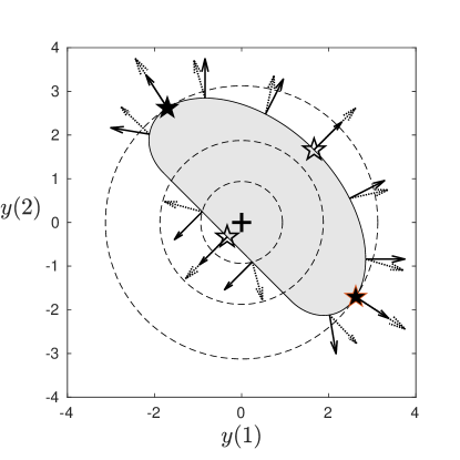
Figure 2: Illustration of stable eigenvectors, marked as solid stars ★, and non-stable eigenvectors, marked as hollow stars ☆: Close to a non-stable eigenvector, the gradients $\nabla\phi$ (dashed arrows) point away from the normal vectors (solid arrow), leading to divergence of the SCF from ☆.

By the geometric interpretation of the SCF from Theorem 3.1, we can visually illustrate its local convergence behavior revealed in Theorem 3.3. Figure 2 depicts the search directions of the SCF for the numerical radius problem described in (3.17), with the corresponding mNEPv (3.16). There are four eigenvectors (marked as stars, where the solid and dashed arrows overlap). Two solid stars are stable eigenvectors (i.e., local maximizers of (3.17)) and two hollow stars are non-stable eigenvectors (non-maximizers). The reason why the SCF is locally convergent to stable eigenvectors is now clear: Close to a solid star, the search directions $\nabla\phi(y)$ by (3.13) (dashed arrow) leads the next iteration closer to the solid star. In contrast, close to a hollow star, the search directions lead away from the hollow star. This observation also justifies the name of non-stable eigenvector, since a slight perturbation will lead the SCF to diverge from those solutions.

Combining the properties of global convergence in Theorem 3.2 and the local convergence in Theorem 3.3, we can summarize the overall convergence behavior of the SCF (3.1) as follows:

1. Let $x_{*}$ be an (entry-wise) limit point of $\{x_{k}\}$ by the SCF. Then $x_{*}$ is an eigenvector of the mNEPv (1.1); see Theorem 3.2(b).

2. The limit point $x_{*}$ is unlikely a non-stable eigenvector, since the SCF is locally divergent from non-stable eigenvectors; see Theorem 3.3(b). Consequently, the SCF is expected to converge to (at least) a weakly stable eigenvector $x_{*}$ of the mNEPv (1.1).

3. If the limit point $x_{*}$ is a stable eigenvector, then the SCF is at least locally linearly convergent to $x_{*}$; see Theorem 3.3(a).

3.3 Accelerated SCF

The iterative process (3.1) is an SCF in its simplest form, also known as the plain and pure SCF. There are a number of ways to accelerate the plain SCF, such as the damping scheme [19], level-shifting [61, 66, 78], direct inversion of iterative subspace (DIIS) with Anderson acceleration [55, 56], and preconditioned fixed-point iteration; see, e.g., [41]. Most of these schemes are originally designed for solving NEPv from electronic structure calculations. In this section, we present an acceleration scheme of the SCF (3.1) for the mNEPv (1.1).

Inverse iterations are commonly applied for linear eigenvalue problems [32] and eigenvalue-dependent nonlinear eigenvalue problems (NEP) [27]. There is an inverse iteration [33] for NEPv in the form of

$$H(x/\|x\|)\cdot x=\lambda x,$$ (3.28)

where $H(x)$ is a real symmetric matrix that is differentiable in $x\in\mathbb{R}^{n}$ [33]. For normalized $x$, we have $H(x/\|x\|)\equiv H(x)$, so that the mNEPv (1.1) can be equivalently written to an NEPv (3.28). In the following, we will first revisit the inverse iteration scheme in [33], and then propose an improved scheme for solving the mNEPv (1.1) by exploiting its underlying structure.

Let $x_{k}$ be a unit approximate eigenvector of the NEPv (3.28) and $\sigma_{k}$ be a chosen shift close to a target eigenvalue. The following inversion step is proposed in [33] to improve $x_{k}$:

$$\widetilde{x}_{k}=\alpha_{k}\left(J(x_{k})-\sigma_{k}I\right)^{-1}x_{k}\quad\text{with\quad$J(x):=\frac{\partial}{\partial x}(H(x/\|x\|)x)$},$$ (3.29)

where $\alpha_{k}$ is a normalization factor. In [33], it is shown that the iteration (3.29) is closely related to Newton’s method for the nonlinear equations $H(x/\|x\|)x-\lambda x=0$ and $x^{T}x=1$. Moreover, under mild assumptions, an inverse iteration that recursively applies (3.29) converges linearly, with a convergence factor proportional to the distance between the shift $\sigma_{k}$ and the target eigenvalue. Furthermore, a quadratic convergence is expected with the Rayleigh shift $\sigma_{k}=x_{k}^{T}H(x_{k})x_{k}$.

Directly applying the inverse iteration (3.29) to the mNEPv (1.1) will ignore the requirement that $\lambda$ is the largest eigenvalue of $H(x)$. Consequently, the process is prone to convergence to an eigenvalue that is not the largest one. Nevertheless, the rapid quadratic convergence of the inverse iteration with Rayleigh shifts is appealing. We hence propose to only use the inversion step (3.29) as an acceleration for the SCF iteration (3.1).

We first note that despite the matrix $H(x)$ of the mNEPv (1.1) is symmetric when all coefficient matrices $A_{1},\dots,A_{m}$ are real symmetric, the Jacobian $J(x)$ in (3.30) is generally not. Specifically, the Jacobian $J(x)$ of $H(x)$ is given by

$$J(x) \equiv\frac{\partial}{\partial x}(\,H(x/\|x\|)x\,)=H(x)+2M(x)C(x)M(x)^{T}P(x),$$ (3.30)

where $M(x)=[A_{1}x,\,\cdots,\,A_{m}x]$ and $C(x)=\mbox{Diag}\left(h_{1}^{\prime}\left(x^{T}A_{1}x\right),\dots,h_{m}^{\prime}\left(x^{T}A_{m}x\right)\right)$, and $P(x)=I-xx^{T}$ is a projection matrix. To symmetrize $J(x)$, we introduce

$$J_{\rm s}(x):=H(x)+2\,P(x)M(x)C(x)M(x)^{T}P(x),$$ (3.31)

and reformulate the iteration step (3.29) to

$$\widetilde{x}_{k}=\widetilde{\alpha}_{k}\cdot\left(J_{\rm s}(x_{k})-\sigma_{k}I\right)^{-1}x_{k},$$ (3.32)

where $\widetilde{\alpha}_{k}$ normalizes $\widetilde{x}_{k}$ to a unit vector. We observe that the iterations (3.29) and (3.32) are equivalent in the sense that replacing $J(x)$ by $J_{s}(x)$ in (3.29) will not affect the direction of $\widetilde{x}$. This is due to the fact that

$$J_{\rm s}(x)=J(x)+x\cdot q(x)^{T},$$

where $q(x)=2P(x)M(x)C(x)M(x)^{T}x\in\mathbb{R}^{n}$. Then by the Sherman–Morrison-Woodbury formula [30], a quick algebraic manipulation shows that

$$\left(J_{\rm s}(x_{k})-\sigma_{k}I\right)^{-1}x_{k}=c\cdot\left(J(x_{k})-\sigma_{k}I\right)^{-1}x_{k}$$

for some some constant $c$.

If the coefficient matrices $A_{1},\dots,A_{m}$ are complex Hermitian, then $H(x)$ is not holomorphically differentiable (since the diagonal entries of $H(x)$ are always real and cannot be analytic functions). In this case, the matrix $J_{\rm s}(x)$ in (3.31) no longer corresponds to the (holomorphic) Jacobian of $H(x/\|x\|)x$. Nevertheless, $J_{\rm s}(x)$ is well-defined and Hermitian (replacing all the transpose $\cdot^{T}$ to conjugate transpose $\cdot^{H}$). We can still use it for the iteration (3.32).

The SCF with an optional acceleration for solving the mNEPv (1.1) is summarized in Algorithm 1. A few remarks on the implementation detail are in order.

Algorithm 1 The SCF with optional acceleration

0:  Starting vector $x_{0}\in\mathbb{C}^{n}$, residual tolerance tol, and acceleration threshold $\mbox{tol}_{\rm acc}$.

0:  Approximate eigenpair $(\lambda_{k},x_{k})$ of the mNEPv (1.1).

1:  for $k=1,2,\dots$ do

2:      $H(x_{k-1})\,x_{k}=\lambda_{k}\cdot x_{k}$ with $\lambda_{k}=\lambda_{\max}(H(x_{k-1}))$; % SCF

3:     if $\mathrm{res}(x_{k})\leq\mbox{tol}$, then return $(\lambda_{k},x_{k})$; % test for convergence

4:     if $\mathrm{res}(x_{k})\leq\mbox{tol}_{\rm acc}$ then % acceleration if activated

5:        compute $\widetilde{x}_{k}$ by (3.32) with the shift $\sigma_{k}=x^{H}_{k}H(x_{k})x_{k}$.

6:        if $F(\widetilde{x}_{k})>F(x_{k})$, then update $x_{k}=\widetilde{x}_{k}$;

7:     end if

8:  end for

1. The initial $x_{0}$, in view of the geometry of the SCF discussed in Section 3.1, can be chosen from sampled supporting points of $W(\mathcal{A})$.

   Let $v_{i}\in\mathbb{R}^{m}$, for $i=1,\dots,\ell$, be randomly sampled search directions. We can first find the supporting points $y_{v_{i}}=g(x_{v_{i}})$ of $W(\mathcal{A})$, and then among $x_{v_{1}},\dots,x_{v_{\ell}}$, take the one with the largest value $F(x_{v_{i}})$ as the initial $x_{0}$. This greedy sampling schme increases the chance for the SCF to find the global maximizer of the aMax (1.3).

   For computation, recall Lemma 3.1 that each $x_{v_{i}}$ is an eigenvector corresponding to the largest eigenvalue of the Hermitian matrix $H_{v_{i}}$ defined in (3.10). Therefore, it requires to solve $\ell$ Hermitian eigenvalue problems for sampling $\ell$ supporting points. For efficiency, we can exploit the fact that the smallest eigenvalue of $H_{v_{i}}$ is corresponding to the largest of $H_{-v_{i}}\equiv-H(v_{i})$. Hence, we can compute two supporting points in both directions $\pm v_{i}$ by solving a single eigenvalue problem of $H_{v_{i}}$.

2. Algorithm 1 requires finding the eigenvector corresponding to the largest eigenvalue of the matrix $H(x_{k-1})$ in line 2. In addition, when the acceleration is applied, a solution of linear system with coefficient matrix $J_{\rm s}(x_{k})-\sigma_{k}I$ in line 5. For the mNEPv of small to medium sizes, direct solvers can be applied, such as QR algorithm for Hermitian eigenproblems and LU factoration for linear systems. For large sparse problems, iterative solvers are applied, e.g., the Lanczos type methods for Hermitian eigenproblems (such as MATLAB eigs), and MINRES and SYMMLQ for linear systems; see, e.g., [6, 10].

3. The acceleration with the inverse iteration is expected to work well for $x_{k}$ close to a solution. We introduced a threshold $\mbox{tol}_{\rm acc}$ to control the activation of inverse iteration in line 4. If $\mbox{tol}_{\rm acc}=0$, Algorithm 1 runs the SCF (no acceleration). If $\mbox{tol}_{\rm acc}=\infty$, Algorithm 1 applies acceleration at each step. We observe that the choice of $\mbox{tol}_{\rm acc}$ is usually not critical and $\mbox{tol}_{\rm acc}=0.1$ is used as a default value in our numerical experiments.

4. To maintain the monotonicity of $F(x_{k})$, as in the SCF, the accelerated eigenvector $\widetilde{x}_{k}$ is accepted only if $F(\widetilde{x}_{k})\geq F(x_{k})$ in line 6.

5. We use the relative residual norm

   $$\mathrm{res}(\widehat{x}):=\frac{\|H(\widehat{x})\widehat{x}-(\widehat{x}^{H}H(\widehat{x})\widehat{x})\cdot\widehat{x}\|}{\|H(\widehat{x})\|}$$ (3.33)

   to assess the accuracy of an approximate eigenvector $\widehat{x}$ in line 3, where $\|H(\widehat{x})\|$ is some convenient to evaluate matrix norm, e.g., the matrix $1$-norm as we used in the experiments.

4 Applications

The mNEPv (1.1) and the associated aMax (1.3) can be found in numerous applications. In this section, we discuss three of them. The first one is known as the quartic maximization over the Euclidean sphere and its applications for computing the numerical radius. The second one is on the best rank-one approximation of third order partial-symmetric tensors. The third is from the study of the distance to singularity of dissipative Hamiltonian differential-algebraic equation systems, or dHDAE.

4.1 Quartic maximization and numerical radius

A (homogeneous) quartic maximization over the Euclidean sphere is of the form

$$\max_{x\in\mathbb{C}^{n},\,\|x\|=1}\Big{\{}F(x):=\frac{1}{2}\sum_{i=1}^{m}\left(x^{H}A_{i}x\right)^{2}\Big{\}},$$ (4.1)

where $A_{i}$ are $n$-by-$n$ Hermitian matrices. The optimization (4.1) is a classical problem in the field of polynomial optimization, although in the literature it is usually formulated in real variables, i.e., $x\in\mathbb{R}^{n}$ with symmetric $A_{i}$ [29, 49, 84]. In addition, such problems also arise in the study of robust optimization with ellipsoid uncertainty [13]. Observe that the quartic maximization (4.1) is an aMax (1.3) with $\phi_{i}(t)=t^{2}/2$. Hence the underlying mNEPv (1.1) is of the form

$$H(x)\,x=\lambda x\quad\text{with}\quad H(x)=\sum_{i=1}^{m}(x^{H}A_{i}x)\cdot A_{i},$$ (4.2)

where the coefficient functions $h_{i}(t)=\phi_{i}^{\prime}(t)=t$ are differentiable and non-decreasing.

The most simple but non-trivial example of the quartic optimization (4.1) is $m=2$. It is the well-known problem of computing the numerical radius of a square matrix. The numerical radius of a matrix $B\in\mathbb{C}^{n\times n}$ is defined as

$$r(B):=\max_{x\in\mathbb{C}^{n},\,\|x\|=1}|x^{H}Bx|=\max_{x\in\mathbb{C}^{n},\,\|x\|=1}\Big{(}(x^{H}A_{1}x)^{2}+(x^{H}A_{2}x)^{2}\,\Big{)}^{1/2},$$ (4.3)

where $A_{1}=\frac{1}{2}(B^{H}+B)$ and $A_{2}=\frac{\imath}{2}(B^{H}-B)$, both are Hermitian matrices [30]. An extension of (4.3) is the joint numerical radius of an $m$-tuple of Hermitian matrices $\mathcal{A}=(A_{1},\dots,A_{m})$ defined as

$$r(\mathcal{A}):=\max_{x\in\mathbb{C}^{n},\,\|x\|=1}\left(\sum_{i=1}^{m}(x^{H}A_{i}x)^{2}\right)^{1/2},$$ (4.4)

see [23]. The (joint) numerical radius plays important roles in numerical analysis. For examples, the numerical radius of a matrix is applied to quantify the transient effects of discrete-time dynamical systems and analyze classical iterative methods [5, 68]. The joint numerical radius of a matrix tuple is used for studying the joint behavior of several operators; see [37] and references therein.

Numerical algorithms for computing the numerical radius of a single matrix have been extensively studied [28, 47, 48, 70, 75]. To find the global maximizer of (4.3), many methods adopt the scheme of local optimization followed by global certification. Most of those algorithms, however, do not immediately extend to computing the joint numerical radius with $m\geq 3$, and neither do they exploit the connection with the NEPv as developed in this paper. As a major benefit of the NEPv approach, it allows for fast computation of the local maximizers of the problems, so it can be used to accelerate existing approaches. Moreover, the NEPv approach provides a unified treatment for matrix tuple $\mathcal{A}$ with $m$ matrices and, hence, can serve as the basis for future development of algorithms towards the global solution of $r(\mathcal{A})$ with $m\geq 3$.

4.2 Best rank-one approximation of third order partial-symmetric tensors

Let $T\in\mathbb{R}^{n\times n\times m}$ be a third order partial-symmetric tensor, i.e., $A_{i}:=T(:,:,i)\in\mathbb{R}^{n\times n}$ is symmetric for $i=1,\dots,m$. The problem of the best rank-one partial-symmetric tensor approximation is defined by the minimization

$$\min_{\mu\in\mathbb{R},\,x\in\mathbb{R}^{n},\,z\in\mathbb{R}^{m}\atop\|x\|=1,\|z\|=1}\|T-\mu\cdot x\otimes x\otimes z\|_{F}^{2},$$ (4.5)

where $\otimes$ denotes the Kronecker product. The solution of (4.5) provides a rank-one partial-symmetric tensor $\mu_{*}\cdot x_{*}\otimes x_{*}\otimes z_{*}$ that best approximates $T$ in the Frobenius norm $\|\cdot\|_{F}$ and is also known as a truncated rank-one CP decomposition of $T$; see, e.g., [35, 84].

The best rank-one approximation (4.5) are often recast as a quartic maximization (4.1); see, e.g., [22, Eq. (6)]. Let $x_{i}$ denote the $i$-th element of a vector $x$. Then

$$\|T-\mu\cdot x\otimes x\otimes z\|_{F}^{2}=\|T\|_{F}^{2}+\mu^{2}-2\mu\sum_{i,j,k}t_{ijk}x_{i}x_{j}z_{k},$$ (4.6)

where the range of indices $i,j,k$ are omitted in the summation for clarity. Since the minimum w.r.t. $\mu$ is achieved at $\mu=\sum_{i,j,k}t_{ijk}x_{i}x_{j}z_{k}$, the best rank-one approximation (4.5) becomes the maximization

$$\max_{\|x\|=1\atop\|z\|=1}\bigg{(}\sum_{i,j,k}t_{ijk}x_{i}x_{j}z_{k}\bigg{)}^{2}=\max_{\|x\|=1\atop\|z\|=1}\bigg{(}\sum_{k}z_{k}\cdot x^{T}A_{k}x\bigg{)}^{2}=\max_{\|x\|=1}\sum_{k}\left(x^{T}A_{k}x\right)^{2},$$ (4.7)

where the first equality is by $A_{i}=T(:,:,i)$, and the second equality is due to the maximization w.r.t. $z$ is solved at

$$z=\alpha\cdot g(x)\equiv\alpha\cdot[x^{T}A_{1}x,\dots,x^{T}A_{m}x]^{T}$$ (4.8)

with $\alpha$ being a normalization factor for $\|z\|=1$ provided that $g(x)\neq 0$. The formula of $z$ in (4.8) follows from $|z^{T}g(x)|^{2}\leq\|g(x)\|^{2}$ with equality holds if $z=g(x)/\|g(x)\|$.

Problem (4.7) is a quartic maximization (4.1) with real symmetric $A_{i}$ and real variables $x\in\mathbb{R}^{n}$. By Theorem 2.1, the optimizer $x_{*}$ is an eigenvector of the mNEPv (4.2). The corresponding eigenvalue

$$\lambda_{*}=x_{*}^{T}H(x_{*})x_{*}=\sum_{k}\left(x_{*}^{T}A_{k}x_{*}\right)^{2}=\mu_{*}^{2}.$$ (4.9)

Note that any other eigenvalue $\lambda$ of (4.2) must satisfy $\lambda\equiv x^{T}H(x)x=\sum_{k}\left(x^{T}A_{k}x\right)^{2}\leq\lambda_{*}$, due to (4.9) and maximization (4.7).

The best rank-one approximation is a fundamental problem in tensor analysis; see [24, 34, 83]. Third order partial-symmetric tensors are intensively studied [21, 39, 58, 84] and found in applications such as crystal structure [22, 52], where they are termed piezoelectric-type tensors, and modeling of social networks Example 5.4. It is known that tensor rank-one approximation problems are closely related to tensor eigenvalue problems [58], such as the Z-eigenvalue [57] and $\ell^{2}$-eigenvalue [40] for general supersymmetric tensors and C-eigenvalue for third order partial-symmetric tensors [22]. Tensor eigenvalue problems provide first-order optimality conditions for the best rank-one approximation. But those eigenvalue problems are neither formulated nor studied through the lens of the NEPv as presented in this paper. Particularly, for a third order partial-symmetric tensor, its largest C-eigenvalue $\mu_{*}$ and the corresponding C-eigenvectors $(x_{*},z_{*})$ form the best rank-one approximation from (4.5); see, e.g., [22]. Whereas the tensor C-eigenvalue problem consists of two (coupled) nonlinear equations in $(\mu,x,z)$, which are fundamentally different from the mNEPv (4.2). How to efficiently solve those nonlinear equations for the C-eigenvalue is still largely open.

4.3 Distance problem in dHDAE systems

Consider the following dissipative Hamiltonian differential-algebraic equation (dHDAE):

$$J\frac{d^{j}u}{dt^{j}}=B_{0}+B_{1}\frac{du}{dt}+\cdots+B_{\ell}\frac{d^{\ell}u}{dt^{\ell}},$$ (4.10)

where $u\colon\mathbb{R}\to\mathbb{R}^{n}$ is a state function, $j$ is an integer between $0$ and $\ell$, $J=-J^{T}$ is skew symmetric, and $B_{i}\succeq 0$ are symmetric positive semi-definite for $i=0,\dots,\ell$. By convention, $\frac{d^{0}u}{dt^{0}}=u$. The dHDAE (4.10) arises in energy based modeling of dynamical systems [46, 72]. An important special case is with $j=0$ and $\ell=1$, known as the linear time-invariant dHDAE system [12, 72]. Another one is the second-order dHDAE (4.10) with $j=1$ and $\ell=2$ [12, 46].

To analyze the dynamical properties of a dHDAE system, one needs to know whether the system is close to a singular one. A dHDAE system (4.10) is called singular if $\det(P(\lambda))\equiv 0$ for all $\lambda\in\mathbb{C}$, where $P(\lambda)$ is the characteristic matrix polynomial defined by

$$P(\lambda)=-\lambda^{j}J+B_{0}+\lambda B_{1}+\cdots+\lambda^{\ell}B_{\ell}.$$ (4.11)

The distance of a dHDAE system to the closest singular dHDAE system is measured by the quantity $d_{\rm sing}(P(\lambda))$, which can be evaluated through the following optimization problem:

$$d_{\rm sing}(P(\lambda))=\min_{x\in\mathbb{R}^{n}\atop\|x\|=1}\left\{2\|Jx\|^{2}+\sum_{i=0}^{\ell}\Big{(}2\|(I-xx^{T})B_{i}x\|^{2}+(x^{T}B_{i}x)^{2}\Big{)}\right\}^{1/2},$$ (4.12)

see [46, Thm.16]. Let us show that the optimization (4.12) can be reformulated as the mNEPv (1.1). First, by the skew-symmetry of $J$ and the symmetry of $B_{i}$, we can write (4.12) as

$$\Big{(}d_{\rm sing}(P(\lambda))\Big{)}^{2} =\min_{x\in\mathbb{R}^{n}\atop\|x\|=1}\left\{2\cdot x^{T}(J^{T}J)x+\sum_{i=0}^{\ell}\left[2x^{T}(B_{i}^{T}B_{i})x-(x^{T}B_{i}x)^{2}\right]\right\}$$

$$=-2\cdot\max_{x\in\mathbb{R}^{n}\atop\|x\|=1}\left\{x^{T}A_{1}x+\frac{1}{2}\sum_{i=2}^{\ell+2}(x^{T}A_{i}x)^{2}\right\},$$ (4.13)

where $A_{1}\equiv J^{2}-\sum_{i=0}^{\ell}B_{i}^{2}$ and $A_{i}\equiv B_{i-2}$ for $i=2,\dots,\ell+2$. Consequently, (4.13) is of the form of the aMax (1.3):

$$\max_{x\in\mathbb{R}^{n},\,\|x\|=1}\Big{\{}F(x):=x^{T}A_{1}x+\frac{1}{2}\sum_{i=2}^{\ell+2}\left(x^{T}A_{i}x\right)^{2}\Big{\}},$$ (4.14)

with $\phi_{1}(t)=t$ and $\phi_{i}(t)=t^{2}/2$ for $i=2,\dots,\ell+2$. By the variational characterization in Theorem 2.1, a local maximizer of (4.14) can be found by solving the following mNEPv of the form (1.1):

$$H(x)x=\lambda x\quad\text{with}\quad H(x)\equiv A_{1}+\sum_{i=2}^{\ell+2}(x^{T}A_{i}x)\cdot A_{i}.$$ (4.15)

where $h_{1}(t)=1$ and $h_{i}(t)=t$ for $i=2,\dots,\ell+2$ are non-decreasing and differentiable functions.

There are a couple of studies on estimating the upper and lower bounds of the quantity $d_{\rm sing}(P(\lambda))$ [46, 54]. For linear systems, there is a recent work for estimating $d_{\rm sing}(P(\lambda))$ with a two-level minimization using ODE-based gradient flow [26]. The mNEPv approach provides an alternative for estimating $d_{\rm sing}(P(\lambda))$ of dHDAE systems of an arbitrary order; see Examples 5.2 and 5.3 in Section 5.

5 Numerical examples

In this section, we present numerical examples of Algorithm 1 for solving the mNEPv (1.1) arising from the applications described in Section 4. The main purpose of the experiments is to illustrate the convergence behavior of the SCF (Algorithm 1 with $\mbox{tol}_{\rm acc}=0$) and the efficiency of accelerated SCF (Algorithm 1 with $\mbox{tol}_{\rm acc}=0.1$). The error tolerance for both algorithms are set to $\mbox{tol}=10^{-13}$. All experiments are carried out in MATLAB and run on a Dell desktop with Intel i9-9900K CPU@3.6GHZ and 16GB core memory.

Example 5.1.

Consider the computation of the numerical radius for a matrix $B\in\mathbb{C}^{n\times n}$. As discussed in Section 4.1, the related mNEPv is given by (3.16) and the variational characterization is by the optimization (3.17) with Hermitian matrices $A_{1}=(B^{H}+B)/2$ and $A_{2}=(B^{H}-B)\cdot\imath/2$. For numerical experiment, we consider the following matrix

$$B=\begin{bmatrix}0.6&-0.2&-1.9&-0.3\\ -0.1&-0.3&-1.3&-1.2\\ -2.0&-1.6&-2.1&1.3\\ -0.1&-1.6&1.5&-0.1\end{bmatrix}+\imath\begin{bmatrix}0.6&2.5&-0.2&2.5\\ 2.3&-2.6&0.4&1.3\\ 0.0&0.6&-0.4&1.2\\ 2.0&1.4&1.0&-2.3\end{bmatrix}.$$ (5.1)

The corresponding numerical range $W(A_{1},A_{2})$ is depicted in the left plot of Figure 3 as the shaded region. Following the discussion in Section 3.1, we sampled $100$ different starting vectors $x_{0}$ to run the SCF, where each $y_{0}=g(x_{0})$ is a supporting point of $W(A_{1},A_{2})$, depicted in Figure 3 as dots on the boundary of $W(A_{1},A_{2})$. Recalling the discussion on the implementation of Algorithm 1, such initial iterates $x_{0}$ can be obtained from the eigenvectors $x_{v}$ of the matrix $H_{v}$ for sampled directions $v\in\mathbb{R}^{2}$ (see Lemma 3.1 and Section 3.3). Note that we can represent a unit direction $v\in\mathbb{R}^{2}$ by polar coordinates as $v=[\cos\theta,\sin\theta]^{T}$ with $\theta\in[0,2\pi)$. The initial vectors $x_{0}$ are set as

$$x_{0}:=x_{v}\quad\text{with $v=[\cos\theta,\sin\theta]^{T}$},$$ (5.2)

using $100$ equally distant $\theta$ between $0$ and $2\pi$. The sampled $g(x_{0})$ are well distributed on the boundary of $W(A_{1},A_{2})$, as shown in Figure 3.

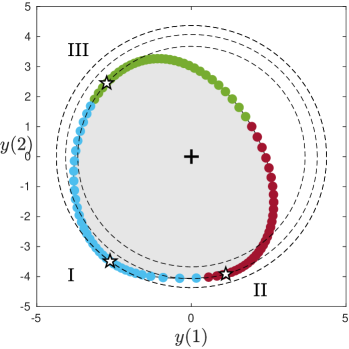
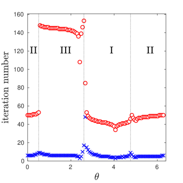
Figure 3: Left: Numerical range $W(A_{1},A_{2})$ of the matrix in (5.1), where ☆ represent the solution for the mNEPv and $\bullet$ the starting $g(x_{0})$ of the SCF; The $\bullet$ are colored according to the solution they have computed (blue is for solution I, red for II, and green for III); The dashed are contours of $\phi(y)=2^{-1}\|y\|_{2}^{2}$; see (3.17). Right: Number of iterations by the SCF (marked ‘o’) and accelerated SCF (marked ‘$\times$’) for different starting $x_{0}$, parameterized by $\theta\in[0,2\pi)$ as in (5.2).

For $100$ runs of the SCF, three different solutions are found. In Figure 3, they are labeled respectively with I, II, III, in descending order of their objective values of (3.17). The initial $g(x_{0})$ on the boundary of $W(A_{1},A_{2})$ are colored the same if SCF will converge to the same solution, which, hence, reveals the region of convergence for SCF. The numbers of SCF iterations with each $x_{0}$ are reported in the right plot of Figure 3. We can see that the iterations are determined by the eigenvector SCF computed, and they stay almost flat for that eigenvector. For the SCF, the iteration numbers vary for different solution. Whereas for the accelerated SCF, they are almost independent of the choice of the initial $x_{0}$, with only a moderate increase on the boundary of two convergence regions.

The left plot of Figure 4 depicts the convergence history of the objective function $F(x_{k})$ for four different starting vectors $x_{0}$, corresponding to the equally distant $\theta\in\{0,\,\pi/2,\,\pi,\,3\pi/2\}$ from Figure 3. As expected the SCF demonstrates monotonic convergence. The right plot in Figure 4 shows the relative residual norms of $(\lambda_{k},x_{k})$ as defined in (3.33). We can see that the SCF quickly enters the region of linear convergence in all cases (in about 3 iterations). The acceleration takes full advantage of the rapid initial convergence and speeds up the SCF significantly. We note that in this example the matrices $A_{1}$ and $A_{2}$ are complex Hermitian. The inverse iteration (3.32) with Rayleigh shift $\sigma_{k}$ is not guaranteed quadratically convergent.

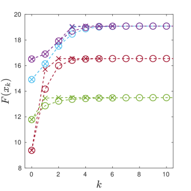
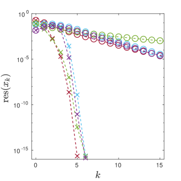
Figure 4: Example 5.1. Left: Convergence history of $F(x_{k})$ by the SCF (marked ‘o’) and accelerated SCF (marked ‘$\times$’), where each colored curve is a run with a particular $x_{0}$ from $4$ different starting vectors. Right: Relative residual norms (3.33).

Example 5.2.

We consider the mNEPv (4.15) arising in the distance problem of dHDAE systems described in Section 4.3. The characteristic polynomial of a linear dHDAE system is given by

$$P(\lambda):=-J+R+\lambda E,$$ (5.3)

where $J=-J^{T}$ is a skew symmetric, and $E$ and $R$ are symmetric positive definite matrices. As discussed in Section 4.3, the computation of distance to singularity $d_{\rm sing}(P(\lambda))$ leads to the optimization (4.13) and the associated mNEPv (4.15), where

$$F(x)=x^{T}A_{1}x+\frac{1}{2}\sum_{i=2}^{3}(x^{T}A_{i}x)^{2}\quad\mbox{and}\quad H(x)=A_{1}+\sum_{i=2}^{3}(x^{T}A_{i}x)\cdot A_{i},$$ (5.4)

and $A_{1}=J^{2}-E^{2}-R^{2}$, $A_{2}=E$ and $A_{3}=R$.

For numerical experiments, the matrices $\{J,R,E\}$ of order 30 are generated randomly. Similar to Example 5.1, the initial vectors $x_{0}$ of the SCF are computed from supporting points of the joint numerical range $W(A_{1},A_{2},A_{3})\subset\mathbb{R}^{3}$ along several sampled direction $v\in\mathbb{R}^{3}$. Here, recall that a unit $v\in\mathbb{R}^{3}$ can be represented by spherical coordinates as

$$v=[\sin\eta\cos\theta,\,\sin\eta\sin\theta,\,\cos\eta]^{T}\quad\text{with $\eta\in[0,2)$ and $\theta\in[0,2\pi)$}.$$ (5.5)

We have therefore constructed an equispaced grid of $20$-by-$40$ points of $(\eta,\theta)\in[0,\pi]\times[0,2\pi]$, yielding $800$ supporting points of $W(A_{1},A_{2},A_{3})$. They are depicted in the left plot of Figure 5, together with the approximate numerical range $W(A_{1},A_{2},A_{3})$ they generate.

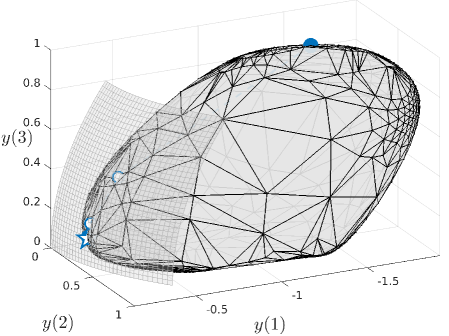
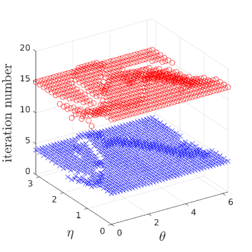
Figure 5: Left: Approximate numerical range $W(A_{1},A_{2},A_{3})$, based on $800$ sample supporting points on the boundary (nodes of the mesh); The ☆ represents the solution for the mNEPv, $\bullet$ the starting $g(x_{0})$, and ‘$\circ$’ the first few supporting points $g(x_{k})$ by SCF; The smaller mesh that crosses ☆ is part of the level-surface $\phi(y)=\phi(y_{*})$ for $\phi(y)=y(1)+(y(2)^{2}+y(3)^{2})/2$ at the solution $y_{*}=g(\widehat{x}_{*})$. Right: Number of iterations by the SCF (marked ‘o’) and the accelerated SCF (marked ‘$\times$’) for different starting $x_{0}$, parameterized by $\theta\in[0,2\pi)$ and $\eta\in[0,\pi)$ as in (5.5).

From all $800$ initial $x_{0}$, the SCF converge to a same solution, as marked in the left plot of Figure 5. This solution appears to be the global optimizer of the optimization (4.13), as visually verified by the level-surface of the objective function $\phi(y)$ for the corresponding optimization over the joint numerical range (3.3). From the numbers of iterations reported in the right plot of Figure 5, we can see that both SCF and accelerated SCF converge rapidly to the solution. The iteration numbers are not sensitive to the choice of initial vectors.

Figure 6 depicts the convergence history of $F(x_{k})$ and the relative residual norms by the SCF from six different starting vectors $x_{0}$ (sampled supporting points of $W(A_{1},A_{2},A_{2})$ along the three coordinate axes). We observe that the SCF with different starting vector converges monotonically to the same solution. The accelerated SCF greatly reduces the number of iterations and shows the quadratic convergence rate.

Figure 6: Left: Convergence history of $F(x_{k})$ by the SCF (marked ‘o’) and accelerated SCF (marked ‘$\times$’), where each colored curve is a run with a particular $x_{0}$ from $6$ different starting vectors. Right: Relative residual norms (3.33).

Recall that a computed $\widehat{x}_{*}$ may not be a global maximizer of the aMax (4.13). But we have at least an upper bound of the distance:

$$d_{\rm sing}(P(\lambda))\equiv\big{(}-2\cdot\max_{\|x\|=1}F(x)\big{)}^{1/2}\leq\big{(}-2\cdot F(\widehat{x}_{*})\big{)}^{1/2}.$$ (5.6)

If the initial vector $x_{0}$ of the SCF is especially set to be the eigenvector corresponding to the largest eigenvalue of $A_{1}$, then we have

$$\big{(}-2\cdot F(\widehat{x}_{*})\big{)}^{1/2}\leq\big{(}-2\cdot F(x_{0})\big{)}^{1/2}\leq\delta_{M}:=\big{(}-2\cdot\lambda_{\max}(A_{1})\big{)}^{1/2},$$ (5.7)

where the first inequality is by the monotonicity of the SCF (see Theorem 3.2) and the second inequality is by the definition of $F(x)$ (5.4) (recall that $R$ and $E$ are positive definite). The quantity $\delta_{M}$ was introduced in [46, Thms.13 and 16] and used as an estimation of the quantity $d_{\rm sing}(P(\lambda))$. It follows from the inequalities (5.6) and (5.7) that the SCF always produces a sharper upper bound of $d_{\rm sing}(P(\lambda))$. For example, in a numerical example, the SCF provides an estimation $\big{(}-2\cdot F(\widehat{x}_{*})\big{)}^{1/2}\approx 0.5989$. In contrast, $\delta_{M}\approx 0.6923$.

We note that the quantity $\delta_{M}$ has been revisited in a recent work [54], where a computable upper bound was proposed. The latter, however, involves a more complicated optimization of sum of generalized Rayleigh quotients and does not ensure a better estimation than $\delta_{M}$; see [54, Thm. 3.7 and Example 3]. In another related work [26], the authors considered an approach to estimate $d_{\rm sing}(P(\lambda))$, based on the observation that $d_{\rm sing}(P(\lambda))$ is the smallest root of a monotonically decreasing function $w$. A root finding method such as the bisection can be applied. The difficulty there lies in the evaluation of the function $w$. For a given $\epsilon$, evaluating $w(\epsilon)$ can be very expensive as it requires the solution of an optimization by a gradient flow method, which involves repeated solution of Hermitian eigenvalue problems of size $n$.

Example 5.3.

In this example, we consider a quadratic dHDAE system with a characteristic polynomial

$$P(\lambda):=-\lambda G+K+\lambda D+\lambda^{2}M,$$

where $G=-G^{T}$ is skew symmetric, and $M$, $D$ and $K$ are symmetric positive definite. By Section 4.3, the computation of distance to singularity $d_{\rm sing}(P(\lambda))$ leads to the optimization (4.13) and the mNEPv (4.15), where

$$F(x)=x^{T}A_{1}x+\frac{1}{2}\sum_{i=2}^{4}(x^{T}A_{i}x)^{2}\quad\mbox{and}\quad H(x)=A_{1}+\sum_{i=2}^{4}(x^{T}A_{i}x)\cdot A_{i},$$

where $A_{1}=G^{2}-M^{2}-D^{2}-K^{2}$, $A_{2}=M$, $A_{3}=D$, and $A_{4}=K$.

For numerical experiments, we consider a lumped-parameter mass-spring-damper system, $M\ddot{u}+D\dot{u}+Ku=f$; see, e.g., [73], with $n$ point-masses and $n$ spring-damper pairs. The matrices $D$ and $K$ are interchangeable with $DK=KD$ and are simultaneously diagonalizable. We pick a random skew symmetric $G$ as in Section 4.1 to simulate the gyroscopic effect. The sizes $n$ of the matrices are set ranging from $500$ to $3000$. For each set of testing matrices, we apply the SCF with $100$ different starting vectors $x_{0}$. Again, those $x_{0}$ are computed from supporting points of the joint-numerical range $W(\mathcal{A})\subset\mathbb{R}^{4}$ along $100$ randomly sampled directions $v\in\mathbb{R}^{4}$.

Similar to the linear system in Example 5.2, the SCF always converge to a same solution from all $100$ different starting vectors. The convergence history of the SCF and the accelerated SCF for a case of $n=1000$, with $8$ randomly selected starting vectors are depicted in Figure 7. It shows a same convergence behavior of the SCF and accelerated SCF as in the previous example.

Figure 7: Left: Convergence history of $F(x_{k})$ by the SCF (marked ‘o’) and accelerated SCF (marked ‘$\times$’), where each colored curve is a run with a particular $x_{0}$ from $8$ different starting vectors (lines overlapped). Right: Relative residual norms (3.33).

Table 1 summarizes the iteration number and computation time for the algorithms from all testing cases. We can see that the performance of both SCF and accelerated SCF are not much affected by the choice of initial vectors. Both algorithms converge rapidly, and the accelerated SCF speed up to a factor between $2.5$ to $6.2$.

Table 1: Number of iterations and computation time (in seconds) for various problem sizes $n$. Reported are average results from $100$ runs with different starting vectors, with the largest deviations also marked.

$n$	algorithms	iterations	timing	speedup
$500$	SCF	$17.0$ ($\pm 4.0$)	$1.18$ ($\pm 0.34$)	–
	accel. SCF	$5.3$ ($\pm 1.3$)	$0.34$ ($\pm 0.14$)	$2.9$ to $4.5$
$1000$	SCF	$21.3$ ($\pm 3.3$)	$6.54$ ($\pm 1.15$)	–
	accel. SCF	$4.7$ ($\pm 1.3$)	$1.32$ ($\pm 0.48$)	$3.9$ to $6.2$
$2000$	SCF	$17.0$ ($\pm 4.0$)	$4.91$ ($\pm 1.58$)	–
	accel. SCF	$4.8$ ($\pm 1.8$)	$1.52$ ($\pm 0.73$)	$2.5$ to $4.9$
$3000$	SCF	$16.9$ ($\pm 3.9$)	$20.51$ ($\pm 5.33$)	–
	accel. SCF	$5.2$ ($\pm 1.2$)	$6.39$ ($\pm 1.93$)	$2.7$ to $4.0$

Example 5.4.

As discussed in Section 4.2, the problem of best rank-one approximation for a partial-symmetric tensor $T\in\mathbb{R}^{n\times n\times m}$ leads to a quartic optimization (4.7) and the corresponding mNEPv (4.2), where the coefficient matrices are $A_{i}:=T(:,:,i)\in\mathbb{R}^{n\times n}$ for $i=1,\dots,m$.

For non-negative tensors, the objective function $F(x)$ of (4.7) satisfies $F(|x|)\geq F(x)$, where $|\cdot|$ denotes componentwise absolute value. Therefore, it is advisable to start the SCF (3.1) with a non-negative initial $x_{0}$. Note that if $x_{k}\geq 0$ then $H(x_{k})\geq 0$. By the Perron-Frobenius theorem [30], the eigenvector $x_{k+1}$ corresponding to the largest eigenvalue of $H(x_{k})$ is also non-negative. This implies that the subsequent iterates $x_{k}$ by the SCF will remain non-negative.

We note that for a non-negative tensor $T$ and a non-negative initial $x_{0}$, the SCF (3.1) is indeed equivalent to the Alternating Least Squares (ALS) algorithm for finding the best rank-one approximation (4.5). Recall that in Section 4.2, the best rank-one approximation (4.5) is turned into the maximization problem:

$$\max_{\|x\|=1,\,\|z\|=1}\left(z^{T}\cdot g(x)\right)^{2},$$ (5.8)

where $g(x)=[x^{T}A_{1}x,\ldots,x^{T}A_{m}x]^{T}$. Maximizing alternatively with respect to $z$ and $x$ leads to the alternating iteration:

$$\left\{\begin{aligned} z_{k+1}&=\operatorname*{arg\,max}_{\|z\|=1}\left(z^{T}\cdot g(x_{k})\right)^{2}=\alpha_{k}\cdot g(x_{k}),\\ x_{k+1}&=\operatorname*{arg\,max}_{\|x\|=1}\left(z_{k+1}^{T}\cdot g(x)\right)^{2}=\operatorname*{arg\,max}_{\|x\|=1}\left(x^{T}\cdot H(x_{k})\cdot x\right)^{2},\end{aligned}\right.$$ (5.9)

for $k=1,2,3,\dots$, where $\alpha_{k}>0$ is a normalization factor for $z_{k+1}$. Recall that $H(x_{k})\geq 0$ if $x_{k}\geq 0$. The maximizer $x_{k+1}$ of (5.9) is the eigenvector corresponding to the largest eigenvalue of $H(x_{k})$, i.e., $H(x_{k})x_{k+1}=\lambda_{\max}\cdot x_{k+1}$, due to the Perron-Frobenius theorem. Therefore (5.9) coincides with the SCF. The ALS algorithms are commonly used for low-rank approximations in tensor computations [35]. The scheme (5.9) accounts for the partial symmetry of the rank-one tensor $\lambda\cdot x\otimes x\otimes z$ such that only two vectors $x$ and $z$ are alternated.

In Algorithm 1, we use MATLAB eigs for solving the eigenvalue computation and minres for solving the linear system in the acceleration (3.32). We use an adaptive error tolerance $\mbox{Tol}=\min\{10^{-3},\mbox{res}(x_{k})^{2}\}$ for each call of eigs and minres.

For numerical experiments, we use the following thrid order partial-symmetric tensors.

1. The New Orleans tensor , created from the Facebook New Orleans network. The original data contains a list of all of the user-to-user links (undirected) and a timestamp for the establishment of the link. The links are collected on a monthly (30 day) basis for $20$ months, with each month corresponding to a slice of $T(:,:,i)$. The size of the resulting tensor $T$ is $63891\times 63891\times 20$ with $477778$ nonzeros.

2. The Princeton tensor , created from a Facebook ‘friendship’ network at Princeton, following the setting up in [25]. The element $T(i,j,k)=1$ if students $i$ and $j$ are friends and one of them has a status flag $k$. The size of the resulting tensor $T$ is $6593\times 6593\times 6$ with $70248$ nonzeros.

3. The Reuters tensor , created from a news network based on all stories released by the news agency Reuters, concerning the September 11 attack during the 66 consecutive days beginning at September 11, 2001. The vertices of the network are words, and there is an edge between two words if they appear in the same sentence, with the weight of an edge being the frequency. The size of the tensor $T$ is $13332\times 13332\times 66$ with $486894$ nonzeros.

All three tensors are non-negative and sparse (density $\approx 10^{-5}$), so are the corresponding coefficient matrices $A_{i}=T(:,:,i)$ for $i=1,\dots,m$. We use $100$ randomly generated and non-negative starting vectors $x_{0}$ to run the SCF (using x0=abs(randn(n,1))). The convergence history is reported in Figure 8. We observe that from different starting vectors,  Algorithm 1 always converge to the same solution and the convergence rate appears not affected by the choice of starting vectors. Also, the accelerated SCF significantly reduces the number of the SCF iterations and has a quadratic convergence rate.

The computed optimal values of the objective function and timing of the ALS (i.e., the SCF) and the accelerated SCF are reported in Table 2. The accelerated SCF speeds up the ALS by a factor of 2. This demonstrates one of the benefits of the NEPv reformulation for allowing the development of effective acceleration scheme of the ALS.

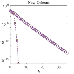
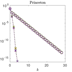
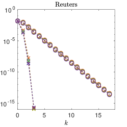
Figure 8: Convergence history of relative residual norms $\mbox{res}(x_{k})$ (3.33) by the SCF (‘$\circ$’) and accelerated SCF (‘$\times$’). Each colored curve represents a run with a different starting vector from $100$ randomly generated $x_{0}\geq 0$ (lines overlapped).

Table 2: Objective function value $F(x_{*})$ of the computed eigenvectors $x_{*}$, total iteration number, and computation time (in seconds). Reported are average results from $100$ runs with different starting vectors, with the largest deviations also marked.

tensor	algorithms	$F(x_{*})$	iterations	timing
New Orleans	ALS	$257.1509714238355$ ($\pm 3\cdot 10^{-13}$)	$36$	$1.69$ ($\pm 2\cdot 10^{-1}$)
	accel. SCF	$257.1509714238355$ ($\pm 3\cdot 10^{-13}$)	6	$0.75$ ($\pm 1\cdot 10^{-1}$)
Princeton	ALS	$26441.19404229125$ ($\pm 3\cdot 10^{-11}$)	$30$	$0.42$ ($\pm 4\cdot 10^{-2}$)
	accel. SCF	$26441.19404229123$ ($\pm 2\cdot 10^{-12}$)	$5$	$0.18$ ($\pm 5\cdot 10^{-2}$)
Reuters	ALS	$118777.1084768529$ ($\pm 1\cdot 10^{-10}$)	$18$	$0.65$ ($\pm 4\cdot 10^{-2}$)
	accel. SCF	$118777.1084768529$ ($\pm 1\cdot 10^{-10}$)	$4$	$0.32$ ($\pm 2\cdot 10^{-2}$)

6 Concluding remarks

We investigated the mNEPv (1.1). A variational characterization for the mNEPv is revealed. Based on the variational characterization, we provided a geometric interpretation of the SCF iterations for solving the mNEPv. The geometry of the SCF illustrates the global monotonic convergence of the algorithm and leads to a rigorous proof of the global convergence of the SCF. In addition, we presented an inverse-iteration based scheme to accelerate the convergence of the SCF. Numerical examples demonstrated the effectiveness of the accelerated SCF for solving the mNEPv arising from different applications. By the intrinsic connection between the mNEPv (1.1) and the aMax (1.3), we developed an NEPv approach for solving the aMax. Algorithmically, it allows the use of state-of-the-art eigensolvers for fast solution of the aMax.

Most results presented in this work can be extended to the case NEPv (1.1) with $h_{i}$ being non-decreasing and locally Lipschitz continuous, i.e.,

$$c_{i}(t):=\limsup_{t+\delta t\in[\ell_{i},u_{i}]\atop\delta t\to 0}\frac{h_{i}(t+\delta t)-h_{i}(t)}{\delta t}<\infty$$ (6.1)

for all $t\in[\ell_{i},u_{i}]$ with $\ell_{i}=\lambda_{\min}(A_{i})$, $u_{i}=\lambda_{\max}(A_{i})$, and $i=1,\dots,m$. For example, in complete analogy to Theorem 2.1, it is possible to establish a variational characterization of such NEPv. In addition, we expect this work to serve as the basis for the study of a more general class of NEPv in the form of

$$H(x)x=\lambda x\quad\text{with}\quad H(x)=\sum_{i=1}^{m}h_{i}(g(x))A_{i},$$ (6.2)

with an $m$-tuple of Hermitian matrices $\mathcal{A}=(A_{1},\dots,A_{m})$, $g$ by (3.2), and $h_{i}:\mathbb{R}^{m}\to\mathbb{R}$ to be given functions. Similar to the mNEPv (1.1), one can expect to establish variational characterizations of (6.2), at least for particular functions of $h_{i}$. How to extend the theoretical analysis and geometric interpretation of the SCF to a general NEPv (6.2) is left to future research.

References

- [1] P. A. Absil, R. Mahony, and R. Sepulchre. Optimization Algorithms on Matrix Manifolds. Princeton University Press, 2009.
- [2] H. Amann. Fixed point equations and nonlinear eigenvalue problems in ordered Banach spaces. SIAM Review, 18(4):620–709, 1976.
- [3] Y.-H. Au-Yeung and N.-K. Tsing. An extension of the Hausdorff-Toeplitz theorem on the numerical range. Proceedings of the American Mathematical Society, 89(2):215–218, 1983.
- [4] Y.-H. Au-yeung and N.-K. Tsing. Some theorems on the generalized numerical ranges. Linear Multilinear Algebra, 15(1):3–11, 1984.
- [5] O. Axelsson. Iterative Solution Methods. Cambridge University Press, 1996.
- [6] Z. Bai, J. Demmel, J. Dongarra, A. Ruhe, and H. van der Vorst. Templates for the Solution of Algebraic Eigenvalue Problems: a Practical Guide. SIAM, 2000.
- [7] Z. Bai, R.-C. Li, and D. Lu. Sharp estimation of convergence rate for self-consistent field iteration to solve eigenvector-dependent nonlinear eigenvalue problems. SIAM J. Matrix Anal. Appl., 43(1):301–327, 2022.
- [8] Z. Bai, D. Lu, and B. Vandereycken. Robust Rayleigh quotient minimization and nonlinear eigenvalue problems. SIAM J. Sci. Comput, 40(5):A3495–A3522, 2018.
- [9] W. Bao and Q. Du. Computing the ground state solution of Bose–Einstein condensates by a normalized gradient flow. SIAM J. Sci. Comput., 25(5):1674–1697, 2004.
- [10] R. Barrett, M. Berry, T. F. Chan, J. Demmel, J. Donato, J. Dongarra, V. Eijkhout, R. Pozo, C. Romine, and H. Van der Vorst. Templates for the Solution of Linear Systems: Building Blocks for Iterative Methods. SIAM, 1994.
- [11] V. Batagelj and A. Mrvar. A density based approaches to network analysis: Analysis of Reuters terror news network. In Proceedings of the 9th Annual ACM SIGKDD, 2003.
- [12] C. Beattie, V. Mehrmann, H. Xu, and H. Zwart. Linear port-Hamiltonian descriptor systems. Math. Control Signals Syst., 30(4):1–27, 2018.
- [13] A. Ben-Tal and A. Nemirovski. Robust convex optimization. Math. Opera. Res., 23(4):769–805, 1998.
- [14] H. P. Benson. Concave minimization: theory, applications and algorithms. In Handbook of Global Optimization, pages 43–148. Springer, 1995.
- [15] V. Berinde. Iterative Approximation of Fixed Points. Springer Berlin, Heidelberg, 2007.
- [16] R. Bhatia. Matrix Analysis. Springer New York, NY, 2013.
- [17] Y. Cai, L.-H. Zhang, Z. Bai, and R.-C. Li. On an eigenvector-dependent nonlinear eigenvalue problem. SIAM J. Matrix Anal. Appl., 39(3):1360–1382, 2018.
- [18] E. Cancès, G. Kemlin, and A. Levitt. Convergence analysis of direct minimization and self-consistent iterations. SIAM J. Matrix Anal. Appl., 42(1):243–274, 2021.
- [19] E. Cancès and C. Le Bris. Can we outperform the DIIS approach for electronic structure calculations? Int. J. Quantum Chem., 79(2):82–90, 2000.
- [20] E. Cancès and C. Le Bris. On the convergence of SCF algorithms for the Hartree–Fock equations. ESAIM: Mathematical Modelling and Numerical Analysis, 34(4):749–774, 2000.
- [21] J. D. Carroll and J.-J. Chang. Analysis of individual differences in multidimensional scaling via an N-way generalization of “Eckart-Young” decomposition. Psychometrika, 35(3):283–319, 1970.
- [22] Y. Chen, A. Jákli, and L. Qi. The C-eigenvalue of third order tensors and its application in crystals. J. Ind. Manag. Optim., 2021.
- [23] M. Chō and M. Takaguchi. Boundary points of joint numerical ranges. Pac. J. Math., 95(1):27–35, 1981.
- [24] L. De Lathauwer, B. De Moor, and J. Vandewalle. A multilinear singular value decomposition. SIAM J Matrix Anal. Appl., 21(4):1253–1278, 2000.
- [25] L. Eldén and M. Dehghan. A Krylov-Schur like method for computing the best rank- approximation of large and sparse tensors. Numer. Algor., pages 1–33, 2022.
- [26] N. Guglielmi and V. Mehrmann. Computation of the nearest structured matrix triplet with common null space. Electron. Trans. Numer. Anal., 55:508–531, 2022.
- [27] S. Güttel and F. Tisseur. The nonlinear eigenvalue problem. Acta Numerica, 26:1–94, 2017.
- [28] C. He and G.A. Watson. An algorithm for computing the numerical radius. IMA J. Numer. Anal., 17(3):329–342, 1997.
- [29] S. He, Z. Li, and S. Zhang. Approximation algorithms for homogeneous polynomial optimization with quadratic constraints. Math. Program., 125(2):353–383, 2010.
- [30] R. A. Horn and C. R. Johnson. Matrix Analysis. Cambridge University Press, 2012.
- [31] P. Huang, Q. Yang, and Y. Yang. Finding the global optimum of a class of quartic minimization problem. Comput. Optim. Appl., 81:923–954, 2022.
- [32] I. C. F. Ipsen. Computing an eigenvector with inverse iteration. SIAM Review, 39(2):254–291, 1997.
- [33] E. Jarlebring, S. Kvaal, and W. Michiels. An inverse iteration method for eigenvalue problems with eigenvector nonlinearities. SIAM J. Sci. Comput., 36(4):A1978–A2001, 2014.
- [34] E. Kofidis and P. A. Regalia. On the best rank-1 approximation of higher-order supersymmetric tensors. SIAM J. Matrix Anal. Appl., 23(3):863–884, 2002.
- [35] T. G. Kolda and B. W. Bader. Tensor decompositions and applications. SIAM Review, 51(3):455–500, 2009.
- [36] J. Lampe and H. Voss. A survey on variational characterization for nonlinear eigenvalue problems. Electron. Trans. Numer. Anal., 55:1–75, 2022.
- [37] C.-K. Li and E. Poon. Maps preserving the joint numerical radius distance of operators. Linear Algebra Appl., 437(5):1194–1204, 2012.
- [38] C.-K. Li and Y.-T. Poon. Convexity of the joint numerical range. SIAM J. Matrix Anal. Appl., 21(2):668–678, 2000.
- [39] N. Li, C. Navasca, and C. Glenn. Iterative methods for symmetric outer product tensor decomposition. Electron. Trans. Numer. Anal., 44:124–139, 2015.
- [40] L.-H. Lim. Singular values and eigenvalues of tensors: a variational approach. In 1st IEEE International Workshop on Computational Advances in Multi-Sensor Adaptive Processing, 2005., pages 129–132. IEEE, 2005.
- [41] L. Lin and C. Yang. Elliptic preconditioner for accelerating the self-consistent field iteration in Kohn–Sham density functional theory. SIAM J. Sci. Comput., 35(5):S277–S298, 2013.
- [42] X. Liu, X. Wang, Z. Wen, and Y. Yuan. On the convergence of the self-consistent field iteration in Kohn-Sham density functional theory. SIAM J. Matrix Anal. Appl., 35(2):546–558, 2014.
- [43] X. Liu, Z. Wen, X. Wang, and Y. Ulbrich, M. Yuan. On the analysis of the discretized Kohn-Sham density functional theory. SIAM J. Numer. Anal., 53(4):1758–1785, 2015.
- [44] D. Lu. Nonlinear eigenvector methods for convex minimization over the numerical range. SIAM J. Matrix Anal. Appl., 41(4):1771–1796, 2020.
- [45] R. M. Martin. Electronic Structure: Basic Theory and Practical Methods. Cambridge University Press, 2004.
- [46] C. Mehl, V. Mehrmann, and M. Wojtylak. Distance problems for dissipative Hamiltonian systems and related matrix polynomials. Linear Algebra Appl., 623:335–366, 2021.
- [47] E. Mengi and M. L. Overton. Algorithms for the computation of the pseudospectral radius and the numerical radius of a matrix. IMA J. Numer. Anal., 25(4):648–669, 2005.
- [48] T. Mitchell. Convergence rate analysis and improved iterations for numerical radius computation. Preprint arXiv:2002.00080, 2020.
- [49] Y. Nesterov. Random walk in a simplex and quadratic optimization over convex polytopes. Technical report, CORE Discussion Paper, UCL, Louvain-la-Neuve, Belgium, 2003.
- [50] T. T. Ngo, M. Bellalij, and Y. Saad. The trace ratio optimization problem. SIAM Review, 54(3):545–569, 2012.
- [51] J. Nocedal and S. Wright. Numerical Optimization. Springer New York, NY, 2006.
- [52] J. F. Nye. Physical Properties of Crystals: Their Representation by Tensors and Matrices. Oxford University Press, 1985.
- [53] B. N. Parlett. The Symmetric Eigenvalue Problem. SIAM, 1998.
- [54] A. Prajapati and P. Sharma. Estimation of structured distances to singularity for matrix pencils with symmetry structures: A linear algebra–based approach. SIAM J. Matrix Anal. Appl., 43(2):740–763, 2022.
- [55] P. Pulay. Convergence acceleration of iterative sequences. the case of SCF iteration. Chem. Phys. Lett., 73(2):393–398, 1980.
- [56] P. Pulay. Improved SCF convergence acceleration. J. Comput. Chem., 3(4):556–560, 1982.
- [57] L. Qi. Eigenvalues of a real supersymmetric tensor. J. Symb. Comput., 40(6):1302–1324, 2005.
- [58] L. Qi, H. Chen, and Y. Chen. Tensor Eigenvalues and Their Applications, volume 39. Springer, 2018.
- [59] R. T. Rockafellar. Convex Analysis. Princeton University Press, 2015.
- [60] C. C. J. Roothaan. New developments in molecular orbital theory. Reviews of modern physics, 23(2):69, 1951.
- [61] V.R. Saunders and I.H. Hillier. A Level–Shifting method for converging closed shell Hartree–Fock wave functions. Int. J. Quantum Chem., 7(4):699–705, 1973.
- [62] R. E. Stanton. Intrinsic convergence in closed-shell SCF calculations. A general criterion. J. Chem. Phys., 75(11):5416–5422, 1981.
- [63] G. W. Stewart and J.-G. Sun. Matrix Perturbation Theory. Academic Press, Boston, 1990.
- [64] A. Szabo and N. S. Ostlund. Modern Quantum Chemistry: Introduction To Advanced Electronic Structure Theory. Courier Corporation, 2012.
- [65] Bühler T. and M. Hein. Spectral clustering based on the graph p-Laplacian. In Proceedings of the 26th Inter. Conf. on Machine Learning, pages 81–88, 2009.
- [66] L. Thøgersen, J. Olsen, D. Yeager, P. Jørgensen, P. Sałek, and T. Helgaker. The trust-region self-consistent field method: Towards a black-box optimization in Hartree–Fock and Kohn–Sham theories. J Chem. Phys., 121(1):16–27, 2004.
- [67] A. L. Traud, P. J. Mucha, and M. A. Porter. Social structure of Facebook networks. Physica A, 391(16):4165–4180, 2012.
- [68] L. N. Trefethen and M. Embree. Spectra and Pseudospectra: the Behavior of Nonnormal Matrices and Operators. Princeton University Press, 2005.
- [69] F. Tudisco and D. J. Higham. A nonlinear spectreal method for core-periphery detection in networks. SIAM J. Math. Data Sci., 1(2):269–292, 2019.
- [70] F. Uhlig. Geometric computation of the numerical radius of a matrix. Numer. Algor., 52(3):335, 2009.
- [71] P. Upadhyaya, E. Jarlebring, and E. H. Rubensson. A density matrix approach to the convergence of the self-consistent field iteration. Numer. Algebra, Control. Optim., 11(1):99–115, 2021.
- [72] A. Van Der Schaft and D. Jeltsema. Port-Hamiltonian systems theory: An introductory overview. Found. Trends Syst. Control, 1(2-3):173–378, 2014.
- [73] K. Veselić. Damped Oscillations of Linear Systems: a Mathematical Introduction, volume 2023. Springer Berlin, Heidelberg, 2011.
- [74] B. Viswanath, A. Mislove, M. Cha, and K. P. Gummadi. On the evolution of user interaction in Facebook. In Proceedings of the 2nd ACM SIGCOMM Workshop on Social Networks (WOSN’09), August 2009.
- [75] G. A. Watson. Computing the numerical radius. Linear Algebra Appl., 234:163–172, 1996.
- [76] A. Weinstein and W. Stenger. Methods of Intermediate Problems for Eigenvalues: Theory and Ramifications. Academic Press, Elsevier, 1972.
- [77] C. Yang, W. Gao, and J. C. Meza. On the convergence of the self-consistent field iteration for a class of nonlinear eigenvalue problems. SIAM J. Matrix Anal. Appl., 30(4):1773–1788, 2009.
- [78] C. Yang, J. C. Meza, and L.-W. Wang. A trust region direct constrained minimization algorithm for the Kohn–Sham equation. SIAM J. Sci. Comput., 29(5):1854–1875, 2007.
- [79] H. Zhang, A. Milzarek, Z. Wen, and W. Yin. On the geometric analysis of a quartic-quadratic optimization problem under a spherical constriant. Math. Program., 2021.
- [80] L.-H. Zhang. On optimizing the sum of the Rayleigh quotient and the generalized Rayleigh quotient on the unit sphere. Comput. Optim. Appl., 54(1):111–139, 2013.
- [81] L.-H. Zhang and R.-C. Li. Maximization of the sum of the trace ratio on the Stiefel manifold, I: Theory. Sci. China Math., 57(12):2495–2508, 2014.
- [82] L.-H. Zhang, L. Wang, Z. Bai, and R.-C. Li. A self-consistent-field iteration for orthogonal canonical correlation analysis. IEEE Trans. Pattern Anal. Mach. Intell., 44(2):890–904, 2022.
- [83] T. Zhang and G. H. Golub. Rank-one approximation to high order tensors. SIAM J. Matrix Anal. Appl., 23(2):534–550, 2001.
- [84] X. Zhang, L. Qi, and Y. Ye. The cubic spherical optimization problems. Math. Comput., 81(279):1513–1525, 2012.