The Phenomenology of Quadratically Coupled Ultra Light Dark Matter

Abstract

We discuss models of ultralight scalar Dark Matter (DM) with linear and quadratic couplings to the Standard Model (SM). In addition to studying the phenomenology of linear and quadratic interactions separately, we examine their interplay. We review the different experiments that can probe such interactions and present the current and expected future bounds on the parameter space. In particular, we discuss the scalar field solution presented in [A. Hees, O. Minazzoli, E. Savalle, Y. V. Stadnik and P. Wolf, Phys.Rev.D 98 (2018) 6, 064051], and extend it to theories that capture both the linear and the quadratic couplings of the DM field to the SM. Furthermore, we discuss the theoretical aspects and the corresponding challenges for natural models in which the quadratic interactions are of phenomenological importance.

1 Introduction

One possible solution to the “missing mass” problem is that of an ultralight sub-eV bosonic Dark Matter (DM) field, coherently oscillating to account for the observed DM density (e.g. Catena:2009mf ; Graham:2013gfa ; Arvanitaki:2014faa ; Graham:2015ifn ; Banerjee:2018xmn ). Such a light field would oscillate with a frequency proportional to its mass $m_{\phi}$, and an amplitude which is determined by $m_{\phi}$ and the DM density $\rho_{\text{DM}}$,

$$\langle\phi\left(t,\vec{x}\right)\rangle \simeq\frac{\sqrt{2\rho_{\text{DM}}}}{m_{\phi}}\cos(m_{\phi}\,t+\delta)\,,$$ (1.1)

where $\delta=m_{\phi}\,\vec{\beta}\cdot\vec{x}$ is some random phase with $|\vec{\beta}|\sim 10^{-3}$ being the virial DM velocity. Possibly the most simple model of an ultralight dark matter (ULDM) field is obtained by augmenting the SM (of fundamental interactions and elementary particles) with only one degree of freedom. Adding a free light spin-0 field, with its misalignment angle appropriately tuned towards the end of inflation so that its oscillation amplitude yields the right DM abundance, fully address the missing mass problem (see for instance Kolb:1990vq for more detail). Such a model can be tested solely by its gravitational interactions Bar:2018acw ; Bar:2019bqz ; Arvanitaki:2014wva , however, adding self-interactions may render the DM distribution, and hence the corresponding bounds, non-robust.

More conceptually, models with spin-0 ULDM face two main theoretical challenges. The first is associated with the hierarchy problem, namely, the challenge of keeping the scalar light, although in the presence of interactions microscopic quantum fluctuations are generically expected to contribute dramatically to its mass. We shall discuss it further in the following sections. The second challenge is associated with the fact that all fields interact via gravity. Even in the absence of a direct coupling of the scalar to the SM fields, one may argue that if the spin-0 particle is an elementary, point-like, microscopic field, “gravity-mediated” interactions will inevitably generate such an effective coupling. Below the Planck scale, an Effective Field Theory (EFT) describing the SM elementary fields and the new spin-0 elementary field would consist of (local) interaction terms between the ULDM and the SM, suppressed by the Planck scale. Such a coupling may be eliminated if the field is composite or in the presence of additional discrete symmetries (see Dine:2022mjw ; Banerjee:2022wzk for recent discussions).

Let us first consider the case where the DM field is elementary and there are no additional discrete symmetries. It is interesting to note that for ULDM models with scalar-linear couplings between the DM and the SM fields, any masses below roughly 10^-6  eV are excluded by experiments testing the Equivalence Principle (EP) (corresponding to regions with effective coupling $d^{(1)}_{x}\gtrsim 1$, see text around Fig. 9 for more details). Along this line, we point out that one can identify a set of models where the EP bound is greatly ameliorated or absent (one example for such a model is a pure dilaton, but there are others, see Oswald:2021vtc ; WRESL2 ). In this case, a weaker bound associated with fifth-force searches can be enforced, excluding models with scalar ULDM Planck suppressed couplings for ULDM masses below 10^-10  eV.

In addition, there is a broad class of well-motivated models where the ULDM is predicted to interact with the SM fields beyond merely Planck suppressed couplings. Two prime examples are models where the ULDM is spin-0 but a pseudo-scalar, Axion-Like Particle (ALP), or where it is a CP-even scalar. ALPs naturally arise in theories where a global U(1) symmetry is spontaneously broken, for instance, in Froggatt-Nielsen type of models Froggatt:1978nt that address the mass hierarchies (usually denoted as the flavor puzzle), models which account for lepton number conservation Gelmini:1980re , models of QCD axion solution to the strong CP problem Kim:1979if ; Shifman:1979if ; Zhitnitsky:1980tq ; Dine:1981rt , models which solve the hierarchy problem Graham:2015cka or combinations of the above Ema:2016ops ; Davidi:2018sii ; Davidi:2017gir ; Banerjee:2022wzk . As we have already mentioned, scalar ULDM models are more involved as they are susceptible to naturalness problems, however, two main options were described in the literature. In the first, the ULDM mass is protected by either an approximate scale-invariance symmetry Arvanitaki:2014faa or a discrete $\mathbb{Z}_{N}$ symmetry Brzeminski:2020uhm . In the second, inspired by the relaxion paradigm Graham:2015cka , the ULDM is an exotic type of ALP Banerjee:2018xmn , with its associated shift symmetry and charge-parity (CP) invariance broken by two independent sectors Flacke:2016szy ; Choi:2016luu ; Banerjee:2020kww . In all of the above models but the last one, the ULDM couplings to the SM fields are, to leading order, dominated by the ULDM derivative couplings to the appropriate SM current operators, with the strength of these interactions dictated by the transformations of the SM fields under the ULDM shift-symmetry. Generically, we expected the dominant interaction to be linear with the DM field.

Most of the theoretical and experimental effort has been put towards studying the linear-DM-SM interactions (see Hees:2018fpg ; Lin:2019uvt ; Alexander:2016aln for a recent review and Refs. therein). However, as mentioned above, both fundamental scalar and axion models suffer from a rather severe quality problem, namely they do not provide sufficient protection against operators that link the ULDM field with the SM ones (usually denoted as irrelevant operators), even if they are suppressed by super-Planckian cutoffs. It motivates us to consider cases where the quadratic interactions dominate over the linear ones, at least when considering the more severely constrained scalar SM-operators. One example of such a scenario is in the case of ultralight QCD axions, where the product of the mass, $m_{\phi}$, and the decay constant, $f$, satisfies $m_{\phi}f\ll\Lambda_{\rm QCD}^{2}$, where $\Lambda_{\rm QCD}$ is the dynamical scale of QCD. This can arise due to fine-tuning, or in a particular type of $\mathbb{Z}_{N}$ models Hook:2018jle ; DiLuzio:2021pxd . In such a case, quantum sensors looking for scalar-quadratic oscillations of constants of nature, would be more sensitive to the presence of ULDM QCD axion Kim:2022ype , compared with the well known conventional searches which are based on magnetometer-type of quantum sensors. From the properties of quantum field theory (QFT), and its low energy EFT perspective, theories where the quadratic interactions of an ULDM scalar are experimentally significant, seem to be exotic. First, it implies that the linear coupling that should dominate the phenomenology is, for some reason, is suppressed. Furthermore, the quadratic coupling of the ULDM, which is expected to generate large additive contributions to the ULDM mass, is thus being pressured by naturalness arguments. We nevertheless find it interesting to consider in depth models where the phenomenology is dominated by the ULDM quadratic coupling, in view of the interplay between the direct and indirect experimental searches. Together with presenting the current and expected future bounds on these models, we outline the experimental and theoretical challenges associated with them, and study concrete examples in which these challenges can be ameliorated.

The paper is organized as follows: in Subsections 1.1 and 1.2, we introduce the ULDM models of interest and discuss their phenomenology, in particular, the profile of quadratically coupled DM. In Section 2, we review the bounds from different ULDM searches, considering current and future probes. In Section 3, we study in detail the behavior of a quadratically coupled DM field in the presence of a massive source such as the Earth. In addition, we comment on the challenges of EP tests and Direct Dark Matter (DDM) searches due to the DM field profile, and show how those can be addressed by performing experiments in space. In Sections 4 and 5, we review the theoretical aspects of models with sizable quadratic DM interactions with the SM, and provide various examples in which these couplings are technically-natural, and dominate over the linear ones. In Section 6, we study two specific models solving the naturalness problem of the ULDM and allowing for a hierarchy between the linear and quadratic coupling of the DM field. We conclude our results in Section 7.

1.1 Model with linear DM couplings

We start by reviewing the case where the DM couples linearly to the SM fields. Since we choose to focus on CP invariant theories, we distinguish between a CP odd pseudo-scalar, $\phi(x)=a(x)$, and a CP-even scalar, $\phi(x)=\varphi(x)$. The linear interactions can be characterized by the following low-energy effective Lagrangians

$$\mathcal{L}^{\varphi}_{\text{lin scalar}}=\frac{d^{(1)}_{e}}{4M_{\rm Pl}}\varphi\,F^{\mu\nu}F_{\mu\nu}-\frac{d^{(1)}_{g}\beta_{g}}{2M_{\rm Pl}\,g}\varphi\,G^{b\mu\nu}G^{b}_{\mu\nu}-\frac{d^{(1)}_{m_{i}}}{M_{\text{Pl}}}\varphi\,m_{f}\psi_{f}\psi^{c}_{f}+\text{h.c.}\,,$$ (1.2)

$$\mathcal{L}^{a}_{\text{lin pseudo-scalar}}=\frac{\tilde{d}^{(1)}_{e}}{M_{\text{Pl}}}a\,F_{\mu\nu}\tilde{F}^{\mu\nu}+\frac{\tilde{d}^{(1)}_{g}}{M_{\text{Pl}}}a\,G^{b}_{\mu\nu}\tilde{G}^{b\mu\nu}-\frac{i\tilde{d}^{(1)}_{m_{i}}}{M_{\text{Pl}}}a\,m_{f}\psi_{f}\psi^{c}_{f}+\rm{h.c.}\,,$$ (1.3)

where, $F_{\mu\nu}$ is the Electro-magnetic (EM) field strength, $G^{b}_{\mu\nu}$ is the gluon field strength with color index $b$. $\beta_{g}=-\left(\frac{11}{3}-\frac{2}{3}N_{f}\right)\frac{g^{3}}{16\pi^{2}}$ is the QCD beta functions, with $N_{f}$ being the number of light quarks. $\psi_{i}$ ($\psi_{i}^{c}$) are the SM Weyl fermions (anti-fermion) with mass $m_{f}$ ($f=u,d,e$ being a flavor index), $M_{\text{Pl}}=2.4\times 10^{18}\,{\rm GeV}$ is the reduced plank mass,

$\tilde{X}^{\mu\nu}=\epsilon^{\mu\nu\rho\sigma}X_{\rho\sigma}$ with $X=F,G^{b}$. $d^{(1)}_{i}$ and $\tilde{d}^{(1)}_{i}$ are dimensionless scalar and pseudo-scalar linear DM couplings, respectively.
The analysis and the bounds on the scalar coupling, $d^{(1)}_{i}$, can be found in Arvanitaki:2014faa ; Safronova:2017xyt . The oscillating background of $\phi$, as given in Eq. (1.1), induces a temporal variation of the mass of the SM fermions, the fine-structure constant $(\alpha)$, and the strong coupling constant $(\alpha_{s})$ as

$$Y_{i}(t)=Y_{i}(1+d_{i}^{(1)}\left<\phi\right>/M_{\rm Pl})$$ (1.4)

where $Y\in(\alpha,\alpha_{s},m_{f})$. DDM searches are sensitive to the time variation of fundamental constants, with their sensitivity at a given frequency $\omega$ given as

$$\eta^{\rm DDM}\left(\omega\right)=\mathcal{F}_{\omega}\left(\left(\frac{\delta Y_{i}}{Y_{i}}(t)\right)^{\rm DDM-lin}\right)\simeq\;\Delta\kappa_{i}\ \frac{d^{(1)}_{i}}{M_{\text{Pl}}}\mathcal{F}_{\omega}\left(\left\langle\phi\right\rangle\right)\;\simeq\;\Delta\kappa_{i}\ \frac{d^{(1)}_{i}}{M_{\text{Pl}}}\frac{\sqrt{2\rho_{\text{DM}}}}{m_{\phi}}\,.$$ (1.5)

In equation (1.5), $\Delta\kappa_{i}\equiv\kappa^{A}_{i}-\kappa^{B}_{i}$ is the difference of the sensitivity coefficients of a specific transition (see e.g. Antypas:2019yvv ; Safronova:2017xyt and refs. therein) and $\mathcal{F}_{\omega}\left(f\left(t\right)\right)$ is the root of power spectral density at frequency $\omega$, given by $\mathcal{F}_{\omega}\left(f\left(t\right)\right)=\sqrt{\frac{1}{2\pi T}\Big{|}\int^{T}_{0}f\left(t\right)e^{-i\omega t}dt\Big{|}^{2}}$ where $T$ is total duration of the experiment.

In addition, the scalar field $\phi$ can also mediate long-range forces between two masses. Therefore, another constraint on the parameter space of a light scalar DM arises from experiments testing the EP or deviations from Newtonian gravity Fischbach:1996eq . A linear $\phi$ coupling with the SM generates a Yukawa force at tree-level, as shown in Figure 1.

The Yukawa poten tial that affects a test body $A$ in the presence of a massive central body $C$, such as the Earth, has the following form

$$V_{\text{Yukawa}}^{\text{lin}}\simeq-Q_{i}^{A}Q_{i}^{C}\left(d_{i}^{(1)}\right)^{2}\dfrac{1}{4\pi r}e^{-m_{\phi}r}\,,$$ (1.6)

where $Q^{A}$ and $Q^{C}$ are the dilatonic charges of the test body and the central body respectively, (see e.g Damour:2010rp ) and $r$ is the distance between $A$ and $C$. The sensitivity of EP violation tests is characterized in terms of the differential acceleration $a$ between two test bodies $A$ and $B$ in the presence of a source $C$, and takes the following form

$$\eta^{\rm EP}=\left(\frac{\delta a_{\text{test}}}{a}\right)^{\text{EP-linear}}\propto\;\left(d^{(1)}_{i}\right)^{2}\,\Delta Q_{i}\,Q_{i}^{C}\,,$$ (1.7)

where $\Delta Q_{i}=Q_{i}^{\rm A}-Q_{i}^{\rm B}$.

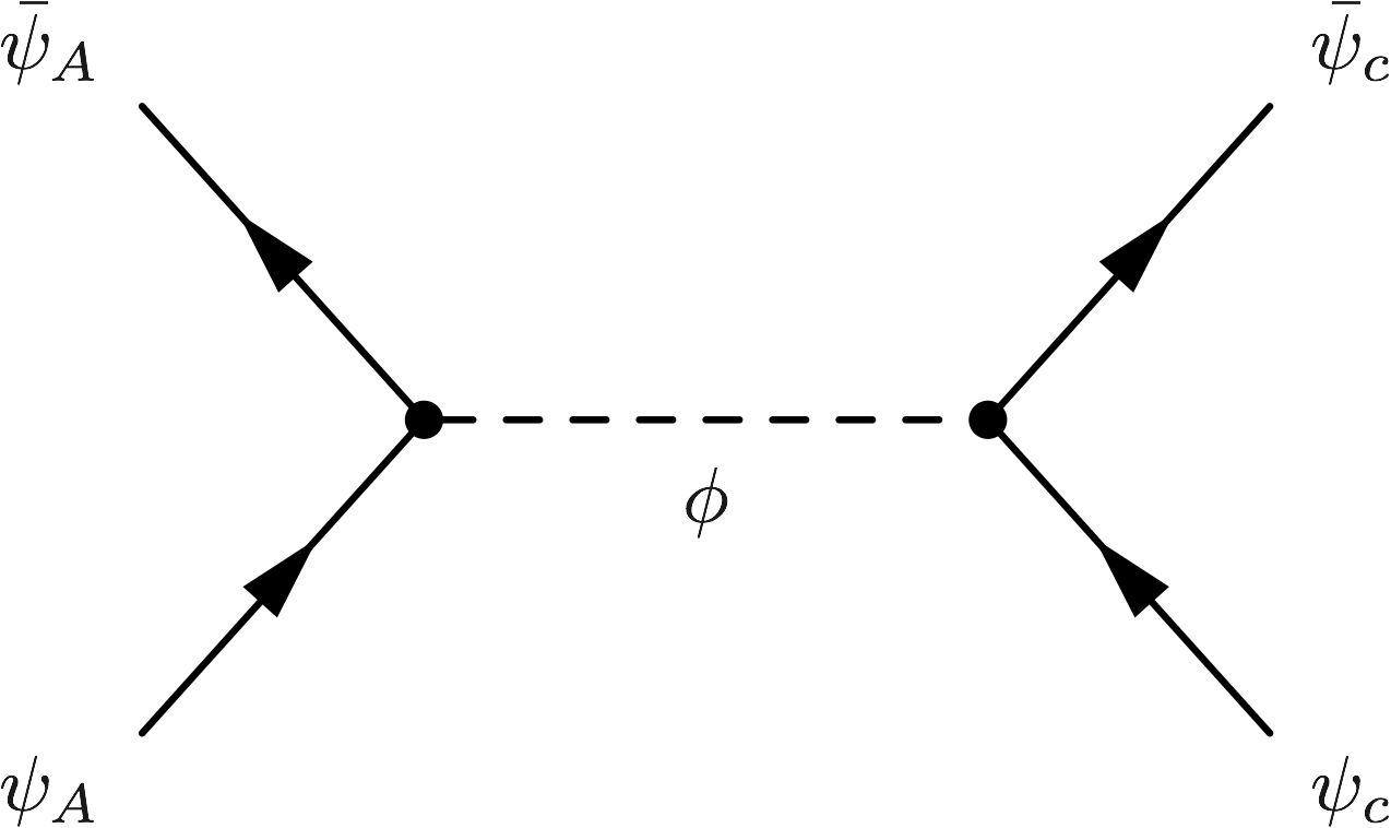
Figure 1: A Yukawa potential is generated at tree level from the exchange of $\phi$.

1.2 Model with quadratic DM couplings

The same analysis for the DDM and EP bounds on a linear $\phi$ theory can be extended to quadratic interactions. We focus on a CP invariant quadratic $\phi^{2}$ theory, given by the following effective Lagrangian

$$\mathcal{L}_{\text{quad-int}}\!=\frac{\phi^{2}}{2}\left[\frac{d^{(2)}_{e}}{4M_{\text{Pl}}^{2}}F^{\mu\nu}F_{\mu\nu}-\frac{d^{(2)}_{g}\beta_{g}}{2M_{\rm Pl}^{2}\,\,g}G^{b\mu\nu}G^{b}_{\mu\nu}-\frac{d^{(2)}_{m_{i}}}{M_{\rm Pl}^{2}\,}m_{i}\psi_{i}\psi^{c}_{i}+\text{h.c.}\right],$$ (1.8)

where the $d^{(2)}_{i}$ are the dimensionless quadratic couplings.

Since $\phi$ acquires a time-dependent vacuum expectation value (VEV) as in Eq. (1.1), oscillations of fundamental constants will be generated similarly to the linear theory, but with a background value of $\left\langle\phi^{2}\right\rangle$ instead of $\left\langle\phi\right\rangle$. For example, the variation of a constant $Y_{i}$ can be written as,

$$\frac{\delta Y_{i}(t)}{Y_{i}}\simeq\;\Delta\kappa_{i}\frac{d^{(2)}_{i}}{2M_{\text{Pl}}^{2}}\left\langle\phi^{2}\right\rangle\simeq\Delta\kappa_{i}\frac{d^{(2)}_{i}}{M_{\text{Pl}}^{2}}\frac{\rho_{\text{DM}}}{m_{\phi}^{2}}\cos^{2}\left(m_{\phi}t+\delta\right)$$ (1.9)

One should note that since the temporal modulation of the fundamental constant should follow a $\cos^{2}\left(m_{\phi}t\right)$ behavior, a bound on $\left(\delta Y_{i}(t)/Y_{i}\right)$ at an angular frequency $\nu$ should be interpreted as a bound on the couplings of a DM candidate with a mass of $m_{\phi}=\frac{\hbar\nu}{2c^{2}}$. Moreover, since the time-averaged value of $\left\langle\cos^{2}\left(m_{\phi}t\right)\right\rangle=\frac{1}{2}$, there is an additive constant contribution to the fundamental coupling constants. In this work, we are interested in timescales on which DM density variations, and decoherence effects can be neglected. For a discussion related to the slow variation of the DM amplitude see e.g. Stadnik:2014tta ; Stadnik:2015kia (cosmological evolution) and Masia-Roig:2022net (velocity dispersion decoherence).

The EP bounds on the quadratic interactions are of different nature than the EP bounds on the linear theory. In the quadratic theory, there is no Yukawa potential generated at tree level. However the time and space dependent background value of $\left\langle\phi^{2}\right\rangle$, in the presence of a massive central object, results with an effective long range force. In Appendix C, we analyze the obtained background value of $\left\langle\phi^{2}\right\rangle$ and its affect on the acceleration of a test body, and compare it to the 1-loop quantum corrections of $\phi^{2}$. We find that in the regime of our interest of ULDM, the quantum corrections are negligible compared to the classical ones. See Banks:2020gpu for a discussion of the Yukawa force for generalised potentials. Below, we take a closer look at the profile of $\phi$ and its implications to EP and DDM bounds.

1.2.1 The profile of quadratically coupled DM, boundary condition dependence

The dynamics related to quadratic coupling have a strong dependence on the boundary conditions. In our analysis, we assume that far away from the Earth, $\phi$ takes its galactic DM background, following Hees:2018fpg . This assumption is somewhat idealistic since the Earth is moving in the solar system, which consists of the moon, other planets, and the Sun, in addition to our solar system moving within the galactic medium, all perturbing the value of the scalar. In that way, it might not be entirely realistic to set the value of $\phi$ to its vacuum solution, assuming it is only be affected by the Earth, as this may depend on other variables such as the relaxation time and the dynamical history of the formation of the scalar background Bar:2018acw ; Budnik:2020nwz ; Balkin:2021zfd ; Bar:2021kti .

Alternatively, one can assume other boundary conditions and consider the phenomenology of a transient scalar background Dailey_2020 . In fact the affect of gravitational focusing of ultralight DM in the solar system was recently analyzed in PhysRevD.105.063032 where it was shown that it leads to some changes to the distribution of the ultralight DM, distribution that would have a preferred direction due to the velocity of the Sun in the DM galactic halo. Finally, the self interaction of the DM in the presence of a central gravitational potential, is expected to modify the ULDM distribution, but requires a dedicated focused study beyond the scope of this paper, as reported in haloformation . For the sake of concreteness and despite the fact that the analysis might be incomplete, we shall follow the treatment of Hees:2018fpg , assuming trivial DM background at infinity as in Eq. (1.1).

These boundary conditions lead to two important implications; the first is that the field is mediating long-distance forces despite being massive, and the second is a screening behavior near the surface of a massive source. Given the boundary conditions discussed above, the solution to the Equation of Motion (EOM) extracted from Eq. (1.8) near a massive central object yields the following analytical solution to $\phi$

$$\phi\left(t,x\right)=\phi_{0}\cos\left(m_{\phi}t+\delta\right)\left[1-s_{C}^{\left(2\right)}[d_{i}^{(2)}]\,\frac{GM_{C}}{r}\right]\,,$$ (1.10)

where $\phi_{0}\equiv\sqrt{2\rho_{\rm DM}}/m_{\phi}$ is the background amplitude of $\phi$ at infinity, $s^{(2)}_{C}[d^{(2)}_{i}]$ is some function of the quadratic couplings (explained in Appendix A), $G$ is Newton’s gravitational constant and $M_{C}$ the mass the central body, see subsection B for additional details.

In this Section, we follow two limits: the weakly coupled limit and the strongly coupled limit. In those limits, the solution takes the following form

$$\phi\left(t,x\right)=\phi_{0}\cos\left(m_{\phi}t+\delta\right)\begin{cases}\left[1-\frac{R_{C}}{r}\left(1-\sqrt{\frac{d_{i}^{\rm crit}}{d^{(2)}_{i}}}\right)\right]\,{\rm for}\,\,\,d^{(2)}_{i}\gg d_{i}^{\rm crit}\\ \left[1-\frac{R_{C}}{r}\frac{d^{(2)}_{i}}{3\,d_{i}^{\rm crit}}\right]\,\,{\rm for}\,\,\,d^{(2)}_{i}\ll d_{i}^{\rm crit}\,,\end{cases}$$ (1.11)

where the critical value of the coupling is defined as $d_{i}^{\rm crit}=R_{C}/(3Q^{C}_{i}GM_{C})$, where $R_{C}$ is the radius of the central body. Therefore, for a given DM mass $m_{\phi}$, there exists a critical value of the quadratic coupling $d^{(2)}$, at which the background value of $\left\langle\phi^{2}\right\rangle$ is screened, and thus the sensitivity to quadratically coupled ULDM is suppressed. This can be seen by taking the limit $r\rightarrow R_{C}$ in Eq.(1.11), when the DDM sensitivity becomes

$$\eta^{\rm DDM}\left(\omega\right) =\mathcal{F}_{\omega}\left(\left(\frac{\delta Y_{i}}{Y_{i}}(t)\right)^{\text{DDM-quad}}_{d^{(2)}_{i}\gg d_{i}^{\rm crit},r\simeq R_{c}}\right)\simeq\;\frac{\Delta\kappa d^{(2)}_{i}}{2M_{\text{Pl}}^{2}}\mathcal{F}_{\omega}\left(\left\langle\phi^{2}\right\rangle\right)$$

$$\simeq\Delta\kappa\frac{\phi_{0}^{2}}{M_{\text{Pl}}^{2}}\,\left[d_{i}^{\rm crit}+\frac{\Delta r}{R_{C}}d_{i}^{(2)}\sqrt{\frac{d_{i}^{\rm crit}}{d^{(2)}_{i}}}+\left(\frac{\Delta r}{R_{C}}\right)^{2}d_{i}^{(2)}\right]\times\mathcal{F}_{\omega}\left(\cos^{2}\left(m_{\phi}t+\delta\right)\right)$$

$$\simeq\Delta\kappa\frac{\phi_{0}^{2}}{M_{\text{Pl}}^{2}}\,d_{i}^{\rm crit}\times\mathcal{F}_{\omega}\left(\cos^{2}\left(m_{\phi}t+\delta\right)\right)\,,$$ (1.12)

where $\frac{\Delta r}{r}\equiv\frac{r-R_{c}}{r}\ll 1$.

Finally, we comment on the negative coupling scenario (when the sign of the DM quadratic coupling is opposite relative to the mass term). In this case, the loss of control over the system is related to the fact that if inside the Earth the mass is too negative, it would overcome the pressure gradient from the kinetic term of the order of $1/R_{C}$. Thus, it would lead to tachyonic instabilities (where within the Earth, the mass squared of the field is negative) and to a runaway behavior of the field into large-amplitudes inside and outside Budnik:2020nwz ; Balkin:2021zfd ; Hook:2019pbh .

1.3 Summary of EP and DDM sensitivities

We end this introduction by summarizing the sensitivities again, $\eta^{\rm DDM}$ and $\eta^{\rm EP}$, and provide their full description as a function of the DM scalar field background. The complete derivation of these sensitivities can be found in Appendix A. For the linear couplings DM model, we found:

$$\eta^{\rm EP}_{\text{linear}}=2\frac{|\vec{a}_{A,C}-\vec{a}_{B,C}|}{|\vec{a}_{A,C}+\vec{a}_{B,C}|}\simeq\frac{|\Delta Q_{i}d^{(1)}_{i}\vec{\nabla}V_{C}\left(\phi\right)|}{M_{\text{Pl}}GM_{C}/r^{2}}\simeq\frac{\Delta Q_{i}d^{(1)}_{i}}{M_{\text{Pl}}GM_{C}/r^{2}}\left[\nabla\phi\left(x,t\right)+\vec{v}\dot{\phi}\left(x,t\right)\right]\,,$$ (1.13)

$$\eta^{\rm DDM}_{\text{linear}}\left(\omega\right)=\mathcal{F}_{\omega}\left(\frac{\delta Y(t)}{Y}\right)\simeq\frac{\Delta\kappa_{i}^{A}d^{(1)}_{i}}{M_{\text{Pl}}}\mathcal{F}_{\omega}\left(\left\langle\phi\left(x,t\right)\right\rangle\right)\,.$$ (1.14)

In both equation (1.13) and (1.14), the letters A and B represent two different test bodies, while C denotes the central heavy object such as the Earth. $d^{(1)}_{i}$ is the linear DM coupling to the $i^{\text{th}}$ SM field. For the quadratic DM model, we find

$$\eta^{\rm EP}_{\text{quad}}=2\frac{|\vec{a}_{A,C}-\vec{a}_{B,C}|}{|\vec{a}_{A,C}+\vec{a}_{B,C}|}\simeq\frac{\Delta Q_{i}d^{(2)}_{i}}{M^{2}_{\text{Pl}}GM_{C}/r^{2}}\phi\left(x,t\right)\left[\nabla\phi\left(x,t\right)+\vec{v}\dot{\phi}\left(x,t\right)\right]\,,$$ (1.15)

$$\eta^{\rm DDM}_{\text{quad}}\left(\omega\right)=\mathcal{F}_{\omega}\left(\frac{\delta Y(t)}{Y}\right)\simeq\frac{{\Delta\kappa_{i}^{A}d^{(2)}_{i}}}{2M_{\text{Pl}}^{2}}\mathcal{F}_{\omega}\left(\left\langle\phi^{2}\left(x,t\right)\right\rangle\right)\,.$$ (1.16)

Finally, we present the approximate sensitivities given the specific DM background solution of Eq. (1.10) with its special boundary conditions. For the linear DM model, we get

$$\eta^{\rm EP}_{\text{linear}}=2\frac{|\vec{a}_{A,C}-\vec{a}_{B,C}|}{|\vec{a}_{A,C}+\vec{a}_{B,C}|}\simeq Q^{C}_{j}d^{(1)}_{j}\Delta Q_{i}d^{(1)}_{i}e^{-m_{\phi}r}\,,$$ (1.17)

$$\eta^{\rm DDM}_{\text{linear}}\left(m_{\phi}\right)=\frac{|\delta Y(t)|}{Y}\simeq\frac{\Delta\kappa_{i}^{A}d^{(1)}_{i}}{M_{\text{Pl}}}\phi_{0}\,.$$ (1.18)

Lastly, the results for the quadratic DM model are

$$\eta^{\rm EP}_{\text{quad}}=2\frac{|\vec{a}_{A,C}-\vec{a}_{B,C}|}{|\vec{a}_{A,C}+\vec{a}_{B,C}|}\simeq\Delta Q_{i}d^{(2)}_{i}s_{C}^{\left(2\right)}[d^{(2)}_{i}]\left(\Delta Q\right)_{j}^{AB}d^{(2)}_{j}\frac{\phi_{0}^{2}}{2M^{2}_{\text{Pl}}}\left[1-s_{C}^{\left(2\right)}\frac{GM_{C}}{r}\right]\,,$$ (1.19)

$$\eta^{\rm DDM}_{\text{quad}}\left(2m_{\phi}\right)=\frac{|\delta Y(t)|}{Y}\simeq\frac{{\Delta\kappa_{i}^{A}d^{(2)}_{i}}}{4M_{\text{Pl}}^{2}}\phi_{0}^{2}\,\left[1-s_{C}^{\left(2\right)}\frac{GM_{C}}{r}\right]^{2}\,.$$ (1.20)

2 Updated Bounds from EP and DDM searches

In this Section we present the bounds on the DM models both from EP and DDM searches. We also discuss the interplay between the EP and DDM searches for the linear and the quadratically coupled DM with the SM. We also discuss two proposed ways to alleviate the EP test constraints in details and present the reach of DDM searches in those scenarios.

2.1 Summary of current and future bounds

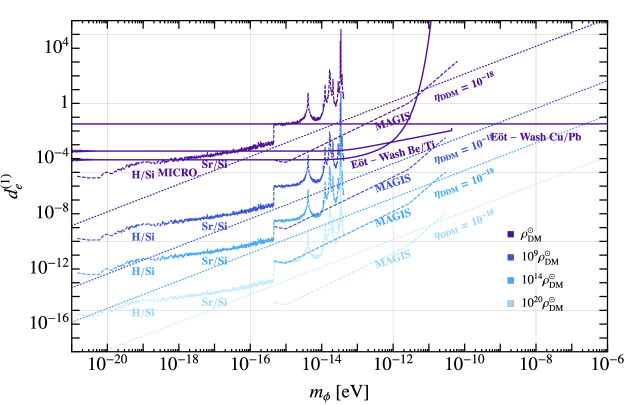
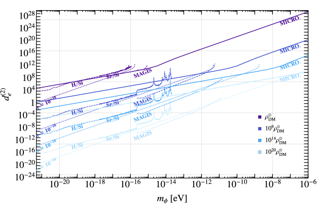
Figure 3: Top: the bounds on $d_{e}^{(1)}$ from the linear DM photon couplings. Bottom: the bounds on $d_{e}^{(2)}$ from the quadratic DM photon couplings. Note the bounds in Kennedy:2020bac were modified for the assumption of a stochastic DM background.

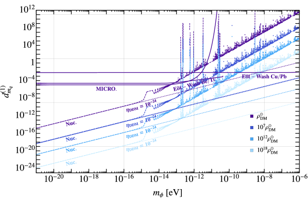
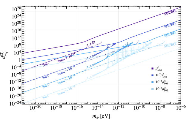
Figure 4: Top: the bounds on $d_{m_{q}}^{(1)}$ from the linear DM light quarks couplings. Bottom: the bounds on $d_{m_{q}}^{(2)}$ from the quadratic DM light quarks couplings.

The known bounds on scalar, pseudo-scalar and quadratic DM interactions with the SM are summarized in Tables 1-3 for various ULDM masses. In addition, we also present current and future-projected bounds on the linear scalar couplings $d^{(1)}_{i}$ and on the quadratic couplings $d^{(2)}_{i}$ as a function of the DM mass for various local DM densities, up to $10^{5}$ the DM density at the solar position $\rho_{\text{DM}}^{\odot}$ Salucci:2010qr , as motivated by Pitjev_2013 ; Tsai:2022jnv ; haloformation . The bounds for the electron couplings, $d_{m_{e}}$, are shown in Figure 2, the bounds for the photon couplings, $d_{e}$, are shown in Figure 3, the bounds for the quark couplings, $d_{m_{q}}$, are shown in Figure 4, and the bounds for the gluon couplings, $d_{g}$, are shown in Figure 5. For all linear couplings, the EP test bounds are derived from the terrestrial Eöt-Wash Be/Ti Schlamminger:2007ht and Eöt-Wash Cu/Pb PhysRevD.61.022001 measurements, as well as from the MICROSCOPE data PhysRevLett.129.121102 taken on a satellite orbiting the Earth at an approximate altitude of 700 km. For the quadratic couplings, we present only the bounds from MICROSCOPE, which are expected to be the strongest Hees:2018fpg . The current DDM bounds for $d_{m_{e}}$ are given from the H/Si clock-cavity comparison measurements presented in Kennedy:2020bac . For $d_{e}$, the current DDM bounds are given both from H/Si and Sr/Si clock-cavity comparisons Kennedy:2020bac , where for masses larger than $\sim 10^{-16}$ eV an additional measurement with using dynamical decoupling was applied to improve the sensitivity at high frequencies Aharony:2019iad . For both $d_{m_{e}}$ and $d_{e}$, we also show a line representing a DDM sensitivity of $\eta_{\rm DDM}=10^{-18}$ at all masses, as well as the expected bound from the future DDM MAGIS-100 experiment Abe_2021 . A DDM experiment involving hyperfine transitions Kennedy:2020bac ; Hees:2016gop and/or vibrational levels of a molecule Oswald:2021vtc can be used to constraint DM couplings to nucleus i.e. $d_{m_{q}}$ and $d_{g}$. However, here we present the expected bounds from a nuclear clock with a sensitivity of $\eta_{\rm DDM}=10^{-24}$, using a Ramsey sequence with the parameters given in Banerjee:2020kww . The astrophysical constraints mentioned in Tables 1-3, are coming from various stellar cooling processes as mentioned in the given references.

$$\boxed{m_{\phi}=10^{-8}\,\,{\rm eV}}$$

operator	current bound	type of experiment
$\frac{d^{(1)}_{e}}{4\,M_{\text{Pl}}}\phi\,F^{\mu\nu}F_{\mu\nu}$	$d^{(1)}_{e}\lesssim 10^{-2}$ PhysRevD.61.022001	EP test: Eöt-Wash Cu/Pb
$\frac{\tilde{d}^{(1)}_{e}}{M_{\text{Pl}}}\phi\,F^{\mu\nu}\tilde{F}_{\mu\nu}$	$\tilde{d}^{(1)}_{e}\lesssim 2\times 10^{8}$ Anastassopoulos:2017ftl	axion/ALP searches: CAST
$\frac{\left|d^{(1)}_{m_{e}}\right|}{M_{\text{Pl}}}\phi\,m_{e}\psi_{e}\psi_{e}^{c}$	$\left|d^{(1)}_{m_{e}}\right|\lesssim 1$ PhysRevD.61.022001	EP test: Eöt-Wash Cu/Pb
$i\frac{\left|\tilde{d}^{(1)}_{m_{e}}\right|}{M_{\text{Pl}}}\phi\,m_{e}\psi_{e}\psi_{e}^{c}$	$\left|\tilde{d}^{(1)}_{m_{e}}\right|\lesssim 8\times 10^{8}$ Capozzi:2020cbu	Astrophysics
$\frac{d^{(1)}_{g}\beta(g)}{2M_{\text{Pl}}\,g}\phi\,G^{\mu\nu}G_{\mu\nu}$	$d^{(1)}_{g}\lesssim 10^{-3}$ PhysRevD.61.022001	EP test: Eöt-Wash Cu/Pb
$\frac{\tilde{d}^{(1)}_{g}}{M_{\text{Pl}}}\phi\,G^{\mu\nu}\tilde{G}_{\mu\nu}$	$\tilde{d}^{(1)}_{g}\lesssim 10^{8}$ Raffelt:2006cw ; Buschmann:2021juv	Astrophysics
$\frac{\left|d^{(1)}_{m_{N}}\right|}{M_{\text{Pl}}}\phi\,m_{N}\psi_{N}\psi_{N}^{c}$	$\left|d^{(1)}_{m_{N}}\right|\lesssim 6\times 10^{-3}$ Schlamminger:2007ht	EP test: Eöt-wash 2008
$i\frac{\left|\tilde{d}^{(1)}_{m_{N}}\right|}{M_{\text{Pl}}}\phi\,m_{N}\psi_{N}\psi_{N}^{c}$	$\left|\tilde{d}^{(1)}_{m_{N}}\right|\lesssim 3\times 10^{8}$ Beznogov:2018fda	Astrophysics
$\frac{d^{(2)}_{e}}{8M^{2}_{\text{Pl}}}\phi^{2}\,F^{\mu\nu}F_{\mu\nu}$	$d^{(2)}_{e}\lesssim 10^{25}$ PhysRevLett.129.121102	EP test: MICROSCOPE
$\frac{\left|d^{(2)}_{m_{e}}\right|}{2M^{2}_{\text{Pl}}}\phi^{2}\,m_{e}\psi_{e}\psi_{e}^{c}$	$\left|d^{(2)}_{m_{e}}\right|\lesssim 10^{27}$ PhysRevLett.129.121102	EP test: MICROSCOPE
$\frac{d^{(2)}_{g}\beta_{g}}{4M_{\rm Pl}^{2}\,\,g}\phi^{2}\,G^{\mu\nu}G_{\mu\nu}$	$d^{(2)}_{g}\lesssim 10^{25}$ PhysRevLett.129.121102	EP test: MICROSCOPE
$\frac{\left|d^{(2)}_{m_{N}}\right|}{2M^{2}_{\text{Pl}}}\phi^{2}\,m_{N}\psi_{N}\psi_{N}^{c}$	$\left|d^{(2)}_{m_{N}}\right|\lesssim 10^{25}$ PhysRevLett.129.121102	EP test: MICROSCOPE

Table 1: Strongest existing bounds on various DM couplings for a mass of the order of $m_{\phi}=10^{-8}\,\,{\rm eV}$.

$$\boxed{m_{\phi}=10^{-15}\,\,{\rm eV}}$$

operator	current bound	type of experiment
$\frac{d^{(1)}_{e}}{4\,M_{\text{Pl}}}\phi\,F^{\mu\nu}F_{\mu\nu}$	$d^{(1)}_{e}\lesssim 10^{-4}$ PhysRevLett.129.121102	EP test: MICROSCOPE
$\frac{\tilde{d}^{(1)}_{e}}{M_{\text{Pl}}}\phi\,F^{\mu\nu}\tilde{F}_{\mu\nu}$	$\tilde{d}^{(1)}_{e}\lesssim 2\times 10^{6}$ Reynolds:2019uqt	Astrophysics
$\frac{\left|d^{(1)}_{m_{e}}\right|}{M_{\text{Pl}}}\phi\,m_{e}\psi_{e}\psi_{e}^{c}$	$\left|d^{(1)}_{m_{e}}\right|\lesssim 10^{-3}$ PhysRevLett.129.121102	EP test: MICROSCOPE
$i\frac{\left|\tilde{d}^{(1)}_{m_{e}}\right|}{M_{\text{Pl}}}\phi\,m_{e}\psi_{e}\psi_{e}^{c}$	$\left|\tilde{d}^{(1)}_{m_{e}}\right|\lesssim 8\times 10^{8}$ Capozzi:2020cbu	Astrophysics
$\frac{d^{(1)}_{g}\beta(g)}{2M_{\text{Pl}}\,g}\phi\,G^{\mu\nu}G_{\mu\nu}$	$d^{(1)}_{g}\lesssim 6\times 10^{-6}$ PhysRevLett.129.121102	EP test: MICROSCOPE
$\frac{\tilde{d}^{(1)}_{g}}{M_{\text{Pl}}}\phi\,G^{\mu\nu}\tilde{G}_{\mu\nu}$	$\tilde{d}^{(1)}_{g}\lesssim 10^{8}$ Raffelt:2006cw ; Buschmann:2021juv	SN1987A, NS
$\frac{\left|d^{(1)}_{m_{N}}\right|}{M_{\text{Pl}}}\phi\,m_{N}\psi_{N}\psi_{N}^{c}$	$\left|d^{(1)}_{m_{N}}\right|\lesssim 6\times 10^{-6}$ PhysRevLett.129.121102	EP test: MICROSCOPE
$i\frac{\left|\tilde{d}^{(1)}_{m_{N}}\right|}{M_{\text{Pl}}}\phi\,m_{N}\psi_{N}\psi_{N}^{c}$	$\left|\tilde{d}^{(1)}_{m_{N}}\right|\lesssim 3\times 10^{8}$ Beznogov:2018fda	Astrophysics
$\frac{d^{(2)}_{e}}{8M^{2}_{\text{Pl}}}\phi^{2}\,F^{\mu\nu}F_{\mu\nu}$	$d^{(2)}_{e}\lesssim 10^{11}$ PhysRevLett.129.121102	EP test: MICROSCOPE
$\frac{\left|d^{(2)}_{m_{e}}\right|}{2M^{2}_{\text{Pl}}}\phi^{2}\,m_{e}\psi_{e}\psi_{e}^{c}$	$\left|d^{(2)}_{m_{e}}\right|\lesssim 10^{12}\,$ PhysRevLett.129.121102	EP test: MICROSCOPE
$\frac{d^{(2)}_{g}\beta_{g}}{4M_{\rm Pl}^{2}\,\,g}\phi^{2}\,G^{\mu\nu}G_{\mu\nu}$	$d^{(2)}_{g}\lesssim 10^{11}$ PhysRevLett.129.121102	EP test: MICROSCOPE.
$\frac{\left|d^{(2)}_{m_{N}}\right|}{2M^{2}_{\text{Pl}}}\phi^{2}\,m_{N}\psi_{N}\psi_{N}^{c}$	$\left|d^{(2)}_{m_{N}}\right|\lesssim 10^{11}$ PhysRevLett.129.121102	EP test: MICROSCOPE

Table 2: Strongest existing bounds on various DM couplings for a mass of the order of $m_{\phi}=10^{-15}\,\,{\rm eV}$.

$$\boxed{m_{\phi}=10^{-18}\,\,{\rm eV}}$$

operator	current bound	type of experiment
$\frac{d^{(1)}_{e}}{4\,M_{\text{Pl}}}\phi\,F^{\mu\nu}F_{\mu\nu}$	$d^{(1)}_{e}\lesssim 10^{-4}\,$ Kennedy:2020bac	DDM oscillations
$\frac{\tilde{d}^{(1)}_{e}}{M_{\text{Pl}}}\phi\,F^{\mu\nu}\tilde{F}_{\mu\nu}$	$\tilde{d}^{(1)}_{e}\lesssim 2\times 10^{6}$ Reynolds:2019uqt	Astrophysics
$\frac{\left|d^{(1)}_{m_{e}}\right|}{M_{\text{Pl}}}\phi\,m_{e}\psi_{e}\psi_{e}^{c}$	$\left|d^{(1)}_{m_{e}}\right|\lesssim 2\times 10^{-3}$ Kennedy:2020bac	DDM Oscillations
$i\frac{\left|\tilde{d}^{(1)}_{m_{e}}\right|}{M_{\text{Pl}}}\phi\,m_{e}\psi_{e}\psi_{e}^{c}$	$\left|\tilde{d}^{(1)}_{m_{e}}\right|\lesssim 7\times 10^{8}$ Capozzi:2020cbu	Astrophysics
$\frac{d^{(1)}_{g}\beta(g)}{2M_{\text{Pl}}\,g}\phi\,G^{\mu\nu}G_{\mu\nu}$	$d^{(1)}_{g}\lesssim 6\times 10^{-6}$ PhysRevLett.129.121102	EP test: MICROSCOPE
$\frac{\tilde{d}^{(1)}_{g}}{M_{\text{Pl}}}\phi\,G^{\mu\nu}\tilde{G}_{\mu\nu}$	$\tilde{d}^{(1)}_{g}\lesssim 4$ Abel:2017rtm	Oscillating neutron EDM
$\frac{\left|d^{(1)}_{m_{N}}\right|}{M_{\text{Pl}}}\phi\,m_{N}\psi_{N}\psi_{N}^{c}$	$\left|d^{(1)}_{m_{N}}\right|\lesssim 2\times 10^{-6}$ PhysRevLett.129.121102	EP test: MICROSCOPE
$i\frac{\left|\tilde{d}^{(1)}_{m_{N}}\right|}{M_{\text{Pl}}}\phi\,m_{N}\psi_{N}\psi_{N}^{c}$	$\left|\tilde{d}^{(1)}_{m_{N}}\right|\lesssim 4$ Abel:2017rtm	Oscillating neutron EDM
$\frac{d^{(2)}_{e}}{8M^{2}_{\text{Pl}}}\phi^{2}\,F^{\mu\nu}F_{\mu\nu}$	$d^{(2)}_{e}\lesssim 10^{6}$ Kennedy:2020bac	DDM oscillations
$\frac{\left|d^{(2)}_{m_{e}}\right|}{2M^{2}_{\text{Pl}}}\phi^{2}\,m_{e}\psi_{e}\psi_{e}^{c}$	$\left|d^{(2)}_{m_{e}}\right|\lesssim 10^{6}\,$ Kennedy:2020bac	DDM oscillations
$\frac{d^{(2)}_{g}\beta_{g}}{4M_{\rm Pl}^{2}\,\,g}\phi^{2}\,G^{\mu\nu}G_{\mu\nu}$	$d^{(2)}_{g}\lesssim 10^{7}$ PhysRevLett.129.121102	EP test: MICROSCOPE.
$\frac{\left|d^{(2)}_{m_{N}}\right|}{2M^{2}_{\text{Pl}}}\phi^{2}\,m_{N}\psi_{N}\psi_{N}^{c}$	$\left|d^{(2)}_{m_{N}}\right|\lesssim 10^{7}$ PhysRevLett.129.121102	EP test: MICROSCOPE

Table 3: Strongest existing bounds on various DM couplings for a mass of the order of $m_{\phi}=10^{-18}\,\,{\rm eV}$.

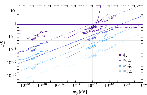
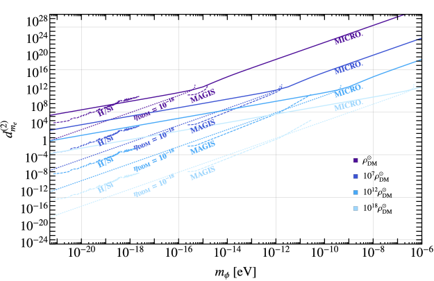
Figure 2: Top: the bounds on $d_{m_{e}}^{(1)}$ from the linear DM electrons couplings. Bottom: the bounds on $d_{m_{e}}^{(2)}$ from the quadratic DM electron couplings.

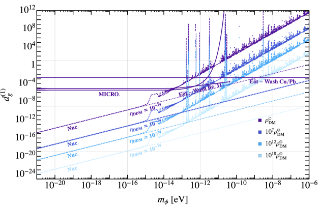
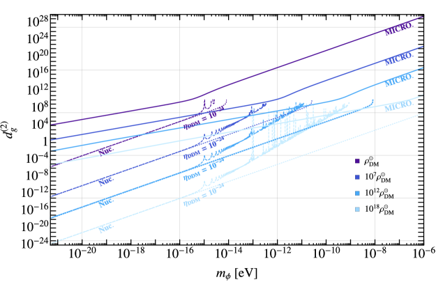
Figure 5: Top: the bounds on $d_{g}^{(1)}$ from the linear DM gluon couplings. Bottom: the bounds on $d_{g}^{(2)}$ from the quadratic DM gluon couplings.

2.2 Complementarity of EP tests and DDM searches

We can compare the bounds on the DM couplings coming from DDM experiments to the ones coming from EP tests, both for linear and quadratic interactions. We begin by summarizing the scaling of the DDM and EP bounds, both in the linear and quadratic theories, as presented in Table 4.

	linear theory: $\frac{d_{i}^{(1)}}{M_{\text{Pl}}}\phi\,\mathcal{O}^{i}_{\rm SM}$	quadratic theory: $\frac{d_{i}^{(2)}}{2M_{\text{Pl}}^{2}}\phi^{2}\,\mathcal{O}^{i}_{\rm SM}$
DDM bounds: $\left(\frac{\delta Y_{i}}{Y}(t)\right)<\eta_{\text{DDM}}$	$\frac{d_{i}^{(1)}}{M_{\text{Pl}}}\frac{\sqrt{2\rho_{\text{DM}}}}{m_{\phi}}$	$\frac{d_{i}^{(2)}}{2M_{\text{Pl}}^{2}}\frac{\rho_{\text{DM}}}{m_{\phi}^{2}}$
EP bounds: $\left(\frac{\delta a_{\text{test}}}{a}\right)<\eta_{\text{EP}}$	$\left(d_{i}^{(1)}d_{j}^{(1)}\right)\Delta Q_{i}^{\text{test}}Q_{j}^{\text{Earth}}$	$\frac{1}{M_{\text{Pl}}^{2}}\left(d_{i}^{(2)}d_{j}^{(2)}\right)\Delta Q_{i}^{\text{test}}Q_{j}^{\text{Earth}}\,\frac{\rho_{\text{DM}}}{m_{\phi}^{2}}$
Ratio: $\frac{\left(d\right)_{\text{DDM}}}{\left(d\right)_{\text{EP}}}$	$\frac{M_{\text{Pl}}m_{\phi}\sqrt{\Delta Q_{i}^{\text{test}}Q_{i}^{\text{Earth}}}}{\sqrt{2\rho_{\text{DM}}}}\,\frac{\eta_{\text{DDM}}}{\sqrt{\eta_{\text{EP}}}}$	$\frac{2M_{\text{Pl}}m_{\phi}\sqrt{\Delta Q_{i}^{\text{test}}Q_{i}^{\text{Earth}}}}{\sqrt{\rho_{\text{DM}}}}\,\frac{\eta_{\text{DDM}}}{\sqrt{\eta_{\text{EP}}}}$

Table 4: Theoretical estimation of the bounds on the linear and quadratic couplings between the light scalar DM and the SM light fields. $\eta_{\text{DDM}}$ and $\eta_{\text{EP}}$ are defined as the sensitivity of the DDM and EP experiments, respectively. $Y$ is a fundamental constant $Y\in(\alpha,\alpha_{s},m_{f})$ and $\mathcal{O}_{\rm SM}$ is the appropriate SM operator $\mathcal{O}_{\rm SM}\in\left(\frac{1}{4}F^{\mu\nu}F_{\mu\nu}\,,\frac{\beta(g)}{2g}G_{a}^{\mu\nu}G^{a}_{\mu\nu}\,,m_{i}\psi_{i}\psi_{i}^{c}\right)$. The spatial dependence of the bounds is disregarded (equivalent to taking the $m_{\phi}\ll 1/R_{C}$ limit for the linear case and the $d^{(2)}_{i}\ll d_{i}^{\rm crit}$ limit for the quadratic case).

As one can easily read from Table 4, the ratio of the bounded couplings from different types of experiments, i.e., the ratio: $\left(d\right)_{\text{DDM}}/\left(d\right)_{\text{EP}}$ has the same parametric dependence in both the linear and the quadratic theory, as long as the spatial dependence of the bounds may be neglected (namely, away from the Yukawa decoupling of the linear bounds and in the sub-critical region for the quadratic bounds). Therefore, under these conditions, if one type of experiment dominates the bounds on the linear interaction in some region of the parameter space, we expect it to also dominate the bounds on the quadratic couplings and vice versa. As is further shown in the table, in agreement with the plots above, DDM experiments tend to be more powerful at lower masses. Their corresponding constraints improve linearly with the experimental sensitivity, whereas EP tests are expected to take over at higher masses while scaling only with the square root of the experimental sensitivity.

While one of these searches usually dominates the bounds for specific masses, we would like to argue that EP-tests and the DDM searches are complementary to each other and provide independent information. Below we point out two engaging scenarios in which the naive ratio between EP and DDM bounds is violated, demonstrating their complementary.

2.2.1 Enhanced DM Density

The current EP bounds for the quadratic theory and the DDM bounds for both the linear and the quadratic couplings strongly depend on the local DM density. These bounds become more stringent if the on-Earth DM density is enhanced compared to the DM density at the solar position $\rho_{\text{DM}}^{\odot}$ Salucci:2010qr , as would be the case if a compact boson star consisting of $\phi$ is formed in the early universe, and is gravitationally bounded to the Sun or the Earth Banerjee:2019epw ; Banerjee:2019xuy ; haloformation . Importantly, note that DDM searches are more sensitive to the local DM density than EP tests, and thus the ratio of their corresponding bounds $d_{i}^{\text{DDM}}/d_{i}^{\text{EP}}$ would vary with the density. The ratios $d_{i}^{\text{DDM}}/d_{i}^{\text{EP}}$, are presented as a function of the DM on-Earth density enhancement $\rho_{\text{DM}}/\rho_{\text{DM}}^{\odot}$ for a few different benchmark DM masses in Figs. 6-7. Although a density enhancement factor much larger than $10^{5}$ is currently not motivated by theoretical or experimental considerations Pitjev_2013 ; Tsai:2022jnv ; haloformation , higher densities are included for completeness. For $\left(d_{m_{e}}\right)^{\text{DDM}}/\left(d_{m_{e}}\right)^{\text{EP}}$ and $\left(d_{e}\right)^{\text{DDM}}/\left(d_{e}\right)^{\text{EP}}$ in Fig 6, the atomic/molecular clock sensitivity is taken to be $\eta_{\text{DDM}}=10^{-18}$ for all values of $m_{\phi}$. For $\left(d_{m_{q}}\right)^{\text{DDM}}/\left(d_{m_{q}}\right)^{\text{EP}}$ and $\left(d_{g}\right)^{\text{DDM}}/\left(d_{g}\right)^{\text{EP}}$ in Fig 7, the nuclear clock sensitivity is taken to be $\eta_{\text{DDM}}=10^{-24}$ for all values of $m_{\phi}$. The EP sensitivity is taken from current experiments and depends on the mass of the DM.

As expected, an enhanced DM density would make the ratio between the DDM bounds and the EP bounds smaller. In particular, for the electron coupling and for the photon coupling, the hierarchy between the two searches may be flipped for masses greater than $\sim 10^{-15}\,{\rm eV}$. In addition, for the quadratic interactions, the DM density enhancement could also effectively shift the onset of the critical behavior to higher masses, making DDM searches sensitive to the quadratic couplings at these masses, as opposed to the $\rho_{\text{DM}}=\rho_{\text{DM}}^{\odot}$ case. Therefore, when considering the possibility of a larger DM density, the DDM and EP searches may have competing sensitivities, making them complimentary.

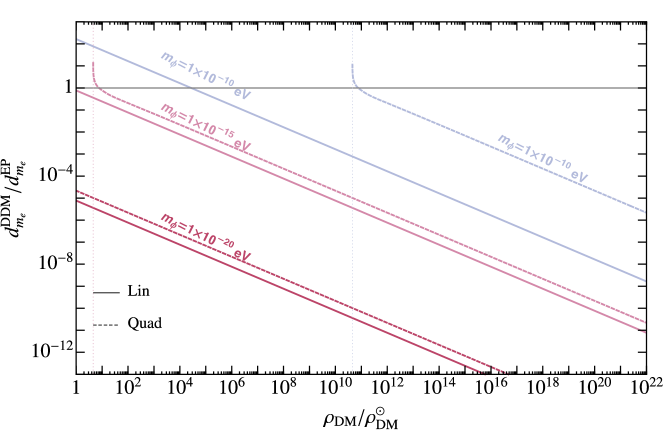
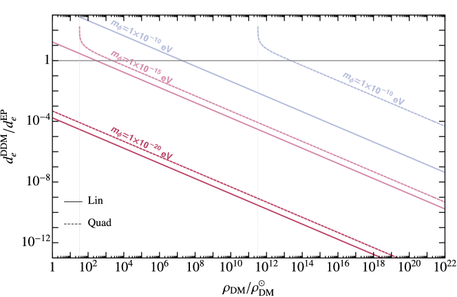
Figure 6: Ratio between DDM bounds and EP bounds on the DM-SM electron coupling $d_{m_{e}}$ (top) and photon coupling $d_{e}$ (bottom) as a function of the on-Earth DM density enhancement, relative to the DM density at the solar position $\rho_{\text{DM}}^{\odot}$. Solid – ratio for the linear coupling $d^{(1)}$, dashed – ratio for the quadratic coupling $d^{(2)}$. The vertical lines mark the minimal density enhancement required to probe sub-critical quadratic couplings by DDM tests. The DDM sensitivity is taken to be $\eta_{\text{DDM}}=10^{-18}$ for all DM masses $m_{\phi}$. The EP bound is taken as from existing EP-tests results.

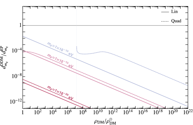
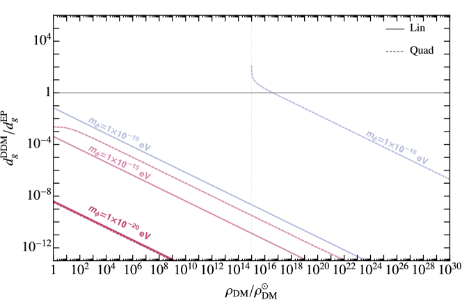
Figure 7: Ratio between DDM bounds and EP bounds on the DM-SM quark coupling $d_{m_{q}}$ (top) and the gluon coupling $d_{g}$ (bottom) as a function of the on-Earth DM density enhancement, relative to the DM density at the solar position $\rho_{\text{DM}}^{\odot}$. Solid – ratio for the linear coupling $d^{(1)}$, dashed – ratio for the quadratic coupling $d^{(2)}$. The vertical lines mark the minimal density enhancement required to probe sub-critical quadratic couplings by DDM tests. The DDM sensitivity is taken to be $\eta_{\text{DDM}}=10^{-24}$ for all DM masses $m_{\phi}$. The EP bound is taken as from existing EP-tests results.

2.2.2 Non-generic couplings

Let us discuss the bounds from the EP test experiments, which are generically stronger than the constraints arising from the DDM searches for individual coupling in the region $10^{-18}\,{\rm eV}\lesssim m_{\phi}\lesssim\mathcal{O}(\,{\rm eV})$ Kennedy:2020bac ; Hees:2018fpg . As discussed, the EP tests compare the dilatonic charges of two test bodies. To calculate the “dilatonic charge" of an atom a with $Z$($N$) being the number of protons (neutrons), one can write the mass of an atom $m^{\bf a}$ as, $m^{\bf a}(Z,N)=m^{\bf a}_{\rm nuc}(Z,N)+Zm_{e}\,,$ where, $m^{\bf a}_{\rm nuc}$ is the mass of the nucleus of a. Furthermore, the nucleus mass contribution can be decomposed in terms of the proton ($m_{p}$) and the neutron ($m_{n}$) masses, and the binding energy of the strong ($E_{3}$) and electromagnetic ($E_{1}$) interaction as, $m^{\bf a}_{\rm nuc}(Z,N)=Zm_{p}+Nm_{n}+E_{3}+E_{1}\,.$ Note that $E_{1}$ is dominated by the EM force within the nucleus, and thus we will ignore the electrons’ effect on it Damour:2010rp . For a generic atom a, the dilatonic charges, $\vec{Q}^{\bf a}$, can be written as Damour:2010rp ,

$$\!\!\vec{Q}^{\mathbf{a}}\!\approx\!F^{\mathbf{a}}\!\!\left(\!3\!\times\!10^{-4}-4\,r_{I}+8\,r_{Z}\,,\,3\!\times\!10^{-4}-3\,r_{I}\,,\,0.9\,,0.09-\frac{0.04}{A^{1/3}}-2\times 10^{6}r_{I}^{2}-r_{Z},0.002\,r_{I}\!\right)\!.$$

In what follows we use the following notation for a vector $\vec{X}\equiv X_{e,m_{e},g,\hat{m},\delta m}$ , with $\hat{m}\equiv(m_{d}+m_{u})/2$ , $\delta m\equiv(m_{d}-m_{u}),$ $10^{4}\,r_{I;Z}\equiv 1-2Z/A;Z(Z-1)/A^{4/3}\,,$ and $F^{\mathbf{a}}=931\,A^{\mathbf{a}}/(m^{\mathbf{a}}/{\rm MeV})$ with $A^{\mathbf{a}}$ being the atomic number of the atom a. The MICROSCOPE experiment Touboul:2017grn ; PhysRevLett.129.121102 ; Berge:2017ovy , which provides the strongest EP bounds for masses below $10^{-12}\,$eV, is sensitive to the difference between the dilatonic charges of Platinum/Rhodium alloy (90/10) and Titanium/Aluminum/Vanadium (90/6/4) which is given by

$$(\stackrel{{\scriptstyle\longrightarrow}}{{\Delta Q\ }})^{\rm Mic}\simeq 10^{-3}(-1.94\,,\,0.03\,,\,0.8\,,\,-2.61\,,\,-0.19)\,.$$

$(\stackrel{{\scriptstyle\longrightarrow}}{{\Delta Q\ \!}})$ for other experiments looking for EP violation are discussed in Oswald:2021vtc . We find that these sensitivities map to directions in the five-dimensional ULDM coupling space that are very different from that of DDM searches, denoted by $(\stackrel{{\scriptstyle\longrightarrow}}{{\Delta\kappa\ }})^{\rm DDM}$, which usually have $\mathcal{O}(1)$ sensitives for variations in $\alpha$ and $m_{e}$ (e.g. Safronova:2019lex ; Antypas:2019yvv ; Antypas:2020rtg and refs. therein). Examining the four best EP bounds, Cu-Pb PhysRevD.61.022001 , Be-Ti Schlamminger:2007ht , and Be-Al Wagner:2012ui along with the previously mentioned MICROSCOPE experiment, in the five-dimensional vector space of coupling, we can construct a combination that would be orthogonal to all of them, approximately given by,

$$\hat{Q}^{\perp}\sim\big{(}0.01\,,\,0.99\,,\,0.01\,,\,-0.01\,,\,0.13\,\big{)}\,.$$ (2.1)

It implies that models of light scalar DM with coupling direction defined according to $\hat{Q}^{\perp}\cdot\vec{d}$ would not be subject to these four leading EP bounds.

Here for simplicity, we consider an ULDM quadratically coupled to the SM and assume two scenarios:

1. A model where only $d^{(2)}_{m_{e}}\neq 0$,

2. A model defined by a vector of sensitivities, $\hat{Q}^{\perp}\cdot\,\vec{d}^{(2)}$, that is orthogonal to the sensitivities of the four leading EP test experiments.

We present the bounds on these two models in Figure 8 by the solid and the dashed lines, respectively. For the second model, we have projected the bounds on $d^{(2)}_{m_{e}}$ as $\hat{Q}^{\perp}$ has a relatively significant overlap with the direction corresponding to $m_{e}$ (the second entry of it, which is the largest). Also for simplicity we have considered a DDM search experiment, which only depends on $m_{e}$ and thus the sensitivity vector can be written as $(\stackrel{{\scriptstyle\longrightarrow}}{{\Delta\kappa\ }})^{\rm DDM}=(\,0,1,0,0,0)\,$. Note that, due to the large overlap of $\hat{Q}^{\perp}$ with the $m_{e}$ direction, the specific choice of $(\stackrel{{\scriptstyle\longrightarrow}}{{\Delta\kappa\ }})^{\rm DDM}$ has a negligible effect on the final conclusion. In our case, $\hat{Q}^{\perp}\cdot(\stackrel{{\scriptstyle\longrightarrow}}{{\Delta\kappa\ }})^{\rm DDM}\simeq 0.99$, which is approximately the sensitivity coefficients corresponding to $m_{e}$. In addition, the sensitivity of both the EP tests and the DDM searches depend on the geometry of the source body as discussed in Eqs. (1.19) and (1.20) respectively. We also assume a homogeneous spherically symmetric Earth as the source body, which is made of $32\%$ Iron and $68\%$ silicon oxide. With the above assumption, we get the dilatonic charge of the source body as

$$Q^{\rm source}\simeq 10^{-3}\,(\,1.87\,,\,0.27\,,\,1000.19\,,\,80.51\,,\,0.04\,)\,.$$ (2.2)

As mentioned below Eq. (B.6), the critical value of a coupling is inversely proportional to the corresponding dilatonic charge of the source. In Figure 8, we see that $d_{m_{e}}^{\rm crit}$ (shown by the solid yellow line) is $35$ times larger than the critical value of the second model which is defined by a vector of sensitivities, $\hat{Q}^{\perp}\cdot\,\vec{d}^{(2)}$ (shown by the dashed yellow line) as $Q^{\rm source}\cdot\hat{Q}^{\perp}=9.49\times 10^{-3}$, whereas $Q^{\rm source}_{m_{e}}=0.27\times 10^{-3}$. Unlike the first model, where only $d_{m_{e}}^{(2)}\neq 0$, the second model is not constrained by the four leading EP experiments. In the $\hat{Q}^{\perp}$ direction, the strongest EP bound is coming from the Be-Cu test Su:1994gu (the fifth best one), which is more than five orders of magnitude weaker than the MICROSCOPE PhysRevLett.129.121102 experiment, which provides the most stringent bound for any model with only one non-zero coupling Hees:2018fpg . The turquoise and the pink lines in Figure 8 depict the strongest bounds from the EP tests on the first and the second models, respectively. The black lines depict the bounds from DDM searches located on the surface of the Earth, whereas the red and the blue lines represent bounds from DDM searches located 400 km (average altitude of the International Space Station) and 5000 km above the surface of the Earth (see FOCOS clock proposal), respectively. See Section 3.2 for more details. We have assumed the sensitivity of the DDM searches to be $\eta_{\rm DDM}=10^{-18}$. Note that, below criticality, even the terrestrial DDM searches provide stronger bounds than the EP tests for both the scenarios discussed here. These bounds are $\mathcal{O}(10^{5})$ stronger than that of the EP test in the lower mass region. As explained before, for a given sensitivity, the reach of the space-based DDM searches is better than the Earth-based ones due to the screening effect of theories with quadratic couplings. Above $m_{\phi}\gtrsim 2\times 10^{-16}\,{\rm eV}$, the bound from the MICROSCOPE experiment is slightly stronger than that of the space-based DDM searches for the first scenario, where only $d_{m_{e}}^{(2)}\neq 0$. However, for the second scenario, due to the considerable overlap of $\hat{Q}^{\perp}$ with the $m_{e}$ direction, the reach of the DDM searches is not reduced, unlike the EP tests. This allows the space-based DDM searches to provide the strongest bound even for the higher masses and above the critical value of the coupling. Around $m_{\phi}\sim 10^{-13}\,{\rm eV}$, the bounds from DDM searches are $\mathcal{O}(10^{9})$ stronger than the best EP bound (coming from the Be-Cu test shown by the dashed magenta line in Figure 8).

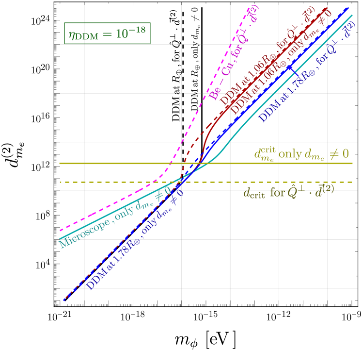
Figure 8: Exclusion plot for $d^{(2)}_{m_{e}}$; the solid lines assume a model where only $d^{(2)}_{m_{e}}\neq 0$. The dashed lines depict the bounds for a model defined by a vector of sensitivities, $\hat{Q}^{\perp}\cdot\,\vec{d}^{(2)}$, that is orthogonal to the sensitivities of four leading EP test experiments projected onto $d^{(2)}_{m_{e}}$. The black lines depict the bounds from DDM searches located on the surface of the Earth, whereas the red and the blue lines represent bounds from DDM searches located at 400 km and 5000 km above the surface of the Earth, respectively. We have assumed the sensitivity of the DDM searches is $\eta_{\rm DDM}=10^{-18}$. The magenta line depicts the strongest bound from the EP tests (which is coming from MICROSCOPE experiment PhysRevLett.129.121102 ) for only $d^{(2)}_{m_{e}}\neq 0$ models. The pink line represents the strongest EP bound for a model defined by a vector of sensitivities $\hat{Q}^{\perp}\cdot\,\vec{d}^{(2)}$(which is coming from Be-Cu test Su:1994gu ). The yellow lines represent the critical value of the couplings.

Let us consider a case where the five-dimensional coupling is universal, thus does not violate EP. As discussed in Oswald:2021vtc , if a scalar-field coupling to the SM is defined according to $\vec{Q}_{\rm dil}\cdot\vec{d}^{(i)}$ where $i=1,2$ with $\vec{Q}_{\rm dil}\simeq(-0.01,1,1,1,0)\,,$ then it will not be subjected to the EP tests bounds. However, it will still give rise to deviations from the inverse square law and, thus, will be constrained by fifth-force search experiments. To simplify our discussion, we will consider the case of a linearly coupled scalar to the SM; however, our main result also applies to a quadratically coupled theory.

To briefly see how the EP non-violation works, we know that gravity couples to the Ricci scalar $R$, and using Einstein’s equation, one can write $R\propto T^{\mu}_{\mu}$ where $T^{\mu}_{\mu}$ is the trace of the energy-momentum tensor. Thus, if a scalar-field coupling to the SM is proportional to $T^{\mu}_{\mu}$, it will not generate any EP violation. This is an idealistic limit and is realized only in pure dilaton models, where the dilaton $(\phi)$ couplings are precisely given by

$$\mathcal{L}\supset\frac{\phi}{f_{\rm dil}}T^{\mu}_{\mu}\,,$$ (2.3)

where $f_{\rm dil}$ is the conformal invariance breaking scale Dymarsky:2013pqa . As discussed before and in Damour:2010rp ; Hees:2018fpg , above interaction would induce a Yukawa interaction between two bodies. The interaction strength can be written as

$$\alpha=\frac{1}{\sqrt{4\pi G_{\rm N}}}\frac{\partial\ln m(\phi)}{\partial\phi}\propto\frac{1}{f_{\rm dil}}\,.$$ (2.4)

This shows that the dilaton coupling is universal, and the conformal invariance breaking scale determines the coupling strength. The differential acceleration between two test bodies is proportional to the difference between their Yukawa interaction strength, as shown in Eq. (A), and it vanishes due to the universality of the dilaton coupling. Thus, a pure dilaton does not generate EP violation. However, it is easy to see using Eq. (2.4) that in the presence of a source with mass $m^{\rm s}$, the acceleration of a test body can be written as

$$\vec{a}_{\rm A}=-\hat{r}\frac{G_{\rm N}\,m^{\rm S}}{r^{2}}\left[1+\frac{2M_{\rm Pl}^{2}}{f_{\rm dil}^{2}}\left(1+m_{\rm dil}\,r\right)e^{-m_{\rm dil}\,r}\right],$$ (2.5)

where $M_{\rm Pl}^{2}=1/(8\pi G_{N})$ and $m_{\rm dil}$ is the mass of the dilaton. The above equation shows that the presence of a dilaton causes deviation from $1/r^{2}$ force and thus can be constrained by various experiments that test for deviations from Newtonian gravity (fifth-force searches) (see Fischbach:1996eq and Refs. therein). We are also assuming that the dilaton would acquire a small mass from a sector other than the SM Coradeschi:2013gda in order to be a viable DM candidate Arvanitaki:2014faa .

So far, we have argued a scalar that interacts with the SM as given in Eq. (2.3) would not violate EP but would give rise to deviations from Newtonian gravity. Now to get the direction in the five-dimensional coupling space, we need to write the expression for $T^{\mu}_{\mu}$. Assuming that the SM is valid up to the scale $f_{\rm dil}$, $T^{\mu}_{\mu}$ can be written as

$$T^{\mu}_{\mu}=\frac{\beta(g)}{2g}G^{2}+\frac{\beta(g_{2})}{2g_{2}}W^{2}+\frac{\beta(y)}{2y}B^{2}+(1-\gamma)\sum_{\psi}m_{\psi}\bar{\psi}\psi\,,$$ (2.6)

where $g$, $g_{2}$ are the coupling strength of $SU(3)$ and $SU(2)$ gauge groups, respectively, $y$ represents the hypercharge corresponding to $U(1)_{y}$, and $G$, $W$ and $B$ are the corresponding gauge fields respectively. Also, $\psi$ denotes the SM fermions with mass $m_{\psi}$. For simplicity, in the above formula, we assume that the conformal breaking scale $f_{\rm dil}$ is far below the Landau pole of $U(1)_{y}$ and above the electro-weak (EW) scale. As $T^{\mu}_{\mu}$ is invariant under the evolution of the Renormalization Group (RG) equation (manifested in the above equation), the dilaton always couples through anomaly matching to the same quantity at any scale $\mu$. For our purpose, we consider our theory at $\mu=1\,{\rm GeV}$ and $T^{\mu}_{\mu}$ can be expressed as,

$$T^{\mu}_{\mu}=\frac{\beta(g_{s})}{2g_{s}}G^{2}+\frac{\beta(e)}{2e}F^{2}+\sum_{\psi}m_{\psi}\bar{\psi}\psi\,.$$ (2.7)

In the above equation, we have redefined the fermion masses in terms of their pole masses. Combining this with Eq. (2.3) and along with our convention of defining a vector in the five-dimensional coupling space, we can write the dilaton coupling vector, $\vec{Q}_{\rm dil}$ as

$$\vec{Q}_{\rm dil}=(-\frac{2\beta(e)}{e},1,1,1,0)\,,$$ (2.8)

where $e$ is the electric charge and $\beta(e)=e^{3}/(12\pi^{2})$. As below $m_{e}\sim\,{\rm MeV}$, the theory essentially becomes free, we find $2\beta(e)/e\sim e^{2}/(6\pi^{2})\times 10\sim 0.015$ as $\log(\rm GeV/\rm MeV)\sim 10$. Thus, we get $\vec{Q}_{\rm dil}=(-0.01,1,1,1,0)\,.$ Thus, we have argued that a scalar field (the dilaton), whose coupling is defined according to $\vec{Q}_{\rm dil}\cdot\vec{d}^{(1)}$, will not generate an EP-violating acceleration, as the direction is indistinguishable from that of gravity. In Fig. 9 we show the bounds from various fifth-force searches projected on the $d^{(1)}_{m_{e}}$ and $d^{(1)}_{g}$ directions on a pure dilaton model by the blue solid line. For comparison, we also show the bounds from various EP tests on a model which only couples to either $m_{e}$ or gluon field strength linearly i.e. $\mathcal{L}\supset d^{(1)}_{m_{e}}\phi\,m_{e}\bar{e}e/M_{\rm Pl}$ or $\mathcal{L}\supset d^{(1)}_{g}\beta(g)\,\phi\,G^{2}/(2g\,M_{\rm Pl})$ by the turquoise line. Various constraints on these models are shown in details in Fig. 2 and Fig. 5 respectively.

We, finally, note that if the dilaton couplings are not perfectly aligned with that obtained from the trace of the energy-momentum tensor, it will generate EP-violating acceleration as discussed in Taylor:1988nw ; Kaplan:2000hh .

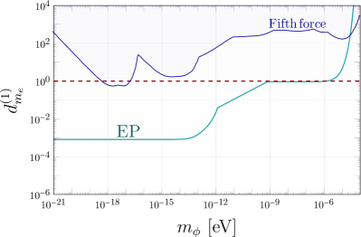
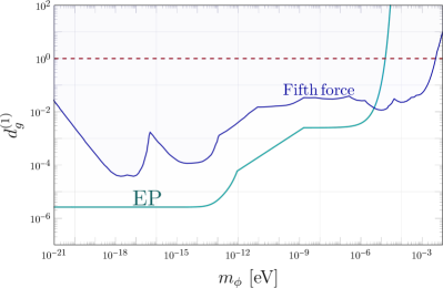
Figure 9: Bounds from various experiments which are looking for EP-violation and/or deviation from Newtonian gravity (fifth force searches) on $d^{(1)}_{m_{e}}$ (left) and $d^{(1)}_{g}$ (right). The turquoise lines show the strongest constraints from various EP violation searches PhysRevLett.129.121102 ; Wagner:2012ui ; Schlamminger:2007ht ; PhysRevD.61.022001 assuming a model where only $d^{(1)}_{i}\neq 0$ where $i=m_{e},g$. The blue lines depict the strongest bound coming from various fifth force experiments (see Fischbach:1996eq ; Lee:2020zjt ; Tan:2020vpf and Refs. therein). The red dashed lines indicate $d^{(1)}_{i}=1$.

3 Quadratic Interactions and Screening

In the previous section, we observed that the bounds on the quadratic couplings are weaker than the bounds on the linear couplings. One reason is the cutoff-suppression, attenuating the effects of the quadratic coupling by a factor of $\phi/\Lambda_{\rm UV}$ compared to those of the linear coupling, where $\Lambda_{\rm UV}$ is the UV scale that characterizes the EFT. This happens as a quadratic couplings represents a higher-dimensional effective operator than the linear one.

The other reason is the fact that the quadratic coupling might be screened at the surface of a central body as discussed in Section 1.2.1, as well as in Appendix A, and previously in Hees:2018fpg . Below we discuss two important scenarios that alter the effects of the screening behavior. The first is a theoretical one - a model in which both linear and quadratic couplings are present simultaneously, and the second is an experimental one - positioning DDM experiments in space.

3.1 Screening and criticality in a model with both linear and quadratic couplings

Let us discuss the sensitivity of EP tests and DDM searches in the presence of both linear and quadratic couplings between the ULDM and the SM. While the interplay of linear and quadratic interactions has been previously discussed in the context of non-DM models Olive:2007aj , the DM boundary condition plays a crucial role in setting the field’s profile, and thus leads to qualitatively and quantitatively different results. As we will show here, a theory with linear and quadratic couplings has more severely constrained linear and quadratic couplings than a theory with only one of the couplings turned on. Also, in the presence of both the couplings, there is a small region of the parameter space where the DDM bounds are stronger than those of the EP tests.

The Lagrangian of that model can be written as

$$\mathcal{L}=\mathcal{L}_{\text{lin-int}}+\mathcal{L}_{\text{ quad-int}}\,,$$ (3.1)

where $\mathcal{L}_{\text{lin-int}}$ and $\mathcal{L}_{\text{ quad-int}}$ are defined in Eq. (1.2) and Eq. (1.8) respectively. As we are interested in calculating the sensitivities of DDM searches and EP tests, we would like to solve for the profile of $\phi$. As discussed above, we assume a homogeneous boundary condition at large distances for $\phi$ i.e.

$$\phi(r\to\infty,t)=\phi_{0}\cos(m_{\phi}t+\delta)\,,$$ (3.2)

with $\phi_{0}=\sqrt{2\rho_{\rm DM}}/m_{\phi}$. The EOM of this combined model is

$$\left(\frac{\partial^{2}}{\partial t^{2}}-\nabla\cdot\nabla+\tilde{m}_{\phi}^{2}\left(r\right)\right)\phi=J_{\text{source}}\left(r\right)\,,$$ (3.3)

where we define

$$\tilde{m}_{\phi}^{2}\left(r\right)\equiv m_{\phi}^{2}+\frac{Q_{i}^{C}d_{i}^{(2)}}{M_{\text{Pl}}^{2}}\rho_{C}\left(r\right)\,\,{\rm and}\,\,\,\,J_{\text{source}}\left(r\right)\equiv-\frac{Q^{C}_{i}d_{i}^{\left(1\right)}}{M_{\text{Pl}}}\rho_{C}\left(r\right).$$ (3.4)

Notice that the linear coupling, $d_{i}^{(1)}$, provides a source term for the EOM whereas the quadratic coupling $d_{i}^{(2)}$ modifies the mass term of $\phi$. As discussed in Hees:2018fpg , in the presence of a source body $C$, the SM fields can be replaced by the density of the source body $\rho_{C}\left(r\right)$ with corresponding dilatonic charge $Q_{i}^{C}$, where $i$ runs over the SM species coupled to the ULDM. If we model the source body $C$ as a uniform density sphere of radius $R_{C}$ and mass $M_{C}$, then one can write

$$\rho_{C}\left(r\right)=\begin{cases}\frac{3M_{C}}{4\pi R_{C}^{3}}&r\leq R_{C}\\ 0&r>R_{C}\,.\end{cases}$$ (3.5)

See the discussion around Eq. (B.1) for more details. The solution of the EOM given in Eq. (3.3) with the boundary condition of Eq. (3.2) can be written as

$$\phi\left(r,t\right)= \begin{cases}\phi_{0}\,{\rm cs}\,\frac{\text{sinhc}\left(\frac{r}{R_{C}}\sqrt{d_{i}^{(2)}/d_{i}^{\rm crit}}\right)}{\cosh\left[\sqrt{d_{i}^{(2)}/d_{i}^{\rm crit}}\right]}-M_{C}\frac{r^{2}}{R_{C}^{3}}\frac{Q^{C}_{j}d_{j}^{\left(1\right)}}{M_{\text{Pl}}}I\left(\tilde{m}_{\phi}r\right)\frac{e^{-\tilde{m}_{\phi}r}}{4\pi}&r<R_{C}\\ \phi_{0}\,{\rm cs}\,\left(1-s_{C}[d_{i}^{(2)}]\frac{GM_{C}}{r}\right)-M_{C}\frac{Q^{C}_{j}d_{j}^{\left(1\right)}}{M_{\text{Pl}}}I\left(m_{\phi}R_{c}\right)\frac{e^{-m_{\phi}r}}{4\pi r}&r\geq R_{C}\,,\end{cases}$$ (3.6)

where we define ${\rm cs}=\cos\left(m_{\phi}t+\delta\right)$ and the functions $I(x)$ and $s_{C}[d_{i}^{(2)}]$ are given by

$$I(x)=3\,\dfrac{x\cosh x-\sinh x}{x^{3}}\,,\,\,s^{(2)}_{C}[d^{(2)}_{i}]=Q^{C}_{i}d^{(2)}_{i}J_{+}\left(\sqrt{d^{(2)}_{i}/d_{i}^{\rm crit}}\right)\,.$$ (3.7)

In addition, $d_{i}^{\rm crit}=R_{C}/(3Q^{C}_{i}GM_{C})$ as defined before, and the function $J_{+}(x)$ is defined as $J_{+}(x)=3(x-\tanh x)/x^{3}$ Hees:2018fpg . $G$ and $M_{\rm Pl}$ can be used interchangeably with $4\pi G=1/M_{\rm Pl}^{2}\,$. Using the solution of the EOM for $r\geq R_{C}$, and assuming the signal will be time averaged, we get the sensitivity of the EP tests as

$$\!\!\!\!\!\!\!\!\!\!\!\!\!\!\!\!\!\!\!\!\!\!\!\!\!\!\!\!\!\!\!\!\!\!\!\!\eta^{\text{EP}}(r) = 2\frac{|\vec{a}_{A,C}-\vec{a}_{B,C}|}{|\vec{a}_{A,C}+\vec{a}_{B,C}|}\simeq\frac{\left(\Delta Q\right)_{i}^{AB}}{GM_{C}/r^{2}}\left(\frac{d^{(1)}_{i}}{M_{\text{Pl}}}+\frac{d^{(2)}_{i}}{M^{2}_{\text{Pl}}}\phi\right)|\vec{\nabla}\phi|$$ (3.8)

$$\simeq \,\left(\Delta Q\right)_{i}^{AB}\Bigg{(}s_{C}^{\left(2\right)}[d_{j}^{(2)}]d^{(2)}_{i}\frac{\phi_{0}^{2}}{2M^{2}_{\text{Pl}}}\left[1-s_{C}^{\left(2\right)}[d_{j}^{(2)}]\frac{GM_{C}}{r}\right]$$

$$+Q^{C}_{j}d_{j}^{(1)}d^{(1)}_{i}\,I(m_{\phi}R_{C})\,(1+m_{\phi}r)\,e^{-m_{\phi}r}$$

$$-\left(Q^{C}_{j}d_{j}^{(1)}\right)^{2}d^{(2)}_{i}\frac{G\,M_{C}}{r}I(m_{\phi}R_{C})^{2}\,(1+m_{\phi}r)\,e^{-2m_{\phi}r}\Bigg{)}\,,$$

and the sensitivity of DDM searches as

$$\eta^{\text{DDM}}_{\omega}(r)= \;\frac{|\delta Y(t)|}{Y}\approx\frac{\Delta\kappa_{i}d_{i}^{(2)}}{2M_{\text{Pl}}^{2}}\,\times\phi_{0}^{2}\left(1-s_{C}[d_{j}^{(2)}]\frac{GM_{C}}{r}\right)^{2}\mathcal{F}_{\omega}\left({\rm cs}^{2}\right)$$

$$-\; \frac{\Delta\kappa_{i}d_{i}^{(2)}}{M_{\text{Pl}}^{2}}\frac{M_{C}Q^{C}_{j}d_{j}^{\left(1\right)}}{M_{\text{Pl}}}I\left(m_{\phi}R_{c}\right)\frac{e^{-m_{\phi}r}}{4\pi r}\times\phi_{0}\,\left[1-s_{C}[d_{k}^{(2)}]\frac{GM_{C}}{r}\right]\mathcal{F}_{\omega}\left(\rm cs\right)$$

$$+\; \frac{\Delta\kappa_{i}d_{i}^{(1)}}{M_{\text{Pl}}}\,\times\phi_{0}\,\left(1-s^{(2)}_{C}[d_{j}^{(2)}]\frac{GM_{C}}{r}\right)\mathcal{F}_{\omega}\left({\rm cs}\right)\,.$$ (3.9)

We want to describe the screening effect in this model. As most of the DDM searches are terrestrial, in this section we consider them to be performed very close to the surface of the source body, i.e., at $r\simeq R_{C}$. In Section 3.2 we discuss the space based DDM searches where $r\gtrsim R_{C}$.

As discussed before, in a model where the DM interacts only quadratically with the SM, if the coupling is larger than the critical value, the DDM sensitivity is screened, and the dependence on the quadratic couplings is suppressed. However, in a model with both linear and quadratic couplings, due to the mixed $d^{(2)}d^{(1)}$ term, there is no such criticality for the DDM searches.

To see how it works, let us start with the case when $d^{(2)}_{i}\gg d_{i}^{\rm crit}$. In this limit $s^{(2)}_{C}[d^{(2)}_{i}]$ can be written as Eq. (B.6) and we get,

$$1-s^{(2)}_{C}[d_{i}^{(2)}]\frac{GM_{C}}{r}=\sqrt{\frac{d_{i}^{\rm crit}}{d^{(2)}_{i}}}+\mathcal{O}\left(\frac{\Delta r}{R_{C}}\right)\,,$$ (3.10)

and Eq. (3.1) becomes

$$\left.\eta^{\text{DDM}}(\omega)\right|_{\left(d^{(2)}_{i}\gg d_{i}^{\rm crit},\>r\simeq R_{c}\right)} \approx\frac{\Delta\kappa_{i}}{M_{\text{Pl}}^{2}}\phi_{0}^{2}\,\,d_{i}^{\rm crit}\times\mathcal{F}_{\omega}\left({\rm cs}^{2}\right)$$

$$-\frac{\Delta\kappa_{i}}{M_{\text{Pl}}}\phi_{0}\,\left[\frac{Q^{C}_{j}}{3Q^{C}_{i}}d_{j}^{(1)}\sqrt{\frac{d_{i}^{(2)}}{d_{i}^{\rm crit}}}\right]I\left(m_{\phi}R_{c}\right)e^{-m_{\phi}R_{c}}\times\mathcal{F}_{\omega}\left({\rm cs}\right)$$

$$+\frac{\Delta\kappa_{j}}{M_{\text{Pl}}}\phi_{0}\,\left[d_{j}^{(1)}\sqrt{\frac{d_{i}^{\rm crit}}{d_{i}^{(2)}}}\right]\times\mathcal{F}_{\omega}\left({\rm cs}\right)+\mathcal{O}\left(\frac{\Delta r}{R_{C}}\right)\,.$$ (3.11)

As expected, the above equation shows that if we have only quadratic couplings, i.e., $d_{i}^{(1)}=0$, then DDM searches become insensitive to the quadratic couplings, as the sensitivity does not depend on $d^{(2)}_{i}$ in the supercritical limit. However when $d_{i}^{(1)}\neq 0$, it is sensitive to $\sqrt{d_{i}^{(2)}}$. We can further simplify the above expression for $m_{\phi}\ll 1/R_{C}$ as

$$\!\!\left.\eta^{\text{DDM}}\left(\omega\right)\right|_{\left(d^{(2)}_{i}\gg d_{i}^{\rm crit},\>r\simeq R_{c}\ll 1/m_{\phi}\right)}\approx-\frac{\Delta\kappa_{j}}{3M_{\text{Pl}}}\phi_{0}\,d_{j}^{(1)}\sqrt{\frac{d_{i}^{(2)}}{d_{i}^{\rm crit}}}\times\mathcal{F}_{\omega}\left({\rm cs}\right)+\mathcal{O}\left(\frac{\Delta r}{R_{C}},\frac{d_{i}^{\rm crit}}{d_{i}^{(2)}}\right)\,,$$ (3.12)

and for $m_{\phi}\gg 1/R_{C}$ as

$$\left.\eta^{\text{DDM}}\right|_{\left(d^{(2)}_{i}\gg d_{i}^{\rm crit},\>r\simeq R_{c}\gg 1/m_{\phi}\right)}\approx\frac{\Delta\kappa_{j}}{M_{\text{Pl}}}\phi_{0}\,d_{j}^{(1)}\sqrt{\frac{d_{i}^{(2)}}{d_{i}^{\rm crit}}}\left(\frac{d_{i}^{\rm crit}}{d_{i}^{(2)}}-\frac{1}{2m_{\phi}^{2}R_{C}^{2}}\right)\times\mathcal{F}_{\omega}\left({\rm cs}\right)+\mathcal{O}\left(\frac{\Delta r}{R_{C}}\right)\,,$$ (3.13)

by noting the limiting case of the function $I(x)$

$$\lim_{x\to 0}I(x)\to 1\,\,{\rm and}\,\,\lim_{x\to\infty}I(x)e^{-x}\to\frac{1}{2x^{2}}\,.$$ (3.14)

For completeness we also discuss the case of small quadratic coupling, $d^{(2)}_{i}\ll d_{i}^{\rm crit}$. In this case $s_{C}[d^{(2)}_{i}]\simeq Q^{C}_{i}d^{(2)}_{i}$ and Eq. (3.1) becomes

$$\left.\eta^{\text{DDM}}\right|_{\left(d^{(2)}_{i}\ll d_{i}^{\rm crit},\>r\simeq R_{c}\right)}\simeq\frac{\Delta\kappa_{i}d_{i}^{(2)}}{2M_{\text{Pl}}^{2}}\,\times\phi_{0}^{2}\,{\rm cs}^{2}+\frac{\Delta\kappa_{i}d_{i}^{(1)}}{M_{\text{Pl}}}\,\times\phi_{0}\,{\rm cs}+\mathcal{O}\left(\frac{d_{i}^{(2)}}{d_{i}^{\rm crit}}\right)\!,\!\!$$ (3.15)

for all masses.

In Figures. 10-11, we present the allowed parameter space of a model with both the linear and quadratic couplings for different masses of the DM. We notice that introducing a non-zero quadratic coupling changes the bounds on the linear coupling and vice-versa. This means that a theory that has both linear and quadratic couplings has a stronger constraint on each compared to a theory with only one of the couplings. Despite that, we see that in most of the parameter space of interest, the EP bounds from the linear coupling are still the dominant ones. Due to the scalar field profile in the presence of both linear and quadratic couplings, there is a small region of the parameter space where the DDM bounds are stronger than the EP bounds, as can be seen in all the figures below. This could be of potential interest to DDM searches whose accuracy has improved vastly in the last few years.

The above observation motivates us to present a few models where the linear couplings are suppressed compared to the quadratic ones. We require that these theories are natural in the sense that there is no fine-tuning in order to achieve such hierarchies between the small values of the linear coupling compared to the relatively large values of the quadratic coupling. We present two such models within the Clockwork framework in Section 5.4, and another model of within the Relaxed Relaxion framework in Section 6.2.3.

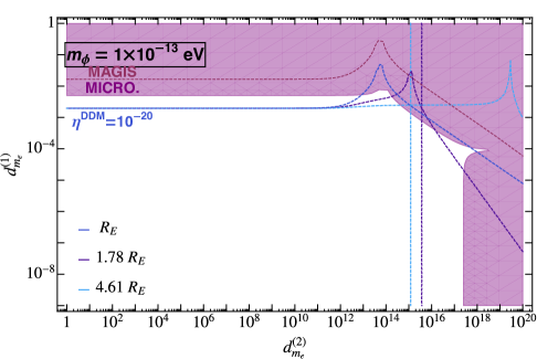
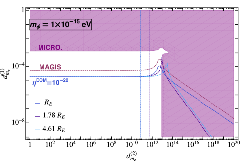
Figure 10: Allowed parameter space for the linear and quadratic electron coupling for masses of $m_{\phi}=10^{-13}\,\,{\rm eV}\,\text{{(top)}},\>10^{-15}\,\,{\rm eV}\,\text{{(bottom)}}$.

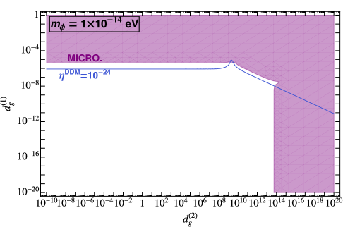
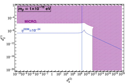
Figure 11: Allowed parameter space for the linear and quadratic gluon coupling for masses of $m_{\phi}=10^{-14}\,\,{\rm eV}\,\text{{(top)}},\>10^{-15}\,\,{\rm eV}\,\text{{(bottom)}}$.

3.2 Screening and criticality in space

Since the screening of the ULDM is most dominant at the surface of the Earth, experiments done further away are less affected by it, as can be seen by Eq. (1.11). This is the key to the dominance of the MICROSCOPE EP test, positioned at an altitude of roughly $700$ km, over the bounds on the quadratic coupling. If, however, DDM searches are also performed in geocentric orbits, they too would become sensitive to the ULDM quadratic couplings. To demonstrate this point, we show in Fig. 12 the bounds on the electron coupling and photon coupling, $d^{(2)}_{m_{e}}$ and $d^{(2)}_{e}$ respectively, as expected for DDM experiments with sensitivities of $10^{-18}$, and $10^{-20}$, located at 400 km, 5000 km, and 23000 km above the surface of the Earth. Below we survey some of the recent proposals with the potential to launch highly sensitive DDM experiments into space.

The NASA Deep Space Atomic Clock (DSAC) mission has recently demonstrated a microwave trapped ion clock based on Hg⁺ ions achieving a factor of $10$ improvement over previous space-based clocks Burt2021 . The such clock was proposed for the auto-navigation of spacecraft 2018Navigation . Cold atom microwave clock was demonstrated in space in CAC2018 . The ACES (Atomic Clock Ensemble in Space) mission ACES is planned to perform an absolute measurement of the red-shift effect between the microwave PHARAO clock on-board the International Space Station (ISS) and clocks on Earth, to improve such limit by an order of magnitude.

The progress in the development of optical clocks has been extraordinary, with three orders of magnitude improvement in uncertainty over the last 15 years LudBoyYe15 . Several optical clocks have reached uncertainty at the 10^-18 level (see, e.g., PhysRevLett.123.033201 ), with further improvements expected as there is no apparent technical limit. Portable high-precision optical clocks were also demonstrated KelBurKal19 , which is a prerequisite for space deployment. Various clock-comparisons and clock-cavity comparison experiments are sensitive to $d_{e}^{(i)}$, $d_{m_{e}}^{(i)}$, and $d_{g}^{(i)}$. The applications of the different clock types of clocks and optical cavities for ULDM searches were recently reviewed in 2022UDM .

Deployment of high-precision optical clocks in space will enable both practical and fundamental applications, including tests of general relativity FOCOS , DM searches Sun , gravitational wave detection in new wavelength ranges Kolkowitz_2016 ; Fedderke:2021kuy , relativistic geodesy Puetzfeld:2019kki , linking Earth optical clocks Gozzard:2021wkf , and others. The roadmap for cold atom technologies in space has been outlined in roadmap . In the present work, we demonstrate another window of opportunity to study ULDM with clocks in space, taking advantage of the space environments that are drastically different from that of the Earth. Being away from the Earth’s surface allows us to test the quadratic models described above. We used orbital parameters of proposal FOCOS as an example in Section 2.2.2. Ref. FOCOS describes a space mission concept that would place a state-of-the-art optical atomic clock in an eccentric orbit around Earth. The main mission goal is to test the gravitational red-shift, a classical test of general relativity, with sensitivity 30,000 times beyond current limits by comparing clocks on Earth and the spacecraft. A high stability laser link between the Earthbound and space clocks is needed to connect the relative time, range, and velocity of the orbiting spacecraft to Earthbound stations. In general relativity, the tick rate of time slows in the presence of massive bodies, and locating one or more clocks in orbits around the Earth provides a low-noise environment for tests of gravity. Sr high-precision optical atomic clock aboard an Earth-orbiting space station (OACESS) OACESS was proposed for DM searches, including static or quasi-static apparent variations of $m_{e}$ with changing height above Earth’s surface and transient changes in the apparent value of $\alpha$ due to the passage of a relativistic scalar wave from an intense burst of extraterrestrial origin. The goal of this pathfinder mission is to compare the space-based high-precision optical atomic clock (OAC) with one or more ultra-stable terrestrial OACs to search for space-time-dependent signatures of dark scalar fields that manifest as anomalies in the relative frequencies of station-based and ground-based clocks. The OACESS will serve as a pathfinder for dedicated missions (e.g., FOCOS described above FOCOS ) to establish high-precision OAC as space-time references in space. We used the orbital parameters of the International Space Station ($\sim$ 400 km above the surface of the Earth) and FOCOS mission proposal FOCOS in Fig. 8 and Fig. 12.

A version of the such proposal with a state-of-the-art cavity will enable test the quadratic models by also running a clock-cavity experiment as carried out in Kennedy:2020bac , sensitive to $d_{e}^{(2)}$ coupling. We note that a time transfer link to Earth is not required for such an experiment. The clock-comparison experiment in space involving a molecular clock will also be sensitive to $d_{m_{e}}^{(2)}$. Molecular clocks are projected to reach $10^{-18}$ uncertainties HanKuzLun21 .

In Ref. Sun , a clock-comparison satellite mission with two clocks onboard to the inner reaches of the solar system was proposed to search for a DM halo bound to the Sun and to look for the spatial variation of the fundamental constants associated with a change in the gravitation potential. Various clock combinations were considered to provide sensitivities to various couplings. This work showed that the projected sensitivity of space-based clocks for the detection of Sun-bound DM halo exceeds the reach of Earth-based clocks by orders of magnitude. This mission in its proposed form can be used to test the quadratic coupling models. A DM halo bound to the Sun can drastically improve the experimental reach due to much higher DM densities.

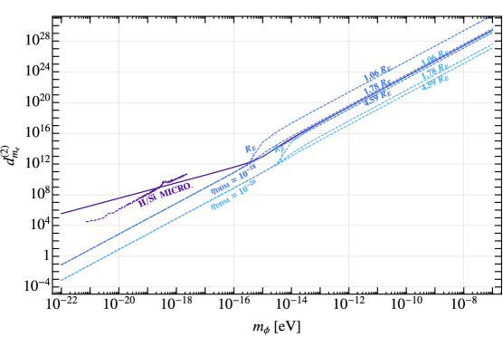
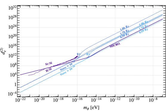
Figure 12: The bounds on the quadratic interactions with electrons (top) and photons (bottom) from a hypothetical DDM experiment done on satellites orbiting at different radii.

4 Theoretical Challenges of Models with Quadratic Couplings

In this section, we describe the theoretical issues related to theories with sizable quadratic couplings. The first is the EFT expectation setting a hierarchy between the linear and the quadratic couplings of a generic theory. The second is the naturalness problem caused by the lightness of the scalar, as a desirable large scalar quadratic coupling is associated with high corrections to the scalar mass. In Section 5, we present the symmetry principles that can give rise to a large hierarchy between linear and quadratic interactions, and in Section 6 we present a model in which in addition the scalar is kept dynamically light even for detectable quadratic couplings.

Linear vs. quadratic EFT:

Consider any naive dimension 4 (not necessarily of anomalous dimension greater than 4) SM operator, $\mathcal{O}_{\text{SM}}$. Since the action of the theory is dimensionless, any coupling between the scalar DM field and this operator has to be suppressed by some cutoff of the theory, denoted by $\Lambda$. For a linear coupling, we have only one power of $\Lambda$ suppression, $\frac{\phi}{\Lambda}\mathcal{O}_{\text{SM}}$, while for a quadratic coupling, we have two powers of $\Lambda$ suppression, $\frac{\phi^{2}}{\Lambda^{2}}\mathcal{O}_{\text{SM}}$. In the Wilsonian picture of RG, $\Lambda$ is expected to be the largest scale of the described system. As a result, we naively expect a large hierarchy between the linear and quadratic interaction strength.

Naturalness:

Consider the following interaction between the DM field and the SM fermions,

$$\mathcal{L}_{\text{int}}=\frac{d^{(2)}_{m_{e}}}{\Lambda^{2}}m_{e}\phi^{2}\psi_{e}\psi_{e}^{c}\,,\qquad\rho_{A}=\psi_{e}\psi_{e}^{c}\ \,,$$ (4.1)

where $\psi_{e}$ is the electron field. In a natural model, the quantum corrections to the mass of the light scalar, $\delta m_{\phi}^{2}$, are small compared to the classical bare mass parameter, $m_{\phi}^{2}$. The simplest 1-loop diagram that contributes to $\delta m_{\phi}^{2}$ is presented in Fig. 13.

Figure 13: 1-loop correction to the new scalar mass in the $\frac{d^{(2)}_{m_{\psi}}}{\Lambda^{2}}m_{\psi}\phi^{2}\psi\psi^{c}$ model.

Given the above electron coupling, the diagram gives the following mass correction

$$\delta(m^{2}_{\phi})^{\text{1-loop}}\sim\frac{4}{16\pi^{2}}\times\frac{d^{(2)}_{m_{e}}}{\Lambda^{2}}\left(m_{e}\Lambda^{e}_{\text{UV}}\right)^{2}\,,$$ (4.2)

where $m_{e}$ is the electron mass, and $\Lambda^{e}_{\text{UV}}$ is the effective cut-off of the loop in Fig 13, where new degrees of freedom are required to cancel the UV sensitivity of the scalar mass. The requirement $\delta m_{\phi}^{2}\lesssim m_{\phi}^{2}$ yields

$$\Lambda^{e}_{\text{UV}}\lesssim\Lambda\,\frac{2\pi}{\sqrt{d^{(2)}_{m_{e}}}}\frac{m_{\phi}}{m_{e}}\,.$$ (4.3)

For an ultra-light scalar, a measurable coupling of Eq. (4.1) requires a very small cutoff of the theory. For example, if we parameterize the experimental reach in terms of the effective temporal variation of the electron mass $\delta m_{e}/m_{e}$, induced by the ULDM field $\phi$, we find that

$$\Lambda^{e}_{\text{UV}}\lesssim\frac{2\pi}{m_{e}}\sqrt{\frac{2\rho_{\rm DM}}{\left(\delta m_{e}/m_{e}\right)^{\rm exp}}}\lesssim 20\,\,{\rm eV}\left(\frac{10^{-18}}{\left(\delta m_{e}/m_{e}\right)^{\rm exp}}\right)^{1/2}\left(\frac{\rho_{\rm DM}}{\rho_{\text{DM}}^{\odot}}\right)^{1/2}\!,$$ (4.4)

where, $\rho_{\text{DM}}^{\odot}=0.4\,{\rm GeV}/(\rm cm)^{3}$ is the mean galactic DM energy density, similar to the one expected in our solar system Salucci:2010qr , and $\left(\delta m_{e}/m_{e}\right)^{\rm exp}$ is defined as the experiment sensitivity to the variations of the electron mass. The relatively low cutoff of Eq. (4.4) is theoretically unfavorable, as it suggests that there exist some new fields with masses below $20\,{\rm eV}$ that are coupled to the SM fermions. The same analysis can be done for DM coupling to the photons, the quarks and the gluons as well. The quarks couplings yield the following bound

$$\Lambda_{\text{UV}}^{\text{q}}\lesssim\frac{2\pi}{m_{q}}\sqrt{\frac{\rho_{\rm DM}}{\left(\delta m_{q}/m_{q}\right)^{\rm exp}}}\lesssim 1\,\,{\rm keV}\left(\frac{10^{-22}}{\left(\delta m_{q}/m_{q}\right)^{\rm exp}}\right)^{1/2}\left(\frac{\rho_{\rm DM}}{\rho_{\text{DM}}^{\odot}}\right)^{1/2}\!.$$ (4.5)

Due to the difference in the degree of divergence, the parametric form of the cut-offs for the DM couplings to the photons and the gluons are different than that of Eqs. (4.4)-(4.5). For the gluon coupling, we get

$$\Lambda_{\text{UV}}^{\text{g}}\lesssim\left(8\pi^{2}\frac{\rho_{\rm DM}}{\left(\delta\alpha_{s}/\alpha_{s}\right)^{\rm exp}}\right)^{1/4}\lesssim 40\,\,{\rm keV}\left(\frac{10^{-22}}{\left(\delta\alpha_{s}/\alpha_{s}\right)^{\rm exp}}\right)^{1/4}\left(\frac{\rho_{\rm DM}}{\rho_{\text{DM}}^{\odot}}\right)^{1/4}\!.$$ (4.6)

The cutoff can be raised if the on-Earth DM density, which drives the oscillations observed in terrestrial DDM searches, is enhanced compared to the mean galactic DM density. Note that while the parameterisation above can be easily applied to any DDM experiment probing such oscillations, the effect of a DM density enhancement on the experimental sensitivity is model-dependent and experiment-dependent. One should also note that the, existence of new physics at the keV scale is constrained by various astrophysical and cosmological considerations, which are subjected to recent critical investigations Allahverdi:2020bys ; DeRocco:2020xdt . A linear coupling between the DM and the SM may also possess a naturalness problem for CP-even scalars. However, it could be protected due to the existence of accidental/non-accidental symmetries, which are absent in the case of a quadratic coupling. In addition, a CP-odd linear theory can be embedded in an axion-like theory, thus protected from a fine-tuning problem, as explained in the following section.

5 Examples of Technically-Natural Models of DM with Quadratic Interactions

In this section, we survey a few models which yield a technically-natural hierarchy between the linear ULDM coupling and the quadratic one, allowing the quadratic interactions to dominate the phenomenology of the ULDM. We begin by addressing the symmetries protecting these couplings in the agnostic EFT approach, identifying those that may retain the linear couplings small in subsection 5.1. We then specify two models in which the linear interactions are absent - a pseudo Nambu-Goldstone boson (pNGB) effective model in subsection 5.2 and a UV-complete Higgs-portal model in subsection 5.3. Finally, in subsection 5.4 we present two variations of the Clockwork framework in which the hierarchy between the linear and the quadratic couplings can be ameliorated in a technically-natural way. Although these models present theoretically-sound mechanisms for altering the naive hierarchy between the strength of the quadratic and the linear interactions, a naturally light scalar implies the quadratic interactions despite being dominant, are beyond the reach of current and near future DDM searches. We present a possible solution to this issue in Section 6.

5.1 EFT perspective of the linear vs. the quadratic couplings

In this subsection, we analyze the effective interaction between the $\phi$ sector and the SM without specifying a UV model. We consider the following three types of operators,

$$\mathcal{L}_{\text{int}}\left(\phi\right)=c_{1}^{\text{lin}}\phi\,{\cal O}_{\text{SM}}+c_{2}^{\text{lin}}\partial_{\mu}\phi\,J_{\text{SM}}^{5\mu}+c_{1}^{\text{quad}}\phi^{2}\,{\cal O}_{\text{SM}}\,.$$ (5.1)

Here we assume $\phi$ is a light pNGB and thus a pseudo-scalar, while ${\cal O}_{\text{SM}}$ is taken to be a dimension four, CP-even operator, consist of SM fields only, such as ${\cal O}_{\text{SM}}=F_{\mu\nu}F^{\mu\nu},\;m_{\psi}\psi\psi^{c}\;$etc, $J_{\text{SM}}^{5\mu}=\bar{\psi}\gamma^{\mu}\gamma^{5}\psi$ is the SM axial current. At this point, we ignore possible self coupling of $\phi$ and the possible interactions with some hidden sectors.

In general, we expect the linear $\phi$ couplings to dominate over the quadratic couplings unless the quadratic $\phi^{2}$ couplings are protected by symmetry. In this context, we consider three types of accidental symmetries that act non-trivially on the field $\phi$

$$G_{\text{global}}\supset U(1)_{\Phi}\times CP\times\mathbb{Z}_{2}^{\phi}\,.$$ (5.2)

The $U(1)_{\Phi}$ symmetry is a non-linearly realized global $U\left(1\right)$ group, which acts as a constant shift for a pNGB, thus protecting the pNGB from acquiring a mass. Thus, the smallness of the DM mass $\phi$ is protected by a shift symmetry,

$$U(1)_{\Phi}:\quad\phi\mapsto\phi+\alpha\,.$$ (5.3)

Therefore, unless the SM is charged under the $U(1)_{\Phi}$ group, both $c_{1}^{\text{lin}}\phi\,{\cal O}_{\text{SM}}$ and $c_{1}^{\text{quad}}\phi^{2}\,{\cal O}_{\text{SM}}$ breaks this symmetry. Moreover, we consider both $CP$ and $\mathbb{Z}_{2}^{\phi}$ to act similarly on the field $\phi$. $CP$ is an external symmetry with well-defined transformation rules for the SM fields, while the internal $\mathbb{Z}_{2}^{\phi}$ can be taken to affect only $\phi$. For example, we consider the action of the discrete groups as follows

$$\mathbb{Z}_{2}^{\phi}:\quad\phi\mapsto-\phi\,,$$ (5.4)

while a general CP transformation in an arbitrary basis can be written as

$$CP:\qquad\phi\left(t,\vec{x}\right) \mapsto-\phi\left(t,-\vec{x}\right)$$

$$\!\!\!\!\!\!\!\!{\cal O}_{\text{SM}}\left(t,\vec{x}\right) \mapsto{\cal O}_{\text{SM}}\left(t,-\vec{x}\right)$$ (5.5)

$$\!\!\!\!\!\!\partial_{\mu}J^{5\mu}_{\text{SM}}\left(t,\vec{x}\right) \mapsto-\partial_{\mu}J^{5\mu}_{\text{SM}}\left(t,-\vec{x}\right)\,.$$ (5.6)

Each operator in Eq. (5.1) may break one or more of the global symmetries. We summarize the symmetry breaking pattern in Table 5.

	$U\left(1\right)_{\text{shift}}$	$CP$	$\mathbb{Z}_{2}^{\phi}$
$c_{1}^{\text{lin}}\phi\,{\cal O}_{\text{SM}}$	x	x	x
$c_{2}^{\text{lin}}\partial_{\mu}\phi\,J_{\text{SM}}^{5\mu}$	$\checked$	$\checked$	x
$c_{1}^{\text{quad}}\phi^{2}\,{\cal O}_{\text{SM}}$	x	$\checked$	$\checked$

Table 5: Symmetry preserving and symmetry breaking operators.

In principle, each symmetry can be broken by a different sector. Thus, the naive expectation that the highly irrelevant operators such as $\phi^{2}\,{\cal O}_{\text{SM}}$ are less relevant than the linear ones does not hold. Moreover, the $\mathbb{Z}_{2}^{\phi}$ is considered a good approximate symmetry if the internal $\mathbb{Z}_{2}^{\phi}$ is highly protected. Thus, the quadratic coupling i.e. $c_{1}^{\text{quad}}\phi^{2}\,{\cal O}_{\text{SM}}$, can have the leading effect on the violation of EP and/or oscillations of the fundamental constants. The difference between the quadratic theory and a linear is emphasized through the analytic expressions of the EP constraints, as shown in Eq. (1.19) and Eq. (1.17). As discussed below Eq. (1.9), a quadratically coupled DM induces fundamental constants oscillations at an angular frequency of $\omega=2m_{\phi}$ compare to that of the a linear coupling such as $c_{1}^{\text{lin}}\phi{\cal O}_{\text{SM}}$ ($c_{2}^{\text{lin}}\partial_{\mu}\phi J_{\text{SM}}^{5\mu}$) which yields fundamental constant oscillations (spin precision) at an angular frequency of $\omega=m_{\phi}$. In order to be able to probe both the quadratic and the CP-even linear interaction in DDM experiments, we must require that both the couplings are not suppressed compared to one another. This criteria posses an apparent tuning problem from the perspective of a naive EFT analysis. which can be ameliorated as shown in Subsection 5.4.

5.2 A Simple pseudo-Goldstone model as a naturally ultra-light scalar DM candidate

There are several ways to avoid the naturalness requirement of a small effective cutoff. One of the most appealing solutions is to consider $\phi$ as a pNGB of some Spontaneous Symmetry Breaking (SSB). In the non-linear sigma model description of the Goldstone interactions, one must add an appropriate linear $\phi$ coupling, as well as other polynomial powers of $\phi$ interactions. The low energy theory of a spontaneous broken $U(1)_{\Phi}$ symmetry can be described by

$$\mathcal{L}_{\text{EFT}}= \,\mathcal{L}_{\text{SM}}+\frac{f^{2}}{2}\partial_{\mu}U^{\dagger}\partial^{\mu}U-m_{\psi}U\psi\psi^{c}+\frac{1}{\Lambda^{2}}\partial_{\mu}U^{\dagger}\partial^{\mu}Um_{\psi}U\psi\psi^{c}+...+\text{h.c.}\,,$$ (5.7)

where $U=e^{i\frac{\phi}{f}}$, $\psi$ is some SM fermion with mass $m_{\psi}$, $f$ is the scale at which $U(1)_{\Phi}$ is broken spontaneously, $\Lambda\gtrsim f$ is the cutoff of the theory, and the ellipsis represents higher derivatives and/or higher dimensional irrelevant operators in the Lagrangian. As shown in Eq. (5.14), the last term of Eq. (5.7) gives rise to a quadratic interaction between the SM fermions and $\phi$. This derivative term arises naturally from the low-energy physics and does not require an ad-hoc source in the UV. For example, consider a complex scalar field with a $U(1)_{\Phi}$ preserving potential

$$V(\Phi^{\dagger}\Phi)=\lambda_{\Phi}\left(\Phi^{\dagger}\Phi-\frac{f^{2}}{2}\right)^{2}.$$ (5.8)

This potential results in the SSB of the $U(1)_{\Phi}$ symmetry. Therefore, at low energies, expanding around the true vacuum of the theory, one finds a mass less Goldstone boson, $\phi$, appearing as the phase of the complex scalar as

$$\Phi=\frac{f+\rho}{\sqrt{2}}e^{i\frac{\phi}{f}}\,,~{}$$ (5.9)

where $\rho$ is the radial mode of $\Phi$ with mass $m_{\rho}\sim f$. The above parameterization manifestly provides an interaction between $\rho$ and $\phi$, which arises from the kinetic term of $\Phi$ as

$$\partial^{\mu}\Phi^{\dagger}\partial_{\mu}\Phi \simeq\partial^{\mu}\left(\frac{f+\rho}{\sqrt{2}}e^{-i\frac{\phi}{f}}\right)\partial_{\mu}\left(\frac{f+\rho}{\sqrt{2}}e^{i\frac{\phi}{f}}\right)$$

$$=\frac{1}{2}\partial_{\mu}\rho\partial^{\mu}\rho+\frac{1}{2}\partial_{\mu}\phi\partial^{\mu}\phi+\frac{1}{2f^{2}}\left(f+\rho\right)^{2}\partial_{\mu}\phi\partial^{\mu}\phi\,.$$ (5.10)

Thus, Eq. (5.10) suggests that upon integrating out the radial mode, a coupling between $\rho$ and the SM will result in a low energy effective coupling between $\partial_{\mu}\phi\partial^{\mu}\phi$ and the SM. Going back to Eq. (5.7) and expanding the exponent in terms of the small fluctuations of $\phi/f$, one finds

$$\mathcal{L}_{\text{EFT}}\supset \;\mathcal{L}_{\text{SM}}+\frac{1}{2}\partial_{\mu}\phi^{\dagger}\partial^{\mu}\phi-m_{\psi}\left(1+i\frac{\phi}{f}-\frac{\phi^{2}}{2f^{2}}+...\right)\psi\psi^{c}$$

$$+\frac{1}{m_{\rho}^{2}f^{2}}\partial_{\mu}\phi^{\dagger}\partial^{\mu}\phi m_{\psi}\left(1+i\frac{\phi}{f}-\frac{\phi^{2}}{2f^{2}}+...\right)\psi\psi^{c}+...+\text{h.c.}\,.$$ (5.11)

The corrections to $\delta m^{2}_{\phi}$ from the quadratic $\phi^{2}\psi\psi^{c}$ are exactly canceled by the corrections from the other interactions. As already mentioned, this cancellation is guaranteed by the shift symmetry of $\phi$, which is a non-linear realization of the original $U(1)_{\Phi}$ symmetry. This non-linearly $U(1)_{\Phi}$ symmetry also forbids any potential of $\phi$ as well which is manifested in a different basis. To see how it works, one can do an axial field redefinition as

$$\psi\longrightarrow e^{i\frac{\phi}{2f}}\psi\,,\qquad\psi^{c}\longrightarrow e^{i\frac{\phi}{2f}}\psi^{c}\,,$$ (5.12)

which yields the following effective Lagrangian

$$\mathcal{L}_{\text{EFT}}^{\prime}\supset\mathcal{L}_{\text{SM}}+\frac{1}{2}\partial_{\mu}\phi^{\dagger}\partial^{\mu}\phi-m_{\psi}\psi\psi^{c}-\frac{1}{f}\partial_{\mu}\phi J^{\mu}_{A}+\frac{1}{m_{\rho}^{2}f^{2}}\partial_{\mu}\phi\partial^{\mu}\phi m_{\psi}\psi\psi^{c}+...+\text{h.c.}\,,$$ (5.13)

where $J^{\mu}_{A}=\bar{\psi}\bar{\sigma}^{\mu}\partial_{\mu}\psi+\bar{\psi^{c}}\bar{\sigma}^{\mu}\partial_{\mu}\psi^{c}$ is the axial current. Note that we ignored any anomalies as these can be eliminated by an appropriate choice for the $U(1)_{\Phi}$ charges of the other fermions. Even in the absence of anomalies, the shift symmetry would be explicitly broken by a soft mass term for $\phi$, related to its nature as a DM candidate. Therefore, by using the EOM for $\phi$, one can replace, to leading order, $\partial_{\mu}\phi\partial^{\mu}\phi\rightarrow m_{\phi}^{2}\phi^{2}$, yielding an interaction term similar to the one in Eq. (4.1)

$$\mathcal{L}^{\text{nat}}_{\text{int}}=\frac{1}{\Lambda^{2}f^{2}}m_{\psi}\partial_{\mu}\phi\partial^{\mu}\phi\psi\psi^{c}\longrightarrow\frac{m^{2}_{\phi}}{\Lambda^{2}f^{2}}m_{\psi}\phi^{2}\psi\psi^{c}\,.$$ (5.14)

As expected, this implies that a natural $d^{(2)}_{m_{i}}$ coupling would be proportional to $m_{\phi}^{2}$, protecting $m_{\phi}$ against radiative corrections.
The model presented above is usually discussed in the context of ALPs. As we are interested in the (pseudo) scalar-electrons coupling, we note that it is strongly constrained by stellar evolution consideration, as those couplings provide alternative channels for stellar energy loss processes Raffelt:2012sp ; Redondo:2013lna ; Hardy:2016kme . For instance, the most stringent bound on the pseudo-scalar electron-Yukawa coupling, $\mathcal{L}\supset ig^{p}_{e}\phi\bar{\psi_{e}}\gamma^{5}\psi_{e}$, is $g_{e}^{p}\lesssim 3\times 10^{-13}\,$, obtained from the evolution of red giants Raffelt:2012sp . This can be translated to a bound on the ALP decay constant as $f\gtrsim 2\times 10^{9}\,\,{\rm GeV}\,$. The temporal oscillation of the mass of electron for an ALP decay constant allowed by cosmological consideration can be written as

$$\frac{\delta m_{e}}{m_{e}}\simeq\frac{\rho_{\rm DM}}{f^{4}}\lesssim 2\times 10^{-79}\,\left(\frac{2\times 10^{9}\,{\rm GeV}}{f}\right)^{4}\left(\frac{\rho_{\rm DM}}{\rho_{\text{DM}}^{\odot}}\right)\,,$$ (5.15)

which for detection, requires unrealistically high precision from the current and the near future DDM searches Safronova:2017xyt .

Below, we present different types of light scalar models which do not generate a linear axion-like interaction of the form $\frac{1}{f}\partial_{\mu}\phi J^{\mu}_{A}$, or in which such linear interaction is suppressed, and are thus significantly less constrained. In these models, $\phi$ mainly interacts with the SM via its quadratic derivatives. These interactions can be naturally obtained from the kinetic mixing between $\phi$ and its radial mode, as shown in Eq (5.10).

One example of such realization which leads to quadratic $\phi^{2}$ couplings without linear couplings is to consider the $\mathbb{Z}_{2}^{\phi}$ even coupling of a complex scalar field $\Phi$ as

$$\mathcal{L}_{\Phi-\rm SM}=\mathcal{L}_{\rm SM}+\partial^{\mu}\Phi^{\dagger}\partial_{\mu}\Phi+V(\Phi^{\dagger}\Phi)+16\pi^{2}\frac{\Phi^{\dagger}\Phi}{\Lambda}\psi\psi^{c}\,,$$ (5.16)

where $\psi,\psi^{c}$ are some SM fermionic fields with mass $m_{\psi}$, $\Lambda$ is the cut-off scale of the effective interaction. As explained in Section 4, imposing a $U(1)_{\Phi}$ symmetry that acts solely on $\Phi$ ensures that $\Phi$ may only couple to the SM through powers of $\Phi^{\dagger}\Phi\,\mathcal{O}^{s}_{\text{SM}}$ or higher derivative powers, where $\mathcal{O}^{s}_{\text{SM}}$ is an operator contains the SM fields which is a singlet of all SM symmetries.
Using Eq. (5.10) and the last term of Eq. (5.16), after integrating out the radial mode $\rho$ at energies below $m_{\rho}$, we get an effective interaction between $\partial_{\mu}\phi\partial^{\mu}\phi$ and the SM fermion $\psi$ as,

$$\mathcal{L}_{\rm EFT}\supset\frac{16\pi^{2}}{\Lambda m_{\rho}^{2}}\,\partial_{\mu}\phi\partial^{\mu}\phi\,\psi\psi^{c}\,.$$ (5.17)

We require that the effective cutoff would be the largest scale of the EFT, and thus

$$\Lambda\gtrsim{\rm Max}\left[4\pi f,m_{\psi}\right]\quad\Rightarrow\quad\Lambda\gtrsim{\rm Max}\left[m_{\rho},m_{\psi}\right]\,.$$ (5.18)

Note that the interaction term between the $\Phi$ sector and the SM explicitly breaks the chiral symmetry and generates a correction to the SM fermion mass at the tree-level. Assuming no fine cancellation against other contributions to the fermion mass, we require that the correction to $m_{\psi}$ from Eq. (5.16) is smaller than the physical value found in experiments. Thus,

$$\delta m_{\psi}=\frac{16\pi^{2}}{\Lambda}\frac{f^{2}}{2}\lesssim m_{\psi}\quad\Rightarrow\quad\Lambda\gtrsim\frac{16\pi^{2}\,f^{2}}{2\,m_{\psi}}\,.$$ (5.19)

By the consistency of the Goldstone theory, where $m_{\rho}\lesssim 4\pi f$, we obtain

$$\Lambda\gtrsim\frac{m_{\rho}^{2}}{2\,m_{\psi}}\,\,.$$ (5.20)

We note that if the radial mode $\rho$ is lighter than $\psi$, we expect Eq. (5.18) to give a stronger lower bound on $\Lambda$ than Eq. (5.20) as,

$$\Lambda\gtrsim{\rm Max}\left[\frac{m_{\rho}^{2}}{2\,m_{\psi}},\,\,m_{\rho}\,\,,m_{\psi}\right]\gtrsim m_{\psi}\,.$$ (5.21)

However, as the strength of the $\phi^{2}$ interactions is inversely proportional to $\Lambda$, raising the cut-off requires a higher experimental sensitivity to detect the temporal variation of $m_{\psi}$. If we parameterise the sensitivity of a DDM search experiment in terms of the variation of the electron mass $(\delta m_{e}/m_{e})$, the maximal $\Lambda$ such an experiment can probe is

$$\Lambda\lesssim 1\,\,{\rm MeV}\left(\frac{10^{-18}}{\left(\delta m_{e}/m_{e}\right)^{\rm exp}}\right)\left(\frac{30\,\,{\rm eV}}{m_{\rho}}\right)^{2}\left(\frac{\rho_{\rm DM}}{\rho_{\text{DM}}^{\odot}}\right)\,.$$ (5.22)

This translate to a bound on the mass of the radial mode, which has to satisfy

$$m_{\rho}\lesssim 45\,{\rm eV}\left(\frac{10^{-18}}{\left(\delta m_{e}/m_{e}\right)^{\rm exp}}\right)^{1/2}\left(\frac{\rho_{\rm DM}}{\rho_{\text{DM}}^{\odot}}\right)^{1/2}\!.$$ (5.23)

The characteristic sensitivity of $\left(\delta m_{e}/m_{e}\right)^{\rm exp}\sim 10^{-18}$, would allow probing models with $\rho$ as heavy as $m_{\rho}\sim 45\,\,{\rm eV}$, saturating the requirement above and a corresponding maximal cutoff of the same order. We note that an enhanced local DM density would allow DDM searches to probe models with higher cut-offs and heavier radial modes accordingly.

5.3 The Higgs-portal model - an example of a UV complete theory with no linear DM couplings

In this section, we provide an example of a specific renormalizable UV model that could result in the effective low energy SM with additional interactions of the form of Eq. (1.8). We allow other even orders of derivatives of $\phi$, such as $(\partial_{\mu}\phi\partial^{\mu}\phi)^{2}$ or $\square\phi\square\phi$, to be coupled to the SM, but forbid linear derivative couplings. To achieve the desirable low energy EFT, we extend the SM field content by introducing a new complex scalar field $\Phi$, which is a singlet of the SM gauge group. We impose an additional $U(1)_{\Phi}$ global symmetry, acting only on the $\Phi$ field, under which the SM fields are neutral.

The most general renormalizable model can be written as

$$\mathcal{L}_{\text{UV}}= \>\mathcal{L}_{\text{SM}}+\partial_{\mu}\Phi^{\dagger}\partial^{\mu}\Phi-\lambda_{\Phi H}\Phi^{\dagger}\Phi H^{\dagger}H-V(\Phi^{\dagger}\Phi)\,,$$ (5.24)

where $\mathcal{L}_{\text{SM}}$ denotes the usual SM Lagrangian, $V(\Phi^{\dagger}\Phi)$ is the potential described in Eq. (5.8) and $H$ is the SM Higgs doublet. We assume that the potential of $\Phi$ induces a SSB of the $U(1)_{\Phi}$ symmetry, upon which the low energy description of the theory is given in terms of the radial and compact modes of $\Phi$, presented in Eq. (5.9). After the electroweak symmetry breaking, the Higgs portal coupling induces an interaction between the $\Phi$ sector and the SM fermions through a mixing of the radial mode $\rho$ with the physical Higgs singlet $h$ as,

$$\mathcal{L}_{\text{H-portal}}\simeq\ -\lambda_{\Phi H}\left(\frac{f+\rho}{\sqrt{2}}\right)^{2}\left(\frac{v_{H}+h}{\sqrt{2}}\right)^{2}\,.$$ (5.25)

After diagonalizing the mass matrix $M_{\rho h}$, one obtains a $h-\rho$ mixing angle of

$$\sin\theta_{h\rho}\approx\frac{\lambda_{\Phi H}\,v_{H}\,f}{m^{2}_{h}-m^{2}_{\rho}}\,.$$ (5.26)

After integrating out $\rho$ at energy below $m_{\rho}$, we obtain interactions between $\partial_{\mu}\phi\partial^{\mu}\phi$ and the light SM fermions as discussed before. In the limit of small mixing, we obtain the following effective operator

$$\mathcal{L}_{\text{EFT}} \simeq\frac{\sin\theta_{h\rho}\,m_{\psi}}{fm^{2}_{\rho}\,v_{H}}\partial_{\mu}\phi\partial^{\mu}\phi\psi\psi^{c}=\frac{\lambda_{\Phi H}}{\left(m^{2}_{h}-m^{2}_{\rho}\right)}\frac{m_{\psi}}{m^{2}_{\rho}}\partial_{\mu}\phi\partial^{\mu}\phi\psi\psi^{c}\,,$$ (5.27)

which is shown diagrammatically in Fig. 14.

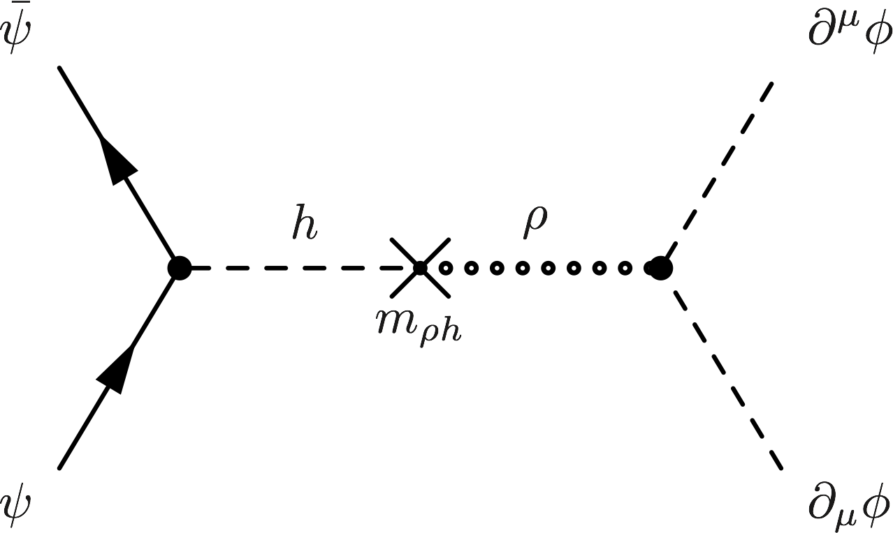
$\rightarrow$  

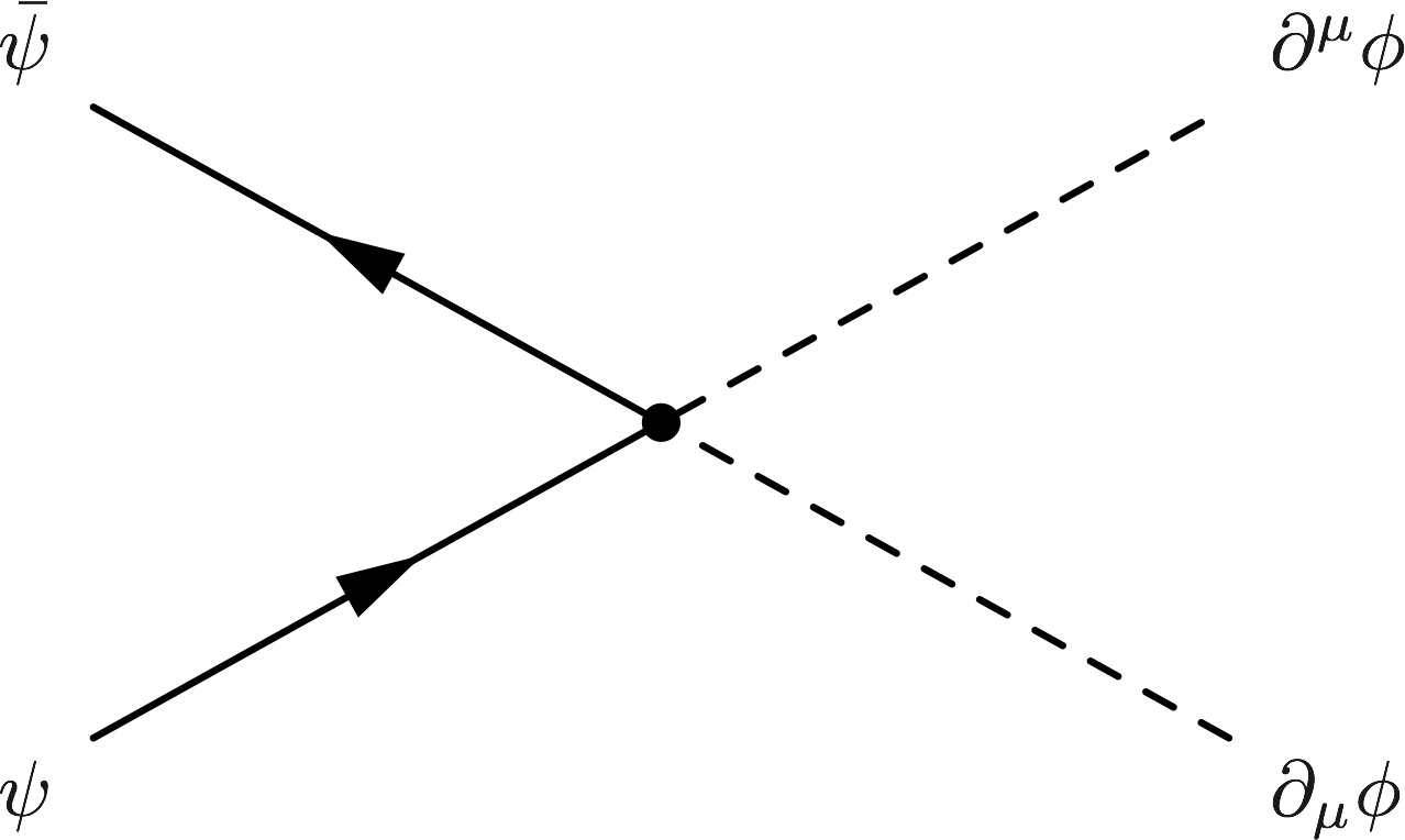
Figure 14: A diagrammatic description of the effective operator in the low energy theory.

While this model is UV complete, it sets a very low upper bound on the mass of $\rho$. In order for such a model to be detectable considering the current experimental sensitivity, the mass of the radial mode would have to be $m_{\rho}\lesssim 10^{-5}\,{\rm eV}$. While such a light invisible scalar that couples to the Higgs makes this model less appealing, we consider it to be more of a proof of concept rather than a conclusive case study. In the next subsection, we would take a more agnostic approach, studying the low-energy behavior of the natural quadratic coupling without specifying a UV completion.

5.4 The clockwork mechanism - an example of a tunable hierarchy between linear and quadratic couplings

In the previous Section 5.1, we introduced a general EFT approach to linear and quadratic couplings between the DM $\phi$ and some CP-even SM operators such as ${\cal O}_{\text{SM}}=F_{\mu\nu}F^{\mu\nu},\;m_{\psi}\psi\psi^{c}\;$ etc. We argued that different operators might break/preserve different approximate symmetries. Therefore, there could be, in principle, a large hierarchy between the dimensionless coefficient of different types of operators. For example, in some models, we expect the linear $\phi$ couplings to be suppressed and the quadratic couplings of $\phi^{2}$ to the SM to dominate the physical effects on the induced forces and potential, even though their naive dimension is higher than the linear couplings.

In this section, we provide two examples where the suppression of the linear couplings is based on symmetry principles. The examples are based on Clockwork framework Choi:2015fiu ; Kaplan:2015fuy , and the suppression is due to the existence of a large hierarchy between the effective periodicity, $F$, compare to the smaller periodicity $f$, which is the dynamical scale of a spontaneous symmetry breaking. A detailed description of the Clockwork model can be found in Appendix D.

In the Clockwork model, the remaining $U(1)_{\text{shift}}$ symmetry, which keeps the DM mass small, is identified with the remaining $U\!\left(1\right)_{\text{clock}}$ of the N+1 Clockwork model, as shown in Eq. (D.8) where $N$ is the number of Clockwork sites. Note that in the limit of exact $U(1)_{\text{shift}}$ symmetry, $\phi$ is mass-less. In order to achieve suppression of the linear $\phi$ couplings, we assign small charges to the SM fermions, i.e., $[\psi]\sim\mathcal{O}(1)$, such that the leading symmetry preserving interaction is on the last Clockwork site,

$$\mathcal{L}_{\text{int}}^{\text{leading}}\supset c_{N}\frac{\Phi_{N}}{\Lambda}LHE^{c}+V_{\text{mixing}}\left(\Phi_{N},H\right)+\text{h.c.}\,,$$ (5.28)

where $L$ are the left-handed $SU(2)$ doublet SM Lepton fields, while $E^{c}$ are the left-handed $SU(2)$ singlet SM Lepton fields. We assume that $V_{\text{mixing}}\left(\Phi_{N},H\right)$ breaks CP spontaneously by some parameter $\theta_{\text{CP}}\ll 1$, which is defined as the CP mixing angle between the Clockwork and the Higgs CP eigenstates:

$$\phi= \cos\theta_{\text{CP}}\hat{\phi}+\sin\theta_{\text{CP}}\hat{h}\,,$$ (5.29)

$$h= -\sin\theta_{\text{CP}}\hat{\phi}+\cos\theta_{\text{CP}}\hat{h}\,.$$ (5.30)

$V_{\text{mixing}}\left(\Phi_{N},H\right)$ can give rise to both CP-even and CP-odd interactions between $\phi$ and the SM fields.

At low energies, we can integrate out the heavy modes of the Clockwork and obtain an effective Lagrangian of the pNGB which is identified as the ULDM field,

$$\mathcal{L}_{\text{EFT- int}}^{\text{leading}}\supset c_{N}\frac{f\,e^{i\frac{\phi}{F}}}{\Lambda}h\psi\psi^{c}+V_{\text{mixing}}\left(\frac{\phi}{F},H\right)+\text{h.c.}\,,$$ (5.31)

where $c_{N}$ is some $\mathcal{O}(1)$ coefficient. As a result, the derivative coupling of $\phi$, of the form $\frac{f}{\Lambda}\frac{\partial_{\mu}\phi}{F}m_{\psi}\left[\bar{\psi}\bar{\sigma}^{\mu}\psi-\bar{\psi}^{c}\bar{\sigma}^{\mu}\psi^{c}\right]$, is highly suppressed by $F=3^{N}f$.

The higher dimensional operator

$$\mathcal{L}_{\text{int}}^{\text{NL}}\supset c_{0}\frac{\Phi_{0}^{\dagger}\Phi_{0}}{\Lambda^{2}}m_{\psi}\psi\psi^{c}+\text{h.c.}\,,$$ (5.32)

gives rise to a quadratic coupling that is only suppressed by $f$, not $F$. $c_{0}$ is some $\mathcal{O}(1)$ coefficient. After integrating out the heavy Clockwork radial modes, from Eq. (5.32) we obtain,

$$\mathcal{L}_{\text{EFT- int}}\supset c_{0}\frac{1}{2f^{2}\Lambda^{2}}\partial_{\mu}\phi\partial^{\mu}\phi\,m_{\psi}\psi\psi^{c}\,.$$ (5.33)

Since $F=3^{N}f$, is just an artifact scale of the Clockwork model, it can be larger than the cutoff scale, $\Lambda\gtrsim f$. Thus, we achieve a hierarchy between the linear and the quadratic (dimensionless) couplings.

Moreover, adding the both the interactions of Eq. (5.28) and Eq. (5.32) leads to a collective breaking of the $U\!\left(1\right)_{\text{clock}}$ symmetry. As a result, one can write the effective potential generated for this pNGB. The 1-loop Coleman-Weinberg (CW) effective potential of $\phi$ can be written as,

$$\!\!\!\!V_{\text{CW}}\left(\phi\right)=\frac{\left(-1\right)^{\mathcal{F}}}{64\pi^{2}}Tr\left[2M^{\dagger}\left(\phi\right)M\left(\phi\right)\Lambda_{c}^{2}+\left(M^{\dagger}\left(\phi\right)M\left(\phi\right)\right)^{2}\ln\frac{M^{\dagger}\left(\phi\right)M\left(\phi\right)}{\tilde{\Lambda}_{c}^{2}}\right]\!.\!\!$$ (5.34)

In the equation above, Tr is performed over all field degrees of freedom, $(-1)^{\mathcal{F}}$ is $+1$ for bosons and $-1$ for fermions. The momentum cutoff $\Lambda_{c}$, is taken to be of the order of the radial mode mass, which is of $\mathcal{O}(f)$. Thus, at the leading order the effective potential of $\phi$ can be approximately written as

$$V(\phi)\simeq-c_{0}c_{N}\frac{m_{\psi}^{2}f^{3}}{16\pi^{2}\Lambda}\cos\left(\frac{\phi}{F}\right).$$ (5.35)

The induced DM potential of Eq. (5.35) generates a contribution to the DM mass of

$$m_{\phi}^{2}\simeq c_{0}c_{N}\frac{m_{\psi}^{2}f^{3}}{16\pi^{2}\Lambda}\frac{1}{F^{2}}\,.$$ (5.36)

Therefore, if Eq. (5.35) is the only source of the DM mass, the quadratic interaction will also be suppressed by $1/F^{2}$, and similar to the linear interaction. Therefore, we require that there is an additional source of the DM mass, $m_{\phi}^{2}$ which is not suppressed by $1/F^{2}$.

Another way to employ the Clockwork mechanism is one where the shift symmetry is broken at the two ends of the Clockwork chain i.e. at the first site, at $\Phi_{0}$, and at the last site, at $\Phi_{N}$. We assume two different $Z_{2}$ symmetries are conserved in each site, such that the Lagrangian of these $U(1)_{\text{clock}}$ breaking sectors can be written as,

$$\mathcal{L}_{\text{int}}^{\text{leading}}\supset c_{N}\frac{\Phi_{N}-\Phi_{N}^{\dagger}}{\Lambda}m_{\psi}\psi\psi^{c}+c_{0}\frac{\Phi_{0}+\Phi_{0}^{\dagger}}{\Lambda}m_{\psi}\psi\psi^{c}\,.$$ (5.37)

Therefore, the effective Lagrangian of the pNGB takes the form of

$$\mathcal{L}_{\text{effective}}^{\text{leading}}\simeq c_{N}\frac{f\sin\left(\frac{\phi}{F}\right)}{\Lambda}m_{\psi}\psi\psi^{c}+c_{0}\frac{f\cos\left(\frac{\phi}{f}\right)}{\Lambda}m_{\psi}\psi\psi^{c}\,.$$ (5.38)

Assuming the clockwork potential is dominated by a backreaction potential which has a minimum near $\phi\simeq 0$, one can expand the trigonometric functions to achieve the desired hierarchy between the linear coupling and the quadratic coupling, relatively suppressed by $f/F\ll 1$, as

$$\mathcal{L}_{\text{effective}}^{\text{leading}}\simeq\frac{c_{N}\,f}{\Lambda F}\phi m_{\psi}\psi\psi^{c}+\frac{c_{0}}{\Lambda f}\phi^{2}m_{\psi}\psi\psi^{c}\,.$$ (5.39)

6 Sensible Models of Light Scalars with Large Quadratic Couplings

As mentioned in previous sections, we are interested in keeping the scalar naturally light, while also maintaining its quadratic interactions within experimental reach. This should be achieved in conjunction to ensuring that the linear scalar interactions are suppressed. In this section we shall consider two main constructions that realize such a scenario. We begin by briefly reviewing the idea presented in Hook:2018jle , which involves a QCD axion with a $\mathbb{Z}_{N}$ symmetry acting on $N$ copies of the SM. We then move to describe a realization of the relaxed-relaxion idea Banerjee:2020kww , that shows that relaxion models may yield naively unnaturally-large couplings for a light relaxion.

6.1 Quadratic interactions of the naturally light $\mathbb{Z}_{N}$ QCD-axion

It is interesting to note that there is a class of models that naturally leads to sizeable quadratic interactions between the ULDM and the SM field, with no corresponding linear scalar coupling. This is precisely the effective theory of a certain kind of a naturally light QCD-axion model, where the axion mass is suppressed relative to the conventional models due to the presence of $N$ copies of the SM, which furnish a $\mathbb{Z}_{N}$ symmetry Hook:2018jle ; DiLuzio:2021pxd  . In this class of models, while the axion couplings to the SM fields (our SM) follow the conventional models, the axion mass is suppressed by an additional factor of $z^{N}$, with $z\equiv m_{u}/m_{d}\sim 1/2$ given by the up to down quark mass ratio. Furthermore, as was demonstrated in Kim:2022ype , while at linear order, the axion couplings to the SM fields are only to pseudo-scalar operators (thus preserving parity), the axion also possesses quadratic couplings to the hadrons. This leads to exciting phenomenology as the QCD axion can be searched for in experiments that consider the variation of coupling constants instead of the conventional QCD-axion searches (see e.g. Graham:2013gfa ). For more information, we refer the reader to Kim:2022ype .

6.2 Quadratic interactions of a light relaxed-relaxion

Another possibility to ameliorate the naturalness bound for a light scalar is by relaxing its mass in a dynamical way Banerjee:2020kww ; Banerjee:2022wzk . Dynamical relaxation of a light scalar is discussed in the context of the relaxion mechanism Graham:2015cka , where the light scalar field scans the Higgs mass parameter starting from some high cut-off down to its measured value. As discussed Banerjee:2020kww , due to the small incremental change of the Higgs VEV as a function of the scalar field value, the scalar stops at a shallow part of its potential and the stopping point (in the field space) is very close to $\phi/f\sim\pi/2$. As a result of the shallowness of the scalar’s potential, its mass is suppressed compare to the naive expected value, however the interaction strength with the Higgs/SM is not. Thus for low energy observers, the scalar appears to be unnatural although the relaxion mechanism is constructed in a technically-natural way.

Below we use a similar idea in order to suppress the mass of the ULDM field, while maintaining its quadratic interactions observable and suppressing its linear interactions with the SM. To achieve that we relax the mass of a hidden sector Higgs, $\hat{H}$, from some cut-off $\Lambda$ to its true VEV $\hat{v}$, and invoke an interaction of the scalar with the SM as given in Eq. (6.1).

6.2.1 Interaction with the SM

We assume that the field $\phi$ is coupled to the light SM matter as

$$\mathcal{L}_{\text{int }}\supset-\sin\left(\frac{\phi}{f}\right)\left[\sum_{\psi=e,u,d}g_{\phi\psi}m_{\psi}\psi\psi^{c}+\frac{g_{\phi\gamma}}{2}F_{\mu\nu}F^{\mu\nu}+\frac{g_{\phi g}}{2}G_{\mu\nu}G^{\mu\nu}+\text{h.c.}\right]\,,$$ (6.1)

which can be obtained by demanding that the UV completion of this sector includes a linear complex field $\Phi=\left(\rho+f\right)\exp\left(i\frac{\phi}{f}\right)$, and respects a version of charge conjugation under which $\Phi\rightarrow-\Phi^{*}$. At leading order, Eq. (6.1) generates a quadratic coupling to the light matter in a technically natural way. We can calculate the 1-loop potential of $\phi$, generated by the diagrams presented in Fig. 15, similarly to Eq.(5.34), as

$$V\left(\phi\right)\simeq\frac{1}{16\pi^{2}}\left[\!\sum_{\psi=e,u,d}\!\!\!2\,g_{\phi\psi}\,m_{\psi}^{2}\Lambda_{\rm cut}^{2}\!\left[\sin\left(\frac{\phi}{f}\right)\!+\!g_{\phi\psi}\sin^{2}\left(\frac{\phi}{f}\right)\right]\!\!+\!\!\sum_{A=\gamma,g}\!\!g_{\phi A}\Lambda_{\rm cut}^{4}\sin\left(\frac{\phi}{f}\right)\!\right]\!,$$ (6.2)

where $\Lambda_{\rm cut}\gtrsim m_{e}$ is the momentum cut-off of the loop. The overall potential for $\phi$ can be written as,

$$V(\phi,\hat{H}) =-g\Lambda^{3}\phi+\left(\Lambda^{2}-g\Lambda\phi-\mu_{\rm br}^{2}\cos\frac{\phi}{f}\right)|\hat{H}|^{2}+|\hat{H}|^{4}$$

$$+\frac{1}{8\pi^{2}}\,\sum_{\psi=e,u,d}g_{\phi\psi}m^{2}_{\psi}\Lambda_{\rm cut}^{2}\,\sin\frac{\phi}{f}+\frac{1}{16\pi^{2}}\sum_{A=\gamma,g}g_{\phi A}\Lambda_{\rm cut}^{4}\sin\frac{\phi}{f}\,,$$ (6.3)

$\hat{H}$ belongs to a new hidden sector whose mass is being relaxed from some cut-off $\Lambda$ to its true vacuum expectation value $\hat{v}=\left<\hat{H}\right>$, $g$ is small theory parameter and $\mu_{\rm br}\lesssim\hat{v}$ is the scale of the cosine potential (for more details of this kind of construction see e.g. Graham:2015cka ; Banerjee:2020kww ).

+

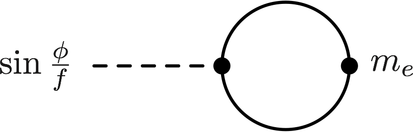
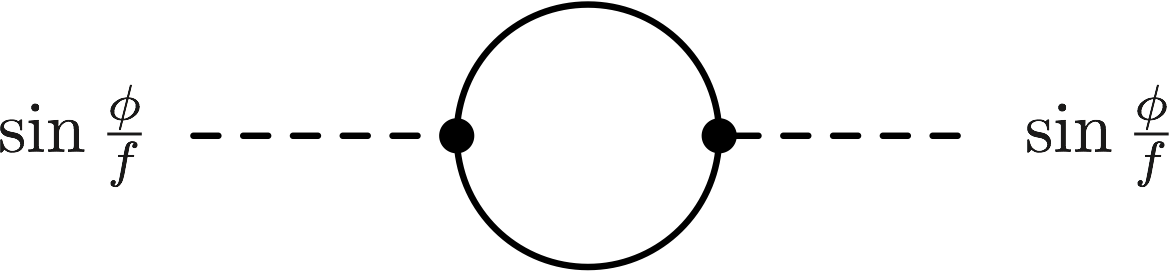
Figure 15: Feynman diagrams for generating Coleman Weinberg for $\phi$ at 1-loop order coming from Eq. 6.1.

To achieve a successful relaxation of the mass parameter of $\hat{H}$, we require

$$\mu_{\rm br}^{2}\hat{v}^{2}\gtrsim\frac{1}{8\pi^{2}}\,g_{\phi\psi}\,m_{\psi}^{2}\,\Lambda_{\rm cut}^{2}\,.$$ (6.4)

Minimizing Eq. (6.3) with respect to both $\hat{H}$ and $\phi$, and using the above constraint, we find the field stopping point as

$$\frac{\phi_{0}}{f}\simeq\frac{\pi}{2}-\frac{\mu_{\rm br}^{2}}{2\hat{v}^{2}}-\frac{g_{\phi\psi}\,m_{\psi}^{2}\,\Lambda_{\rm cut}^{2}}{8\pi^{2}\mu_{br}^{2}\hat{v}^{2}}\pm\frac{\mu_{\rm br}}{\Lambda}\equiv\frac{\pi}{2}-\delta_{\pi/2}\,,$$ (6.5)

where $\delta_{\pi/2}\ll 1$ is defined as the deviation from $\pi/2$. As explained in Banerjee:2020kww , we obtain the mass of the light scalar $\phi$ as,

$$m_{\phi}^{2}\approx\frac{\mu_{\rm br}^{2}\hat{v}^{2}}{f^{2}}\frac{\mu_{\rm br}}{\Lambda}=\frac{\mu_{\rm br}^{2}\hat{v}^{2}}{f^{2}}\delta\,,$$ (6.6)

which is suppressed compare to the naive expected value of $m_{\rm naive}^{2}\sim\mu_{\rm br}^{2}\hat{v}^{2}/f^{2}$ by a small parameter defined as $\delta=\mu_{\rm br}/\Lambda\ll 1$. This suppression is a result of the flatness of the effective potential of $\phi$, which characterizes the first point at which the derivative of the backreaction potential, mainly controlled by a periodic function of $\phi$ with a slowly rising amplitude, balances out the constant derivative of the UV term.

Expanding Eq. (6.1) around the stopping point of $\phi$ gives rise to linear and quadratic couplings of $\phi$ to the SM as

$$\mathcal{L}_{\rm int}\supset -\sum_{\psi=e,u,d}g_{\phi\psi}m_{\psi}\psi\psi^{c}\left(1-\frac{\delta_{\pi/2}^{2}}{2}-\frac{\phi^{2}}{2f^{2}}-\delta_{\pi/2}\frac{\phi}{f}\right)$$

$$+\left[\frac{g_{\phi\gamma}}{2}F_{\mu\nu}F^{\mu\nu}+\frac{g_{\phi g}}{2}G_{\mu\nu}G^{\mu\nu}\right]\left(1-\frac{\delta_{\pi/2}^{2}}{2}-\frac{\phi^{2}}{2f^{2}}-\delta_{\pi/2}\frac{\phi}{f}\right)\,.$$ (6.7)

Moreover, for a valid weakly coupled theory, we require

$$\delta m_{\psi}\lesssim m_{\psi}\qquad\text{ i.e}\>g_{\phi\psi}\lesssim\mathcal{O}(1)\,,$$ (6.8)

$$\delta\alpha_{(s)}\lesssim\alpha_{(s)}\qquad\!\!\text{i.e. }\>g_{\phi\gamma(g)}\lesssim\mathcal{O}(1)\,.$$ (6.9)

Combining Eq. (6.4) and Eq. (6.9) we get

$$g_{\phi\psi}\lesssim{\rm Min}\left[1,8\pi^{2}\frac{\mu_{\rm br}^{2}\hat{v}^{2}}{m_{\psi}^{2}\,\Lambda^{2}}\right]\,,$$ (6.10)

$$g_{\phi\gamma(g)}\lesssim{\rm Min}\left[1,4\pi^{2}\frac{\mu_{\rm br}^{2}\hat{v}^{2}}{\Lambda^{4}}\right]\,.$$ (6.11)

6.2.2 Relaxation of the cutoff

Consider a model where the field stopping point is not near $\phi_{0}/f\sim\frac{\pi}{2}$ as in Eq. (6.5), but a naive order one stopping point,

$$\left(\frac{\phi_{0}}{f}\right)_{\text{Naive}}\sim\mathcal{O}(1)\,.$$ (6.12)

For simplicity, let us focus on the quadratic coupling of $\phi$ to the electron

$$\mathcal{L}\supset g_{\phi e}\frac{\phi^{2}}{f^{2}}\,m_{e}\,ee^{c}\,.$$ (6.13)

Given the naive stopping point, this interaction leads to a quadratic contribution to the scalar mass as

$$\left(\delta m_{\phi}^{2}\right)_{\text{Naive}}\simeq g_{\phi e}\,m_{e}^{2}\,\frac{\Lambda_{e}^{2}}{8\pi^{2}f^{2}}\,,$$ (6.14)

where $\Lambda_{e}$ is the cut-off of the electron loop. In addition, if the scalar field $\phi$ accounts for the DM in the present universe, it acquires a time-dependent background value. Thus, the same coupling would induce temporal variations of the mass of the electron as

$$\frac{\delta m_{e}}{m_{e}}(t)\simeq g_{\phi e}\frac{\rho_{\rm DM}}{f^{2}m_{\phi}^{2}}\,.$$ (6.15)

We then obtain a simple relation between the variation of the fundamental constant and the correction to the mass of $\phi$

$$\left(\delta m_{\phi}^{2}\right)_{\text{Naive}}=\left(\frac{\delta m_{e}}{m_{e}}\right)(t)\times\frac{m_{e}^{2}\,m_{\phi}^{2}\,\Lambda_{e}^{2}}{\rho_{\rm DM}\,8\pi^{2}}\,.$$ (6.16)

Without the relaxed relaxion dynamics, a theory involving such interactions can only be natural if

$$\left(\delta m_{\phi}^{2}\right)_{\text{Naive}}\lesssim m_{\phi}^{2}\Rightarrow\frac{\delta m_{e}}{m_{e}}(t)\times\frac{\Lambda_{e}^{2}}{8\pi^{2}}\lesssim\frac{\rho_{\rm DM}}{m_{e}^{2}}\,.\\$$ (6.17)

Thus, naively, theories of natural light scalars generating observable variations of constants of nature would imply new physics should appear at relatively low scales as

$$\Lambda_{e}\lesssim 30\,{\rm eV}\,\left(\frac{\rho_{\rm DM}}{\rho_{\rm DM}^{\odot}}\right)^{1/2}\left(\frac{10^{-18}}{\left(\delta m_{e}/m_{e}\right)^{\rm exp}}\right)^{1/2}.$$ (6.18)

In light of this consideration, we can determine whether a theory described by Eq. (6.3) is natural or unnatural, by quantifying by how much the cut-off of the theory is being relaxed away from the naive estimation above.

In the relaxed scenario, the 1-loop order corrections to the mass of $\phi$ are already taken into account via the effective potential in Eq. (6.3), yielding the stopping point given in Eq. (6.5), and the suppressed mass in Eq. (6.6). Therefore, naturalness does not require that these 1-loop corrections are kept smaller than $m_{\phi}$. However, for the relaxation to be successful (both of the mass of $\hat{H}$ and of the mass of $\phi$), we must require that the coupling of $\phi$ to the SM does not overcome the derivative of the $\hat{H}$-dependent potential of $\phi$ at the first stopping point. This requirement is expressed in Eq. (6.4), and can be re-expressed as

$$\frac{{g}_{\phi e}\,m_{e}^{2}\,\Lambda_{e}^{2}}{8\pi^{2}f^{2}}\lesssim\frac{\mu_{\rm br}^{2}\hat{v}^{2}}{f^{2}}\,,$$ (6.19)

or

$$\left(\delta m_{\phi}^{2}\right)_{\rm{Naive}}\lesssim\frac{m_{\phi}^{2}}{\delta}\,,$$ (6.20)

which is less restrictive than the naive requirement in Eq. (6.17) since $\delta\lesssim 1$. Consequently, the phenomenological effects associated with the coupling of $\phi$ to the SM may be enhanced, without significantly altering the mass of the scalar. Namely, the cut-off scale of such a theory $\Lambda_{e}$, including a light scalar and observable quadratic interactions with the SM, is relaxed by a factor of $1/\sqrt{\delta}$ with respect to the naive prediction of Eq. (6.18).

6.2.3 A large hierarchy between the linear and quadratic coupling due to the Relaxed Relaxion mechanism

A large hierarchy between the effective linear and quadratic couplings of $\phi$ can be simply parameterize in terms of the deviation of the scalar’s stopping point from $\frac{\pi}{2}$, denoted by $\delta_{\pi/2}$. The different scaling between the dimensionless linear and quadratic couplings is

$$c_{\text{linear}}\sim g_{\phi(\psi,A)}\times\delta_{\pi/2},\qquad\text{while}\qquad c_{\text{quadratic}}\sim g_{\phi(\psi,A)}\,.$$ (6.21)

In our natural theory we consider $g_{\phi(\psi,A)}\sim\mathcal{O}\left(1\right)$. Moreover, we wish to have natural values of the scaled couplings, which gives new bounds that are absent if only either the linear or the quadratic coupling were to be turned on. For example, in order to match the observed bound of $d_{m_{e}}^{\left(2\right)}\sim 10^{14}$, one must require that

$$\mathcal{O}(1)\sim c_{m_{e}}^{\left(2\right)}=d_{m_{e}}^{\left(2\right)}\times\frac{f^{2}}{M_{\text{pl}}^{2}}\simeq\frac{f^{2}}{\text{GeV}^{2}}\times 10^{-23}\;\Rightarrow\;f\simeq 3\times 10^{11}\,\text{GeV}\,,$$ (6.22)

in order to get $\mathcal{O}(1)$ coupling. This, in turn, sets the value of the relaxion dynamical scale, $f$. For the linear coupling, matching the observed bound on $d_{m_{e}}^{\left(1\right)}\sim 10^{-3}$ translates to

$$c_{m_{e}}^{\left(1\right)}=d_{m_{e}}^{\left(1\right)}\times\frac{f}{M_{\text{pl}}}\simeq 10^{-10}\sim\delta_{\pi/2}$$ (6.23)

which sets the value of $\delta_{\pi/2}$. Assuming no cancellation between the different terms contributing to $\delta_{\pi/2}$, we get the following constraints:

$$\begin{cases}\frac{\mu_{{\rm br}}^{2}}{\hat{v}^{2}}\lesssim 10^{-10}\,\\ \frac{\mu_{{\rm br}}}{\Lambda}\lesssim 10^{-10}\,\\ \frac{g_{\phi\psi}\,m_{\psi}^{2}\,\Lambda_{\rm cut}^{2}}{8\pi^{2}\mu_{br}^{2}\hat{v}^{2}}\lesssim 10^{-10}\,.\end{cases}$$ (6.24)

The first two constraints from Eq. (6.24) can be easily satisfied by constructing $\mu_{{\rm br}}\ll\hat{v},\Lambda$. The last constraint from Eq. (6.24) can also be achieved. However, it suggests that it is more likely to see an effect of both linear and quadratic couplings to light SM matter.

An example of the allowed parameter space for this model, including the theoretical considerations above as well as the experimental bounds, is presented in Fig 16 for a fixed $f=10\,\hat{v}=10^{7}\,\text{GeV}$ and a cutoff of $\Lambda_{e}=10\,\text{MeV}$. We plot both the bounds on the quadratic coupling and on the linear coupling (for a generic $\mathcal{O}\left(1\right)$ stopping point and for the relaxed-relaxion mechanism) separately, however, since they are not independent in this model, the bound should be drawn from satisfying these constraints simultaneously (shaded lilac region of Fig. 16). This yields non-trivial constraints both due to the interdependence of these couplings in this model, making it impossible to turn off the quadratic coupling without turning off the linear coupling as well, and also taking into account the non-linear effects discussed in subsection 3.1. Note that the EP constraints involving the quadratic coupling strongly depend on the radius of the source $R_{C}$ and on the distance from the center of the source $r$. Our bounds are calculated assuming $R_{C}=r=R_{\oplus}$ for Eöt-Wash Be/Ti Schlamminger:2007ht and $R_{C}=R_{\oplus}\,,r=R_{\oplus}+700$  km for MICROSCOPE PhysRevLett.129.121102 , with $R_{\oplus}$ being the radius of the Earth. Although we have focused on the electron coupling $g_{\phi e}$, the same analysis can be easily extended to other couplings between $\phi$ and the SM fields, such as $g_{\phi\gamma},g_{\phi u(d)}$ and $g_{\phi g}$.

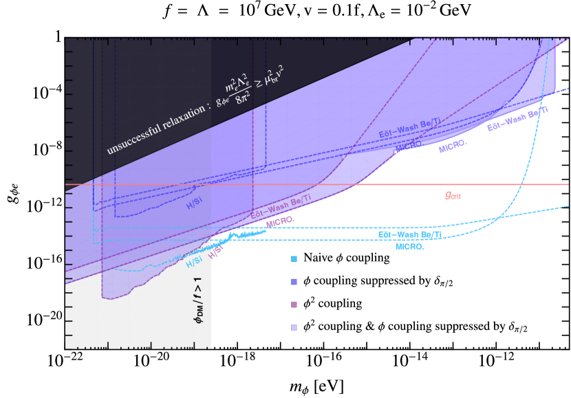
Figure 16: The allowed parameter space of an ULDM relaxed-relaxion inspired model with $f=\Lambda=10\,\hat{v}=10^{7}\text{\,GeV}$, and $\Lambda_{e}=10\,\,{\rm MeV}$. Blue - bounds on a model with only the suppressed linear coupling given, purple - bounds on a model with only the quadratic coupling, light blue - bounds on a model with a naive linear coupling, lilac - bounds given by the combination of the quadratic coupling and the suppressed linear coupling. Pink - the critical coupling for the quadratic interactions. Black - the region in which there is no relaxation of the mass parameter of $\hat{H}$, gray - region in which the ULDM amplitude is greater than $f$.

7 Conclusions

In this work, we considered a special class of spin-0 ULDM models. In this class, the dominant operators describing the interactions between the ULDM field $\phi$ and the SM are quadratic in the ULDM field, namely, of the form $\phi^{2}\mathcal{O}_{\rm SM}$ where $\mathcal{O}_{\rm SM}$ composed of SM fields.

A dominant quadratic interaction between the ULDM field and the SM poses two problems to a quantum field theory. First, naive EFT power counting suggests that linear ULDM couplings would dominate over the quadratic couplings, as the former are associated with effective operators of lower mass-dimensions. Second, generic quadratic interactions generate a large additive contribution to the mass of the ULDM, thus resulting in a naturalness problem. We discussed theoretical constructs in which these challenges are ameliorated. First, we presented technically-natural models where the dominant interaction between the ULDM and the SM is in fact quadratic with the ULDM field, and the linear (scalar) coupling is either absent or suppressed. Second, with a $\mathbb{Z}_{N}$ QCD axion model and a relaxed-relaxion inspired framework, we demonstrated that a large quadratic coupling and a parametrically smaller mass can be achieved naturally.

We have also studied the phenomenology of this class of models, considering various terrestrial and space-based existing and near future experimental probes. Finally, we considered the interplay between indirect searches for the ULDM field, related to tests of the violation of the EP and the existence of the fifth-force, and the direct searches associated with temporal oscillations of the fundamental constants of nature.

Appendix A The EOM of DM for Linearly Coupled model

Let us consider a linearly coupled CP-even scalar DM with the SM described by Eq. (1.2). The EOM for the DM field $\phi$ can be written as,

$$\left(\frac{\partial^{2}}{\partial t^{2}}-\nabla\cdot\nabla+m_{\phi}^{2}\right)\phi=J_{\text{source}}\left(r\right)\,,$$ (A.1)

where $J_{\text{source}}\left(r\right)\equiv-\frac{Q^{C}_{i}d_{i}^{\left(1\right)}}{M_{\text{Pl}}}\rho_{C}\left(r\right)$ is coming because of the presence of a source term with density $\rho_{C}$ and dilatonic $Q_{i}^{C}$ are the dilatonic charges for the body C, corresponding to the i-th fundamental constant (and corresponding coupling). We consider a homogeneous spherically symmetric source satisfies

$$\rho_{C}\left(r\right)=\begin{cases}\frac{3M_{C}}{4\pi R_{C}^{3}}&r\leq R_{C}\\ 0&r>R_{C}\,,\end{cases}$$ (A.2)

where $M_{C}$ and $R_{C}$ are the mass and the radius of the body C. The solution to the EOM for the scalar field $\phi$, in the presence of a homogeneous spherical source, is

$$\phi\left(t,x\right)=\phi_{0}\cos\left(m_{\phi}t+\delta\right)-\frac{Q^{C}_{i}d_{i}^{\left(1\right)}}{M_{\text{Pl}}}\,I\left(m_{\phi}R_{C}\right)\frac{M_{C}}{r}\,e^{-m_{\phi}r}\,,$$ (A.3)

where the function $I\left(x\right)$ is given by

$$I\left(x\right)=3\dfrac{x\cosh x-\sinh x}{x^{3}}\>=\begin{cases}1&x\ll 1\\ \frac{e^{x}}{2x}&x\gg 1\,,\end{cases}$$ (A.4)

and $\phi_{0}=\sqrt{2\rho_{\rm DM}}/m_{\phi}$, and $\delta$ is a random phase of the DM background. $\rho_{\rm DM}$ is the local DM density. The sensitivity of EP tests can be written as (Eq. (1.17) in the main text)

$$\eta^{\text{EP}}_{\rm lin}=2\frac{|\vec{a}_{A,C}-\vec{a}_{B,C}|}{|\vec{a}_{A,C}+\vec{a}_{B,C}|} \approx\frac{|\left(Q_{i}^{A}d^{(1)}_{i}-Q_{i}^{B}d^{(1)}_{i}\right)\vec{\nabla}V_{C}\left(\phi\right)|}{\frac{GM_{C}}{r^{2}}}$$

$$\simeq Q^{C}_{j}d^{(1)}_{j}{\left(Q_{i}^{A}d^{(1)}_{i}-Q_{i}^{B}d^{(1)}_{i}\right)}e^{-m_{\phi}r}\,.$$ (A.5)

Having a time-varying background field, as in Eq. (A.3), induces a small temporal dependence of fundamental constants which can be probed by DDM searches. In DDM searches, we compare two systems (say A and B) with sensitivity coefficients $\kappa^{A/B}_{i}$ corresponding to the i-th fundamental constant. The sensitivity of the DDM searches can be written as (Eq. (1.18) in the main text)

$$\eta^{\text{DDM}}_{\rm lin}=\frac{|\delta Y(t)|}{Y}\approx\frac{\Delta\kappa_{i}d_{i}^{(1)}}{M_{\text{Pl}}}\phi_{0}\,\cos\left(m_{\phi}t+\delta\right)\,,$$ (A.6)

where $\Delta\kappa_{i}=\kappa^{A}_{i}-\kappa^{B}_{i}$ is the difference of the sensitivity coefficients of a specific transition.

Appendix B The EOM of a Quadratically Coupled DM Model

The EOM for the DM field in the quadratic model, described by Eq. (1.8), is

$$\left(\frac{\partial^{2}}{\partial t^{2}}-\nabla\cdot\nabla+\tilde{m}_{\phi}^{2}\left(r\right)\right)\phi=0\,,$$ (B.1)

where we define $\tilde{m}_{\phi}^{2}\left(r\right)\equiv m_{\phi}^{2}+\frac{Q_{i}^{C}d_{i}^{(2)}}{M_{\text{Pl}}^{2}}\rho_{C}\left(r\right)$. We also replace the SM matter fields, with the background source density, $\rho_{C}\left(r\right)$, in the presence of a spherically homogeneous source as described in Eq. (A.2).

The EOM yields a solution outside the source body of the form

$$\phi\left(t,x\right)=\phi_{0}\cos\left(m_{\phi}t+\delta\right)\left[1-s_{C}^{\left(2\right)}[d^{(2)}_{i}]\,\frac{GM_{C}}{r}\right]\,.$$ (B.2)

In the above equation, $C$ stands for the source body with

$$s^{(2)}_{C}[d^{(2)}_{i}]=Q^{C}_{i}d^{(2)}_{i}J_{\textrm{sign}[d^{(2)}_{i}]}\left(\sqrt{3Q^{C}_{i}d^{(2)}_{i}\frac{GM_{C}}{R_{C}}}\right)\,,$$ (B.3)

where the function $J_{\textrm{sign}[d^{(2)}_{i}]}\left(x\right)$ is defined in Hees:2018fpg as

$$J_{+}(x)=3\frac{x-\tanh x}{x^{3}}\,\,\,{\rm and}\,\,\,J_{-}(x)=3\frac{\tan x-x}{x^{3}}\,.$$ (B.4)

Note that, we consider the case where all the couplings are positive i.e. $\textrm{sign}[d^{(2)}_{i}]\geq 0$. Also, $G$ and $M_{\rm Pl}$ can be used interchangeably with $8\pi G=1/M_{\rm Pl}^{2}\,$.

B.1 The criticality of quadratic couplings

As seen from the solution of Eq. (B.2), for very large positive values of the coupling coefficient, $d^{(2)}_{i}Q^{C}_{i}\frac{GM_{C}}{R_{C}}\gg 1$, $J_{+}(x)$ can be approximated as

$$\lim_{x\gg 1}J_{+}(x)=\frac{3}{x^{2}}-\frac{3}{x^{3}}+\mathcal{O}\left(\frac{1}{x^{4}}\right).$$ (B.5)

In the large coupling limit, $s^{(2)}_{C}[d^{(2)}_{i}]$ can be written as

$$s^{(2)}_{C}[d^{(2)}_{i}]=\frac{R_{C}}{GM_{C}}\left(1-\sqrt{\frac{d_{i}^{\rm crit}}{d^{(2)}_{i}}}\right)\,,$$ (B.6)

where we define $d_{i}^{\rm crit}=R_{C}/(3Q^{C}_{i}GM_{C})$. For sub-critical values of the coupling coefficient $d^{(2)}_{i}Q_{i}^{C}\frac{GM_{c}}{R_{c}}\ll 1$, $J_{+}(x)\approx 1+\mathcal{O}\left(x^{2}\right)$, and $s_{C}[d^{(2)}_{i}]=Q^{C}_{i}d^{(2)}_{i}$. Therefore, the solution of the EOM, Eq. (B.2), can be written as

$$\phi\left(t,x\right)\simeq\phi_{0}\cos\left(m_{\phi}t+\delta\right)\begin{cases}\left[1-\frac{R_{C}}{r}\left(1-\sqrt{\frac{d_{i}^{\rm crit}}{d^{(2)}_{i}}}\right)\right]\,{\rm for}\,\,\,d^{(2)}_{i}\gg d_{i}^{\rm crit}\\ \left[1-\frac{R_{C}}{r}\frac{d^{(2)}_{i}}{3\,d_{i}^{\rm crit}}\right]\,\,{\rm for}\,\,\,d^{(2)}_{i}\ll d_{i}^{\rm crit}\,.\end{cases}$$ (B.7)

The motion of a test mass can be derived from the geodesic path Hees:2018fpg :

$$S_{T}= \;\int d\tau\,m(\phi)\sqrt{-g(v_{\gamma}(\tau),v_{\gamma}(\tau))}$$

$$= \;\int d\tau\,m(\phi)\sqrt{-g_{\mu\nu}\frac{dx^{\mu}}{d\tau}\frac{dx^{\nu}}{d\tau}}\,,$$ (B.8)

where $T$ stands for a test-particle. From Eq. (B.1) we can derive the geodesic path of a test particle as,

$$\left|\vec{a}_{T}\right|\simeq\left|\vec{a}_{\text{Gravity}}\right|-\frac{Q_{i}^{C}d^{(2)}_{i}}{2M_{\rm Pl}^{2}\,}\,\phi\left[\nabla\phi+\vec{v}\dot{\phi}\right]\,.$$ (B.9)

Let us denote two different test bodies by A and B. The EP test, measure the contribution to the violation of the universal free fall from purely gravity theory. The sensitivity of EP tests, which essentially gives the upper bound on the couplings, is then given by (Eq. (1.19) in the main text)

$$\!\!\!\!\eta^{\text{EP}}=2\frac{|\vec{\nabla}V_{A,C}-\vec{\nabla}V_{B,C}|}{|\vec{\nabla}V_{A,C}+\vec{\nabla}V_{B,C}|}\simeq s_{C}^{\left(2\right)}[d^{(2)}_{i}]\left(\Delta Q\right)_{j}^{AB}d^{(2)}_{j}\frac{\phi_{0}^{2}}{2M^{2}_{\text{Pl}}}\left[1-s_{C}^{\left(2\right)}\frac{GM_{C}}{r}\right],\!\!$$ (B.10)

where $\left(\Delta Q\right)_{j}^{AB}=\left(Q_{j}^{A}-Q_{j}^{B}\right)$.

The DDM sensitivity in terms of the quadratic couplings is given by

$$\eta^{\text{DDM}}=\frac{|\delta Y(t)|}{Y}\simeq\frac{\Delta\kappa_{i}d_{i}^{(2)}}{M_{\text{Pl}}^{2}}\phi_{0}^{2}\,\left[1-s_{C}^{\left(2\right)}\frac{GM_{C}}{r}\right]^{2}\times{\rm cs}^{2}\,,$$ (B.11)

where $\Delta\kappa_{i}\equiv\kappa^{A}_{i}-\kappa^{B}_{i}$ is the difference of the sensitivity coefficients of a specific transition (see e.g. Safronova:2017xyt and refs. therein), and we have defined ${\rm cs}^{2}=\cos^{2}\left(m_{\phi}t+\delta\right)$ .
Using Eq. (B.7), we can write the DDM sensitivity at the surface of the central body, in the small coupling limit $d^{(2)}_{i}\ll d_{i}^{\rm crit}$, as

$$\left.\eta^{\text{DDM}}\right|_{\left(d^{(2)}_{i}\ll d_{i}^{\rm crit},r\simeq R_{c}\right)} \approx\frac{\Delta\kappa_{i}d_{i}^{(2)}}{M_{\text{Pl}}^{2}}\phi_{0}^{2}\,\left[1-\frac{R_{C}}{3\,r}\frac{d^{(2)}_{i}}{d_{i}^{\rm crit}}\right]^{2}\times{\rm cs}^{2},$$ (B.12)

and in the large coupling limit, $d^{(2)}_{i}\gg d_{i}^{\rm crit}$, as

$$\left.\eta^{\text{DDM}}\right|_{\left(d^{(2)}_{i}\gg d_{i}^{\rm crit},r\simeq R_{c}\right)} \simeq\frac{\Delta\kappa_{i}d_{i}^{(2)}}{M_{\text{Pl}}^{2}}\phi_{0}^{2}\,\left[1-\frac{R_{C}}{r}\left(1-\sqrt{\frac{d_{i}^{\rm crit}}{d^{(2)}_{i}}}\right)\right]^{2}\times{\rm cs}^{2}$$

$$\simeq\frac{\Delta\kappa_{i}}{M_{\text{Pl}}^{2}}\phi_{0}^{2}\,\left[d_{i}^{\rm crit}+\frac{\Delta r}{R_{C}}d_{i}^{(2)}\sqrt{\frac{d_{i}^{\rm crit}}{d^{(2)}_{i}}}+\left(\frac{\Delta r}{R_{C}}\right)^{2}d_{i}^{(2)}\right]\times{\rm cs}^{2}.$$ (B.13)

Here we have defined $\Delta r=r-R_{c}$. On the surface of the spherical body, where $\frac{\Delta r}{r}\ll 1$, the first term of Eq. (B.1) does not depend on the coupling $d^{(2)}_{i}$. Therefore, above criticality, $d^{(2)}_{i}\gg d_{i}^{\rm crit}$, the change in fundamental constants becomes independent on $d^{(2)}_{i}$ and cannot be translated to bound on the couplings.

Appendix C EP bounds from the Classical solution vs Quantum corrections in a quadratic theory

The background value of the quadratically coupled DM field, which was discussed in Section B and in the main text, yields some variations in the acceleration of a test particle. The changes in the acceleration can be approximated by

$$\left|\Delta a^{\text{Classical}}\right| \simeq\left|\frac{d^{(2)}_{i}Q_{i}^{A}}{M_{\rm Pl}^{2}\,}\,\phi\left[\nabla\phi+\vec{v}\dot{\phi}\right]\right|$$

$$\simeq d^{(2)}_{i}Q_{i}^{A}\frac{\phi_{0}^{2}}{M^{2}_{\text{Pl}}}s_{C}^{\left(2\right)}\frac{GM_{C}}{r^{2}}\left[1-s_{C}^{\left(2\right)}\frac{GM_{C}}{r}\right]\,,$$ (C.1)

where $Q_{i}^{A}$ is the dilatonic charge of the test body. As discussed before, for relatively large couplings, $d^{(2)}_{i}\gg d_{i}^{\rm crit}$, Eq. (C.1) can be approximated by,

$$\left|\Delta a^{\text{Classical}}\right|\simeq d^{(2)}_{i}Q_{i}^{A}\frac{\phi_{0}^{2}}{M^{2}_{\text{Pl}}}\frac{R_{C}}{r^{2}}\left[\frac{\Delta r}{R_{c}}+\epsilon\right]\,,\qquad\text{with}\;\;\;\Delta r\equiv r-R_{c}\,.$$ (C.2)

Thus, for distances $r\simeq R_{c}$ there exists a suppression of the classics potential. $\epsilon\ll 1$ is higher order the sub-leading corrections of $\mathcal{O}((\Delta r)^{2},\sqrt{d_{i}^{\rm crit}/d^{(2)}_{i}})$. If we consider an electron as the test body, the above formula can be simplified to,

$$\left|\Delta a^{\text{Classical}}\right|\simeq d^{(2)}_{m_{e}}\frac{\phi_{0}^{2}}{M^{2}_{\text{Pl}}}\frac{R_{C}}{r^{2}}\left[\frac{\Delta r}{R_{c}}+\epsilon\right]\,.$$ (C.3)

We can compare the classical effect to the quantum corrections from a $\phi^{2}$ exchange. The quantum potential calculated in the non relativistic limit, $M_{\text{body}}\gg|\textbf{q}|$, where $M_{\text{body}}$ is the mass of the test particle, while $|\textbf{q}|$ is the momentum transfer by the interaction/potential. In the Born approximation, the scattering amplitude in the non-relativistic limit, can be mapped to the potential by

$$i{\cal M}\equiv\left\langle p^{\prime}|iT|p\right\rangle=-i\tilde{V}\left(\mathbf{q}\right)2\pi\delta\left(E_{\mathbf{p}}-E_{\mathbf{p^{\prime}}}\right)\,,$$ (C.4)

where $i{\cal M}$ is the scattering amplitude from a state with momentum $p$ to a state with momentum $p^{\prime}$, and $\tilde{V}\left(\mathbf{q}\right)$ is the non-relativistic potential in 3d-momentum space. Assuming conservation of spin and other quantum numbers, the non-relativistic amplitude can be approximated as

$$i{\cal M}=-4m^{2}G\left(p-p^{\prime}\right)$$ (C.5)

where $G\left(p-p^{\prime}\right)$ is the value of amputated diagram. In our $\phi^{2}$ coupling scenario, the leading diagrams are 1-loop order, as in Fig. 17.

+  

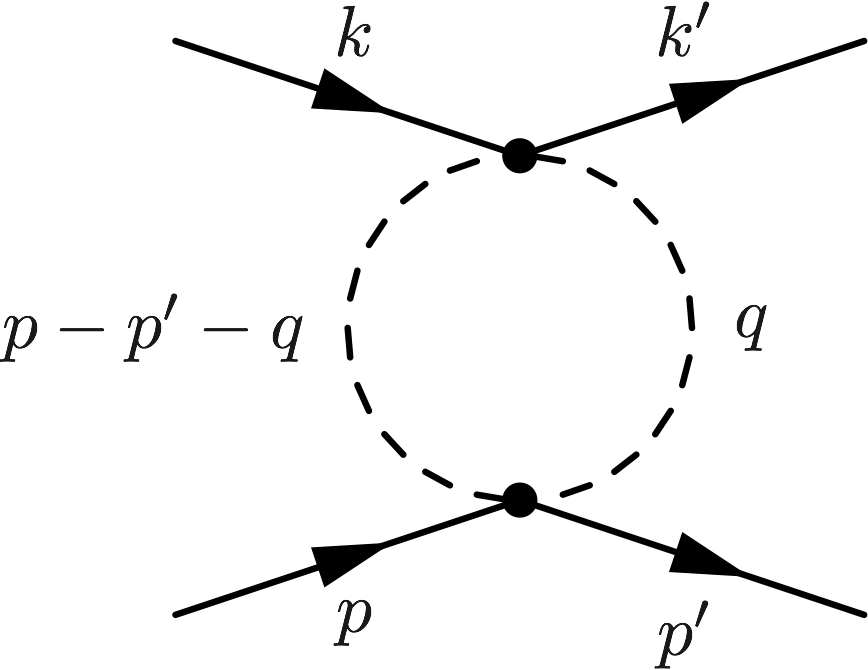
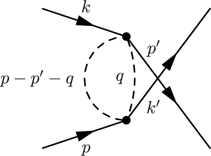
Figure 17: 1-loop Feynman diagrams that generates the non relativistic potential

Performing a contour integral to evaluate the integral over $|\textbf{q}|$ in the complex plane yields the potential between an electron and a heavy central body,

$$V\left(\mathbf{r}\right)=-\int\frac{d^{3}\mathbf{q}}{\left(2\pi\right)^{3}}G_{1-loop}\left(\mathbf{q}\right)e^{i\mathbf{q}\cdot\mathbf{x}}=\begin{cases}-\frac{(d^{(2)}_{m_{e}})^{2}Q^{C}_{m_{e}}m_{e}M_{C}}{(2M_{\rm Pl}^{2}\,)^{2}64\pi^{3}r^{2}}\frac{\sqrt{m_{\phi}}e^{-2m_{\phi}r}}{\sqrt{r}}&m_{\phi}r\gg 1\\ -\frac{(d^{(2)}_{m_{e}})^{2}Q^{C}_{m_{e}}m_{e}M_{C}}{(2M_{\rm Pl}^{2}\,)^{2}\,64\pi^{3}r^{3}}&m_{\phi}r\ll 1\,.\end{cases}$$ (C.6)

In the limit $m_{\phi}r\gg 1$, the potential is exponentially suppressed by $e^{-2m_{\phi}r}$ and $\frac{\sqrt{m_{\phi}}}{r^{5}/2}$, and thus negligible. We can also show that in the other limit i.e. $m_{\phi}r\ll 1$, the quantum potential is also negligible compare to the classical one. To see this, one can compare the accelerations from quantum and classical effects. The acceleration from quantum effect can be written as,

$$\lim_{m_{\phi}r\ll 1}\left|\Delta a^{\text{Quantum}}\right|\simeq\left|\frac{3(d^{(2)}_{m_{e}})^{2}Q^{C}_{m_{e}}M_{C}}{256\pi^{3}M_{\rm Pl}^{4}r^{4}}\right|\,.$$ (C.7)

Comparing Eq. (C.3) to Eq. (C.7) and using $\phi_{0}=\sqrt{2\rho_{\rm DM}}/m_{\phi}$ we find

$$\lim_{m_{\phi}r\ll 1}\left|\dfrac{\Delta a^{\text{Classical}}}{\Delta a^{\text{Quantum}}}\right| \simeq \frac{512\,\pi^{3}}{3\,d^{(2)}_{m_{e}}Q^{C}_{m_{e}}}\frac{\rho_{\text{DM}}M_{\rm Pl}^{2}\,}{m_{\phi}^{2}}\frac{R_{C}}{M_{C}}r^{2}\left[\frac{\Delta r}{R_{c}}\right]$$ (C.8)

$$\simeq 10^{50}\left[\frac{\Delta r}{R_{c}}\right]\left(\frac{10^{-14}\,\text{eV}}{m_{\phi}}\right)^{2}\left(\frac{\rho_{\rm DM}}{\rho_{\text{DM}}^{\odot}}\right)\,,$$

where, we take $r\simeq R_{C}$, and use the Earth as the source body with $Q^{C}_{m_{e}}\simeq 2.7\times 10^{-4}$. For the coupling, we use the current bound of $d^{(2)}_{m_{e}}\sim 10^{14}$ at the considered mass as shown in Fig. 2. Thus, even if one is very close to the surface of the central body (very close to the surface of the Earth), the classical effects are still dominating compare to the quantum ones. This is expected from the classical behavior of the scalar field, with a large occupation number.

Appendix D The Clockwork model

Consider $N+1$ complex scalar fields, $\Phi_{0}$ to $\Phi_{N}$, where each field represents a site on a lattice in the theory (field) space. The potential of these uncoupled sites is

$$V_{\text{clock}}\left(\left\{\Phi_{j}\right\}\right)=\sum_{i=0}^{N}\left(-m_{i}^{2}\Phi_{i}^{\dagger}\Phi_{i}+\lambda_{i}\left|\Phi_{i}^{\dagger}\Phi_{i}\right|^{2}\right)\,.$$ (D.1)

For simplicity, we consider the case where all couplings at different sites scale the same, i.e.

$$\forall_{i}:\;\;m_{i}^{2}\simeq m^{2}>0\,,\qquad\lambda_{i}\simeq\lambda\,.$$ (D.2)

Small deviation from the above alignment will have a negligible effect on the following analysis.

The clockwork potential has a $U\!\left(1\right)^{N+1}$ global symmetry which is broken spontaneously by $N+1$ VEVs of the complex scalar fields, $\left\langle\Phi_{i}\right\rangle\equiv\frac{f}{\sqrt{2}}=\sqrt{\frac{m^{2}}{2\lambda}}$. In addition to the above potential, we explicitly break the global $U\!\left(1\right)^{N+1}$ symmetry to a single $U\!\left(1\right)$, by connecting neighboring sites through a small parameter, $\left|\epsilon\right|<1$,

$$\Delta V_{\text{clock}}\left(\left\{\Phi_{j}\right\}\right)=-\sum_{j=0}^{N-1}\left(\epsilon\Phi_{j}^{\dagger}\Phi_{j+1}^{3}+\text{h.c.}\right)\,.$$ (D.3)

Expanding all the scalars around their VEVs,

$$\Phi_{j}=\frac{1}{\sqrt{2}}(f+\rho_{j})U_{j}\,,\qquad U_{j}=\text{e}^{i\pi_{j}/f}\,,$$

and taking the limit $\epsilon\ll\lambda\sim 1$, such that the radial modes can be decoupled, we get the following potential for the compact degrees of freedom,

$$\Delta V_{\text{clock}}\left(\left\{\pi_{j}\right\}\right)=-\frac{\epsilon f^{4}}{2}\sum_{j=0}^{N-1}\cos\left(\frac{3\pi_{j+1}-\pi_{j}}{f}\right)\,.$$

The above potential respects a $U\!\left(1\right)$ symmetry under which the fields, $\Phi_{0},\Phi_{1}...\Phi_{N}$, have charges $Q=1,\frac{1}{3}...,\frac{1}{3^{N}}$. The potential induces a mass matrix of the $N+1$ pNGBs,

$$M_{\left(\pi\right)}^{2}=\epsilon\frac{f^{2}}{2}\begin{pmatrix}1&-3&0&\cdots&&0\\ -3&10&-3&\cdots&&0\\ 0&-3&10&\cdots&&0\\ \vdots&\vdots&\vdots&\ddots&&\vdots\\ &&&&10&-3\\ 0&0&0&\cdots&-3&3^{2}\end{pmatrix}\,.$$

The matrix $M_{\left(\pi\right)}^{2}$ becomes diagonal in the field basis $\phi_{j}$ ($j=0,\,...,N$), related to the basis $\pi_{j}$ by a real $(N+1)\times(N+1)$ orthogonal matrix $O$,

$$\pi=O\phi\,,~{}~{}~{}~{}~{}~{}O^{T}M^{2}O={\rm diag}\left(m_{\phi_{0}}^{2},\dots,m_{\phi_{N}}^{2}\right)\,.$$

The eigenvalues of the mass matrix are given by

$$m_{\phi_{0}}^{2}=0\,,~{}~{}~{}m_{\phi_{k}}^{2}=\lambda_{k}\,\epsilon\frac{f^{2}}{2}\,,~{}~{}~{}~{}~{}k=1,..,N\,,$$ (D.4)

$$\lambda_{k}\equiv 10-6\cos\frac{k\pi}{N\!+\!1}\,.$$ (D.5)

The projection of the pNGB $\pi_{j}$, into the scalars in the mass basis $\phi_{k}$, are given by the elements of the rotation matrix,

$$O_{j0}=\frac{{\cal N}_{0}}{3^{j}}\,,~{}~{}~{}O_{jk}={\cal N}_{k}\left[3\sin\frac{jk\pi}{N\!+\!1}-\sin\frac{\left(j+1\right)k\pi}{N\!+\!1}\right]\,,~{}~{}~{}j=0,..,N\,;~{}~{}k=1,..,N$$

$${\cal N}_{0}\equiv\sqrt{\frac{9-1}{9-3^{-2N}}}\>,~{}~{}~{}~{}{\cal N}_{k}\equiv\sqrt{\frac{2}{(N\!+\!1)\lambda_{k}}}\>.$$ (D.6)

As expected by the breaking of $\left[U\left(1\right)\right]^{N+1}\rightarrow U\left(1\right)$ , there are $N$ massive scalars $\phi_{k},\;\left(k=1,...,N\right)$, and a single mass-less Goldstone whose wave function is exponentially peaked on the first site,

$$\phi\equiv\phi_{0}={\cal N}_{0}\sum_{j=0}^{N}\frac{1}{3^{j}}\pi_{j}\,.$$ (D.7)

For $N\gg 1$ the normalization constant is ${\cal N}_{0}(N)\approx\sqrt{8/9}$. The overlap between the mass-less eigenstate $\phi$ and the site $j$ is $\langle\pi_{j}|\phi\rangle\approx 1/3^{j}$. Under the spontaneously broken $U\!\left(1\right)_{\text{clock}}$ symmetry, $\phi$ and the other compact fields transform as follows,

$$U\!\left(1\right)_{\text{clock}}:\qquad \pi_{j}\mapsto\pi_{j}+\frac{1}{3^{j}}f\alpha\ ,$$

$$\phi\mapsto\phi+f\alpha\ ,$$ (D.8)

where $\alpha\in\left[0,2\pi\times 3^{N}\right]$. Introducing an explicit breaking of the global $U\!\left(1\right)_{\text{clock}}$ at the site $j$ would generate a potential for $\phi$ with periodicity of order $3^{j}f$. Therefore, by placing the backreaction sector at the $0^{\text{th}}$ site and the rolling sector at the $N^{\text{th}}$ site, we obtain the desired hierarchy between the periodicities, $F/f\approx 3^{N}$.

References

- (1) R. Catena and P. Ullio, A novel determination of the local dark matter density, JCAP 08 (2010) 004 [0907.0018].
- (2) P. W. Graham and S. Rajendran, New Observables for Direct Detection of Axion Dark Matter, Phys. Rev. D 88 (2013) 035023 [1306.6088].
- (3) A. Arvanitaki, J. Huang and K. Van Tilburg, Searching for dilaton dark matter with atomic clocks, Phys. Rev. D91 (2015) 015015 [1405.2925].
- (4) P. W. Graham, D. E. Kaplan, J. Mardon, S. Rajendran and W. A. Terrano, Dark Matter Direct Detection with Accelerometers, Phys. Rev. D93 (2016) 075029 [1512.06165].
- (5) A. Banerjee, H. Kim and G. Perez, Coherent relaxion dark matter, Phys. Rev. D100 (2019) 115026 [1810.01889].
- (6) E. W. Kolb and M. S. Turner, The Early Universe, vol. 69. 1990, 10.1201/9780429492860.
- (7) N. Bar, D. Blas, K. Blum and S. Sibiryakov, Galactic rotation curves versus ultralight dark matter: Implications of the soliton-host halo relation, Phys. Rev. D 98 (2018) 083027 [1805.00122].
- (8) N. Bar, K. Blum, J. Eby and R. Sato, Ultralight dark matter in disk galaxies, Phys. Rev. D 99 (2019) 103020 [1903.03402].
- (9) A. Arvanitaki, M. Baryakhtar and X. Huang, Discovering the QCD Axion with Black Holes and Gravitational Waves, Phys. Rev. D 91 (2015) 084011 [1411.2263].
- (10) M. Dine, The Problem of Axion Quality: A Low Energy Effective Action Perspective, 2207.01068.
- (11) A. Banerjee, J. Eby and G. Perez, From axion quality and naturalness problems to a high-quality ZN QCD relaxion, Phys. Rev. D 107 (2023) 115011 [2210.05690].
- (12) M. Kamionkowski and J. March-Russell, Planck scale physics and the Peccei-Quinn mechanism, Phys. Lett. B282 (1992) 137 [hep-th/9202003].
- (13) S. M. Barr and D. Seckel, Planck scale corrections to axion models, Phys. Rev. D46 (1992) 539.
- (14) O. Davidi, R. S. Gupta, G. Perez, D. Redigolo and A. Shalit, Nelson-Barr relaxion, Phys. Rev. D99 (2019) 035014 [1711.00858].
- (15) O. Davidi, R. S. Gupta, G. Perez, D. Redigolo and A. Shalit, The hierarchion, a relaxion addressing the Standard Model?s hierarchies, JHEP 08 (2018) 153 [1806.08791].
- (16) X. Calmet and F. Kuipers, Implications of quantum gravity for dark matter, Int. J. Mod. Phys. D 30 (2021) 2142004 [2107.13529].
- (17) G. Perez and A. Shalit, High quality Nelson-Barr solution to the strong CP problem with , JHEP 02 (2021) 118 [2010.02891].
- (18) K. Choi and J. E. Kim, DYNAMICAL AXION, Phys. Rev. D 32 (1985) 1828.
- (19) J. E. Kim, A COMPOSITE INVISIBLE AXION, Phys. Rev. D 31 (1985) 1733.
- (20) R. Contino, A. Podo and F. Revello, Chiral models of composite axions and accidental Peccei-Quinn symmetry, JHEP 04 (2022) 180 [2112.09635].
- (21) M. Dine, T. Banks and S. Sachdev, eds., Proceedings, Theoretical Advanced Study Institute in Elementary Particle Physics (TASI 2010). String Theory and Its Applications: From meV to the Planck Scale: Boulder, Colorado, USA, June 1-25, 2010, (Singapore), World Scientific, 2012. 10.1142/8153.
- (22) A. Hook, TASI Lectures on the Strong CP Problem and Axions, PoS TASI2018 (2019) 004 [1812.02669].
- (23) R. Oswald et al., Search for Dark-Matter-Induced Oscillations of Fundamental Constants Using Molecular Spectroscopy, Phys. Rev. Lett. 129 (2022) 031302 [2111.06883].
- (24) O. Tretiak, X. Zhang, N. L. Figueroa, D. Antypas, A. Brogna, A. Banerjee et al., Improved Bounds on Ultralight Scalar Dark Matter in the Radio-Frequency Range, Phys. Rev. Lett. 129 (2022) 031301 [2201.02042].
- (25) C. D. Froggatt and H. B. Nielsen, Hierarchy of Quark Masses, Cabibbo Angles and CP Violation, Nucl. Phys. B147 (1979) 277.
- (26) G. B. Gelmini and M. Roncadelli, Left-Handed Neutrino Mass Scale and Spontaneously Broken Lepton Number, Phys. Lett. B 99 (1981) 411.
- (27) J. E. Kim, Weak Interaction Singlet and Strong CP Invariance, Phys. Rev. Lett. 43 (1979) 103.
- (28) M. A. Shifman, A. I. Vainshtein and V. I. Zakharov, Can Confinement Ensure Natural CP Invariance of Strong Interactions?, Nucl. Phys. B 166 (1980) 493.
- (29) A. R. Zhitnitsky, On Possible Suppression of the Axion Hadron Interactions. (In Russian), Sov. J. Nucl. Phys. 31 (1980) 260.
- (30) M. Dine, W. Fischler and M. Srednicki, A Simple Solution to the Strong CP Problem with a Harmless Axion, Phys. Lett. B 104 (1981) 199.
- (31) P. W. Graham, D. E. Kaplan and S. Rajendran, Cosmological Relaxation of the Electroweak Scale, Phys. Rev. Lett. 115 (2015) 221801 [1504.07551].
- (32) Y. Ema, K. Hamaguchi, T. Moroi and K. Nakayama, Flaxion: a minimal extension to solve puzzles in the standard model, JHEP 01 (2017) 096 [1612.05492].
- (33) D. Brzeminski, Z. Chacko, A. Dev and A. Hook, Time-varying fine structure constant from naturally ultralight dark matter, Phys. Rev. D 104 (2021) 075019 [2012.02787].
- (34) T. Flacke, C. Frugiuele, E. Fuchs, R. S. Gupta and G. Perez, Phenomenology of relaxion-Higgs mixing, JHEP 06 (2017) 050 [1610.02025].
- (35) K. Choi and S. H. Im, Constraints on Relaxion Windows, JHEP 12 (2016) 093 [1610.00680].
- (36) A. Banerjee, H. Kim, O. Matsedonskyi, G. Perez and M. S. Safronova, Probing the Relaxed Relaxion at the Luminosity and Precision Frontiers, JHEP 07 (2020) 153 [2004.02899].
- (37) A. Hees, O. Minazzoli, E. Savalle, Y. V. Stadnik and P. Wolf, Violation of the equivalence principle from light scalar dark matter, Phys. Rev. D 98 (2018) 064051 [1807.04512].
- (38) T. Lin, Dark matter models and direct detection, PoS 333 (2019) 009 [1904.07915].
- (39) J. Alexander et al., Dark Sectors 2016 Workshop: Community Report, 8, 2016, 1608.08632.
- (40) A. Hook, Solving the Hierarchy Problem Discretely, Phys. Rev. Lett. 120 (2018) 261802 [1802.10093].
- (41) L. Di Luzio, B. Gavela, P. Quilez and A. Ringwald, An even lighter QCD axion, JHEP 05 (2021) 184 [2102.00012].
- (42) H. Kim and G. Perez, Oscillations of atomic energy levels induced by QCD axion dark matter, 2205.12988.
- (43) M. S. Safronova, D. Budker, D. DeMille, D. F. J. Kimball, A. Derevianko and C. W. Clark, Search for New Physics with Atoms and Molecules, Rev. Mod. Phys. 90 (2018) 025008 [1710.01833].
- (44) D. Antypas, D. Budker, V. V. Flambaum, M. G. Kozlov, G. Perez and J. Ye, Fast apparent oscillations of fundamental constants, Annalen Phys. 532 (2020) 1900566 [1912.01335].
- (45) E. Fischbach and C. Talmadge, Ten years of the fifth force, in 31st Rencontres de Moriond: Dark Matter and Cosmology, Quantum Measurements and Experimental Gravitation, pp. 443–451, 1996, hep-ph/9606249.
- (46) T. Damour and J. F. Donoghue, Equivalence Principle Violations and Couplings of a Light Dilaton, Phys. Rev. D 82 (2010) 084033 [1007.2792].
- (47) Y. V. Stadnik and V. V. Flambaum, Searching for dark matter and variation of fundamental constants with laser and maser interferometry, Phys. Rev. Lett. 114 (2015) 161301 [1412.7801].
- (48) Y. V. Stadnik and V. V. Flambaum, Can dark matter induce cosmological evolution of the fundamental constants of Nature?, Phys. Rev. Lett. 115 (2015) 201301 [1503.08540].
- (49) H. Masia-Roig et al., Intensity interferometry for ultralight bosonic dark matter detection, Phys. Rev. D 108 (2023) 015003 [2202.02645].
- (50) H. Banks and M. Mccullough, Charting the Fifth Force Landscape, Phys. Rev. D 103 (2021) 075018 [2009.12399].
- (51) R. Budnik, H. Kim, O. Matsedonskyi, G. Perez and Y. Soreq, Probing the relaxed relaxion and Higgs portal scenarios with XENON1T scintillation and ionization data, Phys. Rev. D 104 (2021) 015012 [2006.14568].
- (52) R. Balkin, J. Serra, K. Springmann, S. Stelzl and A. Weiler, Density induced vacuum instability, SciPost Phys. 14 (2023) 071 [2105.13354].
- (53) N. Bar, K. Blum and C. Sun, Galactic rotation curves versus ultralight dark matter: A systematic comparison with SPARC data, Phys. Rev. D 105 (2022) 083015 [2111.03070].
- (54) C. Dailey, C. Bradley, D. F. J. Kimball, I. A. Sulai, S. Pustelny, A. Wickenbrock et al., Quantum sensor networks as exotic field telescopes for multi-messenger astronomy, Nature Astronomy 5 (2020) 150.
- (55) H. Kim and A. Lenoci, Gravitational focusing of wave dark matter, Phys. Rev. D 105 (2022) 063032.
- (56) D. Budker, J. Eby, M. Gorghetto, M. Jiang and G. Perez, A Generic Formation Mechanism of Ultralight Dark Matter Solar Halos, 2306.12477.
- (57) A. Hook and J. Huang, Searches for other vacua. Part I. Bubbles in our universe, JHEP 08 (2019) 148 [1904.00020].
- (58) P. Salucci, F. Nesti, G. Gentile and C. Martins, The dark matter density at the Sun’s location, Astron. Astrophys. 523 (2010) A83 [1003.3101].
- (59) N. P. Pitjev and E. V. Pitjeva, Constraints on dark matter in the solar system, Astronomy Letters 39 (2013) 141.
- (60) Y.-D. Tsai, J. Eby, J. Arakawa, D. Farnocchia and M. S. Safronova, New Constraints on Dark Matter and Cosmic Neutrino Profiles through Gravity, 2210.03749.
- (61) S. Schlamminger, K. Y. Choi, T. A. Wagner, J. H. Gundlach and E. G. Adelberger, Test of the equivalence principle using a rotating torsion balance, Phys. Rev. Lett. 100 (2008) 041101 [0712.0607].
- (62) G. L. Smith, C. D. Hoyle, J. H. Gundlach, E. G. Adelberger, B. R. Heckel and H. E. Swanson, Short-range tests of the equivalence principle, Phys. Rev. D 61 (1999) 022001.
- (63) MICROSCOPE Collaboration collaboration, mission: Final results of the test of the equivalence principle, Phys. Rev. Lett. 129 (2022) 121102.
- (64) C. J. Kennedy, E. Oelker, J. M. Robinson, T. Bothwell, D. Kedar, W. R. Milner et al., Precision Metrology Meets Cosmology: Improved Constraints on Ultralight Dark Matter from Atom-Cavity Frequency Comparisons, Phys. Rev. Lett. 125 (2020) 201302 [2008.08773].
- (65) S. Aharony, N. Akerman, R. Ozeri, G. Perez, I. Savoray and R. Shaniv, Constraining Rapidly Oscillating Scalar Dark Matter Using Dynamic Decoupling, Phys. Rev. D 103 (2021) 075017 [1902.02788].
- (66) M. Abe, P. Adamson, M. Borcean, D. Bortoletto, K. Bridges, S. P. Carman et al., Matter-wave atomic gradiometer interferometric sensor (MAGIS-100), Quantum Science and Technology 6 (2021) 044003.
- (67) A. Hees, J. Guéna, M. Abgrall, S. Bize and P. Wolf, Searching for an oscillating massive scalar field as a dark matter candidate using atomic hyperfine frequency comparisons, Phys. Rev. Lett. 117 (2016) 061301 [1604.08514].
- (68) CAST collaboration, New CAST Limit on the Axion-Photon Interaction, Nature Phys. 13 (2017) 584 [1705.02290].
- (69) F. Capozzi and G. Raffelt, Axion and neutrino bounds improved with new calibrations of the tip of the red-giant branch using geometric distance determinations, Phys. Rev. D 102 083007 [2007.03694].
- (70) G. G. Raffelt, Astrophysical axion bounds, Lect. Notes Phys. 741 (2008) 51 [hep-ph/0611350].
- (71) M. Buschmann, C. Dessert, J. W. Foster, A. J. Long and B. R. Safdi, Upper Limit on the QCD Axion Mass from Isolated Neutron Star Cooling, Phys. Rev. Lett. 128 (2022) 091102 [2111.09892].
- (72) M. V. Beznogov, E. Rrapaj, D. Page and S. Reddy, Constraints on Axion-like Particles and Nucleon Pairing in Dense Matter from the Hot Neutron Star in HESS J1731-347, Phys. Rev. C 98 (2018) 035802 [1806.07991].
- (73) C. S. Reynolds, M. C. D. Marsh, H. R. Russell, A. C. Fabian, R. Smith, F. Tombesi et al., Astrophysical limits on very light axion-like particles from Chandra grating spectroscopy of NGC 1275, Astrophys. J. 890 (2020) 59 [1907.05475].
- (74) C. Abel et al., Search for Axionlike Dark Matter through Nuclear Spin Precession in Electric and Magnetic Fields, Phys. Rev. X 7 (2017) 041034 [1708.06367].
- (75) A. Banerjee, D. Budker, J. Eby, H. Kim and G. Perez, Relaxion Stars and their detection via Atomic Physics, Commun. Phys. 3 (2020) 1 [1902.08212].
- (76) A. Banerjee, D. Budker, J. Eby, V. V. Flambaum, H. Kim, O. Matsedonskyi et al., Searching for Earth/Solar Axion Halos, JHEP 09 (2020) 004 [1912.04295].
- (77) P. Touboul et al., MICROSCOPE Mission: First Results of a Space Test of the Equivalence Principle, Phys. Rev. Lett. 119 (2017) 231101 [1712.01176].
- (78) J. Bergé, P. Brax, G. Métris, M. Pernot-Borràs, P. Touboul and J.-P. Uzan, MICROSCOPE Mission: First Constraints on the Violation of the Weak Equivalence Principle by a Light Scalar Dilaton, Phys. Rev. Lett. 120 (2018) 141101 [1712.00483].
- (79) M. S. Safronova, The Search for Variation of Fundamental Constants with Clocks, Annalen Phys. 531 (2019) 1800364.
- (80) D. Antypas, O. Tretiak, K. Zhang, A. Garcon, G. Perez, M. G. Kozlov et al., Probing fast oscillating scalar dark matter with atoms and molecules, Quantum Sci. Technol. 6 (2021) 034001 [2012.01519].
- (81) T. A. Wagner, S. Schlamminger, J. H. Gundlach and E. G. Adelberger, Torsion-balance tests of the weak equivalence principle, Class. Quant. Grav. 29 (2012) 184002 [1207.2442].
- (82) Y. Su, B. R. Heckel, E. G. Adelberger, J. H. Gundlach, M. Harris, G. L. Smith et al., New tests of the universality of free fall, Phys. Rev. D 50 (1994) 3614.
- (83) A. Derevianko, K. Gibble, L. Hollberg, N. R. Newbury, C. Oates, M. S. Safronova et al., Fundamental physics with a state-of-the-art optical clock in space, Quantum Science and Technology 7 (2022) 044002.
- (84) A. Dymarsky, Z. Komargodski, A. Schwimmer and S. Theisen, On Scale and Conformal Invariance in Four Dimensions, JHEP 10 (2015) 171 [1309.2921].
- (85) F. Coradeschi, P. Lodone, D. Pappadopulo, R. Rattazzi and L. Vitale, A naturally light dilaton, JHEP 11 (2013) 057 [1306.4601].
- (86) T. R. Taylor and G. Veneziano, Dilaton Couplings at Large Distances, Phys. Lett. B 213 (1988) 450.
- (87) D. B. Kaplan and M. B. Wise, Couplings of a light dilaton and violations of the equivalence principle, JHEP 08 037 [hep-ph/0008116].
- (88) J. Lee, E. Adelberger, T. Cook, S. Fleischer and B. Heckel, New Test of the Gravitational Law at Separations down to 52 m, Phys. Rev. Lett. 124 (2020) 101101 [2002.11761].
- (89) W.-H. Tan et al., Improvement for Testing the Gravitational Inverse-Square Law at the Submillimeter Range, Phys. Rev. Lett. 124 (2020) 051301.
- (90) K. A. Olive and M. Pospelov, Environmental dependence of masses and coupling constants, Phys. Rev. D 77 (2008) 043524 [0709.3825].
- (91) E. Burt, J. Prestage, R. Tjoelker, D. Enzer, D. Kuang, D. Murphy et al., Demonstration of a trapped-ion atomic clock in space, Nature 595 (2021) 43.
- (92) T. A. Ely, E. A. Burt, J. D. Prestage, J. M. Seubert and R. L. Tjoelker, Using the deep space atomic clock for navigation and science, IEEE Transactions on Ultrasonics, Ferroelectrics, and Frequency Control 65 (2018) 950.
- (93) L. Liu, D.-S. Lü, W. biao Chen, T. Li, Q. Qu, B. Wang et al., In-orbit operation of an atomic clock based on laser-cooled 87rb atoms, Nature Communications 2760 (2018) .
- (94) L. Cacciapuoti, M. Armano, R. Much, O. Sy, A. Helm, M. P. Hess et al., Testing gravity with cold-atom clocks in space. The ACES mission, European Physical Journal D 74 (2020) 164.
- (95) A. D. Ludlow, M. M. Boyd, J. Ye, E. Peik and P. O. Schmidt, Optical atomic clocks, Reviews of Modern Physics 87 (2015) 637 [1407.3493].
- (96) S. M. Brewer, J.-S. Chen, A. M. Hankin, E. R. Clements, C. W. Chou, D. J. Wineland et al., quantum-logic clock with a systematic uncertainty below , Phys. Rev. Lett. 123 (2019) 033201.
- (97) J. Stuhler and other, Opticlock: Transportable and easy-to-operate optical single-ion clock, Measurement: Sensors 18 (2021) 100264.
- (98) D. Antypas et al., New horizons: Scalar and vector ultralight dark matter, arXiv: 2203.14915 (2022) .
- (99) Y.-D. Tsai, J. Eby and M. S. Safronova, Direct detection of ultralight dark matter bound to the Sun with space quantum sensors, Nature Astron. 7 (2023) 113 [2112.07674].
- (100) S. Kolkowitz, I. Pikovski, N. Langellier, M. Lukin, R. Walsworth and J. Ye, Gravitational wave detection with optical lattice atomic clocks, Physical Review D 94 (2016) .
- (101) M. A. Fedderke, P. W. Graham and S. Rajendran, Asteroids for Hz gravitational-wave detection, Phys. Rev. D 105 (2022) 103018 [2112.11431].
- (102) D. Puetzfeld and C. Lämmerzahl, eds., Relativistic Geodesy, vol. 196. Springer, 2019, 10.1007/978-3-030-11500-5.
- (103) D. R. Gozzard, L. A. Howard, B. P. Dix-Matthews, S. Karpathakis, C. Gravestock and S. W. Schediwy, Ultrastable Free-Space Laser Links for a Global Network of Optical Atomic Clocks, Phys. Rev. Lett. 128 (2022) 020801 [2103.12909].
- (104) I. Alonso et al., Cold atoms in space: community workshop summary and proposed road-map, EPJ Quant. Technol. 9 (2022) 30 [2201.07789].
- (105) V. Schkolnik et al., Optical atomic clock aboard an Earth-orbiting space station (OACESS): enhancing searches for physics beyond the standard model in space, Quantum Sci. Technol. 8 (2023) 014003 [2204.09611].
- (106) D. Hanneke, B. Kuzhan and A. Lunstad, Optical clocks based on molecular vibrations as probes of variation of the proton-to-electron mass ratio, Quantum Science and Technology 6 (2021) 014005 [2007.15750].
- (107) R. Allahverdi et al., The First Three Seconds: a Review of Possible Expansion Histories of the Early Universe, 2006.16182.
- (108) W. DeRocco, P. W. Graham and S. Rajendran, Exploring the robustness of stellar cooling constraints on light particles, Phys. Rev. D 102 (2020) 075015 [2006.15112].
- (109) G. Raffelt, Limits on a CP-violating scalar axion-nucleon interaction, Phys. Rev. D86 (2012) 015001 [1205.1776].
- (110) J. Redondo and G. Raffelt, Solar constraints on hidden photons re-visited, JCAP 1308 (2013) 034 [1305.2920].
- (111) E. Hardy and R. Lasenby, Stellar cooling bounds on new light particles: plasma mixing effects, JHEP 02 (2017) 033 [1611.05852].
- (112) K. Choi and S. H. Im, Realizing the relaxion from multiple axions and its UV completion with high scale supersymmetry, JHEP 01 (2016) 149 [1511.00132].
- (113) D. E. Kaplan and R. Rattazzi, Large field excursions and approximate discrete symmetries from a clockwork axion, Phys. Rev. D93 (2016) 085007 [1511.01827].