A limit on variations in the fine-structure constant from spectra of nearby Sun-like stars

The fine structure constant, $\alpha$, sets the strength of the electromagnetic force. The Standard Model of particle physics provides no explanation for its value, which could potentially vary. The wavelengths of stellar absorption lines depend on $\alpha$, but are subject to systematic effects owing to astrophysical processes in stellar atmospheres. We measured precise line wavelengths using 17 stars, selected to have almost identical atmospheric properties to those of the Sun (solar twins), which reduces those systematic effects. We found that $\alpha$ varies by  $<$$\sim$ 50 parts-per-billion (ppb) within 50 parsecs from Earth. Combining the results from all 17 stars provides an empirical, local reference for stellar measurements of $\alpha$ with an ensemble precision of 12 ppb.

The Standard Model of particle physics contains parameters known as “fundamental constants”. These include the coupling strengths of the known physical forces; the strength of electromagnetism is set by the fine-structure constant, $\alpha\equiv e^{2}/\hbar c$ where $e$ is the elementary charge, $\hbar$ is the reduced Planck constant and $c$ is the (vacuum) speed of light. These dimensionless numbers are referred to as “fundamental” because the Standard Model does not predict their values. They are usually assumed to be universal constants, i.e. they do not depend on other (unknown) physics. Their values can only be established experimentally, and testing their constancy requires measurements under a wide range of physical conditions, such as different times, distances, gravitational potentials etc.. Measurements of laboratory atomic clocks have set an upper limit on relative variations in $\alpha$ to $\,\hbox to0.0pt{\raise 1.50696pt\hbox{$<$}\hss}{\lower 3.01385pt\hbox{$\sim$}}\,10^{-18}$ yr^-1 over several years  (?). On cosmological time and distance scales, absorption lines of distant gas clouds in the spectra of background quasars limit relative variations in $\alpha$ to $\,\hbox to0.0pt{\raise 1.50696pt\hbox{$<$}\hss}{\lower 3.01385pt\hbox{$\sim$}}\,1$ parts per million (ppm)  (?, ?, ?). A study of giant stars within the Milky Way has set similar limits of $\,\hbox to0.0pt{\raise 1.50696pt\hbox{$<$}\hss}{\lower 3.01385pt\hbox{$\sim$}}\,2$–6 ppm  (?, ?).

Any variation in $\alpha$ would alter the energy levels of atoms and ions in characteristic ways  (?). The rest-frame wavenumber of an absorption or emission line, $\omega_{\rm obs}$, would shift from its laboratory value, $\omega_{0}$, in proportion to the relative change $\Delta\alpha/\alpha\equiv(\alpha_{\rm obs}-\alpha_{0})/\alpha_{0}$:

$$\frac{\Delta v}{c}\equiv\frac{\omega_{0}-\omega_{\rm obs}}{\omega_{0}}\approx-2\frac{\Delta\alpha}{\alpha}Q\,,$$ (1)

where $\alpha_{0}$ and $\alpha_{\rm obs}$ are the laboratory and observed values of $\alpha$, respectively, $\Delta v$ is the line shift in velocity units, and the sensitivity coefficient, $Q$, describes how much a given line shifts to the blue (for positive $Q$) or red. The approximation is valid for $\Delta\alpha/\alpha\ll 1$. In practice, the velocity shifts are measured for multiple lines and different atoms and ions, which is known as the Many Multiplet method. Utilising lines with a wide variety of $Q$ coefficients increases the sensitivity to variations in $\alpha$.

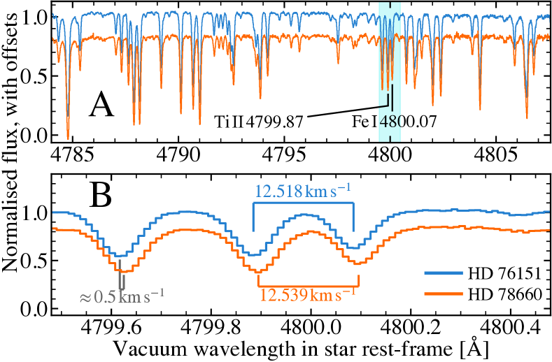
Figure 1: Example solar twin spectra. (A) Small sections of continuum-normalised HARPS spectra of two solar twins from our sample, HD 76151 (blue) and HD 78660 (orange), with the latter shifted down by 0.2 for clarity. Black labels indicate an example line pair used to constrain $\alpha$ variation. This is the least-separated pair of the 17 in our analysis; the maximum separation of 800 km s^-1 would span approximately half the width of this panel. The cyan shading indicates the region shown in panel B. (B) The measured velocity separations $\Delta v^{i}_{\rm raw}$, labelled in the figure, differ by 21 m s^-1, before correction for their stellar parameters (equation 2). In both panels, the spectra are shown in the stars’ rest frames; errors in their radial velocities are evident as a $\approx$0.5 km s^-1 shift between them (labelled in grey in panel B). Our differential approach is insensitive to that offset.

Sun-like stars are a potentially suitable target for the Many Multiplet method: their spectra contain thousands of narrow, well-defined, strong (but unsaturated) absorption lines (Fig. 1A). The observed wavelengths of these lines could, in principle, be compared to their laboratory values while simultaneously accounting for the star’s radial velocity. However, this simple approach is limited by large systematic errors: several physical mechanisms can shift the lines by up to $\sim$700 m s^-1 from their laboratory wavelengths, and the line profiles are asymmetric because they arise over a range of depths in stellar atmospheres  (?, ?). These effects produce velocity shifts between lines, typically $\Delta v\sim 250$ m s^-1  (?), which is equivalent to $\Delta\alpha/\alpha\sim 6$ ppm for a typical range in $Q$ coefficients of $\approx$0.07  (?). Direct comparison of absorption lines in a single giant star to laboratory values has already reached this systematic error limit  (?).

We adopt an alternative technique that compares absorption lines between stars that have intrinsically similar spectra, thereby eliminating the need to compare with laboratory wavelengths. The atmospheric spectrum of an isolated main-sequence star depends primarily on its mass and heavy-element content, which determine three primary observable parameters: the effective temperature $T_{\rm eff}$, iron metallicity [Fe/H], and surface gravity $\log g$. We restrict our analysis to solar twins – defined as stars with these parameters within 100 K, 0.1 dex and 0.2 dex of the Sun’s values, respectively. Spectra of two solar twins used in our analysis are shown in Fig. 1A. We measure the velocity-space separations of pairs of lines, then compare the same sets of lines between stars (Fig. 1B). This approach reduces the systematic errors from astrophysical line shifts and asymmetries because of the similarity of their stellar parameters. The use of pairs of lines removes any dependence on the stars’ radial velocities, including any variations that could be caused by an orbiting companion (e.g. in a planetary or binary stellar system). For main-sequence stars, line shifts and asymmetries are observed to be correlated with the line’s optical depth and wavelength  (?), so we select pairs with similar absorption depths (within 20%) and small separations ($<$800 km s^-1, equivalent to $\approx$13 Å at 5000 Å)  (?, ?, ?). We chose these values to reduce the systematic effects while maintaining sensitivity to variations in $\alpha$ between stars.

We applied this solar twins method to archival solar twin spectra from the High Accuracy Radial velocity Planet Searcher (HARPS) spectrograph mounted on the European Southern Observatory (ESO) 3.6 m telescope at La Silla Observatory, Chile. HARPS is highly stable over time  (?) and its wavelength scale has been precisely characterised by using laser frequency combs  (?, ?). This sets an instrumental systematic error limit of $\sim$2–3 m s^-1 in the velocity separations of line pairs  (?). To reach this level we restricted our analysis to HARPS exposures corrected for non-uniform detector pixel sizes (corrections $\sim$25 m s^-1)  (?, ?), and applied a further correction for sparsely-sampled wavelength calibration (corrections $\sim$5 m s^-1)  (?, ?).

We selected 16 bright (i.e. nearby) solar twins with HARPS spectra, with signal-to-noise $\textrm{SNR}>200$ per 0.8 km s^-1 pixel, plus the Sun via its reflection from the asteroid Vesta (with $\textrm{SNR}>150$) (Table S1)  (?). With these SNRs, the statistical uncertainty in the velocity separation of two unresolved absorption lines is $\sim$25 m s^-1 from a single exposure, assuming that they absorb 50% of the stellar flux at their cores  (?). The median number of HARPS exposures available was 10 exposures per star (range of 1–138), so by combining results from multiple exposures we expect median statistical uncertainties to reduce to $\sim$8 m s^-1 per line pair, per star. By averaging over the sample of 17 stars, the uncertainty approaches that imposed by the available instrument calibration  (?).

From 8843 lines listed in a solar atlas  (?), we select 22 that are separated from each other and not blended with other nearby stellar or telluric (Earth atmosphere) lines  (?, ?). All 22 are strong but unsaturated, absorbing 15–90% of the continuum in the HARPS spectrum of the Sun. The 22 lines, which form 17 different pairs (some of which share common lines), arise from neutral atoms Na, Ca, Ti, V, Cr, Fe and Ni, plus singly-ionised Ti. Their $Q$ coefficients have been calculated previously  (?). The 17 pairs of lines have a wide range of sensitivity to $\alpha$ variation, with differences in $Q$ within each pair from $-0.08$ to $+0.18$  (?).

Pair separations were measured using a fully automated process for all of the 423 HARPS exposures. In each exposure, the core of each line – the central 7 pixels, spanning $\approx$5.7  km s^-1 – was fitted with a Gaussian model to determine the centroid wavelength. The wavelength differences between line pairs in each exposure were then computed, incorporating the corrections for the effects discussed above  (?, ?, ?). We denote these pair separations $\Delta v^{i}_{\rm raw}$ for pair $i$. In principle, they can be compared to gauge any $\alpha$ variation between these 17 solar twins. However, an analysis of 130 stars spanning a larger range in $T_{\rm eff}$, [Fe/H] and $\log g$ (300 K, 0.3 dex and 0.4 dex around solar values, respectively), has shown that pair velocity separation varies systematically with the stellar parameters, typically by $\sim$60 m s^-1 across this range  (?, ?). We fit a quadratic model to those correlations and use it to compute the expected line pair separation for each star in our sample, denoting the resulting values $\Delta v^{i}_{\rm model}$. We also incorporate an intrinsic star-to-star scatter, $\sigma^{i}_{**}\approx 0$ to 15 m s^-1  (?, ?). We then use $\Delta v^{i}_{\rm model}$ to correct the observed separations for each individual star:

$$\Delta v^{i}_{\rm sep}=\Delta v^{i}_{\rm raw}-\Delta v^{i}_{\rm model}(T_{\rm eff},{\rm[Fe/H]},\log g)\,.$$ (2)

For each line pair $i$, the value of $\sigma^{i}_{**}$ is the systematic error in $\Delta v^{i}_{\rm sep}$; it is the typical absolute value of the intrinsic deviation from the model.

The $\Delta v^{i}_{\rm sep}$ values have previously been calculated  (?) from the HARPS solar twin exposures. For each line pair in each solar twin, the velocity separation measurements from multiple exposures were combined using a weighted mean, with outliers excluded via an iterative process  (?, ?). Multiple exposures were available for 14 of the solar twins, allowing us to check for systematic errors as a function of time. The optical fibres that feed light from the telescope into HARPS were changed in mid-2015, resulting in large calibration changes. Analysis of the pre- and post-fibre change epochs separately – including the determination of $\Delta v^{i}_{\rm model}$ – has shown no evidence for systematic differences in $\Delta v^{i}_{\rm sep}$ between them  (?). We therefore combined their weighted mean $\Delta v^{i}_{\rm sep}$ values. Three of the 17 line pairs appear twice in each exposure, because they are in the overlapping wavelength ranges of neighbouring diffraction orders. We treat these two instances separately because we found differences of $\sim$20 m s^-1 between their $\Delta v^{i}_{\rm raw}$ values, which we ascribe to optical distortions within HARPS. Nevertheless, their weighted mean $\Delta v^{i}_{\rm sep}$ values show no systematic differences for our 17 stars, or the larger sample  (?), so we combine the $\Delta v^{i}_{\rm sep}$ value for two instances of a pair using a weighted mean.

Figure 2 shows our derived values of $\Delta\alpha/\alpha$ for each star. The $\Delta v^{i}_{\rm sep}$ value for a line pair $i$ is converted to $\Delta\alpha/\alpha$ using equations 1 and 2, and the $Q$ coefficient calculations  (?). For each star plotted (Fig. 2), the $\Delta\alpha/\alpha$ values from all pairs are consistent with each other, so they are combined using a weighted mean. The weights in that process, and the final uncertainties plotted (Fig. 2), include the statistical uncertainties, derived from the SNR of the HARPS spectra, and systematic errors that incorporate the star-to-star scatters for all line pairs ($\sigma^{i}_{**}$) and a smaller contribution from the uncertainties in the $Q$ coefficients. Because a line can be shared by multiple pairs, its statistical and systematic uncertainties cause correlated errors across those pairs; we used a Monte Carlo method to compute the combined $\Delta\alpha/\alpha$ value and its statistical and systematic uncertainty for each star  (?).

We find no variations in $\alpha$ between nearby solar twins ($<$50 parsec), with a typical (median) uncertainty in $\Delta\alpha/\alpha$ of $\approx$50 parts per billion (ppb; adding statistical and systematic errors in quadrature). The precision reaches $\approx$30 ppb for some stars, which is  $>$$\sim$ 30 times more precise than individual quasar absorption systems  (?, ?). The systematic error term dominates in these cases (Fig. 2), mainly due to the intrinsic star-to-star scatter, $\sigma^{i}_{**}\approx 0$ to 15 m s^-1 per line pair $i$. That is, the solar twins method allows  $>$$\sim$ 100 times more accuracy than comparison between lines in individual white dwarfs or giant stars with their laboratory counterparts  (?, ?). The results for the 17 stars are formally consistent with each other, with $\chi^{2}=18.2$ around their weighted mean (16 degrees of freedom; 31% probability of a larger value by chance alone), so there is no evidence for additional systematic errors that are not accounted for by $\sigma^{i}_{**}$.

Another study  (?) considered a variety of astrophysical and instrumental effects that could cause spurious variation of $\alpha$ between stars and/or account for $\sigma^{i}_{**}$. Apart from those already corrected in our analysis (e.g. wavelength calibration distortions), that study ruled out systematic error contributions from line blending, pair separation, differences in line depth in a pair, transiting exoplanets or magnetic activity cycles of the target stars, contamination of spectra by scattered moonlight, cosmic ray events or charge transfer inefficiencies in the detector. However, they estimated that variations in stellar rotation velocities or elemental and isotopic abundances between stars may plausibly explain the size of, and variations in, $\sigma^{i}_{**}$  (?). Nevertheless, they did not find specific evidence for these effects with simple tests, even amongst the larger data sample of stars used  (?).

Combining the results from all 17 stars provides a weighted mean with 12 ppb ensemble precision:

$$\left<\Delta\alpha/\alpha\right>_{\rm w}=7\pm 5_{\rm stat}\pm 11_{\rm sys}\,{\rm ppb}\,,$$ (3)

where $\left<\Delta\alpha/\alpha\right>_{\rm w}$ and its 1$\sigma$ statistical uncertainty and systematic error were calculated from the Monte Carlo simulations to account for the correlations between results for different stars because they share common line pairs  (?). The weights are the inverse variances from quadrature addition of the statistical and systematic uncertainties in $\Delta\alpha/\alpha$ for each star. The combined result (equation 3) acts as an entirely empirical reference for stellar measurements of $\alpha$. This, and the ability of our automatic analysis procedure to recover shifts in $\alpha$ between stars, was tested by altering the wavelength measurements for half our twins by amounts corresponding to an $\alpha$ variation of 100 ppb  (?). Re-running the full analysis but removing these stars from the determination of $\Delta v^{i}_{\rm model}$, we recovered an $86\pm 19$ ppb difference between the shifted and unshifted twins. The discrepancy arises because some measurements of shifted lines are excluded as outliers – the shifts introduced are much larger than the total uncertainties (including $\sigma^{i}_{**}$). This confirms that our analysis process would still have detected any large ($\sim$100 ppb) discrepancies between some twins if they were present in the data.

Supplementary Materials

Materials and Methods
Figs. S1 to S4
Tables S1 to S3
References (23–34)

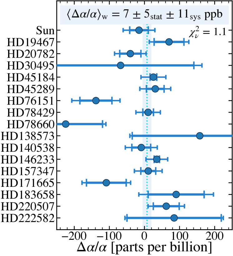
Figure 2: Fine-structure constant measurements. The relative deviation of the fine-structure constant, $\Delta\alpha/\alpha$, is shown for each star in our sample. These values are averages of all 17 line pairs for each star. The inner large error bars indicate the 1$\sigma$ statistical uncertainties, dominated by the number of observations available of each star, while the outer small error bars combine the statistical and systematic uncertainties in quadrature. The weighted mean of the sample, $\left<\Delta\alpha/\alpha\right>_{\rm w}$, is shown as the dotted cyan line; the blue shaded region shows the combined 1$\sigma$ statistical and systematic uncertainties. $\chi^{2}_{\nu}=1.1$ is the reduced $\chi^{2}$ (per degree of freedom) of the individual measurements around the weighted mean.

Supplementary Materials for

Strong limit on variations in the fine-structure constant from spectra of nearby Sun-like stars

Michael T. Murphy,^∗ Daniel A. Berke, Fan Liu (刘凡), Chris Flynn,
Christian Lehmann, Vladimir A. Dzuba, Victor V. Flambaum

This PDF file includes:
Materials and Methods
Figs. S1 to S4
Tables S1 to S3

Materials and Methods

The full details of the solar twins analysis are presented elsewhere  (?), as is an application to a larger sample of solar analogues (broader than solar twins)  (?). We adopt their modelling of raw line pair separations as functions of the main stellar atmospheric parameters: effective temperature $T_{\rm eff}$, iron metallicity [Fe/H], and surface gravity $\log g$  (?). Here we summarise that analysis, and provide further details about the conversion of the pair velocity separations to $\Delta\alpha/\alpha$.

Spectral line selection

An initial catalogue of 8843 lines in the Sun’s spectrum was drawn from the Belgian Repository of fundamental Atomic data and Stellar Spectra (BRASS)  (?). Most lines (90%) were excluded because they fell within 100 km s^-1 of telluric lines or within 3.5 HARPS resolution elements (9.1 km s^-1) of another stellar line. The former tolerance represents the maximum velocity shift possible for lines in our sample of stars, which have radial velocities of $\pm$70 km s^-1, given the Earth’s annual barycentric velocity variation of $\pm$30 km s^-1. All telluric lines that absorb $\geq$0.1% of the continuum were avoided to ensure that the fitted centroid of any individual stellar line of interest was affected by, at most, $\approx$30 m s^-1 in a single observation. Of the remaining 849 lines, 7% were removed because they were very weak or near saturation ($<$15% or $>$90% absorption depth, respectively) as measured in a HARPS spectrum of Vesta  (?). Most of the remaining 783 lines (79%) were then excluded because they appeared to be blended with other stellar lines at HARPS’s resolving power ($R\approx 115,000$)  (?). Only close pairs of lines (within 800 km s^-1), which had similar absorption depths (within 20%), were then selected. This left 164 lines, contributing to 229 pairs for study  (?). We adopted calculated sensitivity coefficients, $q$ (?), for 22 of these lines, where $Q\equiv q/\omega_{0}$, with $\omega_{0}$ the rest-frame wavenumber (see equation 1). These 22 lines, which we combine to form 17 pairs (some pairs share common lines), constitute the spectral line sample for which pair velocity separations were measured  (?). We calculate their $\Delta\alpha/\alpha$ values below.

Stellar sample and spectroscopic data selection

Beyond the requirement that stars in our sample must have been observed with HARPS, our main goal in selecting a stellar sample was to reduce bias in our study of solar twins. Our method requires a model of the variation of line pair separations with stellar parameters. It is therefore desirable for the sample to uniformly sample the three-dimensional stellar parameter space to avoid biases. For example, if the sample was concentrated on the solar twins range, with sparser sampling outside it, the models of variations in pair separation would have been unduly weighted towards the twins. Therefore we selected the sample from an approximately homogenous starting catalogue  (?).

We selected stars from the 14139 F and G dwarfs in the Geneva–Copenhagen Survey  (?). Using improved photometric stellar parameter estimates  (?), this catalogue contains 711 ‘solar type’ stars according to a standard definition  (?), 200 of which had at least one exposure with signal-to-noise ratio $200\leq{\rm SNR}\leq 400$ per 0.8 km s^-1 HARPS pixel in the ESO archive  (?). To this sample we added the Sun, observed indirectly via reflection from the asteroid Vesta; to increase the number of Vesta exposures used in our analysis, we only required a threshold SNR of 150 per pixel. Of these 201 stars, 136 had exposures for which corrections to the wavelength calibration for non-uniform detector pixel sizes were available  (?). Finally, to reduce the number of lines falling near telluric features, we removed 6 stars with absolute radial velocities $>$70 km s^-1 (see above).

These 130 ‘solar type’ stars were used to model the variation of each line pair’s velocity separation with stellar atmospheric parameters  (?, ?). These parameters differ from the solar values  (?) (i.e. $T_{\rm eff}=5772$ K, $\textrm{[Fe/H]}=0.0$ dex, $\log g=4.44$ dex, for $g$ in units of cm s^-1) over the following ranges: $-350\leq\Delta T_{\rm eff}\leq 450$ K, $-0.65\leq\textrm{[Fe/H]}\leq 0.40$ dex and $-0.3\leq\log g\leq 0.2$. The pair velocity separations have been measured for the 18 ‘solar twins’ in this sample  (?), i.e. where the stellar parameters differed by 100 K, 0.1 dex and 0.2 dex from the solar values, respectively. We exclude the results from one of these stars (HD 1835) because the single HARPS exposure available provided much weaker constraints on $\Delta\alpha/\alpha$ than the other stars ($\Delta\alpha/\alpha\approx 2300$ ppb with total uncertainty  $>$$\sim$ 1200 ppb). Table S1 provides the ESO Programme identification codes for the HARPS exposures of the 17 stars studied here.

Table S1: Origin of the HARPS exposures. The first column provides the ESO Programme identification codes, with the principal investigator named in the second column. The third column provides the names of the objects observed.

Project ID	PI Name	Objects
60.A-9036	ESOa	HD 45184, HD 183658, Vesta
072.C-0488	M. Mayor	HD 19467, HD 20782, HD 45184, HD 45289, HD 76151,
		HD 78429, HD 146233, HD 157347, HD 171665, HD 183658,
		HD 220507, HD 222582
075.C-0332	C. H. F. Melo	HD 78660, HD 140538
077.C-0364	M. Mayor	HD 146233, HD 171665, HD 183658
088.C-0323	A. Cameron	Vesta
091.C-0936	S. Udry	HD 45184
183.C-0972	S. Udry	HD 19467, HD 20782, HD 45184, HD 45289, HD 76151,
		HD 146233, HD 157347, HD 171665, HD 183658, HD 220507,
		HD 222582
183.D-0729	M. Bazot	HD 78660, HD 146233, HD 220507
188.C-0265	J. Meléndez	HD 19467, HD 30495, HD 45289, HD 78660, HD 138573,
		HD 140538, HD 146233, HD 157347, HD 183658, HD 220507
192.C-0852	S. Udry	HD 19467, HD 20782, HD 45184, HD 78429, HD 146233,
		HD 157347, HD 183658, HD 220507, HD 222582
196.C-1006	S. Udry	HD 20782, HD 78429, HD 146233, HD 220507
198.C-0836	R. Diaz	HD 45184, HD 78429, HD 146233, HD 220507

^aESO uses the project ID 60.A-9036 to indicate observations undertaken for calibration or engineering purposes.

Data processing and line wavelength measurement

The HARPS spectra were processed automatically by the HARPS Data Reduction System (DRS)  (?). We used intermediate data products to produce a flux uncertainty array for each echelle order, following the approach of a previous study  (?), to determine an uncertainty estimate for the centroid wavelength of each spectral feature. The flux and uncertainty arrays are not merged to form a one dimensional spectrum. Instead, the observed wavelength of each line is measured from the two dimensional spectrum of the one or two echelle orders in which it falls.

Line positions were determined by fitting a Gaussian model to the central 7 pixels, equivalent to the central $\approx$5.7  km s^-1 of the line, which reduces line asymmetry effects  (?, ?). For each pixel, the Gaussian profile is averaged, rather than evaluated only at its centre, to account for the non-uniform flux distribution across its spectral dimension  (?). The resulting centroid wavelength is already corrected (by the DRS) for the barycentric motion of the Earth during the observation and the non-uniform detector pixel sizes. An additional wavelength correction is applied to account for inaccuracies in the standard thorium–argon lamp wavelength calibration  (?): a low-order polynomial model fitted to a small number of calibration lines on each echelle order leaves $\sim$5 m s^-1 distortions in the calibration, even after correction for the non-uniform pixel sizes  (?).

Before the observed line wavelengths from a single exposure are used to measure pair separations, their offsets from their respective laboratory wavelengths are used for identifying if any of them are outliers. This allows the rejection of lines in which a cosmic ray event affected the flux recorded in one or more of the seven fitted pixels. The offset for a single line is strongly correlated with the primary three stellar parameters, $T_{\rm eff}$, [Fe/H] and $\log g$, so it was modelled as a quadratic function in each of these parameters  (?, ?). As an example, Fig. S1 shows the variation in the offset for one line, Fe i 6138.313, as a function of metallicity. The line offset measurements and models for all stars are provided elsewhere  (?, ?). For each exposure of each star, individual lines whose offsets deviated from the model by more than 3 times their statistical uncertainties were rejected. This was determined in an iterative procedure in which the best-fitting radial velocity for the exposure was simultaneously measured. This procedure employed all 164 lines that satisfied the line selection criteria discussed above.

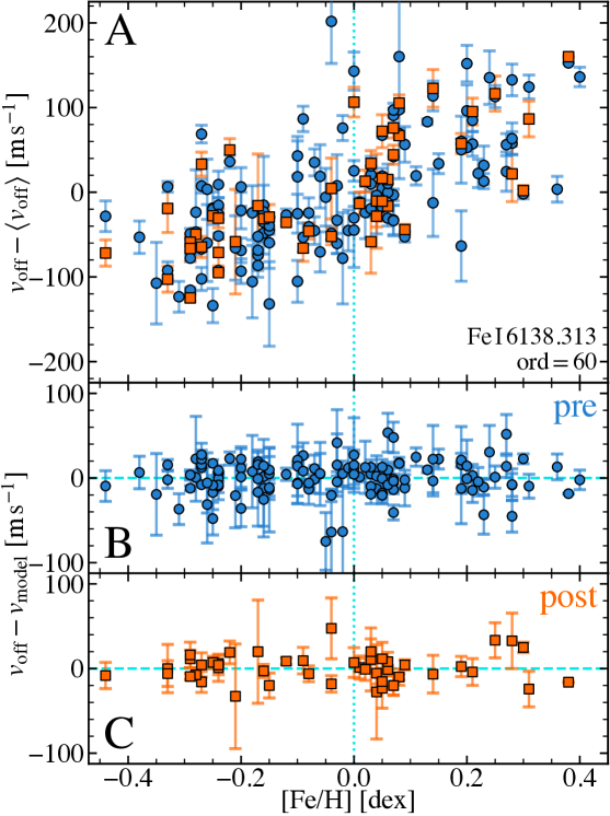
Figure S1: Example of variation in line offset with metallicity, [Fe/H]. (A) Deviation of the measured line offset from its laboratory wavelength, $\Delta v_{\rm off}$, from the mean value, $\left<\Delta v_{\rm off}\right>$, in 130 ‘solar type’ stars  (?) for the line Fe i 6138.313 in echelle order 60. Blue circles and orange squares indicate measurements from spectra observed in the pre- and post-fibre change epochs, respectively. Error bars indicate the 1$\sigma$ statistical uncertainties derived from the signal-to-noise ratio of the spectra. (B) Differences between the $v_{\rm off}$ values and the quadratic model, $v_{\rm model}$, calculated for the pre-fibre change measurements in panel A  (?, ?). The dashed horizontal cyan line indicates zero deviation from the model. (C) Same as for panel B but for the post-fibre change measurements. The dotted vertical cyan line in all panels indicates the solar metallicity. Stars for which all measurements of this line were rejected as outliers appear in panel A but not in the lower two panels.

Pair separation models

Convective motions in stellar atmospheres shift and skew the shapes of stellar lines  (?, ?). More photons are emitted from hotter, up-welling convective cells (granules) than colder, sinking ones, which shifts stellar lines bluewards from laboratory wavelengths. The blueshift varies with depth in the photosphere, as do the local conditions (temperature and pressure) which affect the line-width. Each observed stellar line is the cumulative result of differing amounts of absorption over a range of depths, so the line profile is asymmetric, with the degree of asymmetry varying as a function of the line’s absorption depth (i.e. the line bisector is not at a constant offset from the laboratory wavelength). The shift and asymmetry differs for each line because the amount of absorption, at a given depth in the photosphere, depends on the atomic physics of that line, e.g. the ionisation level, the line’s initial energy state and quantum mechanical probability. Our solar twins approach attempts to reduce these effects by comparing the separations between the same pair of lines in very similar stars. The astrophysical shifts and asymmetries will also depend on the physical conditions in the photosphere, characterised by the stellar atmospheric parameters $T_{\rm eff}$, [Fe/H] and $\log g$.

We therefore expect variations in the observed separation between pairs of stellar lines as functions of these parameters. These are likely to be of a similar magnitude, though somewhat smaller than, the astrophysical shifts and asymmetries themselves, which are observed to be up to $\sim$700 m s^-1 in individual lines  (?, ?). The larger, ‘solar type’ sample of 130 stars  (?) showed that the raw pair separation – $\Delta v^{i}_{\rm raw}$ in equation (2) – varies with the stellar parameters. As an example, one line pair has a separation which varies by $\sim$400 m s^-1 over the metallicity range $-0.4<\textrm{[Fe/H]}<0.4$ dex [ (?), their figure 15]. While this was noted as larger than typical, it was not unrepresentative. For the 17 pairs studied in this paper, the variation is $\sim$150 m s^-1 at most. Fig. S2A shows an example where the variation is $\sim$100 m s^-1 over the same metallicity range, and Fig. S3 shows the variation for each pair as a function of all three stellar parameters ($T_{\rm eff}$, [Fe/H] and $\log g$).

The variation in pair separation was found to be a low-order, generally monotonic function of the stellar parameters for almost all the 229 pairs included in the previous study  (?), including all of the 17 pairs used in this paper. This implies that we can use an empirical model for $\Delta v^{i}_{\rm model}$ in equation (2), for each pair $i$, to provide a local reference for the pair separation for any solar analogue star. We found that a quadratic model adequately tracked the variation of $\Delta v^{i}_{\rm raw}$ with $T_{\rm eff}$, [Fe/H] and $\log g$. Incorporating this model allows us to compare stars which are not perfect twins of each other, having different stellar parameters.

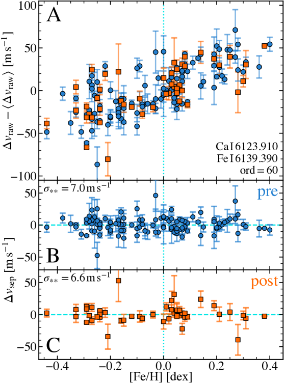
Figure S2: Example of variation in line pair separation with metallicity, [Fe/H]. (A) Deviation of the measured pair separations, $\Delta v_{\rm raw}$, from their mean value, $\left<\Delta v_{\rm raw}\right>$, in 130 ‘solar type’ stars  (?) for the line pair and echelle order labelled in the figure: Ca i 6123.910 and Fe i 6139.390 in order 60. Blue circles and orange squares indicate measurements from spectra observed in the pre- and post-fibre change epochs, respectively. Error bars indicate the 1$\sigma$ statistical uncertainties derived from the signal-to-noise ratio of the spectra. (B) Values of $\Delta v_{\rm sep}$ calculated for the pre-fibre change measurements in panel A, i.e. the deviation of $\Delta v_{\rm raw}$ from the quadratic model of its variation with all three stellar parameters, $T_{\rm eff}$, [Fe/H] and $\log g$ (equation 2). The star-to-star scatter, $\sigma_{**}$ labelled in the figure, measures the additional scatter of $\Delta v_{\rm sep}$ in excess of that expected from the statistical uncertainties. The dashed horizontal cyan line indicates zero deviation from the model. (C) Same as for panel B but for the post-fibre change measurements. The dotted vertical cyan line in all panels indicates the solar metallicity.

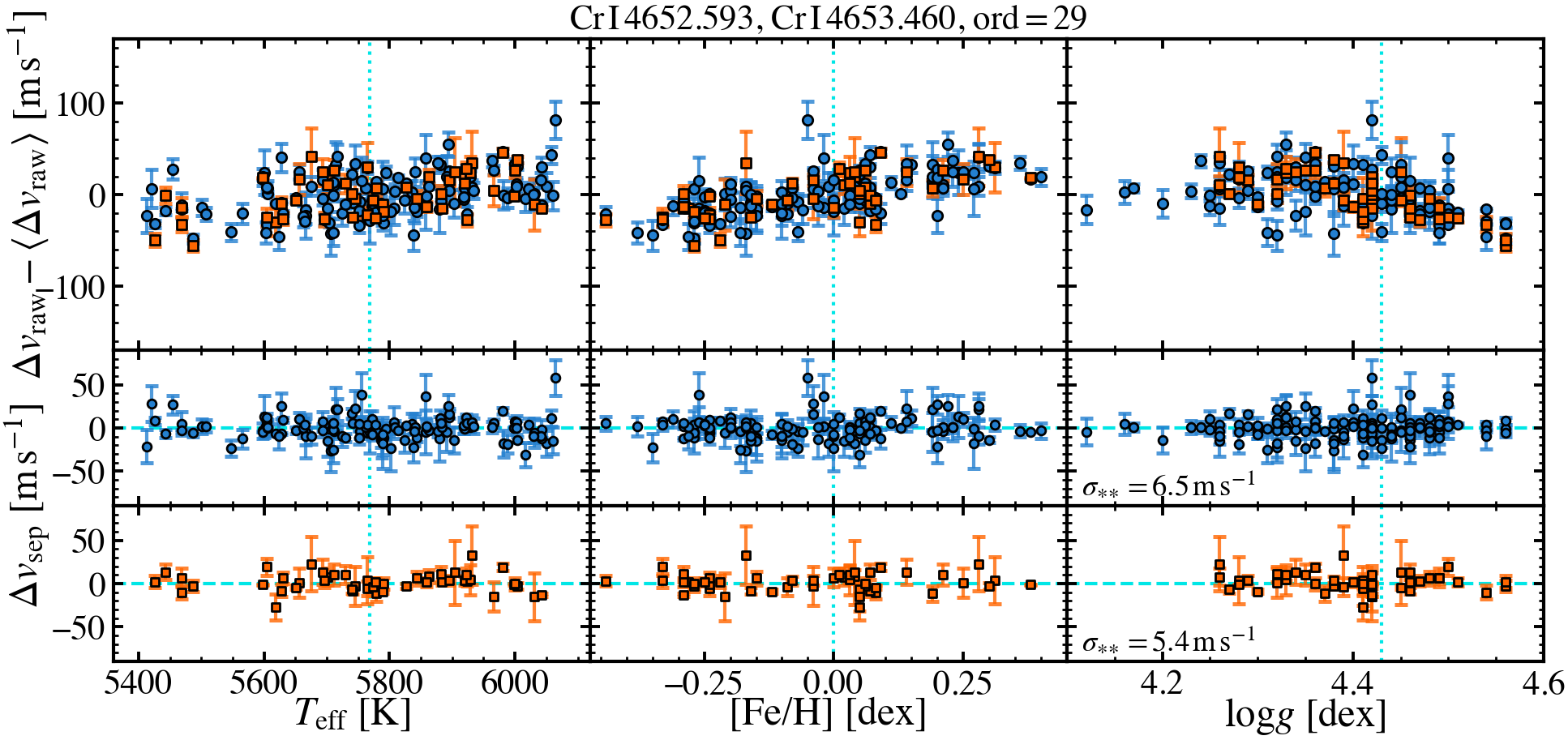
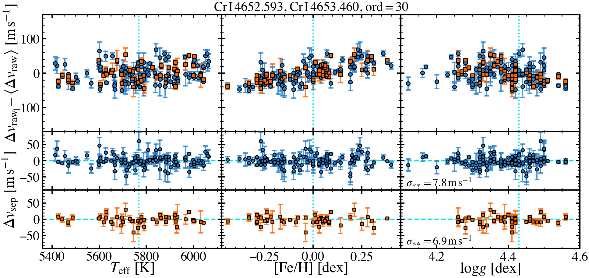
Figure S3: Variation in line pair separations. Same as for Fig. S2 but for all three stellar parameters ($T_{\rm eff}$, [Fe/H] and $\log g$) and the pairs and echelle orders labelled above the figures.

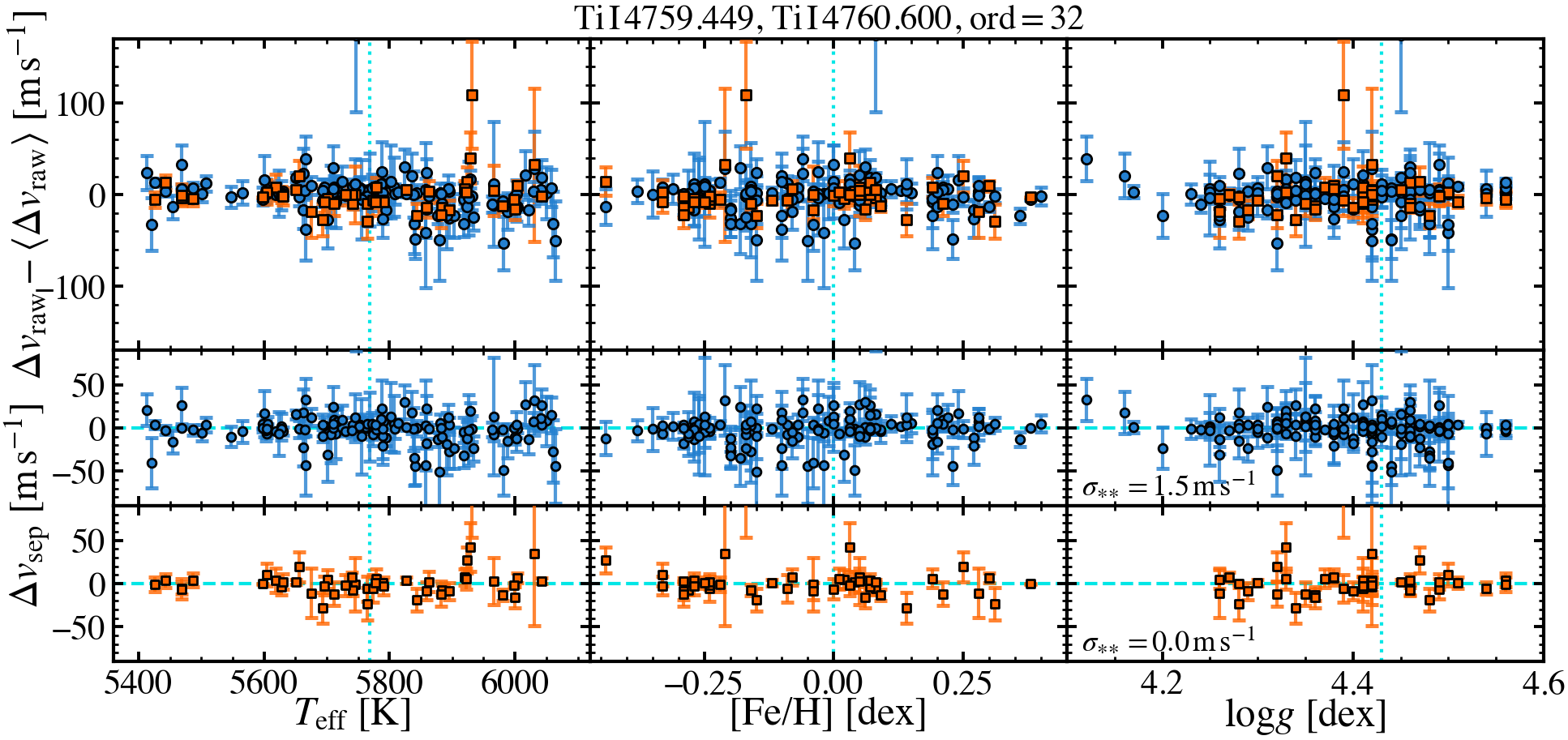
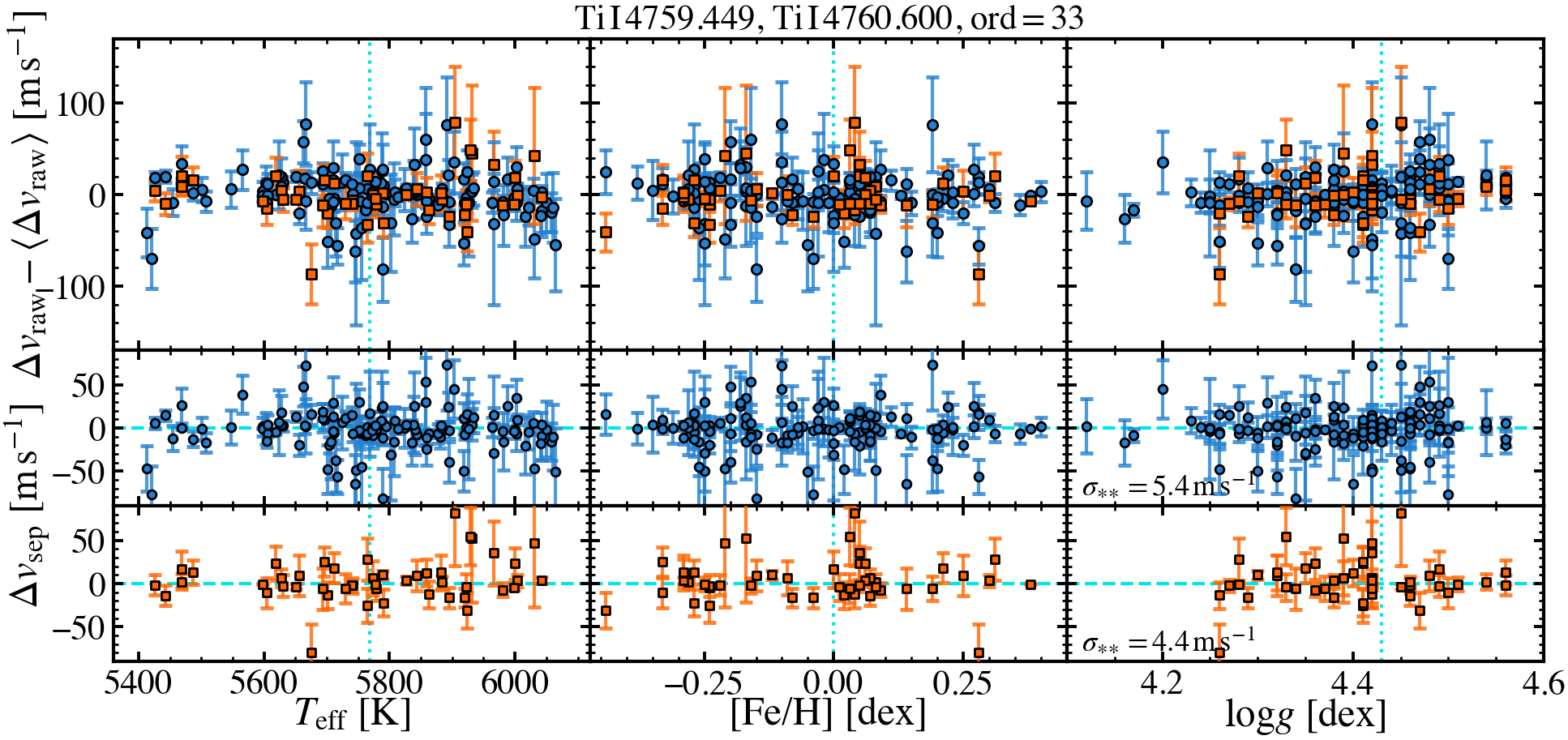
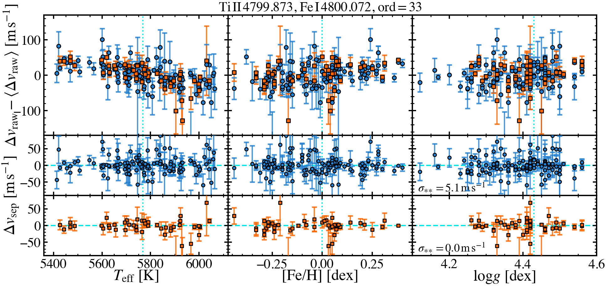
Figure S3 (continued): Variation in line pair separations.

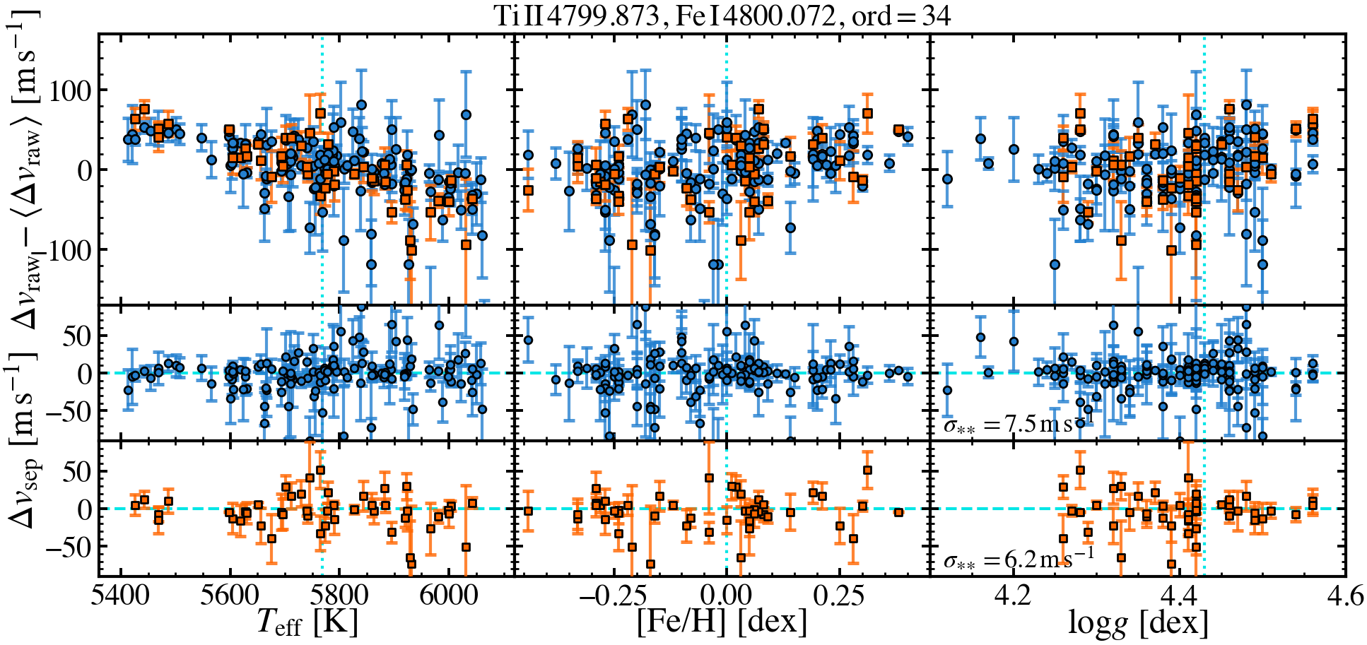
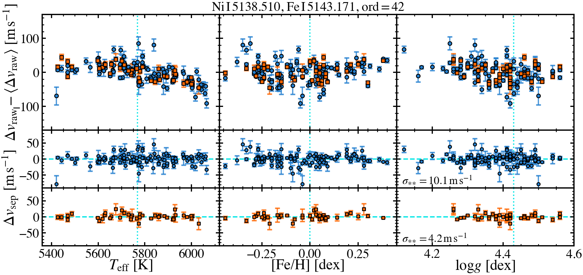
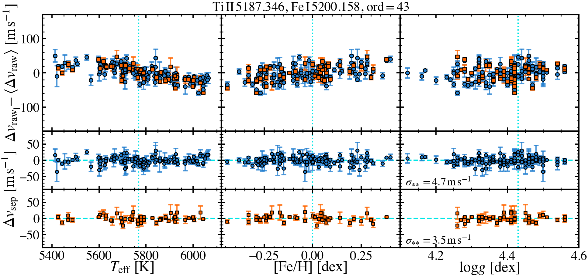
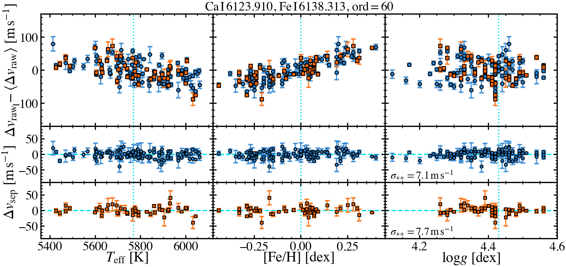
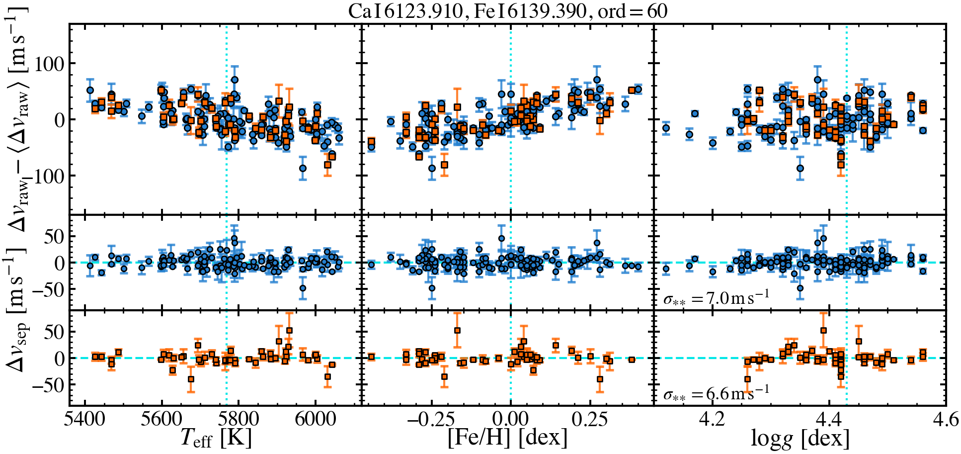
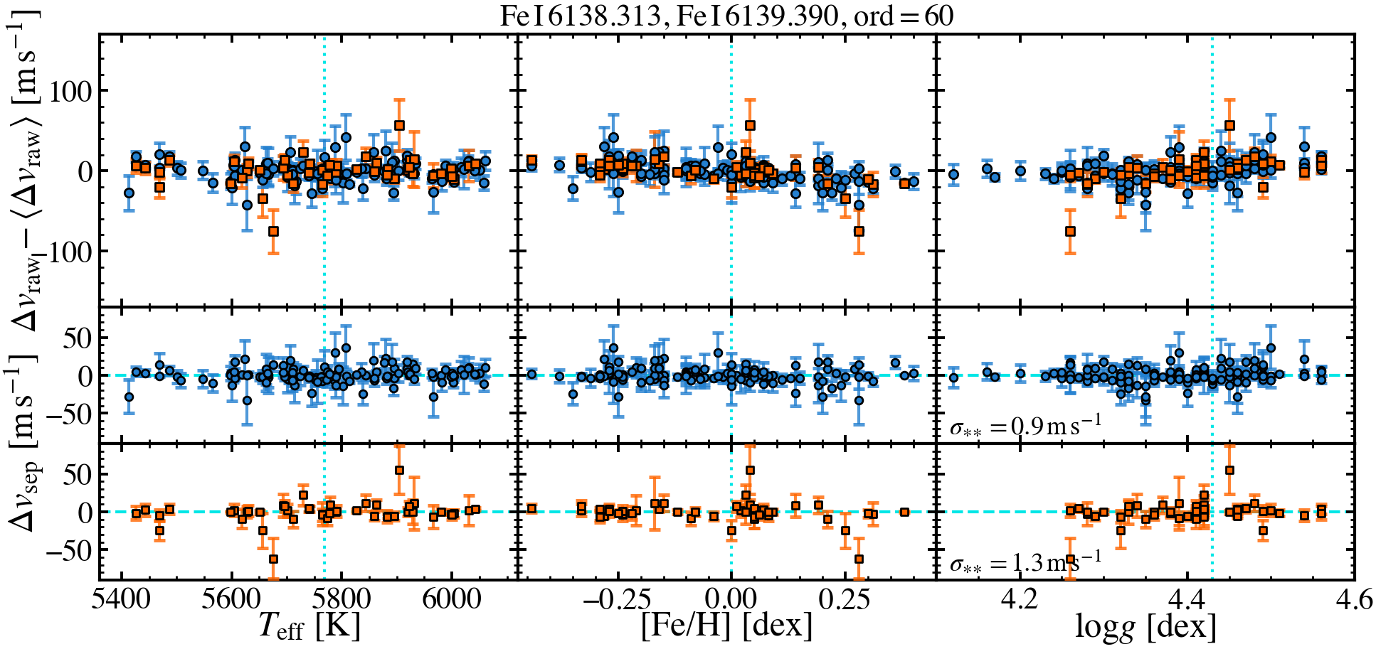
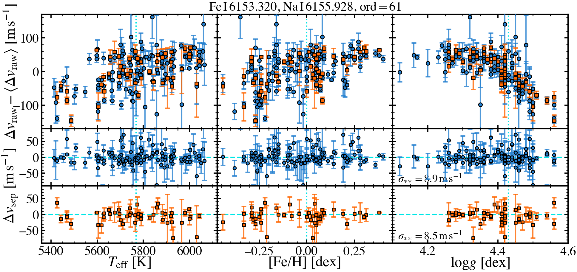
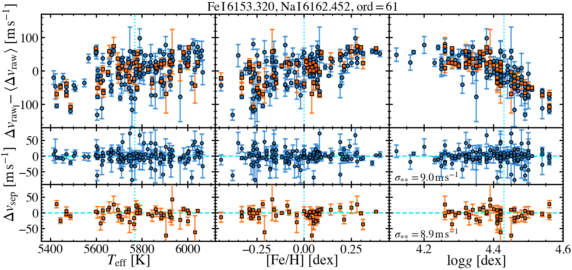
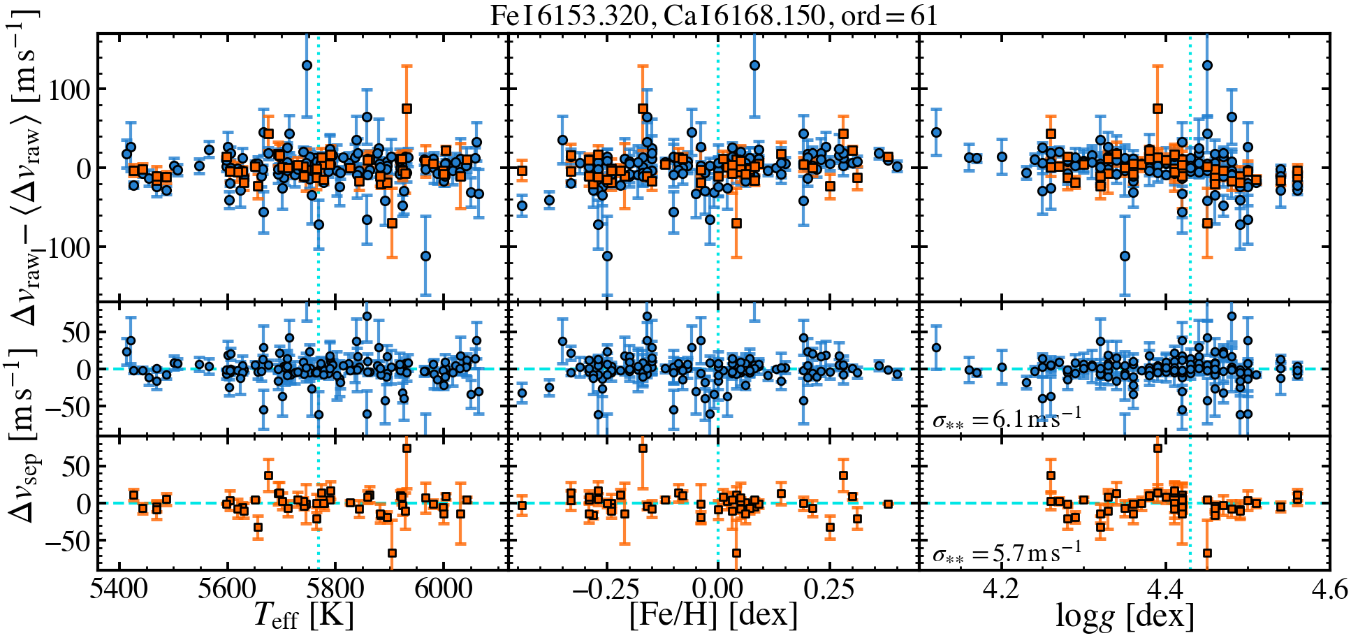
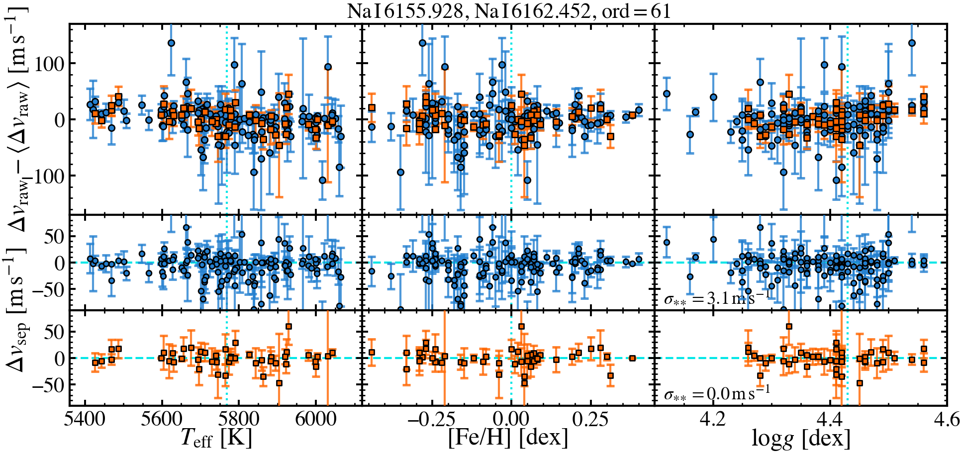
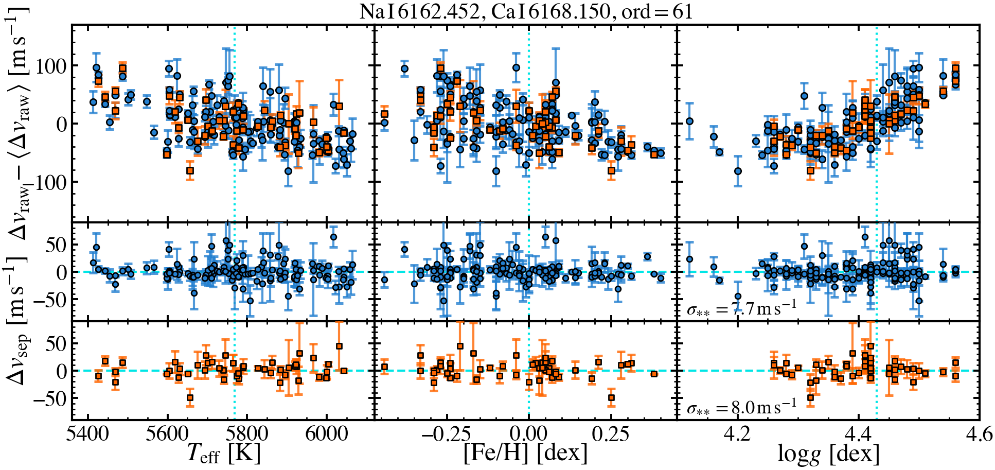
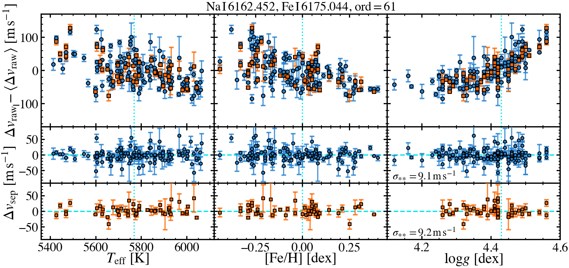
Figure S3 (continued): Variation in line pair separations.

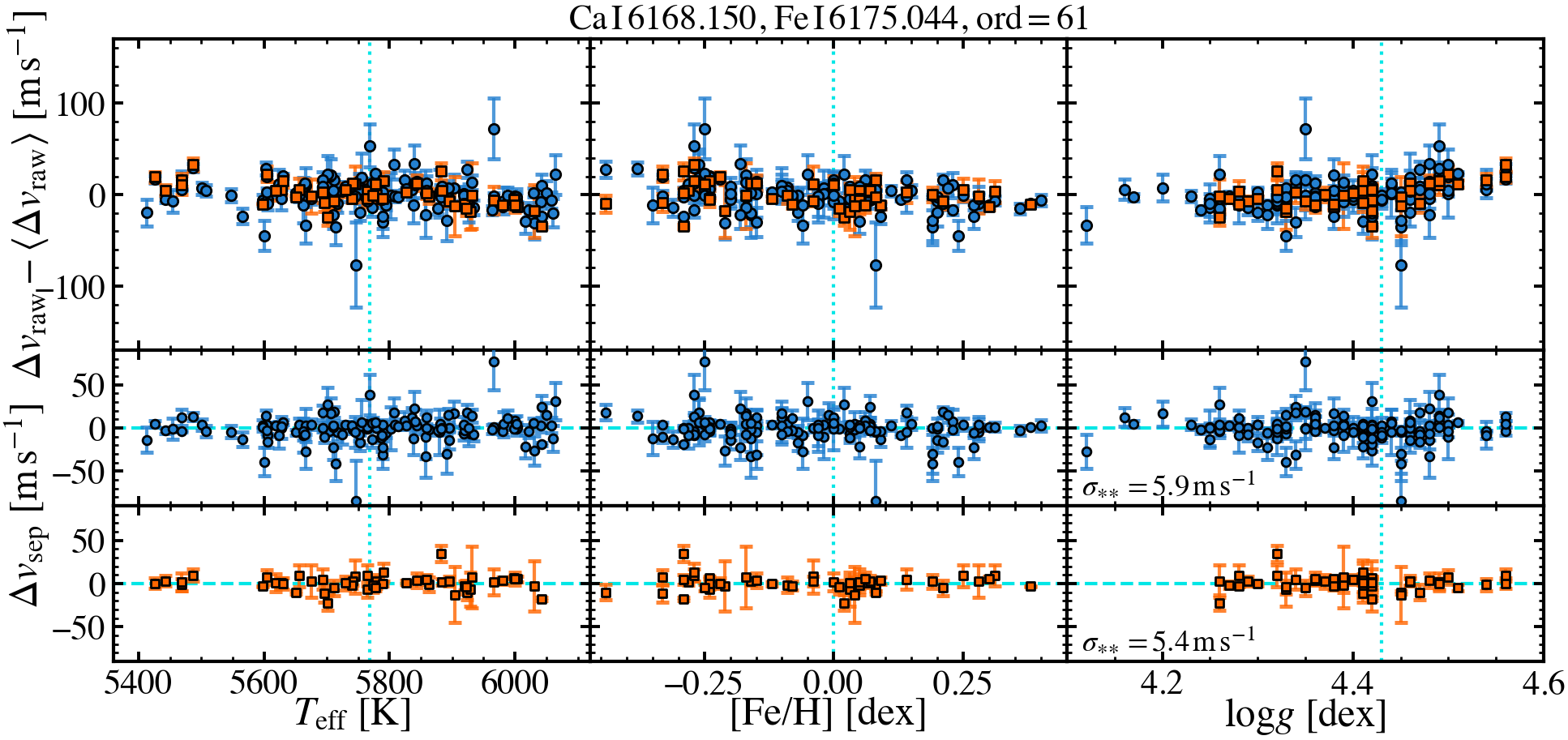
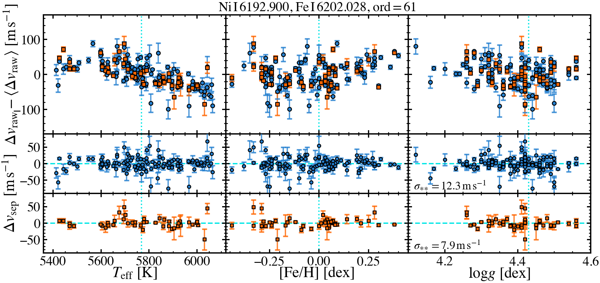
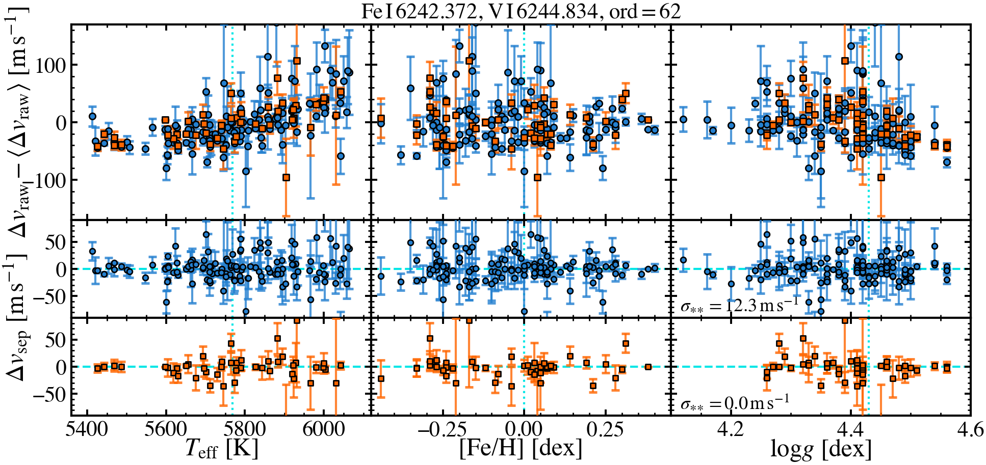
Figure S3 (continued): Variation in line pair separations.

Figure S3 (continued): Variation in line pair separations.

Figure S3 (continued): Variation in line pair separations.

Figure S3 (continued): Variation in line pair separations.

A possible alternative approach to estimating $\Delta v^{i}_{\rm model}$ would be to derive it from simulated stellar line profiles. Numerical simulations of stellar atmospheres in three dimensions  (?, ?, ?, ?) model the convective motions outlined above and allow individual spectral line profiles to be synthesised. In principal, a synthetic profile of an individual line would replace the empirical model, $\Delta v^{i}_{\rm model}$, in our approach and could be fitted to the observed line. However, such models are not accurate enough to avoid systematic effects in comparing pairs of lines in different (similar) stars at the  $<$$\sim$ 5 m s^-1 level required; the inaccuracies are up to an order of magnitude larger  (?). In addition, no synthetic profiles at suitable stellar parameters are available for the 22 lines we use. We prefer the empirical approach described above because it incorporates all contributions to variations in the pair separation, including, for example, from weak blends, and ensures we measure and account for any remaining star-to-star variance around the model (as characterised by $\sigma^{i}_{**}$).

A previous study  (?) found that $\Delta v^{i}_{\rm raw}$ did not vary across exposures of any individual star. Some of the 17 stars had $>$50 high-SNR exposures available, covering more than a decade of observations, and spanning the change in HARPS optical fibres in mid-2015. The $\Delta v^{i}_{\rm raw}$ measurements before the fibre change were self-consistent, as were those after the fibre change, but the weighted mean values from before and after the change disagreed by  $<$$\sim$ 30 m s^-1. A similar disagreement was found in the weighted mean $\Delta v^{i}_{\rm raw}$ for the two ‘instances’ of pairs that appeared in two different echelle orders of the spectrograph  (?). To account for these differences, the weighted mean $\Delta v^{i}_{\rm raw}$ was used in the modelling (averaged across exposures of the same star) where $i$ represents each instance of a pair before or after the fibre change. That is, for a single pair, up to 4 different models were used. Fig. S2 shows the result of subtracting the model from the measured $\Delta v^{i}_{\rm raw}$ values of a single line pair as a function of metallicity for all 130 stars in the larger ‘solar type’ sample  (?), with panels B and C showing the pre- and post-fibre change results separately. Fig. S3 shows the results for all 17 line pairs used here and all three stellar parameters ($T_{\rm eff}$, [Fe/H] and $\log g$).

For all but 4 of the 17 pairs used to measure $\Delta\alpha/\alpha$, the statistical uncertainties alone could not explain the scatter around the model. The additional, star-to-star scatter, $\sigma^{i}_{**}$, has been investigated elsewhere  (?) and was found to be mainly astrophysical in origin, although a small component may be due to instrumental and calibration effects. The distribution of $\sigma^{i}_{**}$ for the 17 pairs [and the larger sample of 229 pairs  (?)] peaks around $\approx$8 m s^-1, with a range of $\approx$4–15 m s^-1 for most pairs. There is no evidence for variations in $\sigma^{i}_{**}$ with $T_{\rm eff}$, [Fe/H] and $\log g$ within the ‘solar analogue’ range ($\pm$300K, $\pm$0.3 dex, $\pm$0.4 dex)  (?), so we treat $\sigma^{i}_{**}$ as constant for all solar analogue stars for a given pair $i$. We expect that the models  (?, ?) should be applicable to all solar analogue stars.

Deriving $\Delta\alpha/\alpha$ from pair velocity separations

We calculated the $\Delta\alpha/\alpha$ values from the $\Delta v^{i}_{\rm sep}$ and $\sigma^{i}_{**}$ values measured previously  (?, ?). The (up to 4) different measurements of $\Delta v^{i}_{\rm sep}$ of a single pair, in a single star, were generally consistent with each other. Therefore, these were averaged to produce a single $\Delta v^{i}_{\rm sep}$ value for each pair, $i$, per star. The weights in this average were taken as the (inverse square) statistical uncertainties, which are themselves derived from the weighted mean across all exposures of the star (see above). The $\sigma^{i}_{**}$ values were not used in this average, because they are not meaningful for a single star, and are generally very similar for the different instances of a pair, both before and after the fibre change. Including them in the weights has a negligible effect on the $\Delta\alpha/\alpha$ results. Similarly, to represent the $\sigma^{i}_{**}$ value of a pair in a single star, we used the average of the (up to 4) values for the two instances and fibre-change epochs.

For each star, the $\Delta v^{i}_{\rm sep}$ values were converted to $\Delta\alpha/\alpha$ using equation (1) applied to a line pair $i$, i.e.

$$\left(\frac{\Delta\alpha}{\alpha}\right)_{i}=-\frac{\Delta v^{i}_{\rm sep}}{c}\frac{\Delta Q}{2}\,,$$ (S1)

where $\Delta Q$ is the difference in $Q$ values of the two lines comprising the pair (with the same sign convention as the velocity difference, i.e. red minus blue). This has statistical and star-to-star uncertainties corresponding to those derived for $\Delta v^{i}_{\rm sep}$ above, plus an uncertainty in $\Delta Q$ derived from the uncertainties for individual lines  (?). Within these uncertainties, which are dominated by those in $\Delta v^{i}_{\rm sep}$, we found consistency amongst the $(\Delta\alpha/\alpha)_{i}$ values for all pairs $i$ for individual stars. We therefore averaged these together to determine the $\Delta\alpha/\alpha$ value for each star shown in Fig. 2; these are reported in Table S1. A Monte Carlo simulation was used to derive this and its statistical and systematic error components: $10^{5}$ realisations of $(\Delta\alpha/\alpha)_{i}$ were calculated, drawn from a Gaussian distribution in $\Delta v^{i}_{\rm sep}$ with width equal to the quadrature sum of its statistical and star-to-star uncertainties, $\sigma^{i}_{\rm tot}$, and with $\Delta Q$ drawn from a uniform distribution. We chose the latter because the $Q$ uncertainties are not derived in a statistical manner, instead representing the range of plausible theoretical expectations  (?). Multiple pairs can share the same lines, so uncertainties in their $Q$ values cause correlated errors in $\Delta\alpha/\alpha$. We therefore derived the $\Delta Q$ distributions from shared distributions of $Q$ for the shared lines. The $\Delta\alpha/\alpha$ value for each star was calculated as the weighted mean over the realisations, using $1/(\sigma^{i}_{\rm tot})^{2}$ as weights (including uncertainties in $\Delta Q$ had negligible effect). The statistical and systematic uncertainties shown in Fig. 2 were derived using the same process, but with the appropriate error components removed, then comparing the quadrature difference between the resulting distribution of $\Delta\alpha/\alpha$ and the original one (with all error components included).

Table S2: Stellar parameters and $\Delta\alpha/\alpha$ values. The first column provides the star names, with the (J2000) right-ascensions and declinations in the second and third columns. The stellar parameters are in the fourth, fifth and sixth columns. The values and statistical uncertainties in $\Delta\alpha/\alpha$ are provided in the seventh and eighth columns, and the final column provides the systematic error derived from the star-to-star scatter values for the 17 line pairs and the $Q$ coefficient uncertainties  (?).

Objects	RA (J2000)	Dec. (J2000)	$T_{\rm eff}$	[Fe/H]	$\log g$	$\Delta\alpha/\alpha$	$\sigma_{\rm stat}$	$\sigma_{\rm sys}$
	(hh:mm:ss)	(dd:mm:ss)	(K)	(dex)	(dex)	(ppb)	(ppb)	(ppb)
Sun	—	—	5772	$0.00$	4.44	$-15.4$	26.6	36.6
HD 19467	03:07:18.58	$-$13:45:42.4	5753	$-0.07$	4.30	$70.1$	42.5	36.9
HD 20782	03:20:03.58	$-$28:51:14.7	5773	$-0.09$	4.39	$-40.5$	30.3	33.0
HD 30495	04:47:36.29	$-$16:56:04.0	5857	$-0.02$	4.50	$-67.2$	209.2	99.8
HD 45184	06:24:43.88	$-$28:46:48.4	5863	$0.04$	4.42	$25.6$	9.6	34.1
HD 45289	06:24:24.35	$-$42:50:51.1	5710	$0.03$	4.25	$30.8$	25.2	36.0
HD 76151	08:54:17.95	$-$05:26:04.0	5787	$0.03$	4.43	$-138.3$	45.6	51.1
HD 78429	09:06:38.83	$-$43:29:31.1	5740	$0.05$	4.27	$10.8$	15.2	31.3
HD 78660	09:09:53.86	$+$14:27:24.3	5788	$-0.03$	4.39	$-224.4$	104.9	45.4
HD 138573	15:32:43.65	$+$10:58:05.9	5745	$-0.04$	4.41	$158.2$	191.7	52.6
HD 140538	15:44:01.82	$+$02:30:54.6	5693	$0.05$	4.46	$-9.4$	26.8	36.9
HD 146233	16:15:37.27	$-$08:22:10.0	5826	$0.06$	4.42	$35.1$	7.6	30.0
HD 157347	17:22:51.29	$-$02:23:17.4	5730	$0.03$	4.42	$10.8$	21.2	33.1
HD 171665	18:37:12.84	$-$25:40:16.6	5725	$-0.10$	4.46	$-109.2$	56.6	40.0
HD 183658	19:30:52.72	$-$06:30:51.9	5824	$0.06$	4.46	$90.3$	80.3	69.9
HD 220507	23:24:42.12	$-$52:42:06.8	5701	$0.02$	4.26	$61.9$	37.1	36.3
HD 222582	23:41:51.53	$-$05:59:08.7	5802	$0.00$	4.35	$84.8$	134.3	42.1

The ensemble weighted mean $\Delta\alpha/\alpha$ in equation (3), averaged over all stars, was calculated with a similar Monte Carlo approach as above. This is because, in addition to lines (and therefore $Q$s) being shared between pairs, the star-to-star scatter terms, $\sigma^{i}_{**}$, are shared between both pairs and stars. If these factors are ignored, the weighted mean value of $\Delta\alpha/\alpha$ in equation (3) is only negligibly affected, but the systematic error term is underestimated by $\sim$15%.

Recovery of a large artificial $\Delta\alpha/\alpha$ signal

The analysis procedure is completely automated, but the values of some parameters in the algorithms must be chosen to balance its sensitivity to $\Delta\alpha/\alpha$ with its ability to reject outliers. An individual line measurement is rejected if it deviates by more than 3 times its statistical uncertainty from the expected (i.e. model) offset from the laboratory wavelength (see above). If $\Delta\alpha/\alpha$ is much larger than the uncertainties in one star, a line in its spectrum with a large $\left|Q\right|$ may be rejected. For example, the Ni i 6192.900 line has $Q=0.18$  (?) so a ‘large’ $\Delta\alpha/\alpha$ of $+500$ ppb would shift it bluewards by $\approx$100 m s^-1, which is $\sim$4 times larger than the typical measurement uncertainty from a single HARPS exposure, i.e. $\sim$25 m s^-1. Therefore, measurements of the line would be rejected in most exposures by our analysis procedure. However, lines with smaller $\left|Q\right|$ would be less likely to be rejected. That is, we expect our analysis procedure to have reduced sensitivity to large differences in $\alpha$ between stars, on average.

To test the response of our analysis procedure to such large $\Delta\alpha/\alpha$ signals, we shifted the measured wavelengths of the 22 lines for 8 of the 17 stars by amounts corresponding to $\Delta\alpha/\alpha=+100$ ppb (equation 1). We applied the analysis procedure again, but removed the 8 shifted stars from the determination of $\Delta v^{i}_{\rm model}$; this prevents the artificial shifts from affecting the models and $\sigma^{i}_{**}$ calculations. Fig. S4 shows the change in $\Delta\alpha/\alpha$ for each star from the original values in Fig. 2; Table S3 provides the numerical values. The weighted mean $\Delta\alpha/\alpha$ for the shifted stars changed by $+86$ ppb from the original value, with a new total uncertainty of 19 ppb (cf. original value of 18 ppb; combining statistical and systematic uncertainties in quadrature). That is, we find that $86\pm 19$% of the $+100$ ppb input signal was recovered. Nevertheless, Fig. S4 also shows that the change in $\Delta\alpha/\alpha$ for HD 171665 and HD 220507 was $>+$140 ppb, while for HD 138573 it was $-175$ ppb. These deviations from the expected average response are due to lines and pairs being rejected in the analysis procedure because of the large $\Delta\alpha/\alpha$ signal. The effect for HD 138573 is particularly large because only one exposure was available. The unshifted stars show very little change in $\Delta\alpha/\alpha$; these are due to small changes in $\Delta v^{i}_{\rm model}$ because the 8 shifted stars were removed (out of 130 stars in total) from its determination.

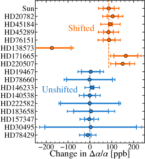
Figure S4: Change in $\Delta\alpha/\alpha$ in response to an artificial signal. The measured line wavelengths for the 8 shifted stars (orange points) were altered by amounts corresponding to $\Delta\alpha/\alpha=+100$ ppb, while those for the unshifted stars (blue points) were not altered. The inner (large) and outer (small) error bars have the same meaning as in Fig. 2 (i.e. statistical and total uncertainties, respectively) but for the new value of $\Delta\alpha/\alpha$ for each star. The dashed vertical lines indicate the change in the weighted means for the shifted (orange) and unshifted (blue) samples.

Table S3: Change in $\Delta\alpha/\alpha$ in response to an artificial signal. The first column provides the star names and the second column states whether the measured line wavelengths for each star were altered using the artificial signal of $\Delta\alpha/\alpha=+100$ ppb. The change in $\Delta\alpha/\alpha$ from the original results in Fig. 2 and Table S2 is shown in the third column. The final two columns show the new $1\sigma$ statistical and systematic uncertainties.

Objects	Shifted?	Change in $\Delta\alpha/\alpha$	$\sigma_{\rm stat}$	$\sigma_{\rm sys}$
		(ppb)	(ppb)	(ppb)
Sun	Yes	$85.9$	25.2	39.5
HD 19467	No	$3.2$	42.5	40.3
HD 20782	Yes	$103.8$	25.6	38.3
HD 30495	No	$4.3$	209.5	103.1
HD 45184	Yes	$93.1$	8.8	43.7
HD 45289	Yes	$84.5$	22.4	40.2
HD 76151	Yes	$87.8$	27.1	43.1
HD 78429	No	$-10.0$	15.2	34.7
HD 78660	No	$-1.8$	105.0	49.8
HD 138573	Yes	$-175.1$	87.7	41.1
HD 140538	No	$-0.9$	26.8	39.8
HD 146233	No	$10.0$	7.6	32.7
HD 157347	No	$-3.6$	21.1	36.9
HD 171665	Yes	$163.1$	54.5	44.2
HD 183658	No	$4.9$	79.8	73.6
HD 220507	Yes	$149.4$	32.0	44.6
HD 222582	No	$-1.8$	133.7	45.1

References

- 1. R. Lange, et al., Phys. Rev. Lett. 126, 011102 (2021).
- 2. S. M. Kotuš, M. T. Murphy, R. F. Carswell, Mon. Not. Roy. Astron. Soc. 464, 3679 (2017).
- 3. M. T. Murphy, K. L. Cooksey, Mon. Not. Roy. Astron. Soc. 471, 4930 (2017).
- 4. M. T. Murphy, et al., Astron. Astrophys. 658, A123 (2022).
- 5. A. Hees, et al., Phys. Rev. Lett. 124, 081101 (2020).
- 6. J. Hu, et al., Mon. Not. Roy. Astron. Soc. 500, 1466 (2021).
- 7. V. A. Dzuba, V. V. Flambaum, J. K. Webb, Phys. Rev. Lett. 82, 888 (1999).
- 8. D. Dravins, Ann. Rev. Astron. Astrophys. 20, 61 (1982).
- 9. J. I. González Hernández, et al., Astron. Astrophys. 643, A146 (2020).
- 10. V. A. Dzuba, V. V. Flambaum, M. T. Murphy, D. A. Berke, Phys. Rev. A 105, 062809 (2022).
- 11. D. A. Berke, M. T. Murphy, C. Flynn, F. Liu, Mon. Not. Roy. Astron. Soc., accepted, doi:10.1093/mnras/stac2458, arXiv:2210.08275 (2022).
- 12. D. A. Berke, M. T. Murphy, C. Flynn, F. Liu, Mon. Not. Roy. Astron. Soc., accepted, doi:10.1093/mnras/stac2037, arXiv:2210.08276 (2022).
- 13. Materials and methods are available as supplementary materials.
- 14. M. Mayor, et al., The Messenger 114, 20 (2003).
- 15. T. Wilken, et al., Mon. Not. Roy. Astron. Soc. 405, L16 (2010).
- 16. D. Milaković, L. Pasquini, J. K. Webb, G. Lo Curto, Mon. Not. Roy. Astron. Soc. 493, 3997 (2020).
- 17. A. Coffinet, C. Lovis, X. Dumusque, F. Pepe, Astron. Astrophys. 629, A27 (2019).
- 18. J. W. Brault, Mikrochimica Acta 1, 215 (1987).
- 19. M. Laverick, et al., Astron. Astrophys. 612, A60 (2018).
- 20. D. A. Berke, Zenodo (2022); doi: 10.5281/zenodo.7196771, http://doi.org/10.5281/zenodo.7196771
- 21. D. A. Berke, M. T. Murphy, C. Flynn, F. Liu, Zenodo (2022); doi: 10.5281/zenodo.7196796, http://doi.org/10.5281/zenodo.7196796
- 22. M. T. Murphy, et al., Zenodo (2022); doi: 10.5281/zenodo.7196515, http://doi.org/10.5281/zenodo.7196515
- 23. R. D. Haywood, et al., Mon. Not. Roy. Astron. Soc. 457, 3637 (2016).
- 24. L. Casagrande, et al., Astron. Astrophys. 530, A138 (2011).
- 25. B. Nordström, et al., Astron. Astrophys. 418, 989 (2004).
- 26. ESO Science Archive Facility, http://archive.eso.org/eso/eso_archive_main.html.
- 27. A. Prša, et al., Astron. J. 152, 41 (2016).
- 28. G. Rupprecht, et al., The exoplanet hunter HARPS: performance and first results (2004), vol. 5492 of Society of Photo-Optical Instrumentation Engineers (SPIE) Conference Series, pp. 148–159.
- 29. X. Dumusque, Astron. Astrophys. 620, A47 (2018).
- 30. D. Dravins, Astron. Astrophys. 492, 199 (2008).
- 31. A. Nordlund, D. Dravins, Astron. Astrophys. 228, 155 (1990).
- 32. M. Asplund, Å. Nordlund, R. Trampedach, C. Allende Prieto, R. F. Stein, Astron. Astrophys. 359, 729 (2000).
- 33. M. Asplund, N. Grevesse, A. J. Sauval, P. Scott, Ann. Rev. Astron. Astrophys. 47, 481 (2009).
- 34. Z. Magic, et al., Astron. Astrophys. 557, A26 (2013).
Acknowledgments
We thank Dainis Dravins for discussions about potential astrophysical systematic errors.
Funding: M.T.M., F.L. and C.L. acknowledge the support of the Australian Research Council through Future Fellowship grant FT180100194. V.A.D. and V.V.F. acknowledge the Australian Research Council for support through grants DP190100974 and DP200100150. OzGrav is funded by the Australian Government through the Australian Research Council Centres of Excellence funding scheme.
Author contributions: M.T.M. conceived the stellar twins technique, acquired funding, supervised the project, calculated the values and wrote the draft manuscript. D.A.B. wrote the software, performed the velocity shift measurements and analysis, and curated all data. F.L., C.F. and C.L. assisted with the methodology, analysis and validation of results. V.A.D. and V.V.F. calculated the sensitivity coefficients (). All authors reviewed and revised the manuscript.
Competing interests: The authors declare no competing interests.
Data and materials availability: This work is based on observations obtained from the ESO Science Archive Facility and collected at the European Southern Observatory under ESO programme(s) listed in Table S1. The observations are available from the ESO Science Archive facility: http://archive.eso.org/eso/eso_archive_main.html. Our software for measuring the line wavelengths, and computing the line pair separations and models is available on Zenodo (?). Tables of the lines used in this study, their laboratory wavelengths, our measured and model offsets from those values, and our measured line pair separations, models and values are available on Zenodo (?). Our software for computing in this work is available on Zenodo (?). The stellar parameters and our measured values and uncertainties are listed in Table S2.