Breaking the quantum Cramér-Rao bound with non-Markovian memory effects

Abstract

Linear optics provides versatile means to simulate and control the dynamics of open quantum systems. Here, the polarization and frequency of photons often represent the system and its environment, respectively. Recently, the photon’s path degree of freedom and the effects of interference have been considered as well, giving rise to the concept of “open system interference”. Such models have been shown to beat traditional parameter estimation schemes in certain scenarios. In this work, we study the sensitivity of non-Markovian memory effects arising from an open system Mach-Zehnder interferometer. Our protocol provides an alternative way to get around the quantum Cramér-Rao theorem, proving itself a noteworthy option for more conventional parameter estimation protocols.

I Introduction

Open quantum systems are characterized by their interaction with the environment petru . Due to these system-environment interactions, open systems typically become classical, which is harmful for quantum technologies using realistic quantum systems as their building blocks. However, the quantum-to-classical transition does not always occur monotonically, as open systems may sometimes regain information previously lost in the environment. Such dynamics is often dubbed non-Markovian nm_1 ; nm_2 ; nm_3 ; nm_4 ; nm_5 ; nm_6 . Great efforts have been made to understand quantum non-Markovianity and harness non-Markovian memory effects in noisy quantum applications. For example, non-Markovianity has been shown to enhance the performance of Deutsch-Josza algorithm dj , quantum teleportation tele_1 ; tele_2 , and quantum key distribution qkd .

Linear optics provides a proof-of-concept testbed in which to study open-system dynamics lin_opt_1 ; lin_opt_2 ; lin_opt_3 ; lin_opt_4 ; lin_opt_5 ; lin_opt_6 ; lin_opt_7 ; lin_opt_8 . Here, the polarization degree of freedom of photons is often interpreted as the open quantum system, their own frequency plays the role of an environment, and the system-environment interaction is implemented in a birefringent medium. Although the total polarization-frequency system is closed and undergoes unitary dynamics, one obtains nonunitary polarization dephasing when averaging over the frequency. Most notably, this model corresponds directly to a qubit coupled to bosonic bath petru ; lin_opt_8 ; suominen .

Recent works related to linear optical open-system simulators have also considered the path degree of freedom and the interactions induced by beam splitters mznm ; hom . “Open system interferometer” (coined in mznm ) refers to interferometers where the polarization dynamics affects interference and/or vice versa. In Ref. mznm , the Authors were interested in the open-system (polarization) dynamics caused by coherent mixing of different dephasing channels, how it affects the interference within a Mach-Zehnder interferometer, and how the interference, in turn, affects the following dynamics. It was found that, in this context too, superposing different evolution paths can induce memory effects (cf. int_eng ). Perhaps more interestingly, it was also shown that monitoring such dynamics can be used in parameter estimation outside of the interferometer’s more common working region, i.e., when the path probabilities no longer carry information about the parameter of interest.

In this paper, we study non-Markovian memory effects arising from interacting subenvironments (frequency and path) within an open system interferometer. Prior works have studied similar effects of inter-environmental correlations (see, e.g., Refs. ent_env_1 ; ent_env_2 ), but our motivation is different. Here, we are interested if the open system interferometer can beat its traditional counterpart also in the interferometric region by harnessing memory effects. We numerically analyze the memory effects’ sensitivity with respect to the memory-inducing parameter, i.e., the path difference of an unbalanced Mach-Zehnder interferometer, and make an exciting discovery. Concentrating on the global features of a quantum dynamical map allows us to break the quantum Cramér-Rao bound (QCRB) qcrb which, until quite recently beyond_1 ; beyond_2 ; beyond_3 ; beyond_4 ; beyond_5 , was believed to give the ultimate measurement precision. Our results therefore have twofold significance: They help to better understand non-Markovian dynamics of open quantum systems while simultaneously providing a powerful tool for quantum sensing and quantum metrology.

This paper is organized as follows. In Section II, we go through the necessary background of open quantum systems, non-Markovianity, and parameter estimation. In Section III, we introduce our protocol. The main results of this paper are presented in Section IV with fixed example parameters. Section V concludes the paper.

II Open quantum systems, non-Markovianity, and parameter estimation

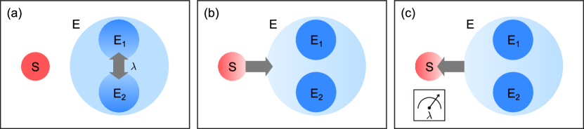
Figure 1: Schematic picture of parameter estimation with memory effects. (a) Information about $\lambda$ (path difference in the photonic realization) is imprinted on the environment $E$ with the subenvironments $E_{1}$ and $E_{2}$ (frequency and path) interacting. (b) The open system $S$ (polarization) starts interacting with $E$. (c) If memory effects are detected, we can estimate $\lambda$.

A quantum system $S$ is said to be open if it interacts with some other system, dubbed its environment $E$ petru . As a consequence, information carried by $S$ typically transforms into correlations between $S$ and $E$. Trace distance $D_{tr}(\rho_{1},\rho_{2})=\frac{1}{2}\text{tr}|\rho_{1}-\rho_{2}|$ provides an intuitive way to characterize this information flow, as it is directly proportional to the distinguishability of two (open-system) states $\rho_{1}$ and $\rho_{2}$ chuang ; $S$ carries less information if $\rho_{1}$ and $\rho_{2}$ become less distinguishable under some environment-induced mapping $\rho\mapsto\Phi(\rho)$.

The dynamics of open quantum systems is often described by completely positive and trace-preserving (CPTP) maps, or channels $\Phi$, under which the trace distance can never increase, i.e., $D_{tr}\big{(}\Phi(\rho_{1}),\Phi(\rho_{2})\big{)}\leq D_{tr}(\rho_{1},\rho_{2})$ chuang . However, because the total system $SE$ is closed, the open system $S$ may sometimes regain some of the previously lost information. In such situations the trace distance can temporally increase, though never exceeding its initial value. According to the Breuer, Laine, and Piilo (BLP) definition, such nonmonotonic behavior of trace distance indicates non-Markovian dynamics and the presence of memory effects blp .

We note that there is no sole, universally agreed definition of quantum (non-)Markovianity nm_1 ; nm_2 ; nm_3 ; nm_4 ; nm_5 ; nm_6 ; blp ; teittinen ; modi ; budini . Still, the revivals of trace distance coincide with many other indicators of non-Markovianity teittinen . Most notably—and in the case of single-qubit dephasing, which we will be dealing with—the increase of trace distance coincides with the violation of completely positive (CP) divisibility nm_1 .

The BLP-measure of quantum non-Markovianity is more formally defined as

$$\mathcal{N}(\Phi)=\max_{\rho_{1,2}(0)}\int_{\sigma>0}dt\sigma\big{(}t,\rho_{1,2}(0)\big{)},$$ (1)

where $\sigma(t,\rho_{1,2}(0)\big{)}=\frac{d}{dt}D_{tr}\big{(}\rho_{1}(t),\rho_{2}(t)\big{)}$. Hence, the BLP-measure simply gives the total increase of trace distance upon the whole time evolution induced by the channel $\Phi$, maximized with respect to the initial state pair $\rho_{1,2}(0)$. In this work, we simulate these memory effects in a quantum optical setting and analyze their sensitivity in parameter estimation.

In sensitivity analysis, one is often interested in how some $\lambda$-dependent observable $O(\lambda)$ changes with small changes of $\lambda$. Here, $\lambda$ is the parameter being estimated. For small enough changes $|\delta\lambda|<<1$, we can write

$$\langle O(\lambda+\delta\lambda)\rangle\approx\langle O(\lambda)\rangle+\frac{\partial\langle O(\lambda)\rangle}{\partial\lambda}\delta\lambda,$$ (2)

where $\langle O\rangle$ denotes the observable’s expectation value. The difference $|\langle O(\lambda+\delta\lambda)\rangle-\langle O(\lambda)\rangle|$ can be experimentally detected if it is greater than the standard deviation $\Delta O:=\sqrt{\langle O^{2}\rangle-\langle O\rangle^{2}}$; Smaller difference could be interpreted as a result of the observable’s intrinsic spread.

Thus, $\delta\lambda$ needs to satisfy

$$|\delta\lambda|\geq\frac{\Delta O}{|\frac{\partial\langle O(\lambda)\rangle}{\partial\lambda}|}$$ (3)

to be experimentally detectable sensitivity . The value $\delta\lambda^{\prime}$ that saturates the inequality is called the observable’s sensitivity. Assuming parameter-independent measurements beyond_1 , the sensitivity is bounded from below by the QCRB paris ,

$$|\delta\lambda^{\prime}|\geq\frac{1}{\sqrt{MH(\lambda)}}.$$ (4)

Here, $M$ is the number of measurements and $H(\lambda)$ is the quantum Fisher information which, for pure states $|\psi\rangle$, can be written as paris

$$H(\lambda)=4(\langle\partial_{\lambda}\psi|\partial_{\lambda}\psi\rangle-|\langle\partial_{\lambda}\psi|\psi\rangle|^{2}),$$ (5)

where $|\partial_{\lambda}\psi\rangle=\partial|\psi(\lambda)\rangle/\partial\lambda$.

III Protocol

Our parameter estimation protocol goes as follows. First, we encode the parameter $\lambda$ into the environment with inter-environmental interactions. We then let the open system interact with the environment and monitor its dynamics. If we detect memory effects, we are able to estimate $\lambda$. In this paper, we are especially interested in how small changes $\delta\lambda$ affect the memory effects. The protocol is illustrated in Fig. 1.

The protocol can be realized in linear optical framework. Here, the polarization degree of freedom of a single photon is interpreted as the open system, and its path and frequency act as the environment. The parameter we are interested in is the path difference of an unbalanced Mach-Zehnder interferometer.

The polarization starts in the pure state $|\psi(0)\rangle=C_{H}|H\rangle+C_{V}|V\rangle$ with $C_{H}$ ($C_{V}$) denoting the photon’s probability amplitude to be in the horizontal (vertical) state. The total initial state of the photon, containing also its frequency and path, is then

$$|\Psi_{in}\rangle=|\psi(0)\rangle\otimes\int dfg(f)|f\rangle\otimes|0\rangle,$$ (6)

where $g(f)$ is the photon’s probability amplitude to be in the frequency state $|f\rangle$.

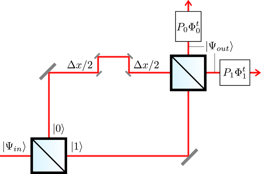
Figure 2: The setup. The two subenvironments (frequency and path) are entangled through $\Delta x$. The channels $\Phi_{0}^{t}$ and $\Phi_{1}^{t}$ with the respective weights $P_{0}$ and $P_{1}$ are then realized with birefringent crystals, e.g., quartz.

The photon is guided into a Mach-Zehnder interferometer with the arm lengths of $x_{0}$ and $x_{1}$ (see Fig. 2). Assuming 50:50 beam splitters and describing them with Hadamard operators, we obtain the output state

$$\begin{split}|\Psi_{out}\rangle=&\frac{1}{2}|\psi(0)\rangle\otimes\\ &\Bigg{[}\int dfg(f)\Big{(}e^{i2\pi fx_{0}/c}+e^{i2\pi fx_{1}/c}\Big{)}|f\rangle\otimes|0\rangle\\ &+\int dfg(f)\Big{(}e^{i2\pi fx_{0}/c}-e^{i2\pi fx_{1}/c}\Big{)}|f\rangle\otimes|1\rangle\Bigg{]},\end{split}$$ (7)

where $c$ is the speed of light. At this stage, the subenvironments represented by the path and frequency degrees of freedom have become entangled if $\Delta x:=x_{0}-x_{1}\neq 0$, while the open system (polarization) and environment are still uncorrelated.

The photon is then guided into a combination of birefringent crystals, where the polarization and frequency interact according to the unitary transformation $U(t)|\lambda\rangle\otimes|f\rangle=e^{i2\pi fn_{\lambda}t}|\lambda\rangle\otimes|f\rangle$. Here, $n_{\lambda}$ is the crystals’ refractive index corresponding to the polarization component $\lambda=H,V$. In the following, we shall write $\Delta n=n_{H}-n_{V}$.

Taking partial trace over frequency and path, we obtain the polarization state

$$\rho(t)=\begin{pmatrix}|C_{H}|^{2}&C_{H}C_{V}^{*}\kappa(t)\\ C_{H}^{*}C_{V}\kappa^{*}(t)&|C_{V}|^{2}\end{pmatrix},$$ (8)

where the decoherence function $\kappa(t)$ is the Fourier transform of the frequency distribution $|g(f)|^{2}$ lin_opt_4 . Using the Gaussian spectrum $|g(f)|^{2}=\exp\Big{[}-\frac{1}{2}\Big{(}\frac{f-\mu}{\sigma}\Big{)}^{2}\Big{]}/\sqrt{2\pi\sigma^{2}}$, we get

$$\kappa(t)=e^{i2\pi\mu\Delta nt-\frac{1}{2}(2\pi\sigma\Delta nt)^{2}}.$$ (9)

We notice that the state $\rho(t)$ does not depend on $\Delta x$. However, if we only monitor one of the exit paths $j=0,1$, we obtain the (normalized) state

$$\rho_{j}(t)=\begin{pmatrix}|C_{H}|^{2}&C_{H}C_{V}^{*}\kappa_{j}(t)\\ C_{H}^{*}C_{V}\kappa_{j}^{*}(t)&|C_{V}|^{2}\end{pmatrix},$$ (10)

where

$$\begin{split}\kappa_{j}(t)=\frac{1}{4P_{j}}\Big{[}2\kappa(t)+&(-1)^{j}\kappa\big{(}t+\Delta x/(c\Delta n)\big{)}\\ +&(-1)^{j}\kappa\big{(}t-\Delta x/(c\Delta n)\big{)}\Big{]}.\end{split}$$ (11)

$P_{j}=\frac{1}{2}\Big{\{}1+(-1)^{j}\exp\Big{[}-\frac{1}{2}(2\pi\sigma\Delta x/c)^{2}\Big{]}\cos(2\pi\mu\Delta x/c)\Big{\}}$ is the probability to detect the photon on exit path $j$.

The path-wise decoherence function $\kappa_{j}(t)$ describes how all the polarization components combine in the second beam splitter and interfere afterwards in the birefringent crystals. That is, $2\kappa(t)$ describes how the parallel components $H+H$ and $V+V$ behave, whereas $\kappa\big{(}t\pm\Delta x/(c\Delta n)\big{)}$ describes the dynamics of $H+V$ and $V+H$, each pair originating from the two paths inside the interferometer.

Associating the decoherence functions $\kappa(t)$ and $\kappa_{j}(t)$ with the channels $\Phi^{t}$ and $\Phi_{j}^{t}$, respectively, we can write the lossless polarization dynamics following the second beam splitter as

$$\rho(t) =\Phi^{t}\big{(}\rho(0)\big{)}$$ (12)

$$=P_{0}\Phi_{0}^{t}\big{(}\rho(0)\big{)}+P_{1}\Phi_{1}^{t}\big{(}\rho(0)\big{)}.$$ (13)

Our task is now to estimate $\Delta x$ by using the BLP-non-Markovianity of $\Phi_{j}^{t}$. Note that here we are guaranteed to always have valid CPTP maps. If we had dephasing of polarization also inside the interferometer, we would need to describe the final open-system dynamics with completely positive and trace-nonincreasing (CPTNI) quantum operations, as in mznm .

IV Sensitivity of memory effects

With dephasing channels, the initial state pair $|\pm\rangle=\frac{1}{\sqrt{2}}(|H\rangle\pm|V\rangle)$ generally maximizes the revivals of trace distance lin_opt_6 . With this choice, the trace distance equals the absolute value of the decoherence function. For example, $|\kappa(t)|=\text{exp}[-(2\pi\sigma\Delta nt)^{2}/2]$ decreases monotonically, making the total channel $\Phi^{t}$ in Eq. (12) Markovian. However, the channels $\Phi_{0}^{t}$ and $\Phi_{1}^{t}$ can both be Markovian (M+M), non-Markovian (nM+nM), or one Markovian, the other non-Markovian (M+nM or nM+M), as we will soon see. Here, the path difference $\Delta x$—and so, the concurrence of the environment state—acts as the source of non-Markovianity (see the Appendix for details).

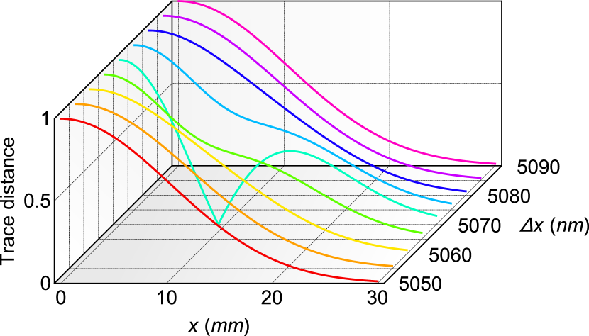
Figure 3: Trace distance dynamics of the initial state pair $|\pm\rangle$ as functions of the thickness of quartz and with different values of $\Delta x$. $\mu=c/(780\text{ nm})$, $\sigma=5.68\times 10^{11}\text{ Hz}$, and $\Delta n=0.009$.

From here on, let us focus on the channel $\Phi_{0}^{t}$. The channel $\Phi_{1}^{t}$ is handled in a similar fashion. To visualize the memory effects and their dependency on $\Delta x$, we have plotted the trace distance dynamics of the state pair $\Phi_{0}^{t}(|\pm\rangle\langle\pm|)$ in Fig. 3 with different values of $\Delta x$. With the example parameters, we see a sudden emergence of non-Markovian memory effects around $\Delta x=5070\text{ nm}$. However, in Fig. 3 we also have $P_{0}<0.01$, which means that the memory effects are extremely hard to measure.

Fig. 4—with Fig. 4(e) corresponding to Fig. 3—better illustrates the interplay of $P_{0}$ and $\mathcal{N}(\Phi_{0}^{t})$. The path probability $P_{0}$ oscillates with a frequency determined by $\mu$ and approaches 1/2 with a damping rate determined by $\sigma$. Interestingly, the BLP-non-Markovianity $\mathcal{N}(\Phi_{0}^{t})$—which is evaluated numerically in Fig. 4—peaks at the local minima of $P_{0}$. Similarly, $\mathcal{N}(\Phi_{1}^{t})$ peaks at the local minima (maxima) of $P_{1}$ ($P_{0}$). With small values of $\Delta x$, the peaks are very narrow and do not overlap. This enables the M+M, M+nM, and nM+M combinations of the channels. As the peaks become wider and wider with increasing $\Delta x$, they both approach the constant value of 1/2 and, when overlapping, make both of the channels non-Markovian (nM+nM).

Although the $\mathcal{N}(\Phi_{0}^{t})$-peaks become wider, they are always much narrower than the corresponding $P_{0}$-dips. Thus, the memory effects would seem to provide a much more sensitive method to estimate $\Delta x$. To estimate the sensitivity of memory effects in a more rigorous fashion, we adapt the formalism of Eq. (3). It is straightforward to compute the derivative $\partial\mathcal{N}(\Phi_{0}^{t})/\partial\Delta x$ numerically, but we also need the memory effects’ standard deviation. And because $\mathcal{N}(\Phi_{0}^{t})$ is not an observable, there is not much sense in writing “$\Delta\mathcal{N}=\sqrt{\langle\mathcal{N}^{2}\rangle-\langle\mathcal{N}\rangle^{2}}$”. Instead, we define $\Delta\mathcal{N}(\Phi_{0}^{t})$ as the standard deviation of perturbed non-Markovianities $\tilde{\mathcal{N}}(\Phi_{0}^{t})$ obtained from several runs of the following algorithm.

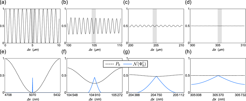
Figure 4: Probabilities $P_{0}$ (black, dashed) and the corresponding BLP-non-Markovianities $\mathcal{N}(\Phi_{0}^{t})$ (blue, solid) as functions of the path difference $\Delta x$. The panels (e)–(h) are magnifications of the panels (a)–(d), respectively, where the magnified regions have been indicated with shading. $\mu=c/(780\text{ nm})$, $\sigma=5.68\times 10^{11}\text{ Hz}$, and $\Delta n=0.009$.

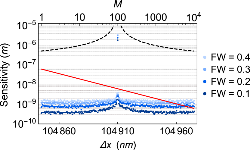
Figure 5: Sensitivity of $P_{0}$ (black, dashed) and $\mathcal{N}(\Phi_{0}^{t})$ (blue dots) with respect to $\Delta x$. Different shades of blue represent different widths of simulated noise. The red, solid line is the QCRB ($\approx$ 62 nm/$\sqrt{M}$). The sensitivities do not depend on $M$, and the QCRB does not depend on $\Delta x$. $\mu=c/(780\text{ nm})$, $\sigma=5.68\times 10^{11}\text{ Hz}$, and $\Delta n=0.009$.

At each value of $\Delta x$, we simulate additional noise (e.g. dark counts, background photons, and imperfections in the birefringent crystals) so that

$$\rho_{0}(t)=\Phi_{0}^{t}\big{(}\rho(0)\big{)}+\begin{pmatrix}\epsilon_{1}(t)&\epsilon_{2}(t)e^{i\epsilon_{3}(t)}\\ \epsilon_{2}(t)e^{-i\epsilon_{3}(t)}&-\epsilon_{1}(t)\end{pmatrix},$$ (14)

where $\epsilon_{1}(t)$ and $\epsilon_{2}(t)$ are drawn from a normal distribution with mean 0 and standard deviation $\tilde{\sigma}$, and the random phase $\epsilon_{3}(t)$ is drawn from a uniform distribution from 0 to $2\pi$. At each time step from 0 to coherence time, we draw separate noise terms for the initial states $|+\rangle$ and $|-\rangle$—redrawing them if the resulting state is nonphysical. Once the whole trace distance dynamics is fixed, we fit $|\kappa_{0}(t)|$ on it and evaluate $\tilde{\mathcal{N}}(\Phi_{0}^{t})$.

In Fig. 5, we have plotted the simulated sensitivities of memory effects (blue dots) with four different full widths (FW=$6\tilde{\sigma}$) of the additional random noise. The time steps, ranging from $2\pi\sigma\Delta nt_{min}=0$ to $2\pi\sigma\Delta nt_{max}=5$, were of the width $2\pi\sigma\Delta n\Delta t=0.01$. At each value of $\Delta x$, the algorithm was repeated 100 times to obtain $\Delta\mathcal{N}(\Phi_{0}^{t})$. The black, dashed curve in Fig. 5 is the sensitivity of $P_{0}$ with the observable used in Eq. (3) being $\mathds{1}\otimes\mathds{1}\otimes|0\rangle\langle 0|$. The red, solid line is the QCRB, calculated using Eqs. (4) and (5) and the state to which the phase difference is imprinted, $\frac{1}{\sqrt{2}}\int dfg(f)\big{(}e^{i2\pi fx_{0}/c}|f\rangle\otimes|0\rangle+e^{i2\pi fx_{1}/c}|f\rangle\otimes|1\rangle\big{)}$; When evaluating the QCRB, the measurement stage can be disregarded sensitivity . With our parameter choices, QCRB $\approx$ 62 nm/$\sqrt{M}$.

With a small number of measurements, the memory effects beat the QCRB by a few orders of magnitude. And even with more noise and measurements, when Eq. (4) is satisfied, the memory effects are clearly much more sensitive than the corresponding path probabilities that never reach the bound. Fig. 5 corresponds to Fig. 4(f), where $P_{0}>0.27$, meaning that the protocol does not suffer too much from losses.

Recent advancements in ultra-sensitive parameter estimation are based on parameter-dependent measurements beyond_1 —overlooked by the quantum Cramér-Rao theorem—and our protocol falls into this category, too. Our protocol depends on $\Delta x$ in the sense that, to fully capture the memory effects (or their absence), the process tomography needs to extend until $t\approx\frac{|\Delta x|}{c|\Delta n|}$. However, the conflict with the quantum Cramér-Rao theorem may be resolved in even simpler terms. While the usual parameter estimation framework is based on measurements on some probe state, we are interested in channels generated by $\Delta x$. Like parameter-dependent measurements, the global properties of channels are not considered by the quantum Cramér-Rao theorem.

V Conclusions and discussion

In this work, we have introduced an alternative source of non-Markovianity in the linear optical framework and analyzed its sensitivity with respect to the memory-inducing parameter, namely, the path difference of an unbalanced Mach-Zehnder interferometer. The path difference entangles two subenvironments (frequency and path) with each other, after which the open-system (polarization) dynamics is described by a Markovian convex combination of two CPTP maps that can be either Markovian or non-Markovian. Post-selecting only one of the maps and measuring its BLP-non-Markovianity allows us to probe the path difference (and hence, the concurrence of the frequency-path state) with high accuracy.

Numerical analysis implies that the sensitivity of memory effects can not only beat that of the corresponding path probability but the QCRB itself—proving decoherence and non-Markovianity as useful resources. We are able to break the QCRB, because we go beyond the standard parameter estimation scheme where one extracts information on parameter $\lambda$ by measurements on state $\rho$. Instead, we focus on the global properties of the channel $\Phi_{j}^{t}$. This raises an important question for future research: What is the corresponding precision limit for quantum processes? Previous works related to noisy parameter estimation have treated channels as snapshots of the open-system dynamics, giving interaction time dependent bounds dyn_qcrb_1 ; dyn_qcrb_2 ; dyn_qcrb_3 , but here we mean the overarching dynamics. In the case of this paper, such a limit would effectively rule out certain bandwidths of random noise.

Although our results have exciting implications on parameter estimation, the protocol also has its shortcomings. With small path differences the memory effects—though extremely sensitive—become less probable to appear, and if they do, the photon counts are equally low. Still, as our results highlight the great flexibility of open system interferometers, an optimal parameter estimation protocol might combine more traditional methods with ours.

References

- (1) H.-P. Breuer and F. Petruccione, The Theory of Open Quantum Systems (Oxford University Press, Oxford, 2007).
- (2) Á. Rivas, S. F. Huelga, and M. B. Plenio, Rep. Prog. Phys. 77, 094001 (2014).
- (3) H.-P. Breuer, E.-M. Laine, J. Piilo, and B. Vacchini, Rev. Mod. Phys. 88, 021002 (2016).
- (4) I. de Vega and D. Alonso, Rev. Mod. Phys. 89, 015001 (2017).
- (5) L. Li, M. J. W. Hall, and H. M. Wiseman, Phys. Rep. 759, 1 (2018).
- (6) C.-F. Li, G.-C. Guo, and J. Piilo, Europhys. Lett. 127, 50001 (2019).
- (7) C.-F. Li, G.-C. Guo, and J. Piilo, Europhys. Lett. 128, 30001 (2019).
- (8) Y. Dong, Y. Zheng, S. Li, C.-C. Li, X.-D. Chen, G.-C. Guo, and F.-W. Sun, npj Quantum Inf. 4, 3 (2018).
- (9) E.-M. Laine, H.-P. Breuer, and J. Piilo, Sci. Rep. 4, 4620 (2014).
- (10) Z.-D. Liu, Y.-N. Sun, B.-H. Liu, C.-F. Li, G.-C. Guo, S. Hamedani Raja, H. Lyyra, and J. Piilo, Phys. Rev. A 102, 062208 (2020).
- (11) S. Utagi, R. Srikanth, and S. Banerjee, Quantum Inf. Process. 19, 366 (2020).
- (12) P. Kwiat, A. Berglund, J. Altepeter, and A. White, Science 290, 498 (2000).
- (13) J.-S. Xu, X.-Y. Xu, C.-F. Li, C.-J. Zhang, X.-B. Zou, and G.-C. Guo, Nat. Commun. 1, 7 (2010).
- (14) A. Shaham and H. S. Eisenberg, Phys. Rev. A 83, 022303 (2011).
- (15) B.-H. Liu, L. Li, Y.-F. Huang, C.-F. Li, G.-C. Guo, E.-M. Laine, H.-P. Breuer, and J. Piilo, Nat. Phys. 7, 931 (2011).
- (16) A. Shaham and H. S. Eisenberg, Opt. Lett. 37, 2643 (2012).
- (17) E.-M. Laine, H.-P. Breuer, J. Piilo, C.-F. Li, and G.-C. Guo, Phys. Rev. Lett. 108, 210402 (2012); 111, 229901(E) (2013).
- (18) Z.-D. Liu, H. Lyyra, Y.-N. Sun, B.-H. Liu, C.-F. Li, G.-C. Guo, S. Maniscalco, and J. Piilo, Nat. Commun. 9, 3453 (2018).
- (19) S. Hamedani Raja, K. P. Athulya, A. Shaji, and J. Piilo, Phys. Rev. A 101, 042127 (2020).
- (20) G. M. Palma, K.-A. Suominen, and A. Ekert, Proc. R. Soc. A 452, 567 (1996).
- (21) O. Siltanen, T. Kuusela, and J. Piilo, Phys. Rev. A 103, 032223 (2021).
- (22) O. Siltanen, T. Kuusela, and J. Piilo, Phys. Rev. A 104, 042201 (2021).
- (23) J.-D. Lin, C.-Y. Huang, N. Lambert, G.-Y. Chen, F. Nori, and Y.-N. Chen, Phys. Rev. Res. 4, 033143 (2022).
- (24) S. Lorenzo, F. Plastina, and M. Paternostro, Phys. Rev. A 84, 032124 (2011).
- (25) D. Xie and A. M. Wang, Int. J. Quantum Inf. 13, 1550040 (2015).
- (26) C. Helstrom, Phys. Lett. A 25, 101 (1967).
- (27) L. Seveso, M. A. C. Rossi, and M. G. A. Paris, Phys. Rev. A 95, 012111 (2017).
- (28) F. Piacentini et al., Nat. Phys. 13, 1191 (2017).
- (29) D.-J. Zhang and J. Gong, Phys. Rev. Res. 2, 023418 (2020).
- (30) L. Seveso and M. G. A. Paris, Int. J. Quantum Inf. 18, 2030001 (2020).
- (31) E. Rebufello et al., Appl. Sci. 11, 4260 (2021).
- (32) M. Nielsen and I. Chuang, Quantum Computation and Quantum Information (Cambridge University Press, Cambridge, 2000).
- (33) H.-P. Breuer, E.-M. Laine, and J. Piilo, Phys. Rev. Lett. 103, 210401 (2009).
- (34) J. Teittinen, H. Lyyra, B. Sokolov, and S. Maniscalco, New J. Phys. 20, 073012 (2018).
- (35) S. Milz, M. S. Kim, F. A. Pollock, and K. Modi, Phys. Rev. Lett. 123, 040401 (2019).
- (36) A. A. Budini, Phys. Rev. Lett. 121, 240401 (2018).
- (37) S. Ataman, A. Preda, and R. Ionicioiu, Phys. Rev. A 98, 043856 (2018).
- (38) M. G. A. Paris, Int. J. Quantum Inf. 7, 125 (2009).
- (39) B. M. Escher, R. L. de Matos Filho, and L. Davidovich, Nat. Phys. 7, 406 (2011).
- (40) S. Alipour, M. Mehboudi, and A. T. Rezakhani, Phys. Rev. Lett. 112, 120405 (2014).
- (41) N. Mirkin, M. Larocca, and D. Wisniacki, Phys. Rev. A 102, 022618 (2020).
- (42) P. Rungta, V. Bužek, C. M. Caves, M. Hillery, and G. J. Milburn, Phys. Rev. A 64, 042315 (2001).