ViTALiTy: Unifying Low-rank and Sparse Approximation for Vision Transformer Acceleration with a Linear Taylor Attention

Abstract

Vision Transformer (ViT) has emerged as a competitive alternative to convolutional neural networks for various computer vision applications. Specifically, ViTs’ multi-head attention layers make it possible to embed information globally across the overall image. Nevertheless, computing and storing such attention matrices incurs a quadratic cost dependency on the number of patches, limiting its achievable efficiency and scalability and prohibiting more extensive real-world ViT applications on resource-constrained devices. Sparse attention has been shown to be a promising direction for improving hardware acceleration efficiency for NLP models. However, a systematic counterpart approach is still missing for accelerating ViT models. To close the above gap, we propose a first-of-its-kind algorithm-hardware codesigned framework, dubbed ViTALiTy, for boosting the inference efficiency of ViTs. Unlike sparsity-based Transformer accelerators for NLP, ViTALiTy unifies both low-rank and sparse components of the attention in ViTs. At the algorithm level, we approximate the dot-product softmax operation via first-order Taylor attention with row-mean centering as the low-rank component to linearize the cost of attention blocks and further boost the accuracy by incorporating a sparsity-based regularization. At the hardware level, we develop a dedicated accelerator to better leverage the resulting workload and pipeline from ViTALiTy’s linear Taylor attention which requires the execution of only the low-rank component, to further boost the hardware efficiency. Extensive experiments and ablation studies validate that ViTALiTy offers boosted end-to-end efficiency (e.g., $3\times$ faster and $3\times$ energy-efficient) under comparable accuracy, with respect to the state-of-the-art solution.

I Introduction

Vision Transformers (ViT) are gaining increasing popularity with their state-of-the-art performance in various computer vision tasks [16, 38, 23, 20, 26, 44]. Compared to Convolutional Neural Networks (CNNs) which exploit local information through convolutional layers, ViT uses multi-head attention (MHA) modules to capture global information and long-range interactions, showing superior accuracy against CNNs [16]. Nevertheless, computing and storing such attention matrices incurs a quadratic computational and memory cost dependency on the number of patches (input resolution).

To better understand the runtime breakdown for ViTs’ MHA module, we profile DeiT-Tiny [38], a popular ViT model, on various commercial devices, such as NVIDIA RTX 2080Ti [32], NVIDIA Edge GPU TX2 [31], and Google Pixel3 phone [19]. In Fig.  1, we observe that computing the softmax attention (Step 2) consistently dominates ($52\%-58\%$) the MHA runtime, especially when devices become less powerful and more resource-constrained. Hence, the major bottleneck for ViTs is the softmax attention, which limits their achievable efficiency and scalability, and prohibits extensive real-world ViT applications on resource-constrained devices.

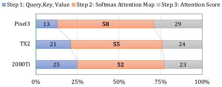
Figure 1: Runtime breakdown of DeiT-Tiny MHA on various devices.

To alleviate the above quadratic complexity, a simple approach is to reduce the number of patches or input resolution. However, this would result in larger patch sizes with an additional burden on hardware resources to compute the corresponding queries, keys, and values (Step 1 in Fig. 1). Moreover, many real-world computer vision applications, such as medical imaging, autonomous driving, drone imagery and surveillance, etc, require high resolution inputs to discover finer-grained details in the images [4].

A popular alternative approach in Transformers for Natural Language Processing (NLP) is to use sparse attention. Here, the attention matrix generated by the dot product between the dense queries and keys is made sparse by using a binary mask. Then, the sparse attention matrix with reduced entries goes through the softmax operation after which it is multiplied by a dense value matrix. Many works in algorithm [2, 10, 48, 12, 13, 49] and hardware [21, 40, 28, 33, 22] have been proposed to implement such sparse attentions for NLP-based Transformer models by efficiently tackling various static and dynamic sparse patterns.

Orthogonal to the aforementioned techniques, we replace the vanilla softmax attention with a linear attention, and leverage the matrix associative property to linearize the cost of computing ViTs’ attentions. Such linear attention has been proposed for NLP-based Transformer models [24, 11]. However, there is a missed opportunity in applying linear attentions to ViTs. Unlike sparsity-based accelerators, we seek to exploit the low-rank property of the proposed linear attention to design dedicated accelerator for improved latency and energy efficiency. Our main contributions are summarized below:

1. We propose an algorithm-accelerator codesign framework, dubbed ViTALiTy, that unifies low-rank and sparse approximation to boost the achievable accuracy-efficiency of ViTs using linear Taylor attentions. To the best of our knowledge, this is first of its kind work dedicated for ViTs by exploiting the low-rank properties in linear attentions.

2. On the algorithm level, we propose a linear attention for reducing the computational and memory cost by decoupling the vanilla softmax attention into its corresponding “weak” and “strong” Taylor attention maps. Unlike the vanilla attentions, the linear attention in ViTALiTy generates a global context matrix $\mathbf{G}$ by multiplying the keys with the values. Then, we unify the low-rank property of the linear attention with a sparse approximation of “strong” attention for training the ViT model. Here, the low-rank component of our ViTALiTy attention captures global information with a linear complexity, while the sparse component boosts the accuracy of linear attention model by enhancing its local feature extraction capacity.

3. At the hardware level, we develop a dedicated accelerator to better leverage the algorithmic properties of ViTALiTy’s linear attention, where only a low-rank component is executed during inference favoring hardware efficiency. Specifically, ViTALiTy’s accelerator features a chunk-based design integrating both a systolic array tailored for matrix multiplications and pre/post-processors customized for ViTALiTy attentions’ pre/post-processing steps. Furthermore, we adopt an intra-layer pipeline design to leverage the intra-layer data dependency for enhancing the overall throughput, together with a down-forward accumulation dataflow for the systolic array to improve hardware efficiency.

4. We perform extensive experiments and ablation studies to demonstrate the effectiveness of ViTALiTy in terms of latency speedup ($3\times$), and energy efficiency ($3\times$) under comparable model accuracy with respect to the state-of-the-art solution.

II Background and Motivation

II-A Preliminaries of Vision Transformers

ViT Model Architecture. Fig. 2 illustrates the model architecture for ViTs. Here, each input image is divided and arranged into a sequence of patches (or tokens), which are then fed into an $L$-layer Transformer encoder [39]. Each Transformer layer comprises a multi-head attention (MHA) module and a multi-layer perceptron (MLP) module. As an example, the DeiT-Tiny model [38] consists of $L=12$ Transformer layers where the typical input image resolution is $224\times 224$ with patch size $16\times 16$; This results in a sequence of $n=196$ patches (tokens) with each token embedded as $64\times 3$ with $h=3$ heads, and $d=64$ dimensions per head.

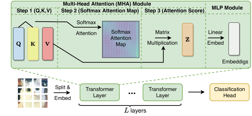
Figure 2: Each Transformer layer in a ViT model comprises a Multi-Head Attention (MHA) module and a Multi-Layer Perceptron (MLP) module.

Attentions in ViTs. The MHA module enables ViTs’ impressive success in various tasks by enhancing the model’s capacity to capture global information as compared to CNNs. Specifically, MHA receives $\mathbf{X}\in\mathbb{R}^{n\times d}$ as its input and outputs $\mathbf{Z}\in\mathbb{R}^{n\times d}$ as the attention score, which involves the following three computational steps as shown in Fig.  2.

Step 1: Compute the query, key, value vectors

$$\mathbf{Q}=\mathbf{X}\mathbf{W}^{Q},\mathbf{K}=\mathbf{X}\mathbf{W}^{K},\mathbf{V}=\mathbf{X}\mathbf{W}^{V},$$

where $\mathbf{Q}$, $\mathbf{K}$, $\mathbf{V}\in\mathbb{R}^{n\times d}$ are the input embeddings for the next step. $\mathbf{W}^{Q},\mathbf{W}^{K},\mathbf{W}^{V}\in\mathbb{R}^{d\times d}$ are learned weights.

Step 2: Compute the softmax attention map

$$\mathbf{S}=\texttt{softmax}\Big{(}\frac{\mathbf{Q}\mathbf{K}^{T}}{\sqrt{d}}\Big{)}$$

Step 3: Compute the attention score, $\mathbf{Z}=\mathbf{S}\mathbf{V}$

Before moving to the next layer, the attention scores are sent to the MLP module, $\mathbf{O}=\mathbf{Z}\mathbf{W}^{O},\text{where, }\mathbf{W}^{O}\in\mathbb{R}^{d\times d}$.

II-B Related Work

Efficient Vision Transformers. Motivated by the breakthroughs of Transformers [39, 15, 34, 26] in NLP, there has been a growing interest in developing Transformers for vision tasks. ViT [16] was the first to show that Transformers can completely replace convolutions by treating images as a sequence of patches of fixed length. Since then, ViT models and their variants have been successfully used for image recognition [16, 38], object detection [5, 51], and segmentation [46]. To capture fine-grained spatial details of different scales, multi-stage hierarchical ViTs, such as Pyramid ViT [42], Swin Transformer [26], Focal Transformer [45], and CrossViT [7], have been proposed, where the number of tokens is gradually reduced while the token feature dimension is progressively increased. Recent works in deploying efficient ViTs have sparked great interest. For example, by replacing local processing in convolutions with global processing via attention, MobileViT [30] strives to combine the strengths of CNNs and ViTs; LeViT [20] adopts a hybrid neural architecture. In parallel, compact ViT models via pruning [50] have been developed by encouraging dimension-wise sparsity; [27] proposes a post-training mixed-precision quantization scheme for reducing ViTs’ memory storage and computational costs; and neural architecture search (NAS) has been adopted to discover better ViT models, e.g., NASViT [18] is derived from Supernet-based one-shot NAS.

Linear Attentions. To alleviate the quadratic complexity associated with computing and storing attentions in Transformers, linear attention [24, 11, 36] replaces the softmax operation with a generic similarity function defined as $\texttt{sim}(\mathbf{Q},\mathbf{K})=\phi(\mathbf{Q})\phi(\mathbf{K})^{T}$, where $\phi()$ is a kernel or low-rank function. The above formulation exploits the matrix associative property to compute $\phi(\mathbf{Q})\big{(}\phi(\mathbf{K})^{T}\mathbf{V}\big{)}$, thereby reducing the quadratic computational complexity in vanilla Transformer attentions to a linear one. For NLP, Linear Transformer [24] defines a kernel function $\phi()=\texttt{elu}()+1$, while Performer [11] uses positive orthogonal random features (PORF) as a low-rank function $\phi()$. Scatterbrain [6] shows that combining both low-rank (via kernel feature map in Performer [11]) linear attention, and sparse attention (via locality sensitive hashing in Reformer [25]) leads to efficient approximation with better performance than the individual components. For vision tasks, Efficient Attention [36] uses $\phi()=\texttt{softmax}()$ separately on queries and keys to approximate the vanilla softmax attentions.

Transformer Accelerators. There has been a surge in software-hardware co-designed accelerators dedicated to NLP Transformers which leverage dynamic sparsity patterns to tackle the quadratic complexity in storing and computing the attentions, e.g., $A^{3}$ [21], SpAtten [40], Sanger [29], ELSA [22], and DOTA [33]. Specifically, $A^{3}$ [21] greedily searches for key vectors which are most relevant to the current query vector for approximating the vanilla attentions, but can suffer from low speedup and poor accuracy under high sparsity ratios; SpAtten [40] attempts to remove attention heads and tokens via structured pruning, which may still contain redundant attentions, leading to a low achievable sparsity; Sanger [29] dynamically sparsifies the vanilla attentions based on a quantized prediction of the attentions followed by rearranging the sparse mask via a “pack and split” strategy into hardware-friendly structured blocks; ELSA [22] adopts binary hashing maps to estimate the angles between the queries and keys for approximating attentions, for enabling lightweight similarity computation together with a specialized accelerator, which can suffer from a degraded accuracy; and DOTA [33] adopts both low precision and low-rank linear transformation to predict the sparse attention masks by jointly optimizing a lightweight detector together with the Transformer to accurately detect and omit weak connections during runtime.

II-C Gaps and Opportunities

In contrast to existing dynamic sparsity-based accelerators dedicated to NLP Transformers, there still exists a missing gap for ViT accelerators. Unlike NLP Transformers and their corresponding accelerators which deal with input sequences of varying lengths during runtime, ViTs only needs to handle a fixed-length input sequence (tokens) of image patches. Hence, there is an opportunity to leverage this unique property to boost the efficiency of ViT acceleration.

Overall, existing works on efficient ViT models focus on the model architectures, while existing Transformer accelerators target sparse attentions of NLP Transformers. Hence, a systematic counterpart approach is still missing for accelerating ViT models. Moreover, there is still a lack of works exploiting low-rank properties of attentions for designing ViT accelerators with boosted hardware efficiency. Finally, there is a great potential of training ViT models with combination of low-rank linear attentions and sparse attentions for restoring the accuracy of linear attention ViTs. To close the above gaps, we propose a first-of-its-kind algorithm-hardware co-designed framework dedicated to ViT inference via linear Taylor attentions. Unlike the Scatterbrain [6] algorithm, we decouple vanilla softmax attentions as a combination of low-rank and sparse approximations during training to boost the accuracy of linear attention ViTs, and drop the sparse attention while retaining the linear attention during inference to avoid any run-time overhead associated with dynamic sparse attentions.

III Proposed ViTALiTy Algorithm

III-A Distribution of ViT Attentions

Here we first analyze the distribution of ViT attention values under row-wise mean-centering, and then present a motivating observation for our proposed ViTALiTy algorithm. To do so, we begin by reviewing a key property of softmax functions with mean-centered input sequences.

Property 1 (Mean-Centering).

Given a sequence of $n$ data samples denoted as $\mathbf{x}=\{x_{i},\;i=1,\ldots,n\}$ with a scalar mean $\overline{x}$, it can be analytically shown that subtracting a scalar value does not change the softmax output.

$$\texttt{softmax}(\mathbf{x}-\overline{x})_{i}=\frac{\texttt{exp}({x_{i}-\overline{x})}}{\sum_{i=1}^{n}\texttt{exp}({x_{i}-\overline{x})}}=\texttt{softmax}(\mathbf{x})_{i}$$

We seek to apply the above property to the scaled dot product attention (similarity) matrix, $\frac{\mathbf{QK^{T}}}{\sqrt{d}}$, as the input to the softmax function. However, computing row-wise mean-centering of the dot product attention matrix for each head is computationally expensive, as it relies on first computing, and storing the attention which is quadratic in $n$.

Proposed Efficient Mean-Centering Attentions. To alleviate the above challenge for all rows $i\in[n]$, we propose to efficiently compute the mean-centering rows of the attention in linear time by directly modifying the key matrix, $\mathbf{K}$.

$$\frac{\mathbf{QK^{T}}}{\sqrt{d}}-\;\texttt{mean}\bigg{(}\frac{\mathbf{QK^{T}}}{\sqrt{d}}\bigg{)}=\frac{\mathbf{Q}}{\sqrt{d}}\big{(}\mathbf{K}-\mathbf{1}_{n}\overline{\mathbf{K}}\big{)}^{T}=\frac{\mathbf{Q}\hat{\mathbf{K}}^{T}}{\sqrt{d}},$$

$$\text{where, }\overline{\mathbf{K}}=\frac{1}{n}\sum_{j=1}^{n}\mathbf{k}_{j}=\frac{1}{n}\big{(}\mathbf{1}_{n}^{T}\mathbf{K}\big{)}$$

$\hat{\mathbf{K}}$ is the mean-centered key matrix that allows us to avoid computing, and storing the more expensive $\mathbf{QK^{T}}$ attention for each head prior to performing mean-centering. The key benefit of mean-centering is to regularize the softmax inputs to be centered around zero so that their distribution is geared towards a normal distribution curve for a majority number of inputs (Central Limit Theorem), thereby ensuring that more samples fall within the interval $[-1,1)$. By leveraging Property 1 for each row of an attention matrix, we get

$$\texttt{softmax}\bigg{(}\frac{\mathbf{Q}\hat{\mathbf{K}}^{T}}{\sqrt{d}}\bigg{)}=\texttt{softmax}\bigg{(}\frac{\mathbf{QK^{T}}}{\sqrt{d}}\bigg{)},$$

which transforms the similarity between the queries and modified keys, $(\mathbf{q}_{i}\hat{\mathbf{k}}_{j}^{T})$, to be centered around zero-mean without changing the softmax outputs.

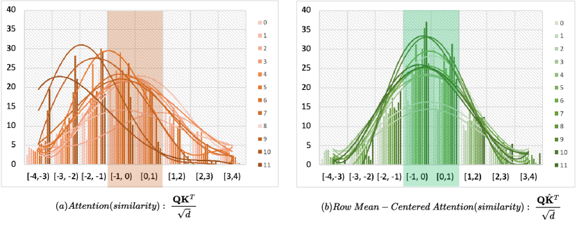
Figure 3: Distribution of attentions (inputs to softmax) across various layers 0-11: (a) the vanilla attention distribution shifts left, and (b) row-wise mean-centering of attentions centers the distribution towards [-1,1). Here we use the DeiT-Tiny [38] model on the ImageNet dataset as an example.

Motivating Observation. Fig. 3 visualizes the distribution of attention (similarity) matrices of various layers in the DeiT-Tiny ViT model with multiple heads on the ImageNet dataset, before and after mean-centering. We observe that up to $67\%$ entries of the mean-centered attention values lie within the interval $[-1,1)$ compared with that of $46\%$ in the vanilla ones, i.e., 21% increase after mean-centering. In other words, efficiently row-wise mean-centering the attentions centers majority of the similarity between the queries and modified keys around zero, thereby revealing denser weak connections. Furthermore, the similarity values lying outside the interval $[-1,1)$ are sparser in quantity but represent stronger connections between queries and keys. This motivates that the mean-centered softmax attention can be decoupled into a sum of “weak” and “strong” attentions which is realized by the proposed Taylor attention.

III-B Constructing Taylor Attentions for ViTs

We define Taylor attention based on Taylor series expansion of the exponential function $\texttt{exp}()$ used in row-wise mean-centered softmax attention. We recall that up to $67\%$ of the similarity matrix lies within the interval $[-1,1)$ representing denser weak connections. Since Taylor series approximation for values close to zero can be represented with first-order Taylor expansion, we get $\texttt{exp}(\mathbf{q}_{i}\hat{\mathbf{k}}_{j}^{T})\approx 1+\mathbf{q}_{i}\hat{\mathbf{k}}_{j}^{T}$. However, a key challenge here is to accurately locate the weak (query, key) connections within the attention matrix for a given input. In concurrent work for NLP-based Transformer accelerators  [40, 33, 22, 29], these weak connections are dynamically computed or predicted during runtime which are pruned resulting in irregular sparse attention patterns and complex designs for the corresponding accelerator. In contrast, for ViTs our novelty lies in decoupling the softmax attentions as a combination of “weak” and “strong” Taylor attention maps without any overheads of identifying the weak connections and generating dynamic sparse attention patterns during runtime.

The “weak” Taylor attention map is computed by the first-order ($m=1$) Taylor approximation of the original softmax attention matrix capturing the weak connections between $\mathbf{Q}$ and $\hat{\mathbf{K}}$. Let, $\hat{\mathbf{k}}_{sum}=\sum_{j=1}^{n}\hat{\mathbf{k}}_{j}=\mathbf{1}_{n}^{T}\hat{\mathbf{K}}$.

$$\scriptsize{\texttt{Taylor}_{softmax}\bigg{(}\frac{\mathbf{Q}\hat{\mathbf{K}}^{T}}{\sqrt{d}}\bigg{)}\Bigg{|}_{m=1}=\Bigg{[}\texttt{Taylor}_{softmax}\bigg{(}\frac{\mathbf{q}_{i}\hat{\mathbf{K}}^{T}}{\sqrt{d}}\bigg{)}\Bigg{]}_{i\in[n]}}$$

$$=\texttt{diag}^{-1}\big{(}n\sqrt{d}\mathbf{1}_{n}+\mathbf{Q}\hat{\mathbf{k}}_{sum}^{T}\big{)}\times\Big{(}\sqrt{d}\;\mathbf{1}_{n}\mathbf{1}_{n}^{T}+\mathbf{Q}\hat{\mathbf{K}}^{T}\Big{)}$$

However, directly replacing a softmax attention with the first-order Taylor attention in a pre-trained ViT models leads to poor accuracy, which we further validate in Fig. 10 (LowRank). This degradation in accuracy is explained by incorrectly assuming that all (query, key) connections are weak with their similarity measure falling within the interval $[-1,1)$, for various layers and heads across different inputs in a ViT model. Hence, it is imperative to include the corresponding higher-order ($m>1$) terms from the Taylor series expansion of $\texttt{exp}\big{(}\frac{\mathbf{Q}\hat{\mathbf{K}}^{T}}{\sqrt{d}}\big{)}$ to compensate for the (query, key) pairs with similarity outside the interval $[-1,1)$ representing “strong” connections by their magnitude. Hence, we decouple the vanilla softmax attention as follows:

$$\texttt{softmax}\bigg{(}\frac{\mathbf{Q}\mathbf{K}^{T}}{\sqrt{d}}\bigg{)}=\texttt{softmax}\bigg{(}\frac{\mathbf{Q}\hat{\mathbf{K}}^{T}}{\sqrt{d}}\bigg{)}$$

$$\small{\approx\underbrace{\texttt{Taylor}_{softmax}\bigg{(}\frac{\mathbf{Q}\hat{\mathbf{K}}^{T}}{\sqrt{d}}\bigg{)}\Bigg{|}_{m=1}}_{\text{"weak attention"}}+\underbrace{\texttt{Taylor}_{softmax}\bigg{(}\frac{\mathbf{Q}\hat{\mathbf{K}}^{T}}{\sqrt{d}}\bigg{)}\Bigg{|}_{m>1}}_{\text{"strong attention"}}}$$

III-C Taylor Attention is a Double-edged Sword

Representing the vanilla softmax attention as a combination of “weak” and “strong” Taylor attention maps has both advantages and disadvantages which we discuss below.

Advantages. ① The “weak” Taylor attention represents a linear attention which enables exploiting the associative property of matrix multiplication for enabling a linear computational and memory complexity with the number of patches/tokens. Putting aside the normalization, the “weak” Taylor attention switches the order of the softmax attention from $\big{(}\mathbf{Q}\hat{\mathbf{K}}^{T}\big{)}\mathbf{V}$ to more-efficient $\mathbf{Q}\big{(}\hat{\mathbf{K}}^{T}\mathbf{V}\big{)}$. Though the final attention output dimension $n\times d$ remains the same, the computational time complexity reduces from quadratic $\mathbfcal{O}(n^{2}d)$ to linear $\mathbfcal{O}(nd^{2})$. Consequently, there is no need to compute and store the $\mathbfcal{O}(n^{2})$ attention matrix $\big{(}\mathbf{Q}\hat{\mathbf{K}}^{T}\big{)}$ for each query, rather a global context matrix, $\mathbf{G}=\big{(}\hat{\mathbf{K}}^{T}\mathbf{V}\big{)}$ is computed and stored with a memory cost of $\mathbfcal{O}(d^{2})$, which is independent of the number of patches. Therefore, a linear Taylor attention can lead to both 1) a lower complexity and 2) a higher hardware utilization thanks to its resulting dense linear attention matrix.

② Linear attention can enhance our understanding of softmax attentions via low-rank Taylor attention maps capturing various global contextual information. Here the global context matrix $\mathbf{G}$ can be interpreted as a collection of distinct semantic aspects of the input aggregated by their corresponding values, i.e., different rows $\mathbf{g}_{i}$ correspond to a summary of distinct global context vectors that capture the foreground, core object, periphery, etc. This leads to enhanced understanding that the low-rank matrix, $\mathbf{QG}$ in the proposed (un-normalized) Taylor attention, $\sqrt{d}\big{(}\mathbf{1}_{n}\mathbf{v}_{sum}\big{)}+\mathbf{Q}\mathbf{G}$, is a linear combination, for which the weights are a set of coefficients in each query, of a set of global template attention maps, each having a semantically significant focus. In other words, pixels belonging to a particular semantic group might contribute a larger weighted coefficient to its corresponding global context vector in the linear attention, resulting in much refined score [36]. Moreover, $\sqrt{d}\big{(}\mathbf{1}_{n}\mathbf{v}_{sum}\big{)}$ is a rank-$1$ matrix and independent of the query and may represent the background attention.

Disadvantages. A key challenge in Taylor attention is computing the “strong” attention which represents the higher-order terms $m>1$ of Taylor expansion. Firstly, computing the optimal Taylor order for given input is non-trivial. Secondly, generating the higher-order Taylor attention maps requires multiplying the complete query and key matrices together for various orders which has quadratic complexity thereby eclipsing the advantages of linear attention. Therefore, we seek to estimate the “strong” attention based on sparse approximation.

Figure 4: ViTALiTY workflow comprising the proposed (Low-Rank) Linear Taylor attention (order, $m=1$): (i) Higher-order Taylor terms ($m>1$) when added results in vanilla softmax attention score, (ii) Training phase (unifying low-rank and sparse approximation) where higher-order Taylor terms are approximated as Sparse attention (computed using Sanger [28]), and (iii) Inference phase that uses only the (Low-Rank) Linear Taylor attention.

III-D Proposed: Unifying Low-rank and Sparse Attentions

As discussed earlier, combining the “strong” Taylor attention helps boost the achievable accuracy of ViTs against using only the “weak” Taylor attention. While the “weak” Taylor attention being a linear attention captures only the global context without explicitly computing the attention matrix, it lacks the non-linear attention score normalization. Consequently, this weakens its ability to extract local features from high attention scores produced by local patterns in the input image resulting in degraded accuracy  [17, 8, 37, 4]. To enhance the local feature extraction capacity and boost the accuracy of linear attention ViTs, we seek to unify the above “weak” Taylor attention (dense low-rank) with the “strong” attention (sparse approximation) that captures the non-linear relationship between (queries, keys). In contrast to combining different works on low-rank and sparse components in Scatterbrain [6], ViTALiTy is unique as it decouples the vanilla softmax attention into the corresponding low-rank component given by the proposed linear Taylor attention, $\sqrt{d}\big{(}\mathbf{1}_{n}\mathbf{v}_{sum}\big{)}+\mathbf{Q}\mathbf{G}$, depicting global context, and the sparse component based on approximating the higher-order terms capturing the local features with “strong” connections as illustrated in Fig 4. We use the sparsity prediction mask generated by the quantized query and key following Sanger [28] for fine-tuning our models. Our key insights which we empirically validate in Section V-D are:

1. We show that the widely used softmax attention could represent both low-rank and sparse components. During training, the low-rank component, i.e., linear Taylor attention allows the sparse attention to exhibit more sparsity with higher thresholds while the sparse component helps boost the accuracy of otherwise low-rank Taylor attention model.

2. During inference, we discover that using only the low-rank component, i.e., linear Taylor attention is sufficient as it exhibits similar accuracy to that of combined low-rank and sparse attention. This reveals that the sparse component acts as a regularizer to help boost the accuracy of linear Taylor attention during training, and hence can be dropped during inference to avoid overhead of dynamic sparse attentions.

Input: $\mathbf{Q}$, $\mathbf{K}$, $\mathbf{V}$ are queries, keys, values

Output: $\mathbf{Z}$ is the Taylor attention score

$\triangleright$ Step 1: Mean-centering keys

 $\overline{\mathbf{K}}\leftarrow\frac{1}{n}\big{(}\mathbf{1}_{n}^{T}\mathbf{K}\big{)}$, cost:$\mathbfcal{O}(nd)$

 $\hat{\mathbf{K}}\leftarrow\mathbf{K}-\mathbf{1}_{n}\overline{\mathbf{K}}$, cost:$\mathbfcal{O}(nd)$

$\triangleright$ Step 2: Global context matrix

 $\mathbf{G}\leftarrow\hat{\mathbf{K}}^{T}\mathbf{V}$, cost:$\mathbfcal{O}(nd^{2})$

$\triangleright$ Step 3: Column sum of keys, values

 $\hat{\mathbf{k}}_{sum}\leftarrow\mathbf{1}_{n}^{T}\hat{\mathbf{K}}$, cost:$\mathbfcal{O}(nd)$

 $\mathbf{v}_{sum}\leftarrow\mathbf{1}_{n}^{T}\mathbf{V}$, cost:$\mathbfcal{O}(nd)$

$\triangleright$ Step 4: Compute Taylor denominator

 $\mathbf{t}_{D}\leftarrow\big{(}n\sqrt{d}\big{)}\mathbf{1}_{n}+\mathbf{Q}\hat{\mathbf{k}}_{sum}^{T}$, cost:$\mathbfcal{O}(nd)$

$\triangleright$ Step 5: Compute Taylor numerator

 $\mathbf{T}_{N}\leftarrow\sqrt{d}\big{(}\mathbf{1}_{n}\mathbf{v}_{sum}\big{)}+\mathbf{Q}\mathbf{G}$, cost:$\mathbfcal{O}(nd^{2})$

$\triangleright$ Step 6: Taylor attention score

 $\mathbf{Z}\leftarrow\texttt{diag}^{-1}\big{(}\mathbf{t}_{D}\big{)}\mathbf{T}_{N}$, cost:$\mathbfcal{O}(nd)$

Algorithm 1 ViTALiTy with Taylor Attention

Algorithm 1 presents the inference computational cost of ViTALiTy having a linear dependency on $n$, and Fig. 5 compares the computational workflow of the proposed Taylor attention score with that of the vanilla softmax attention score.

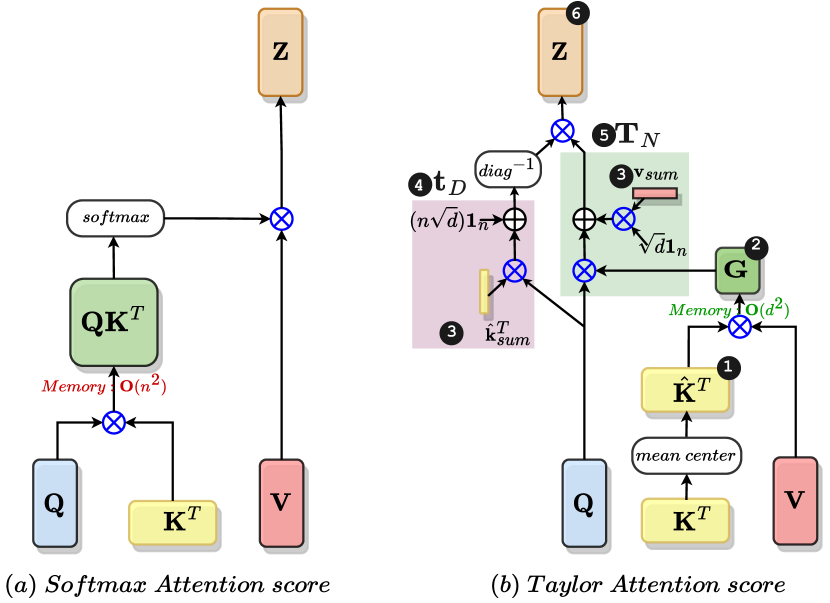
Figure 5: Computational steps (a) vanilla Softmax Attention and (b) our Taylor attention (see Algorithm 1), where the global context matrix $\mathbf{G}$ provides linear computation and memory benefits over the vanilla quadratic $\mathbf{Q}\mathbf{K}^{T}$.

IV Proposed ViTALiTy Accelerator

Here, we first analyze the computational complexity of the proposed Taylor attention, then discuss potential acceleration opportunities for leveraging our proposed attention, and finally present our developed ViTALiTy accelerator.

IV-A Complexity Analysis and Potential Opportunities

Theoretical Complexity Analysis. Here we discuss the theoretical complexity in terms of the ratios of operation numbers, $R$, between the vanilla softmax attention and the proposed Taylor attention. Recall, $n$ and $d$ denote the number of tokens and the feature dimensions. In Eqs. (1), (2), and (3), we compute the theoretical ratio of number, $R$, for multiplications (Mul.), additions (Add.), and divisions (Div.), respectively, and we conclude that: 1) In the vanilla softmax attention, the numbers of both multiplications (Mul.) (i.e., $\mathbf{QK}^{T}$ and $\mathbf{SV}$) and divisions (Div.) are nearly $(\mathbf{n}/\mathbf{d})\times$ more than those in our proposed Taylor attention (i.e., $\mathbf{G}=\hat{\mathbf{K}}^{T}\mathbf{V}$, $\mathbf{Q}\hat{\mathbf{k}}_{sum}^{T}$, and $\mathbf{Q}\mathbf{G}$ for Mul., and Steps 1 and 6 in Algorithm 1 for Div.); 2) While the number of addition (Add.) reduction in our Taylor attention compared to the vanilla attention is less than $(\mathbf{n}/\mathbf{d})\times$ owing to extra pre-processing steps (see Steps 1 and 3 in Algorithm 1); 3) Furthermore, in contrast to the vanilla attention, our Taylor attention does not have the computationally expensive exponentiation (Exp.).

$$\vspace{-0.5em}R_{Mul.}=\frac{2\times n\times n\times d}{(2\times n\times d\times d)+(n\times d)}=\frac{2n}{2d+1}\approx\frac{n}{d},$$ (1)

$$R_{Add.}=\frac{2\times n^{2}\times d+n^{2}}{(2\times n\times d^{2})+(7nd)}=\frac{(2d+1)n}{(2d+7)d}<\frac{n}{d},$$ (2)

$$R_{Div.}=\frac{n\times n}{nd+d}=\frac{n^{2}}{(n+1)d}\approx\frac{n}{d}.$$ (3)

TABLE I: Comparing operation numbers (M) between ViTALiTy Taylor attention and vanilla Softmax attention on ViT models.

	ViTALiTy			Baseline (vanilla softmax)
MODELS	Mul.	Add.	Div.	Mul.		Add.		Exp.	Div.
DeiT-Tiny	$58.3$	$61.0$	$0.5$	$178.8$	$(3.1\times)$	$180.2$	$(3.0\times)$	$1.4$	$1.4$	$(3.1\times)$
MobileViT-xs	$4.8$	$5.3$	$0.1$	$28.4$	$(5.9\times)$	$29.0$	$(5.5\times)$	$0.6$	$0.6$	$(5.1\times)$
LeViT-128	$3.4$	$4.0$	$0.1$	$36.4$	$(10.7\times)$	$37.5$	$(9.4\times)$	$1.1$	$1.1$	$(10.6\times)$

Table I empirically validates above conclusions, where we observe that for any given model, the ratios of numbers for each of the multiplications, additions, and division are nearly similar. Moreover, for various models, i.e., DeiT-Tiny [38], MobileViT-xs [30], and LeViT-128 [20], we find the ratio of operation numbers to be about $\textbf{3}\times$, $\textbf{5}\times$, and $\textbf{10}\times$, respectively.

Profiling Results Analysis. Despite the theoretical reduction of operation numbers in ViTALiTy’s Taylor attention as discussed above, existing general computing platforms or accelerators dedicated to the vanilla ViT’s attention cannot fully take advantage of our Taylor attention’s potential benefits to boost its achievable hardware efficiency. For example, Table II compares the profiling latency of both the proposed and vanilla attentions in several representative ViTs, including DeiT-Tiny [38], MobileViT-xs [30], and LeViT-128 [20] on a typical edge GPU (i.e., NVIDIA Tegra X2), and we can see that: 1) The softmax operation, which accounts for about $40\%$ of the overall latency, is arguably the dominant operator in the vanilla attention; 2) Although ViTALiTy adopts the Taylor attention to remove the hardware inefficient softmax operation and further reduce the number of multiplications/additions/divisions, its potential hardware efficiency does not reflect in the profiling latency on the GPU, motivating dedicated accelerators for our ViTALiTy algorithm; 3) As each step in Algorithm 1 is processed sequentially on the GPU without exploring potential pipeline opportunities, even the computationally light pre/post-processing steps contribute to a nontrivial amount of the overall latency.

TABLE II: The latency profiling results of ViTALiTy’s Taylor attention and the vanilla attention on the edge GPU (NVIDIA Tegra X2).

	DeiT-Tiny [38]		MobileViT-xs [30]		LeViT-128 [20]
ViTALiTy(Taylor attention)	Latency(ms)	Ratio	Latency(ms)	Ratio	Latency(ms)	Ratio
1: $\hat{\mathbf{K}}$	$1.40$	$10\%$	$0.41$	$15\%$	$0.65$	$15\%$
2: $\mathbf{G}$	$3.51$	$25\%$	$0.62$	$22\%$	$1.05$	$24\%$
3: $\mathbf{\hat{k}}_{sum}$, $\mathbf{v}_{sum}$	$1.40$	10%	$0.41$	$15\%$	$0.65$	$15\%$
4: $\mathbf{t}_{D}$	$2.24$	$16\%$	$0.41$	$15\%$	$0.65$	$15\%$
5: $\mathbf{T}_{N}$	$3.93$	$28\%$	$0.64$	$23\%$	$1.11$	$25\%$
6: $\mathbf{Z}$	$1.54$	$11\%$	$0.27$	$10\%$	$0.32$	$7\%$
OVERALL	14.03	$100\%$	2.76	100%	4.43	$100\%$
Baseline (vanilla softmax)	Latency(ms)	Ratio	Latency(ms)	Ratio	Latency(ms)	Ratio
1. $\mathbf{QK}^{T}$	$3.61$	$31\%$	$0.54$	$30\%$	$0.80$	$29\%$
2. $\mathbf{S}=\texttt{Softmax}(\mathbf{QK}^{T})$	$4.43$	$38\%$	$0.72$	$40\%$	$1.16$	$42\%$
3. $\mathbf{SV}$	$3.61$	$31\%$	$0.54$	$30\%$	$0.80$	$29\%$
OVERALL	11.65	100%	1.79	$100\%$	2.76	$100\%$

Based on the theoretical and profiling analysis above, we next discuss potential opportunities of leveraging our ViTALiTy algorithm’s properties for designing dedicated accelerators with boosted hardware efficiency, which motivate our accelerator design in Section IV-B and Section IV-C.

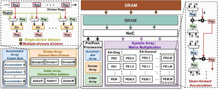
Figure 6: An illustration of our ViTALiTy accelerator, which adopts four memory hierarchies (i.e., DRAM, SRAM, NoC, and Regs) to enhance data locality and multiple chunks/sub-processors consisting of a few pre/post-processors and a systolic array to accelerate dedicated operations. Specifically, the pre-processors include an accumulator array for performing column(token)-wise summation, and a divider array and a adder array for conducting element-wise divisions and additions, respectively; In addition, the systolic array (SA) is partitioned into a smaller sub-array named SA-Diag to compute the matrix and diagonal matrix multiplications (i.e., $\mathbf{Q}\hat{\mathbf{k}}_{sum}^{T}$) considering their smaller number of multiplications, and a larger sub-array dubbed SA-General to process the remaining matrix multiplications (i.e., ${\mathbf{G}}=\hat{\mathbf{K}}^{T}\mathbf{V}$ and ${\mathbf{Q}}{\mathbf{G}}$).

Opportunity $1$: Reduced Number of Multiplications and Low-Cost Pre/Post-Processing. As mentioned above, our proposed Taylor attention can largely reduce the number of expensive multiplications and further avoid the use of the hardware unfriendly softmax operation, while introducing a few low-cost pre/post-processing steps. As such, our Taylor attention in some sense trades higher-cost multiplications and softmax operation with lower-cost pre/post-processing steps. Specifically, as formulated in Eq. (1), our attention achieves $(\mathbf{n}/\mathbf{d})\times$ reduction in the number of multiplications, where the number of tokens $\mathbf{n}$ is in general much larger than that of the feature dimension $\mathbf{d}$ in ViTs, leading to $\mathbf{n}/\mathbf{d}>>1$ (e.g., $\mathbf{n}/\mathbf{d}\approx 3$ in DeiT models [38], and $12.25$, $3$, $1$ for the three stages in LeViT-128/128s [20], respectively); WHile different from the three-step operations in the vanilla attention (see the bottom of Table II), our Taylor attention introduces several light-weight pre/post-processing steps to cooperate with the reduced number of matrix multiplications, i.e., as shown in Algorithm 1, the Steps 1 and 3 for pre-processing the keys and values via column-wise accumulations and element-wise additions, respectively, the post-processing in Steps 4 and 5 via element-wise additions, and the post-processing in Step 6 via row-wise divisions. Note that although row-wise divisions are also used in the softmax operation of the vanilla attention, our Taylor attention reduces the number of divisions by $(\mathbf{n}/\mathbf{d})\times$ (see Eq. (3)) as discussed above. Therefore, there exists an opportunity for the dedicated accelerator design to fully unleash the hardware efficiency benefits of our proposed Taylor attention’s property of “trades higher-cost multiplications and softmax operation with lower-cost pre/post-processing steps”.

Opportunity $2$: Data Dependency across Different Steps. As summarized in Algorithm 1, there exists data dependency in the sequentially processed steps of our Taylor attention. For example, 1) the generated mean-centering key $\mathbf{\hat{K}}$ in Step $1$ serves as the input for computing both the global context matrix $\mathbf{G}$ in Step $2$ and the column sum of keys $\mathbf{\hat{k}_{sum}}$ in Step $3$; 2) Both the obtained Taylor denominator $\mathbf{t_{D}}$ in Step $4$ and the Taylor numerator $\mathbf{T_{N}}$ in Step $5$ are then used to compute the final Taylor attention score $\mathbf{Z}$ in Step $6$. Such data dependency can cause large latency when accelerating the corresponding ViTs if not properly handled. For example, the computationally light pre/post-processing steps in our Taylor attention can account for about 50% of the total ViT’s profiling latency on the edge GPU, as shown in Table II. Hence, it is important for a dedicated accelerator to be equipped with proper pipeline designs to avoid the latency bottleneck due to the sequential execution pattern.

IV-B ViTALiTy Accelerator: Micro-Architecture

Motivation. As discussed in Opportunity $1$, in addition to matrix multiplications, our ViTALiTy accelerator is also expected to support column-wise accumulations, element-wise additions, and row-wise divisions for pre/post-processing steps of the ViTALiTy algorithm. To achieve this goal, two typical designs can be considered: 1) a single processor with reconfigurable processing units to simultaneously support all the aforementioned four types of operations, where the key is to minimize the overhead of supporting the required reconfigurability; and 2) a chunk-based accelerator design integrating multiple chunks/sub-accelerators with each dedicating to each type of operation, of which the advantage is that the reconfigurability overhead can be avoided but each chunk has a smaller amount of resources given the overall area constraint. Considering that the pre/post-processing steps in our ViTALiTy algorithm contain mostly low-cost hardware efficient operations, we adopt the latter design with a larger chunk for computing the expensive multiplications and smaller chunks for handling other low-cost steps.

Overview. As shown in Fig. 6, our ViTALiTy accelerator adopts 1) a four-level memory hierarchy including DRAM, SRAM, Network on Chip (NoC), and registers (Regs) within each computation unit to facilitate data reuses, and 2) a multi-chunk design that integrates multiple dedicated chunks/sub-processors, including a few pre/post-processors and a systolic array for supporting the diverse operators in our Taylor attention. In particular, the pre/post-processors consist of an accumulator array, a divider array, and an adder array for performing column(token)-wise summation, element-wise divisions, and element-wise additions, respectively. Specifically, the accumulator array is to pre-process the keys and values for generating corresponding column summations via accumulating all elements along the column/token dimension, i.e., computing the column summation of the keys $\mathbf{1}_{n}^{T}\mathbf{K}$ (see Step $1$ in Algorithm 1) and the column summation of both the mean-centering keys $\hat{\mathbf{k}}_{sum}$ and values ${\mathbf{v}}_{sum}$ (see Step $3$); The divider array is to process element-wise divisions in our Taylor attention, i.e., dividing the elements in the column summation matrix $\mathbf{1}_{n}^{T}\mathbf{K}$ by the column/token dimension $n$ to obtain the column/token-wise mean matrix $\hat{\mathbf{K}}$ (single-divisor division, see Step $1$ in Algorithm 1) as well as conducting the division between the Taylor numerator matrix $T_{N}$ and the diagonal Taylor denominator matrix $t_{D}$ to generate the final Taylor attention score $\mathbf{Z}$ (multiple-divisors division, see Step $6$). As such, as illustrated in Fig. 6 (see the upper left part), the divider array is designed to be reconfigurable for supporting both ❶ single-divisor division and ❷ multiple-divisors division patterns; In addition, the adder array is to perform the elements-wise additions/subtractions for obtaining the mean-centering keys $\hat{\mathbf{K}}$ in Step $1$, the Taylor denominator $\mathbf{t}_{D}$ in Step $4$, and the Taylor numerator $\mathbf{T}_{N}$ in Step $5$.

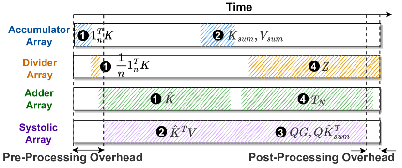
Figure 7: Illustrating the intra-layer pipeline design that minimizes both the pre- and post-processing overheads for enhancing the overall throughput.

Another important block in our ViTALiTy accelerator is the systolic array which is to process matrix multiplications in our Taylor attention, i.e., $\mathbf{G}=\hat{\mathbf{K}}^{T}\mathbf{V}$ in Step $2$, $\mathbf{Q}\hat{\mathbf{k}}_{sum}^{T}$ in Step $4$, and ${\mathbf{Q}}{\mathbf{G}}$ in Step $5$. Specifically, the systolic array is partitioned into two parts donated as SA-Diag and SA-General, respectively, to compute $\mathbf{Q}\hat{\mathbf{k}}_{sum}^{T}$ and ${\mathbf{Q}}{\mathbf{G}}$ in parallel for 1) simultaneously calculating the Taylor denominator and numerator and thus can be then pipelined with the computation of the Taylor attention score in Step 6 to improve the overall throughput (see Section IV-C for details) and 2) reducing the data access cost of the queries $Q$ to improve the energy efficiency (see Section IV-D for details). As the number of multiplications in $\mathbf{Q}\hat{\mathbf{k}}_{sum}^{T}$ is much smaller than that in ${\mathbf{Q}}{\mathbf{G}}$, i.e., the former is $n\times d\times 1$ while the latter is $n\times d\times d$, it is natural to allocate fewer PEs (Processing Elements), i.e., only one PE column, for the SA-Diag sub-array. In addition to process matrix multiplications, the systolic array is also reused to compute the preceding linear projection and subsequent MLP module, considering their operations are similar.

IV-C ViTALiTy Accelerator: Intra-Layer Pipeline Design

As listed in Table II, general computing platforms, e.g., GPUs, cannot leverage the theoretical benefits of ViTALiTy’s Taylor attention for achieving actual hardware efficiency. One of the reasons is that the sequentially executed computation steps in our Taylor attention require dedicated pipeline design. Considering the data dependency across different steps (see Opportunity $2$) and our multi-chunk micro-architecture (see Section IV-B), our ViTALiTy accelerator adopts an intra-layer pipeline design to enhance the overall throughput, as illustrated in Fig. 7 and discussed below:

1. The accumulator and divider arrays first pre-process ${\mathbf{K}}$ to generate the column-wise mean of the keys $\overline{\mathbf{K}}$, where each element is then subtracted by the elements in the corresponding column of K via the adder array to obtain the mean-centering keys $\hat{\mathbf{K}}$ (see Step $1$ of Algorithm 1).

2. While computing $\hat{\mathbf{K}}$ via the adder array, the already generated ones are sent to both the systolic array to multiply with ${\mathbf{V}}$ for computing the global context matrix ${\mathbf{G}}$ (i.e., Step $2$ of Algorithm 1; see Fig. 9(b) and Section IV-D for details) to reduce the pre-processing overhead, and the accumulator array along with ${\mathbf{V}}$ to generate $\hat{\mathbf{k}}_{sum}$ and ${\mathbf{v}}_{sum}$ (see Step $3$) for decreasing accumulator array’s idle time.

3. Once obtaining both $\mathbf{G}$ and ${\mathbf{k}}_{sum}^{T}$, the systolic array is reused and then partitioned into SA-General and SA-Diag to simultaneously process ${\mathbf{Q}\mathbf{G}}$ and $\mathbf{Q}\hat{\mathbf{k}}_{sum}^{T}$ with ${\mathbf{Q}}$ being broadcasted to both sub-arrays (see Fig. 9(c) and Section IV-D for details).

4. After calculating the first element in $\mathbf{Q}\hat{\mathbf{k}}_{sum}^{T}$ and the first row of ${\mathbf{Q}}{\mathbf{G}}$, an extra adder unit and the adder array are used to compute the Taylor denominator $t_{D}$ and numerator $\mathbf{T}_{N}$ in Steps $4$ and $5$, respectively, which are then processed by the divider arrray to generate the final Taylor attention score $\mathbf{Z}$ in Step $6$ of Algorithm 1. This helps fuse the post-processing steps with matrix multiplications for reducing the post-processing overhead.

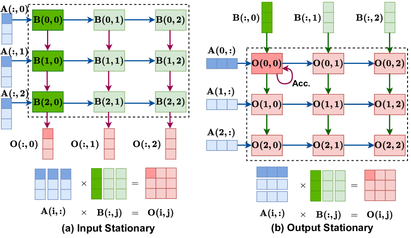
Figure 8: Illustrating two typical dataflows for dense matrix multiplications: (a) input stationary and (b) output stationary, where the partial sums are down-forward accumulated in the former and inner-PE accumulated in the latter.

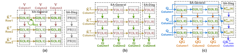
Figure 9: Illustrating two potential dataflows for ViTALiTy accelerator’s systolic array: 1) G-stationary adopts (a) output stationary to compute $\mathbf{G}=\hat{\mathbf{K}}^{T}\mathbf{V}$ and (c) input stationary to process both $\mathbf{Q}\mathbf{G}$ and $\mathbf{Q}\hat{\mathbf{K}}^{T}_{sum}$ for keeping $\mathbf{G}$ stationary within the PEs, and 2) down-forward accumulation dataflow that adopts input stationary to handle all the multiplications (see (b) and (c)).

IV-D ViTALiTy Acc.: Down-Forward Accumulation Dataflow

As matrix multiplication is the cost-dominant operation in our proposed Taylor attention, the adopted dataflow that determines how to temporally and spatially map multiplications onto the PE array is crucial to the achievable hardware efficiency of ViTALiTy accelerator. For better understanding, we first introduce two typical dataflows for processing dense matrix multiplications: input and output stationary. As illustrated in Fig. 8, assuming $\mathbf{O}=\mathbf{A}\mathbf{B}$, we can see that 1) for input stationary, $\mathbf{B}$ stays stationary in the PE array and each column of $\mathbf{A}$ is horizontally traversed to one PE row, where each PE column is responsible for processing one vector dot-product between one row of $\mathbf{A}$ and one column of $\mathbf{B}$ and the partial sums are then down-forward accumulated to gather the final outputs at the bottom-most PEs (down-forward accumulation); 2) For output stationary, each row of $\mathbf{A}$ instead is horizontally sent to one PE row while each column of $\mathbf{B}$ is vertically mapped to one PE column, where each PE computes the vector dot-product between one row of $\mathbf{A}$ and one column of $\mathbf{B}$ and the partial sums are then temporally accumulated within the PEs (inner-PE accumulation).

As discussed in Section IV-C, our systolic array is leveraged to first perform $\mathbf{G}=\hat{\mathbf{K}}^{T}\mathbf{V}$ and then reused and partitioned into two sub-blocks dubbed SA-General and SA-Diag to simultaneously compute $\mathbf{Q}\mathbf{G}$ and $\mathbf{Q}\hat{\mathbf{k}}^{T}_{sum}$, respectively. Considering the two typical dataflows above for one single dense matrix multiplication, there exist two potential dataflows for handling the consecutive matrix multiplications in our Taylor attention (i.e., $\mathbf{G}=\hat{\mathbf{K}}^{T}\mathbf{V}$, $\mathbf{Q}\mathbf{G}$, and $\mathbf{Q}\hat{\mathbf{k}}^{T}_{sum}$ in Algorithm 1): G-stationary and down-forward accumulation dataflows.

Specifically, 1) as $\mathbf{G}$ serves as both the output of $\mathbf{G}=\hat{\mathbf{K}}^{T}\mathbf{V}$ and the input of $\mathbf{Q}\mathbf{G}$, G-stationary is the most intuitive dataflow that adopts output-stationary for computing $\mathbf{G}=\hat{\mathbf{K}}^{T}\mathbf{V}$ and then keeps $\mathbf{G}$ stationary within the PEs to serve as the input for computing $\mathbf{Q}\mathbf{G}$ via input-stationary. As such, the PEs need to be reconfigurable for simultaneously supporting both inner-PE accumulation for output stationary (see Fig. 9 (a)) and down-forward accumulation for input stationary (see Fig. 9 (c)); 2) Another alternative is the down-forward accumulation dataflow that adopts input-stationary for computing all the matrix multiplications in our attention, i.e., $\mathbf{V}$ stays stationary when computing $\hat{\mathbf{K}}^{T}\mathbf{V}$ (see Fig. 9 (b)) while $\mathbf{G}$ and $\hat{\mathbf{k}}^{T}_{sum}$ remain stationary in the SA-General and SA-Diag sub-blocks, respectively, with $\mathbf{Q}$ being broadcasted to process $\mathbf{Q}\mathbf{G}$ and $\mathbf{Q}\hat{\mathbf{k}}^{T}_{sum}$ in parallel (see Fig. 9 (c)). Hence, the former enhances data locality of $\mathbf{G}$ for minimizing its data access cost but requires overhead to reconfigure the PEs for simultaneously supporting the above two accumulation patterns, while the latter simplifies the PE design at a cost of increased data access cost. As the energy consumed by the systolic array dominates the overall energy cost instead of the data access cost from SRAM (see Table V), we adopts the down-forward accumulation dataflow for boosting the overall energy efficiency (see ablation study in Section V-D).

V Evaluation and Analysis

V-A Experiment Setting

Models and Methods. We evaluate on popular ViT models, including 1) vanilla ViTs - DeiT-Base/Small/Tiny [38], 2) lightweight ViT models - MobileViT-xxs/xs [30], and 3) hybrid ViT models - LeViT-128s/128 [20]. Various methods are benchmarked with: Baseline (ViTs with vanilla softmax attentions), Sparse (Sanger [28] with a sparsity threshold of $T=0.02$), LowRank (ViTs with Taylor attentions on pre-trained models), and ViTALiTy (trained using both low-rank and sparse attentions, but inference with only low-rank attentions). While Sanger is originally designed for NLP tasks, we implement its algorithm to train the ViT models. Model accuracy is reported on the ImageNet[14] validation dataset.

Hardware Settings. To verify the effectiveness of our ViTALiTy accelerator, we consider three general computing hardware platforms, including 1) CPU (Intel(R) Xeon(R) Gold 6230), 2) Edge GPU (NVIDIA Tegra X2), and 3) GPU (NVIDIA 2080Ti), and 4) a SOTA dedicated attention accelerator Sanger [28]. Note that for fair comparisons, we scale up ViTALiTy’s hardware resource to be comparable with the aforementioned baselines. Specifically, when benchmarking with the general computing platforms, we follow [33] to scale up ViTALiTy’s accelerator to have a comparable peak throughput as that of the platform, and for benchmarking with Sparse (Sanger), we adopt the comparable hardware budgets as Sanger. We compare our dedicated accelerator over these four baselines in terms of both energy efficiency and speedup.

V-B Implementation

TABLE III: Configurations of ViTALiTy and Sanger [28] accelerators.

ViTALiTy	Component	Parameter	Area ($mm^{2}$)	Power (mW)
Pre/Post- Processors	Accumulator Array	$64\times 1$ $16$-bit	$0.209$	$92.83$
	Adder Array	$64\times 1$ $16$-bit	$0.012$	$6.34$
	Divider Array	$64\times 1$ $16$-bit	$0.562$	$46.26$
Systolic Array	SA-General	$64\times 64$ $16$-bit	$3.595$	$1277$
	SA-Diag	$64\times 1$ $16$-bit	$0.053$	$15.18$
Memory	[$\mathbf{Q}$, $\mathbf{K}$, $\mathbf{V}$, $\mathbf{O}$]	$50$ KB$\times 4$	$0.792$	$22.9$
Overall		$28$ nm	$\mathbf{5.223}$	$\mathbf{1460}$
Sanger	Component	Parameter	Area ($mm^{2}$)	Power (mW)
Pre/Post- Processors	Pre-Processor	64 $\times$ $64$ $44$-bit	$0.430$	$182.8$
	Pack & Split	$64\times 64$ $1$-bit	$0.016$	$0.64$
	Divider Array	$64\times 1$ $16$-bit	$0.562$	$46.26$
Systolic Array	RePE	$64\times 16$ $16$-bit	$3.393$	$1198.35$
	EXP	$64\times 1$ $16$-bit
Memory	[$\mathbf{Q}$, $\mathbf{K}$, $\mathbf{V}$, $\mathbf{O}$]	$50$ KB $\times 4$	$0.792$	22.90
Overall		$28$ nm	$\mathbf{5.194}$	$\mathbf{1450}$

Software Implementation. We fine-tune the pre-trained ViT models from [43], and follow the training recipe in [38]. For inference, we implement Algorithm 1 for DeiT, MobileViT and LeViT models. To further boost accuracy, we apply token based knowledge distillation [38] during training.

Hardware Implementation. To evaluate the performance of ViTALiTy, we implement a cycle-accurate simulator for our dedicated accelerator to obtain fast and reliable estimations, which are verified against the RTL implementation to ensure the correctness. The adopted unit energy and area are synthesized on a $28$ nm CMOS technology using Synopsys tools (e.g., Design Compiler for gate-level netlist [1]) at a frequency of $500$ MHz. For a fair comparison, we also implement a cycle-accurate simulator for the baseline accelerator, Sanger [28], and compare the simulated results with the reported performance in the Sanger [28] paper to ensure the correctness. As shown in Table III, we evaluate both ViTALiTy accelerator and Sanger accelerator under a comparable area and power when being synthesized under the same CMOS technology and clock frequency.

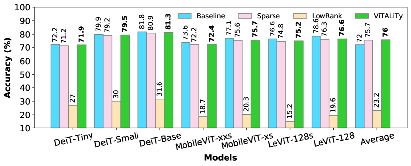
Figure 10: Accuracy comparison between ViTALiTy and other methods across various ViT models. Here, Baseline is vanilla softmax attention, Sparse is Sanger [28], and LowRank refers to applying linear Taylor attention on pre-trained model. ViTALiTy outperforms both Sparse and LowRank.

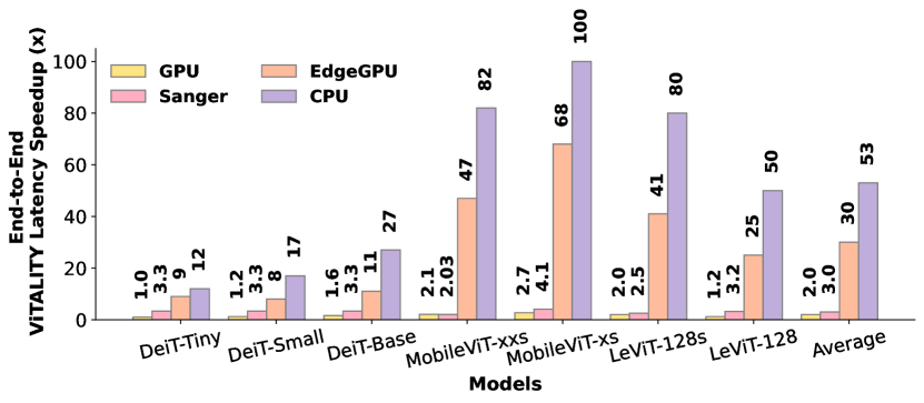
Figure 11: End-to-End Latency Speedup of ViTALiTY accelerator.

TABLE IV: Accuracy vs FLOPS (Attention) tradeoff for various methods.

Method	Type	Accuracy (%)	FLOPs (G)
Baseline	Quadratic	$72.2$	$0.50$
ViTALiTy (ours)	Linear	71.9	0.33
Linformer [41]	Linear	$69.5$	$0.35$
Performer [11]	Linear	$68.3$	$0.40$
Sanger [28]	Sparse	$71.2$	$0.33$
SViTE [9]	Sparse	$71.7$	$0.38$
UVC [47]	Sparse	$71.8$	$0.30$

V-C Performance Analysis

Here, we analyze the performance of the proposed ViTALiTy in terms of accuracy, latency, and energy efficiency.

Accuracy. In Fig. 10, we demonstrate the accuracy achieved by various methods. We observe that training the various ViT models with ViTALiTy consistently improves the model accuracy with $\textbf{45\%}-\textbf{60\%}$ on the LowRank method, and with $\textbf{0.1\%}-\textbf{0.7\%}$ on the Sparse method. This demonstrates that the proposed ViTALiTy is a version of Scatterbrain [6] where the combination of low-rank and sparse approximation training achieves better accuracy than the individual components. Once the model is trained, in contrast to Scatterbrain [6] and Sparse, ViTALiTy simply employs the low-rank component for inference by computing the linear Taylor Attention to achieve this improved accuracy without the runtime overhead of sparse attention. It is worth recalling that ViTALiTy uses sparse approximation for capturing strong connections during training compared to vanilla softmax attention in Baseline. Hence, the accuracy of ViTALiTy falls short of Baseline accuracy by $0.3\%-2\%$ as expected. We trade the above accuracy drop of ViTALiTy trained models with the latency speedup and energy efficiency achieved using linear attention and dedicated accelerator for inference compared to running Baseline method with full softmax attention incurring quadratic costs. Table IV shows that ViTALiTy outperforms other linear and sparse attention with better or comparable (UVC) accuracy versus FLOPs (attention) tradeoff.

Latency Speedup. Fig. 11 shows latency speedup of our ViTALiTy accelerator where it consistently outperforms all the aforementioned hardware baselines, validating the effectiveness of our proposed linear Taylor Attention algorithm on reducing the computation complexity of attention, and proposed intra-layer pipeline design of the accelerator in boosting the overall throughput. Specifically, on benchmarking the acceleration of core attention on general platforms, our ViTALiTy accelerator achieves an average $\textbf{236}\times$, $\textbf{239}\times$, and $\textbf{9}\times$ speedup over CPU, Edge GPU, and GPU, respectively. When comparing the end-to-end latency, our ViTALiTy accelerator is $\textbf{53}\times$, $\textbf{30}\times$, and $\textbf{2}\times$ faster over CPU, Edge GPU, and GPU, respectively. Furthermore, compared to Sanger [28], ViTALiTy gains an average $\textbf{7}\times$ speedup on the attention acceleration with $\textbf{3}\times$ speedup on end-to-end acceleration. Additionally, we verify the effectiveness of ViTALiTy accelerator by comparing it with the accelerator SALO [35] which is designed for LongFormer [3] linear attention. It enables hybrid sparse attention mechanisms including sliding window attention, dilated window attention, and global attention. When comparing both accelerators under the same hardware budget for DeiT-Tiny and DeiT-Small models, ViTALiTy achieves up to 4.7$\times$ and 5.0$\times$ speedup on the attention acceleration, respectively, under a comparable accuracy.

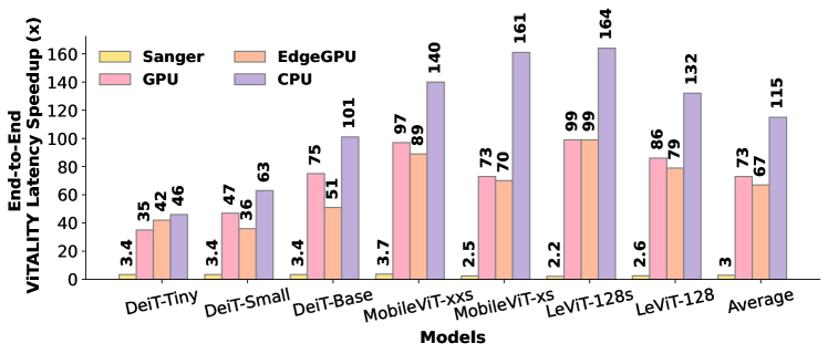
Figure 12: Energy Efficiency comparison of ViTALiTY accelerator.

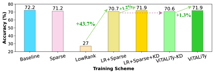
Figure 13: Ablation study of ViTALiTy on DeiT-Tiny model. LR denotes LowRank, and KD denotes Knowledge Distillation.

Energy Efficiency. Fig.12 shows the ViTALiTy accelerator’s improvement in energy efficiency over other hardware baselines, demonstrating the advantage of its co-design framework. For core attention steps, our ViTALiTy accelerator achieves an average $\textbf{537}\times$, $\textbf{309}\times$, $\textbf{187}\times$, and $\textbf{6}\times$ better energy efficiency , and for the end-to-end performance, it offers an average $\textbf{115}\times$, $\textbf{67}\times$, $\textbf{73}\times$, and $\textbf{3}\times$ better energy efficiency, over CPU, Edge GPU, GPU, and Sanger [28], respectively.

V-D Ablation Study

Here, we discuss the ablation study of ViTALiTy training scheme on the DeiT-Tiny model, the effect of sparsity threshold on the model accuracy, and dataflow in accelerator design.

Training Scheme. Fig. 13 demonstrates the accuracy obtained by various training schemes as part of our ablation study on the proposed ViTaLiTy method. We recall that the ViTaLiTy method involves training ViT by unifying linear Taylor Attention as LowRank component, and the Sanger [28] induced sparsity mask with threshold, $T=0.5$ as the Sparse component. We also incorporate token-based knowledge distillation (KD). For inference, ViTaLiTy simply uses the linear Taylor Attention without any additional sparse component. Compared to Baseline accuracy 72.2% with softmax attention, we observe that Sparse (Sanger [28], $T=0.02$) achieves 71.2% accuracy.

☞ Sparse boosts the accuracy of LowRank

LowRank method uses linear Taylor Attention as drop-in replacement of softmax attention in pre-trained ViT models for inference and suffers from poor model accuracy of 27%. This supports our claim in Section III-B that it is unlikely all (query,key) pairs have similarity within [-1,1). On unifying the above linear Taylor Attention (low-rank) and Sanger [28] sparsity with $T=0.5$ as LowRank+Sparse for fine-tuning the model and in inference, we observe improved accuracy of 70.7% (with boost of $43.7\%$ over LowRank method). This demonstrates that the model now successfully captures the strong connections using the Sparse component which was missing using just the linear Taylor Attention from the LowRank method. Applying KD during fine-tuning of model additionally improves the accuracy by $1.2\%$ to 71.9%.

☞ Sparse is not required during inference

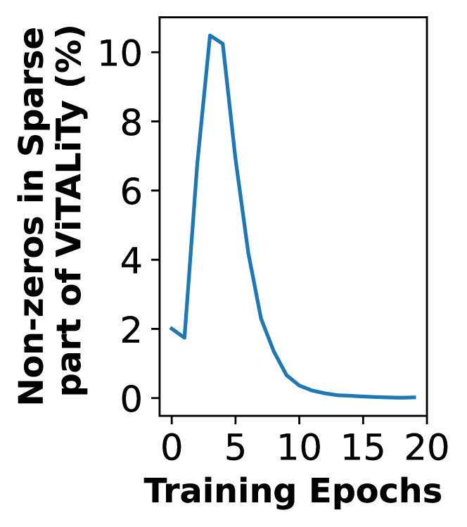
Figure 14: Sparse component vanishes after $10$ epochs, hence, can be dropped during inference.

Fig. 14 shows that the sparse component in ViTALiTy-KD vanishes after boosting the accuracy in initial training epochs of DeiT-Tiny. Hence, it can be dropped during inference with negligible effect on model accuracy after fine-tuning the model with unified LowRank+Sparse. This critical observation implies that the Sparse acts as a regularizer for generalizing the linear Taylor Attention such that during inference, the corresponding dense LowRank component is self-sufficient. This empowers the proposed ViTALiTy method to deploy ViT models on edge devices by avoiding the overhead of runtime sparsity computation during inference for various inputs. Applying KD further boosts the accuracy of ViTALiTy by $1.3\%$ to 71.9% which matches the LowRank+Sparse+KD accuracy attained by additionally computing the sparse component during inference.

Sparsity Threshold. Fig. 15 illustrates the effect of sparsity thresholds [$0.002,0.02,0.2,0.5,0.9$] on DeiT-Tiny model accuracy. The Sparse method achieves accuracy of $71.2\%$ (Fig. 13) using the default threshold, $T=0.02$ defined in Sanger [29]. By incorporating LowRank+Sparse+KD, the model achieves slightly improved accuracy of $71.3\%$ at same threshold value, whereas, by using ViTALiTy which drops the sparse component during inference, the model retains the same accuracy of $71.2\%$ as the Sparse method.

☞ LowRank renders Sparse to exhibit high sparsity

As the sparsity threshold increases, more zeros are introduced in the sparse attention matrix generated by applying Sanger sparsity masks on quantized softmax attention. This reduces the contribution of sparse component relative to the low-rank component (linear Taylor Attention) in LowRank+Sparse+KD, and ViTALiTy methods. When $T=1$, the sparse component vanishes completely during training and inference which leaves only the low-rank component, thereby, signalling accuracy drop when $T=0.9$ as demonstrated in Fig. 15.

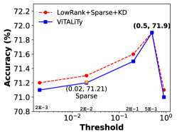
Figure 15: Effect of sparsity threshold on DeiT-Tiny model accuracy. Optimal $T=0.5$.

For low threshold values, there is low sparsity which implies large contribution of softmax attention which overpowers the low-rank properties of linear Taylor Attention. As sparsity threshold increases, LowRank component becomes more prominent as the approximation of softmax attention leads to highly sparse matrix. This helps improve the model accuracy for both methods (Fig. 15). We observe the optimal threshold value is empirically achieved at $T=0.5$, where, the low-rank properties of linear Taylor Attention in ViTALiTy renders the sparse attention matrix to exhibit high sparsity during training which yields the best accuracy of $71.9\%$. At this threshold, ViTALiTy with no sparse component during inference matches the accuracy of LowRank+Sparse+KD.

Dataflow in Systolic Array.

TABLE V: Energy comparison of G-stationary and proposed down-forward accumulation dataflows for Taylor Attention

Energy ($10^{-6}J$)	DeiT-Base		MobileViT-xxs		MobileViT-xs		LeViT-128s		LeViT-128
	GS	Ours	GS	Ours	GS	Ours	GS	Ours	GS	Ours
Data Access	2.92	$3.76$	0.12	$0.15$	0.23	$0.28$	0.09	$0.12$	0.14	$0.19$
Other Processors	$3.92$	$3.92$	$0.15$	$0.15$	$0.23$	$0.23$	$0.12$	$0.12$	$0.19$	$0.19$
Systolic Array	$215$	191	$13.2$	10.3	$23.3$	20.1	$11.1$	9.03	$16.6$	13.3
Overall	$222$	198	$13.5$	10.6	$23.8$	20.6	$11.3$	9.27	$16.9$	13.7

In Table V, we observe that the (1) overall energy consumption of our proposed down-forward accumulation dataflow is consistently lower than the G-Stationary (GS) dataflow when benchmarking Taylor Attention on various ViT models, validating the effectiveness of the former for boosting energy efficiency, (2) G-Stationary dataflow has lower data access cost by keeping the generated $\mathbf{G}=\hat{\mathbf{K}}^{T}\mathbf{V}$ stationary inner PEs which sequentially compute $\mathbf{Q}\mathbf{G}$ for enhancing data locality, and (3) Proposed down-forward accumulation dataflow instead reduces the more dominant systolic array cost by simplifying the PE design by advocating for input stationary when computing the matrix multiplications in the linear Taylor Attention.

TABLE VI: Attention types and corresponding Pre/Post-Processors for typical linear attention Transformers.

Attention Types	Models	Details	Pre/Post-Processors
Low-Rank	Linformer[41]	Reduce token dim. of $\mathbf{K}$/$\mathbf{V}$	Exp. Div.
Kernel-Based	Efficient Attention [36]	$\phi()$= softmax()	Exp. Div.
	Performer [11]	PORF	Exp. Div. Add.
	Linear Transformer [24]	$\phi()$=elu() + 1	Exp. Div. Add.
Taylor-Based	ViTALiTy (Ours)	See Algorithm 1	Acc. Div. Add.

Extension of ViTALiTy Accelerator. We summarize typical linear attention Transformers in Table VI, where attention mechanisms are categorized into the low-rank based one [41], kernel-based ones [36, 11, 24], and our proposed Taylor Attention. We observe that our accelerator can be easily extended to accelerate diverse efficient Transformers with dedicated pre/post-processors for corresponding similarity ($\phi$) functions (e.g., softmax for [41] and [36], PORF for [11]), and generic systolic array for matrix multiplications.

VI Conclusions

We present a new algorithm and hardware co-designed ViT framework dubbed ViTALiTy that unifies the low-rank linear Taylor attention with a sparse approximated attention during training for boosting the achievable accuracy and then drops the sparse component during inference for improving the acceleration efficiency without hurting the accuracy. Orthogonal to existing sparsity-based accelerators dedicated to NLP, our ViTALiTy accelerator is developed to better exploit the resulting algorithmic properties of ViTALiTy’s linear attention for boosting hardware efficiency during inference. ViTALiTy achieves up to $\textbf{3}\times$ end-to-end latency speedup with $\textbf{3}\times$ energy efficiency over Sanger [28] under a comparable accuracy.

References

- [1] “Synopsys design compiler.” [Online]. Available: https://www.synopsys.com/implementation-and-signoff/rtl-synthesis-test/dc-ultra.html
- [2] I. Beltagy, M. E. Peters, and A. Cohan, “Longformer: The long-document transformer,” arXiv preprint arXiv:2004.05150, 2020.
- [3] I. Beltagy, M. E. Peters, and A. Cohan, “Longformer: The long-document transformer,” ArXiv, vol. abs/2004.05150, 2020.
- [4] H. Cai, C. Gan, and S. Han, “Efficientvit: Enhanced linear attention for high-resolution low-computation visual recognition,” 2022. [Online]. Available: https://arxiv.org/abs/2205.14756
- [5] N. Carion, F. Massa, G. Synnaeve, N. Usunier, A. Kirillov, and S. Zagoruyko, “End-to-end object detection with transformers,” in European conference on computer vision. Springer, 2020, pp. 213–229.
- [6] B. Chen, T. Dao, E. Winsor, Z. Song, A. Rudra, and C. Ré, “Scatterbrain: Unifying sparse and low-rank attention,” in Advances in Neural Information Processing Systems, A. Beygelzimer, Y. Dauphin, P. Liang, and J. W. Vaughan, Eds., 2021. [Online]. Available: https://openreview.net/forum?id=SehIKudiIo1
- [7] C.-F. R. Chen, Q. Fan, and R. Panda, “Crossvit: Cross-attention multi-scale vision transformer for image classification,” in Proceedings of the IEEE/CVF International Conference on Computer Vision, 2021, pp. 357–366.
- [8] H. Chen, Z. Luo, J. Zhang, L. Zhou, X. Bai, Z. Hu, C.-L. Tai, and L. Quan, “Learning to match features with seeded graph matching network,” in Proceedings of the IEEE/CVF International Conference on Computer Vision (ICCV), October 2021, pp. 6301–6310.
- [9] T. Chen, Y. Cheng, Z. Gan, L. Yuan, L. Zhang, and Z. Wang, “Chasing sparsity in vision transformers: An end-to-end exploration,” Advances in Neural Information Processing Systems, vol. 34, pp. 19 974–19 988, 2021.
- [10] R. Child, S. Gray, A. Radford, and I. Sutskever, “Generating long sequences with sparse transformers,” arXiv preprint arXiv:1904.10509, 2019.
- [11] K. M. Choromanski, V. Likhosherstov, D. Dohan, X. Song, A. Gane, T. Sarlos, P. Hawkins, J. Q. Davis, A. Mohiuddin, L. Kaiser, D. B. Belanger, L. J. Colwell, and A. Weller, “Rethinking attention with performers,” in International Conference on Learning Representations, 2021. [Online]. Available: https://openreview.net/forum?id=Ua6zuk0WRH
- [12] G. M. Correia, V. Niculae, and A. F. Martins, “Adaptively sparse transformers,” arXiv preprint arXiv:1909.00015, 2019.
- [13] B. Cui, Y. Li, M. Chen, and Z. Zhang, “Fine-tune bert with sparse self-attention mechanism,” in Proceedings of the 2019 conference on empirical methods in natural language processing and the 9th international joint conference on natural language processing (EMNLP-IJCNLP), 2019, pp. 3548–3553.
- [14] J. Deng, W. Dong, R. Socher, L.-J. Li, K. Li, and L. Fei-Fei, “Imagenet: A large-scale hierarchical image database,” in 2009 IEEE conference on computer vision and pattern recognition. Ieee, 2009, pp. 248–255.
- [15] J. Devlin, M.-W. Chang, K. Lee, and K. Toutanova, “Bert: Pre-training of deep bidirectional transformers for language understanding,” arXiv preprint arXiv:1810.04805, 2018.
- [16] A. Dosovitskiy, L. Beyer, A. Kolesnikov, D. Weissenborn, X. Zhai, T. Unterthiner, M. Dehghani, M. Minderer, G. Heigold, S. Gelly, J. Uszkoreit, and N. Houlsby, “An image is worth 16x16 words: Transformers for image recognition at scale,” in International Conference on Learning Representations, 2021.
- [17] H. Germain, V. Lepetit, and G. Bourmaud, “Visual correspondence hallucination,” in International Conference on Learning Representations, 2022. [Online]. Available: https://openreview.net/forum?id=jaLDP8Hp_gc
- [18] C. Gong, D. Wang, M. Li, X. Chen, Z. Yan, Y. Tian, qiang liu, and V. Chandra, “NASVit: Neural architecture search for efficient vision transformers with gradient conflict aware supernet training,” in International Conference on Learning Representations, 2022.
- [19] Google LLC., “Pixel 3,” https://g.co/kgs/pVRc1Y, accessed 2020-09-01.
- [20] B. Graham, A. El-Nouby, H. Touvron, P. Stock, A. Joulin, H. Jegou, and M. Douze, “Levit: A vision transformer in convnet’s clothing for faster inference,” in Proceedings of the IEEE/CVF International Conference on Computer Vision (ICCV), October 2021, pp. 12 259–12 269.
- [21] T. J. Ham, S. J. Jung, S. Kim, Y. H. Oh, Y. Park, Y. Song, J.-H. Park, S. Lee, K. Park, J. W. Lee et al., “A^ 3: Accelerating attention mechanisms in neural networks with approximation,” in 2020 IEEE International Symposium on High Performance Computer Architecture (HPCA). IEEE, 2020, pp. 328–341.
- [22] T. J. Ham, Y. Lee, S. H. Seo, S. Kim, H. Choi, S. J. Jung, and J. W. Lee, “Elsa: Hardware-software co-design for efficient, lightweight self-attention mechanism in neural networks,” in 2021 ACM/IEEE 48th Annual International Symposium on Computer Architecture (ISCA). IEEE, 2021, pp. 692–705.
- [23] B. Heo, S. Yun, D. Han, S. Chun, J. Choe, and S. J. Oh, “Rethinking spatial dimensions of vision transformers,” in Proceedings of the IEEE/CVF International Conference on Computer Vision, 2021, pp. 11 936–11 945.
- [24] A. Katharopoulos, A. Vyas, N. Pappas, and F. Fleuret, “Transformers are rnns: Fast autoregressive transformers with linear attention,” in International Conference on Machine Learning. PMLR, 2020, pp. 5156–5165.
- [25] N. Kitaev, L. Kaiser, and A. Levskaya, “Reformer: The efficient transformer,” in International Conference on Learning Representations, 2020. [Online]. Available: https://openreview.net/forum?id=rkgNKkHtvB
- [26] Z. Liu, Y. Lin, Y. Cao, H. Hu, Y. Wei, Z. Zhang, S. Lin, and B. Guo, “Swin transformer: Hierarchical vision transformer using shifted windows,” in Proceedings of the IEEE/CVF International Conference on Computer Vision, 2021, pp. 10 012–10 022.
- [27] Z. Liu, Y. Wang, K. Han, W. Zhang, S. Ma, and W. Gao, “Post-training quantization for vision transformer,” in Advances in Neural Information Processing Systems, M. Ranzato, A. Beygelzimer, Y. Dauphin, P. Liang, and J. W. Vaughan, Eds., vol. 34. Curran Associates, Inc., 2021, pp. 28 092–28 103.
- [28] L. Lu, Y. Jin, H. Bi, Z. Luo, P. Li, T. Wang, and Y. Liang, “Sanger: A co-design framework for enabling sparse attention using reconfigurable architecture,” ser. MICRO ’21. New York, NY, USA: Association for Computing Machinery, 2021, p. 977–991.
- [29] L. Lu, Y. Jin, H. Bi, Z. Luo, P. Li, T. Wang, and Y. Liang, “Sanger: A co-design framework for enabling sparse attention using reconfigurable architecture,” in MICRO-54: 54th Annual IEEE/ACM International Symposium on Microarchitecture, 2021, pp. 977–991.
- [30] S. Mehta and M. Rastegari, “Mobilevit: light-weight, general-purpose, and mobile-friendly vision transformer,” arXiv preprint arXiv:2110.02178, 2021.
- [31] NVIDIA Inc., “NVIDIA Jetson TX2,” https://www.nvidia.com/en-us/autonomous-machines/embedded-systems/jetson-tx2/, accessed 2020-09-01.
- [32] NVIDIA LLC., “GeForce RTX 2080 TI Graphics Card — NVIDIA,” 2021, https://www.nvidia.com/en-me/geforce/graphics-cards/rtx-2080-ti/, accessed 2020-09-01.
- [33] Z. Qu, L. Liu, F. Tu, Z. Chen, Y. Ding, and Y. Xie, “Dota: detect and omit weak attentions for scalable transformer acceleration,” in Proceedings of the 27th ACM International Conference on Architectural Support for Programming Languages and Operating Systems, 2022, pp. 14–26.
- [34] A. Radford, K. Narasimhan, T. Salimans, and I. Sutskever, “Improving language understanding by generative pre-training,” 2018.
- [35] G. Shen, J. Zhao, Q. Chen, J. Leng, C. Li, and M. Guo, “Salo: an efficient spatial accelerator enabling hybrid sparse attention mechanisms for long sequences,” Proceedings of the 59th ACM/IEEE Design Automation Conference, 2022.
- [36] Z. Shen, M. Zhang, H. Zhao, S. Yi, and H. Li, “Efficient attention: Attention with linear complexities,” in Proceedings of the IEEE/CVF winter conference on applications of computer vision, 2021, pp. 3531–3539.
- [37] S. Tang, J. Zhang, S. Zhu, and P. Tan, “Quadtree attention for vision transformers,” in International Conference on Learning Representations, 2022. [Online]. Available: https://openreview.net/forum?id=fR-EnKWL_Zb
- [38] H. Touvron, M. Cord, M. Douze, F. Massa, A. Sablayrolles, and H. Jegou, “Training data-efficient image transformers & distillation through attention,” in International Conference on Machine Learning, vol. 139, July 2021, pp. 10 347–10 357.
- [39] A. Vaswani, N. Shazeer, N. Parmar, J. Uszkoreit, L. Jones, A. N. Gomez, Ł. Kaiser, and I. Polosukhin, “Attention is all you need,” Advances in neural information processing systems, vol. 30, 2017.
- [40] H. Wang, Z. Zhang, and S. Han, “Spatten: Efficient sparse attention architecture with cascade token and head pruning,” in 2021 IEEE International Symposium on High-Performance Computer Architecture (HPCA). IEEE, 2021, pp. 97–110.
- [41] S. Wang, B. Z. Li, M. Khabsa, H. Fang, and H. Ma, “Linformer: Self-attention with linear complexity,” 2020. [Online]. Available: https://arxiv.org/abs/2006.04768
- [42] W. Wang, E. Xie, X. Li, D.-P. Fan, K. Song, D. Liang, T. Lu, P. Luo, and L. Shao, “Pyramid vision transformer: A versatile backbone for dense prediction without convolutions,” in Proceedings of the IEEE/CVF International Conference on Computer Vision, 2021, pp. 568–578.
- [43] R. Wightman, “Pytorch image models,” https://github.com/rwightman/pytorch-image-models, 2019.
- [44] H. Wu, B. Xiao, N. Codella, M. Liu, X. Dai, L. Yuan, and L. Zhang, “Cvt: Introducing convolutions to vision transformers,” 2021.
- [45] J. Yang, C. Li, P. Zhang, X. Dai, B. Xiao, L. Yuan, and J. Gao, “Focal self-attention for local-global interactions in vision transformers,” arXiv preprint arXiv:2107.00641, 2021.
- [46] L. Ye, M. Rochan, Z. Liu, and Y. Wang, “Cross-modal self-attention network for referring image segmentation,” in Proceedings of the IEEE/CVF Conference on Computer Vision and Pattern Recognition, 2019, pp. 10 502–10 511.
- [47] S. Yu, T. Chen, J. Shen, H. Yuan, J. Tan, S. Yang, J. Liu, and Z. Wang, “Unified visual transformer compression,” arXiv preprint arXiv:2203.08243, 2022.
- [48] M. Zaheer, G. Guruganesh, K. A. Dubey, J. Ainslie, C. Alberti, S. Ontanon, P. Pham, A. Ravula, Q. Wang, L. Yang et al., “Big bird: Transformers for longer sequences,” Advances in Neural Information Processing Systems, vol. 33, pp. 17 283–17 297, 2020.
- [49] G. Zhao, J. Lin, Z. Zhang, X. Ren, Q. Su, and X. Sun, “Explicit sparse transformer: Concentrated attention through explicit selection,” arXiv preprint arXiv:1912.11637, 2019.
- [50] M. Zhu, K. Han, Y. Tang, and Y. Wang, “Visual transformer pruning,” arXiv e-prints, pp. arXiv–2104, 2021.
- [51] X. Zhu, W. Su, L. Lu, B. Li, X. Wang, and J. Dai, “Deformable detr: Deformable transformers for end-to-end object detection,” arXiv preprint arXiv:2010.04159, 2020.