3D Scene Inference from Transient Histograms

Abstract

Time-resolved image sensors that capture light at pico-to-nanosecond timescales were once limited to niche applications but are now rapidly becoming mainstream in consumer devices. We propose low-cost and low-power imaging modalities that capture scene information from minimal time-resolved image sensors with as few as one pixel. The key idea is to flood illuminate large scene patches (or the entire scene) with a pulsed light source and measure the time-resolved reflected light by integrating over the entire illuminated area. The one-dimensional measured temporal waveform, called transient, encodes both distances and albedoes at all visible scene points and as such is an aggregate proxy for the scene’s 3D geometry. We explore the viability and limitations of the transient waveforms by themselves for recovering scene information, and also when combined with traditional RGB cameras. We show that plane estimation can be performed from a single transient and that using only a few more it is possible to recover a depth map of the whole scene. We also show two proof-of-concept hardware prototypes that demonstrate the feasibility of our approach for compact, mobile, and budget-limited applications.

1 Weak 3D Cameras

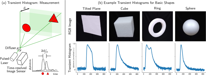
Figure 1: Transient histogram: Measurement and examples. (a) Measuring a transient histogram involves illuminating the scene with a pulsed illumination source such as a pulsed laser which is diffused uniformly over the field of view of a time-resolved image sensor pixel such as a single-photon avalanche diode. (b) Transient histograms were captured using a hardware prototype for some basic 3D shapes. Observe that these have unique features which can help distinguish these shapes.

Vision and robotics systems enabled by 3D cameras are revolutionizing several aspects of our lives via technologies such as robotic surgery, augmented reality, and autonomous navigation. One catalyst behind this revolution is the emergence of depth sensors that can recover the 3D geometry of their surroundings. While a full 3D map may be needed for several applications such as industrial inspection and digital modeling, there are many scenarios where recovering high-resolution 3D geometry is not required. Imagine a robot delivering food on a college campus or a robot arm sorting packages in a warehouse. In these settings, while full 3D perception may be useful for long-term policy design, it is often unnecessary for time-critical tasks such as obstacle avoidance. There is strong evidence that many biological navigation systems such as human drivers [16] do not explicitly recover full 3D geometry for making fast, local decisions such as collision avoidance. For such applications, particularly in resource-constrained scenarios where the vision system is operating under a tight budget (e.g., low-power, low-cost), it is desirable to have weak 3D cameras which recover possibly low-fidelity 3D scene representations, but with low latency and limited power.

We propose a class of weak 3D cameras based on transient histograms, a scene representation tailored for time-critical and resource-constrained applications such as fast robot navigation. A transient histogram is a one-dimensional signal (as opposed to 2D images) that can be captured at high speeds and low-costs by re-purposing cheap proximity sensors that are now ubiquitous, everywhere from consumer electronics such as mobile phones, to cars, factories, and robots for collision safety. Most proximity sensors consist of a laser source and a fast detector and are based on the principle of time-of-flight (ToF): measuring the time it takes for a light pulse to travel to the scene and back to the sensor.

Conventionally, in a ToF sensor, both the fields of view (FoV) of the laser and that of the detector need to coincide and be highly focused (ideally at a single scene point). This ensures that the received light intensity has a single discernible peak corresponding to the round-trip time delay. We adopt a different approach. Instead of focusing the beam on a narrow region, we deliberately diffuse both the laser and the detector so that a large scene area is illuminated simultaneously. The received light is composed of the superposition of all scaled and shifted light pulses from all the illuminated scene points. The resulting captured waveform is called the transient histogram or simply a transient. Instead of encoding the depth of a single scene point, a transient is an aggregate 3D scene representation that encodes information about the 3D geometry and albedos of a large scene patch, possibly even the entire scene.

We propose a family of algorithms that can extract scene information from transients, beyond what is achieved simply via peak-finding. These methods broadly fall under two categories: parametric and non-parametric. For scenes where some prior knowledge can be explicitly modeled, we show an analysis-by-synthesis approach that can be used to recover the scene parameters. While this technique can be used for arbitrary parametric scenes, we show results for planar scenes in Section 4. We demonstrate the viability of plane estimation using a hardware prototype that uses a low-cost, off-the-shelf proximity sensor. Finally, for more complicated scenes, we present a learning-based method in Section 5 to recover a dense depth map using only a small (e.g., $20\times 15$) array of transients. We then show how these depth maps can be further refined using an RGB image, and demonstrate these techniques on a custom hardware setup which is more flexible than a cheap off-the-shelf sensor, yet mimics its characteristics closely.

Scope and Limitations: The proposed techniques are specifically tailored for applications running on resource-constrained devices, where a low-fidelity depth representation suffices. Our methods are not meant to replace conventional depth cameras in scenarios that require dense and high-precision geometry information. Instead, the transient histograms should be considered a complementary scene representation that can be recovered with low latency and compute budgets using only low-cost proximity sensors.

Due to an inherent rotational ambiguity when estimating planes from a single transient, an analytic solution to recover depth of a piecewise planar scene is infeasible. Instead, we adopt a deep learning approach to estimate the geometry of complex scenes. Despite successful demonstration of plane estimation results with a cheap proximity sensor, using SPAD sensors to image more complex scenes is still challenging due to data bandwidth, low signal-to-noise ratio (SNR), and range issues. We instead show depth estimation results using a custom lab setup that was built to perform similarly as off-the-shelf proximity sensors, while providing us with greater flexibility and low-level access to transient histograms.

2 Related Work

3D Imaging Techniques: Traditional depth sensing methods such as stereo, structured-light, and time-of-flight are capable of acquiring high-quality depth maps. While these methods have made significant progress, such as multi-camera depth estimation [39, 35, 40], they still face key challenges. Certain applications such as autonomous drones, cannot support complex structured-light sensors, multiple cameras, or bulky LiDARs due to cost, power, and other constraints. We propose a method suitable for budget-constrained applications which is less resource-intensive because it can estimate depth maps from just a few transients.

Monocular Depth Estimation (MDE): A promising low-cost depth recovery technique is monocular depth estimation which aims to estimate dense depth maps from a single RGB image. Early works on MDE focus on hand-crafted appearance features [12, 13, 33, 32] such as color, position, and texture. Modern MDE techniques use almost exclusively learning-based approaches, including multi-scale deep networks [6, 22], attention mechanisms [11, 1, 14], and recently vision-transformers [30]. Despite predicting ordinal depth well and providing exceptional detail, existing methods cannot resolve the inherent scale ambiguity, resulting in overall low depth accuracy as compared to LiDAR systems.

One possible approach to overcome this ambiguity is to augment the input RGB image with additional information such as the scene’s average depth [41, 2] or a sparse depth map [37, 3]. Some approaches have also designed specialized optics that help disambiguate depth [5, 36]. However, these approaches either require customized hardware that is not readily available or rely on some external information that cannot easily be procured. Sensor fusion techniques like that of Lindell et al. [19] learn to predict depth maps from dense $256\times 256$ ToF measurements and a collocated RGB image. In contrast, our proposed method does not need an RGB image, and yields good results with as few as $4\times 3$ transients, thus saving on power and compute requirements.

Transient-based Scene Recovery: Recently, transient-based depth recovery methods have been proposed, including a two-step process [25] that first uses a pretrained MDE network to predict a rough depth estimate which then gets tuned as its transient gets aligned to match a captured one. This approach relies on the original MDE-based depth map to be ordinally correct for achieving high-quality depths. Further, this two-step method can only work in the presence of a collocated RGB camera. Callenberg et al. [4] use a 2-axis galvo-mirror system with a low-cost proximity sensor to scan the scene. This leads to an impractical acquisition time of more than 30 minutes even for a relatively low $128\times 128$ resolution scan. Our goal is different. We aim to recover 3D scene information from a single transient or a sparse spatial grid (e.g., $20\times 15$) of transients, with minimal acquisition times and computation costs.

Non-Line-of-Sight Imaging (NLOS): NLOS techniques aim to recover hidden geometry using indirect reflections from occluded objects [29, 23, 34, 38]. Instead of diffusing light off a relay surface, our method diffuses the source light in a controlled manner and only captures direct scene reflections. This provides higher SNR, enables use of off-the-shelf detectors, and consumes lower power by estimating depth with orders of magnitude fewer transients than NLOS methods.

3 Transient Histograms

We consider an active imaging system that flash illuminates a large scene area by a periodic pulse train of Dirac delta laser pulses, where each pulse deposits $\Phi_{\text{laser}}$ photons into the scene over a fixed exposure time. The laser light is uniformly diffused over an illumination cone angle $\theta$. In practice, this can be achieved with a diffuser as in Fig. 1(a). Let $f$ denote the repetition frequency of the laser. The unambiguous depth range is given by $r_{\text{max}}=\frac{c}{2f}$ where $c$ is the speed of light.

The imaging system also includes a single-pixel lens-less time-resolved image sensor, co-located with the laser. The sensor collects photons returning from the field of view illuminated by the laser source. Let $\Delta$ be the time resolution of the image sensor pixel, which corresponds to a distance resolution of $\frac{c\Delta}{2}$. The unambiguous depth range $r_{\text{max}}$ is therefore discretized into $N=\lfloor\nicefrac{{1}}{{f\Delta}}\rfloor$ bins.

3.1 Image Formation

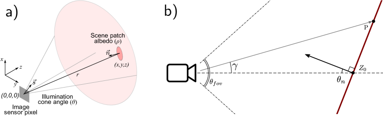
Figure 2: Geometry for radiometric image formation model and planar parametrization. (a) The single-pixel image sensor receives light from a scene patch with albedo $\rho$ located at a distance $r$. The normal vectors at the scene patch and the sensor pixel are denoted by $\vec{n}$ and $\vec{s}$. The transient response at a fixed time delay is computed by integrating the total light returning from all scene patches located in a small range corresponding to the time resolution of the sensor pixel. (b) When viewed in the $(\vec{n},\vec{s})$ plane, the scene plane is parametrized by its distance $Z_{0}$ from the sensor and its angle $\theta_{n}$ measured with respect to sensor’s optical axis.

Fig. 2(a) shows the imaging geometry used for deriving the radiometric image formation model, where a 3D coordinate system is fixed with the single-pixel sensor at the origin and positive $z$-axis pointing into the scene. The laser source is also located at the origin with its direction defined by $\vec{s}$. We assume that the scene is composed of a discrete collection of perfectly Lambertian scene patches. Each visible scene patch has a depth $z$ parametrized by its $(x,y)$ location. Thus, the albedo and surface normal of each patch is given by $\rho(x,y)$ and $\vec{n}(x,y)$. We assume that there are no inter-reflections within the scene and all scene patches that contribute to the signal received by the sensor are inside the unambiguous depth range $0\!\leq\!r\!:=\!\sqrt{x^{2}+y^{2}+[z(x,y)]^{2}}\!<\!r_{\text{max}}=\nicefrac{{c}}{{2f}}.$

The received laser photon flux vector consists of $N$ bins with mean rates given by $\boldsymbol{\varphi}=(\varphi_{1},\varphi_{2},\ldots,\varphi_{N})$. We call $\boldsymbol{\varphi}$ the transient histogram. The photon flux $\varphi_{i}^{\text{laser}}$ contributed by the laser illumination at the $i^{\text{th}}$ bin is given by integrating the light returning from all scene patches that lie in a range of distances satisfying $\nicefrac{{(i-1)c\Delta}}{{2}}\leq r<\nicefrac{{ic\Delta}}{{2}}$. Ignoring multi-bounce paths,

$$\begin{split}\varphi^{\text{laser}}_{i}&=\iint_{(x,y):\frac{(i-1)c\Delta}{2}\leq r<\frac{ic\Delta}{2}}\frac{\rho(x,y)}{4\pi^{2}(1-\cos(\theta_{\text{fov}}/2))r^{4}}(\vec{n}(x,y)\cdot\vec{s})\Phi_{\text{laser}}\,\,dr\\ &=\iint_{(x,y):\frac{(i-1)c\Delta}{2}\leq r<\frac{ic\Delta}{2}}\frac{\hat{\rho}(x,y)}{4\pi^{2}(1-\cos(\theta_{\text{fov}}/2))r^{4}}\Phi_{\text{laser}}\,\,dr\end{split}$$

where $\hat{\rho}$ is the cosine-angle adjusted albedo of the scene patch. Again, $\theta_{\text{fov}}$ is the illumination cone angle, $\vec{n}(x,y)$ is the surface normal of the scene patch, $\vec{s}$ is the source normal and $\Phi_{\text{laser}}$ is the number of photons in each laser pulse.

The final transient histogram at bin $i$ is thus given by:

$$\varphi_{i}=\varphi_{i}^{\text{laser}}+\varphi^{\text{bkg}}$$ (1)

where the constant background component $\varphi^{\text{bkg}}$ consists of the ambient photon flux (e.g., sunlight) and internal sensor noise (e.g., due to dark current). A transient histogram thus forms a scene representation that integrates the effects of scene depth, surface normal, and surface albedo into a one dimensional signal, further affected by ambient light and sensor noise. When measuring a transient histogram, a random number of photons will be incident during each bin $i$ according to a Poisson distribution with mean $\varphi_{i}$.

3.2 Measuring a Transient Histogram

The key strength of a transient histogram is its high temporal resolution. Such a scene representation can be captured using fast detectors that can operate on nano-to-picosecond timescales. One such technology is the avalanche photodiode (APD). APDs equipped with a high-sampling-rate analog-to-digital converter can be used to capture the full transient histogram in a single laser pulse. Our hardware prototypes use a different image sensing technology called single-photon avalanche diode (SPAD). SPADs have gained popularity in recent years due to their single-photon sensitivity and extreme time resolution ($\sim$$100\text{\,}\mathrm{ps}$). Unlike APDs, SPAD arrays can be manufactured cheaply and at scale using standard CMOS fabrication technology.

Estimating Transient Histograms using SPADs: Unlike a conventional image sensor, a SPAD pixel can capture at most one returning photon per laser period. This is because, after each photon detection event, the SPAD pixel enters a dead-time during which the pixel is reset. Conventionally, a SPAD pixel is operated in synchronization with the pulsed laser; photon timestamps are acquired over many laser cycles, and a histogram of photon counts is constructed. We call this the SPAD histogram. We now show that the scene’s transient histogram can be estimated from a measured SPAD histogram.

In each laser cycle, the probability $q_{i}$ that at least one photon is incident on the SPAD pixel in bin $i$ can be calculated using Poisson statistics: $q_{i}\!=\!1\!-\!e^{-\varphi_{i}}$. The probability $p_{i}$ that the SPAD captures a photon in the $i^{\text{th}}$ bin follows a geometric distribution: $p_{i}=q_{i}\prod_{j<i}q_{j}$. For convenience, the $(N\!+\!1)^{\text{th}}$ SPAD histogram bin stores the number of laser cycles with no photon detection: $p_{N+1}=1-\sum_{i=1}^{N}p_{i}$. If the total incident photon flux is low such that only a small fraction of the laser cycles lead to a photon detection, the expected number of photons measured by the SPAD in bin $1\leq i\leq N$ is proportional to the transient histogram: $\mathbf{E}[h_{i}]=L\varphi_{i}$ where $L$ is the number of laser cycles. The transient histogram is thus $\widetilde{\varphi}_{i}=\nicefrac{{h_{i}}}{{L}}$. We assume that the SPAD pixel captures 512 bins over a $10\text{\,}\mathrm{m}$ range corresponding to a time bin resolution of $130\text{\,}\mathrm{ps}$.

3.3 Information in a Transient Histogram

A key question arises: “What information does a transient histogram contain?”. Fig. 1(b) shows example histograms for simple shapes, captured experimentally. These histograms have unique features for different shapes. Each histogram has a sharp leading edge corresponding to the shortest distance from the sensor to the object. For a 2D tilted plane, the transient histogram also has a sharp trailing edge with a drop-off to zero. The support (width of the non-zero region) reveals the difference between the farthest and the nearest visible point on the object. For 3D shapes like the cube and the sphere, there is no sharp trailing edge, and the drop-off is more gradual. The 3D ring has a double peak, the distance between these peaks is a function of the angle of the plane of the ring with respect to the sensor.

While the leading edge of a transient histogram gives an accurate estimate of the distance to the nearest point on an object, recovering the depth map $z(x,y)$ from a histogram is severely under-determined even for very simple shapes, as a transient histogram is an integration of depth, surface normal and albedo. Physically plausible scenes with different depth maps can produce the same transient histogram.

• Albedo-depth ambiguity: A peak’s height conflates radiometric fall-off and albedo. A small highly reflective (high albedo) object at a given distance will produce an equally strong peak as a larger but more diffuse object.

• Albedo-normal ambiguity: Both a tilted scene patch, and a patch with low albedo will reflect less light than a head-on, high albedo one.

• Orientation ambiguity: The transient histogram is insensitive to rotational symmetry; a plane tilted at $45\text{\,}\mathrm{\SIUnitSymbolDegree}$ clockwise or counterclockwise with respect to the $x-y$ plane will produce exactly the same transient histogram.

We now present a family of techniques to recover 3D scene information from transient histograms, beyond what can be achieved via simple peak-finding.

4 Plane Estimation with Transient Histograms

As pointed out by previous works [21, 20, 18], numerous scenes especially indoor ones can be well approximated as piecewise planar. Here, we study the problem of recovering the parameters of a planar scene from a captured transient. By limiting ourselves to estimating a single plane per transient, we simplify the problem without loss of generality: one could apply our method to a small array of transients to estimate a piecewise planar scene. Solving this problem will provide insights on estimating more complex 3D geometry e.g., piecewise planar scenes, and other parametric shapes.

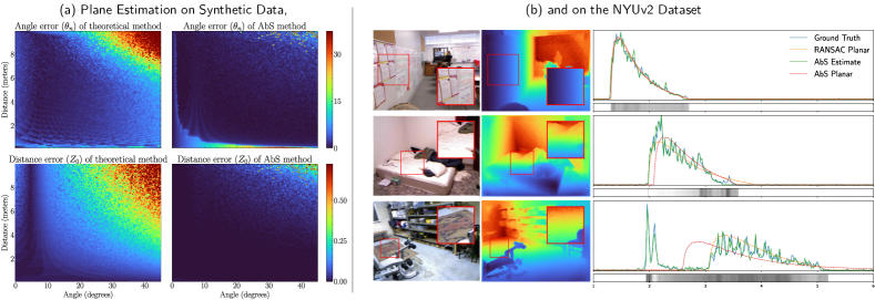
Figure 3: Plane Estimation on Synthetic and NYUv2 data. (a) We evaluate the mean average error of estimated plane parameters produced by each approach over a wide range of parameter combinations. The first column corresponds to the theoretical approach, the second is the analysis by synthesis approach. (b) We show a few NYUv2 patches and their accompanying transients. Solid transients represent the simulated ground truth (blue) and the resulting transient produced by the AbS method (green). Dashed transients correspond to what we would observe if the scene was perfectly planar with uniform albedo with parameters as estimated by the RANSAC fitting process (orange), and with parameters estimated by the AbS approach (red). Below each transient, we show the average albedo per bin.

Plane Parametrization: We parameterize a plane by its normal as given in spherical coordinates $\vec{n}=[1,\theta_{n},\phi_{n}]^{\intercal}$, and the distance $Z_{0}$, at which the plane intercepts the sensor’s optical axis (Fig. 2(b)). Due to rotational symmetry, it is not possible to recover the azimuth $\phi_{n}$, so we focus on estimating $\theta_{n}$ and $Z_{0}$.

4.1 Plane Estimation Algorithms

Theoretical Estimator: For small FoVs, $Z_{0}$ can be directly estimated by finding the location of the largest peak in the transient. This estimator becomes less accurate as the FoV increases, but in practice, this decay can be neglected, or a better estimate can be derived from the center of the transient’s support if necessary. To estimate $\theta_{n}$, we refer to Fig. 2(b). The distance to a point on the plane $P$ at a viewing angle $\gamma$, as measured from the optical axis, is given by:

$$||P||=Z_{0}\frac{\cos{\left(\theta_{n}\right)}}{\cos{\left(\gamma+\theta_{n}\right)}}.$$ (2)

With the exception of when $\theta_{n}$ is zero, Eq. (2) reaches its extrema at $\pm\theta_{\text{fov}}/2$, corresponding to the furthest and closest visible scene points, respectively. These extrema can be directly estimated from the transient by detecting the leading and lagging edges of the peak from the 1D signal. This yields two new distances denoted $D_{1},D_{2}$, which each gives an estimate of $\theta_{n}$ by Eq. (2). Averaging these two estimates yields our final estimate for $\theta_{n}$. While such an estimator only relies on basic peak finding primitives, it may fail for large values of $Z_{0}$ and $\theta_{n}$ when the lagging edge of the peak falls outside the unambiguous depth range.

Analysis-by-Synthesis Algorithm: We introduce an analysis-by-synthesis (AbS) based estimator that further refines the theoretical estimator. The key idea is to directly optimize the scene parameters ($\theta_{n},Z_{0}$) using a differentiable forward rendering model $R(\theta_{n},Z_{0})$ that approximates the image formation defined in Eq. (1). This is done by discretizing the integral and replacing the transient binning operation with a soft-binning process which uses a sharp Gaussian kernel for binning. Specifically, given a measured transient histogram $\widetilde{\varphi}=\{\widetilde{\varphi}_{i}\}_{i=1}^{N}$, we solve the following optimization problem using gradient descent, with the initial solution of $\theta_{n}$ and $Z_{0}$ given by our theoretical approach:

$$\underset{\theta_{n},Z_{0}}{\operatorname*{arg\,min}}\ ||\mathcal{F}\left(R(\theta_{n},Z_{0})\right)-\mathcal{F}\left(\widetilde{\varphi}\right)||^{2}_{2}$$ (3)

where $\mathcal{F}$ denotes the Fourier transform. The $\mathcal{L}_{2}$ norm is computed on the top $k=64$ of the $512$ complex-valued Fourier coefficients. This is equivalent to low-pass filtering the signal and removes high-frequency noise. Please see the supplement for details.

4.2 Simulation Results

Quantitative Results on Synthetic Data: To evaluate the effectiveness of our approaches, we simulated transients that correspond to uniform-albedo planes with $Z_{0}\in[0,10]$ meters and $\theta_{n}\in[0,45]$ degrees. For each transient, we estimated plane parameters with the theoretical and AbS methods and compare these to the ground truth. Results can be found in Fig. 3(a). We observe that the AbS method performs better than the theoretical method $87\%$ of the time for estimating $\theta_{n}$ and $97\%$ for $Z_{0}$.

Simulating Transients with RGB-D Data: We assume a Lambertian scene and simulate transients produced under direct illumination using paired RGB images and depth maps from existing RGB-D datasets. A ground truth transient histogram is generated through Monte Carlo integration for each scene. We sample rays emitted by the light source, march them until they intersect a scene surface, and weight the returning signal by scene albedo.

Qualitative Results on NYUv2 Dataset: We further test our methods on images from NYUv2 [24] — a well-known RGB-D dataset. Transient histograms of local patches were simulated, and plane fitting using RANSAC was performed on the depth map to estimate surface normals of the patches. Results of our methods with simulated transients as inputs were compared against estimated surface normals, as shown in Fig. 3(b).

4.3 Hardware Prototype and Results

We built a low-cost hardware prototype using a SPAD-based proximity sensor (AMS TMF8801, retail price $\sim$2 USD) and a Raspberry Pi Zero W mounted on a custom 3D printed mount. This sensor has a bin resolution of $200\text{\,}\mathrm{p}\mathrm{s}$ and a FoV of $\sim$20 degrees. As shown in Fig. 4(a) the sensor is attached to a plywood structure and scans a test plane from different angles controlled using a servo motor. The sensor and test plane are at a known distance apart. We recover the plane angle $\theta_{n}$ from the transient histograms. Using the servo to rotate the styrofoam backplate to all angles within $[-60^{\circ},60^{\circ}]$ in increments of $1^{\circ}$, we acquired 100 transients at each angle and with each of the 6 textures shown in Fig. 4(b). We capture this range to acquire more data and correct miscalibrations.

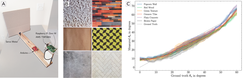
Figure 4: Hardware prototype for plane estimation and results. (a) Our low-cost prototype consists of an AMS TMF8801 sensor that scans a planar scene from different angles. (b) We captured data from a variety of plane textures and albedos. (c) Our method successfully estimates plane parameters for a wide range of plane textures.

Results: Fig. 4(c) shows the mean $\theta_{n}$ estimate, as well as the standard deviation, for each of the six textures. In line with the simulation results shown in Fig. 3(a), our theoretical approach gives reliable estimates with experimental data over a wide range of angles. The estimates are inaccurate when $\theta_{n}$ is small (e.g., $\leq 5^{\circ}$). Although our theoretical model assumes a Lambertian plane, in practice this method is robust to real-world albedo variations and provides reliable estimates even with non-Lambertian textured surfaces.

5 Depth Estimation via Transient Histograms

We now consider estimating depth for scenes with complex geometry and albedos. Due to the inherent rotational ambiguity of our plane estimation method, it is challenging to extend it to a small array of transient and model the scene as piecewise planar. While it is possible to estimate the remaining $\phi_{n}$ parameters from spatially-neighboring transients this method does not generalize well to more complex scenes, especially if they violate local planar assumptions. To accomplish this task without prior knowledge of the scene’s overall shape we design a deep model to predict dense depth from a sparse set of transient histograms. We also demonstrate that the resulting depth map can be further refined with an additional RGB input image.

Multiple Transients: Recovering complex geometry from a single transient histogram is a severely ill-posed problem. So we propose to use a low spatial resolution 2D array of defocused SPAD pixels that image sub-regions of the complete FoV. Two configurations are considered: a $4\times 3$ array of SPADs, each with a FoV of 25 degrees, and a $20\times 15$ array each with a FoV of 10 degrees. The specific fields of view are chosen to cover the whole scene with each SPAD’s FoV overlapping slightly with its neighbors. For an output resolution of $640\times 480$, these arrays correspond to a downsampling ratio of $160\times$ and $32\times$ respectively.

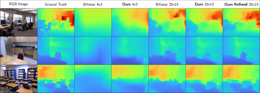
Figure 5: Simulated Results on NYUv2 Dataset. From left to right this figure shows the RGB image, ground truth depth, bilinear upsampling followed by our method using the $4\times 3$ tiling, bilinear upsampling followed by our method using the $20\times 15$ tiling, and finally the refined results for the $20\times 15$ grid. See supplement for more results.

5.1 Scene Depth from Transients via Deep Models

We now describe deep models for estimating depth from transient histograms and for refining the depth map with the guidance of an RGB image.

Depth Estimation: We adapt a deep convolutional neural network architecture similar to that of recent monocular depth estimation methods [8] to perform depth estimation. The model consists of repeating blocks of convolutional layers and upsampling layers which are stacked until the desired output resolution is achieved. Similar to our previous experiment on plane estimation, we compute the Fourier transform of the input transients and only keep the $k$ coefficients with lowest frequency. We use $k=4$ for the $4\times 3$ grid and $k=16$ for the $20\times 15$ grid. We train the network using the reverse Hubert “BerHu” loss [27, 42]. Details about our models and training procedures are given in the supplement.

Depth Refinement: Estimating depth from a sparse set of SPAD sensors is challenging due to the low spatial resolution. In many cases, we might have access to an RGB image of the scene which contains high-frequency spatial information that is lacking in the transients. It can be used to refine our depth prediction. To accomplish this, we combine two existing methods. The first, FDKN [15] is trained to refine a low-resolution depth map given an RGB image. The model was designed to super-resolve a depth map by at most $16\times$, beyond which there is significant performance degradation. Directly using this network as a post-processing step helps yet leads to noticeable artifacts even when finetuned. To alleviate this we use the pre-trained DPT [30] model. Despite its low absolute depth accuracy, DPT provides high-resolution spatial details.

Specifically, the depth map produced by the FDKN network is used as a guidance image which determines how the depth map from DPT should be deformed. On a tile-by-tile basis, we compute the scale and shift that minimizes the $\mathcal{L}_{2}$ loss between the two depth maps. Once this transformation is interpolated over the whole depth map and applied to the DPT prediction, we get our final result: a depth map with greater spatial detail and higher accuracy than MDE.

Table 1: Results on NYUv2 Benchmark. We show numerical results for our approaches, baselines, and well-known MDE methods. While MDE approaches can produce detailed depth maps, their absolute depth accuracy (in the lower $\delta$ metrics) is at par with our $4\times 3$ grid. Our approach produces more accurate depth maps overall.

Grid Size	Method	$\delta<1.05^{1}\uparrow$	$\delta<1.05^{2}\uparrow$	$\delta<1.05^{3}\uparrow$	$\delta<1.25^{1}\uparrow$	$\delta<1.25^{2}\uparrow$	$\delta<1.25^{3}\uparrow$	$Log_{10}\downarrow$		$AbsRel\downarrow$	$RMSE\downarrow$
$4\times 3$	Ours	0.335	0.577	0.724	0.845	0.953	0.981	0.068		0.126	0.604
	Baseline	0.340	0.569	0.709	0.824	0.934	0.967	0.171		0.147	0.652
	Bilinear	0.285	0.466	0.588	0.715	0.886	0.951	0.083		0.169	0.856
$20\times 15$	Ours	0.624	0.809	0.880	0.929	0.976	0.989	0.060		0.073	0.409
	Baseline	0.576	0.786	0.867	0.923	0.973	0.988	0.066		0.084	0.450
	Bilinear	0.583	0.763	0.840	0.899	0.963	0.985	0.038		0.081	0.498
	Ours Refined	0.707	0.865	0.924	0.961	0.990	0.996	0.024		0.053	0.287
MDE	DORN [9]	0.394	0.602	0.731	0.846	0.954	0.983	0.053		0.120	0.501
	DenseDepth [2]	0.311	0.548	0.706	0.847	0.973	0.994	0.053		0.123	0.461
	BTS-DenseNet [17]	0.357	0.607	0.764	0.885	0.978	0.994	0.047		0.110	0.392
	DPT [30]	0.326	0.595	0.767	0.904	0.988	0.998	0.045		0.109	0.357

5.2 Simulation Results

Dataset: We use the standard test/train split of the widely used NYUv2 dataset [24] which is a large indoor dataset with dense ground truths.

Evaluation Metrics: To quantitatively evaluate our results, we compare our approach to existing methods using the standard metrics used in prior work [7], including Absolute Relative Error (AbsRel), Root Mean Squared Error (RMSE), Average Log Error (Log10), and Threshold Accuracy ($\delta<thr$). See supplement.

Existing literature focuses on $\{1.25,1.25^{2},1.25^{3}\}$ thresholds that correspond to $25\%$, $56\%$, and $95\%$ depth error. However, we believe that many real world applications such as robot navigation and obstacle avoidance need stronger accuracy guarantees. To better quantify the gap between LiDARs and MDE-based methods, we consider three stricter thresholds $\{1.05,1.05^{2},1.05^{3}\}$ that correspond to $5\%$, $10\%$ and $16\%$ error.

Baselines: A simple baseline uses bilinear upsampling of the tiled depth as computed via peak-finding. We also consider a stronger baseline that uses a deep network to super-resolve depth maps at each tile. We compare with recent MDE methods [9, 2, 17, 30] for which some metrics were re-computed using the pre-trained models as these were not published in the original papers.

Qualitative Results: Fig. 5 compares our method against various baselines. Observe that in the first and last rows, our network can extract more information from a transient: farther scene depths that are missing in a bilinear-upsampled depth maps are visible with our method. This effect is particularly noticeable for the smaller $4\times 3$ grid. The last column shows results of our depth-refinement method which adds more spatial details.

Quantitative Results: Table 1 presents our main results. As seen in the lower $\delta$ metrics, our method provides the most benefits using small grids. We observe a $5\%$ accuracy increase over bilinear in the lowest $\delta$ metric for the small grid whereas it only boosts it by $4.1\%$ in the larger grid. Moreover, observe that our refinement step increases the $5\%$-accuracy metric by more than $8\%$, and reaches nearly double the accuracy of some MDE approaches.

Energy, latency, and cost: Table 2 shows a comparison of our method ($4\times 3$) using a (simulated) low-cost SPAD vs. a conventional RGB camera in terms of power consumption, bandwidth, compute cost, and depth accuracy. Our method generates similar depth quality as MDE approaches while consuming $\nicefrac{{1}}{{10}}^{\text{th}}$ the power, 2400$\times$ less bandwidth, and orders of magnitude less compute. We expect such low-resolution ($4\times 3$) SPAD arrays will be significantly cheaper than high resolution RGB and ToF camera modules. Table 2 does not include the optional RGB refinement step which will consume additional resources.

Table 2: Sensing power and compute costs. Power estimates are based on an AMS TMF8828 proximity sensor and a typical smartphone camera. Timing analysis is conducted on an Intel Core i7-9700K CPU and Nvidia RTX 2080 SUPER GPU with an input resolution of $640\times 480$ and averaged over 300 runs.

Method	Peak Power	Bandwidth	GFLOPS	#Params	Time	$\delta<1.25^{3}\uparrow$
Ours $4\times 3$	$141$ mW	$384$ B	$0.811$	$28.6$ K	$2.77$ ms	$0.981$
DORN [9]	$1.98$ W	$900$ kB	$389.5$	$162.7$ M	$112.0$ ms	$0.983$
DPT [30]	$1.98$ W	$900$ kB	$280.3$	$120.7$ M	$81.4$ ms	$0.998$

5.3 Hardware Prototype and Experiment Results

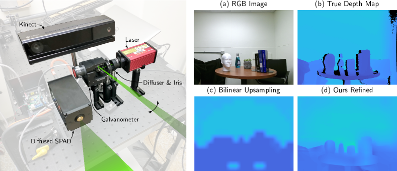
Figure 6: Hardware prototype and experiment results. Our hardware prototype (left) scans a $20\times 15$ grid in the scene with a diffused laser spot. A lens-less SPAD pixel captures transient histograms. (a) We imaged a table-top scene with a wide range of albedos and textured objects. (b) The true depth map captured using a Kinect v2. (c) Simple peak-finding-based depth map provides no depth details. (d) Using the RGB image and an MDE model, our method generates a higher resolution depth map.

Our lab cart hardware prototype (Fig. 6) was designed to be similar in operation to a low-cost off-the-shelf AMS TMF8828 proximity sensor. However, this setup provides greater flexibility with reprogramming and alignment with the RGB-D camera, and allows evaluating different scanning patterns. Our setup consists of a pulsed laser (Thorlabs NPL52C) with a $6\text{\,}\mathrm{ns}$ pulse width, $1.2\text{\,}\mathrm{W}$ peak power, and $40\text{\,}\mathrm{kHz}$ repetition frequency. The laser spot is diffused and shaped into a $10\text{\,}\mathrm{\SIUnitSymbolDegree}$ cone using a diffuser (Thorlabs ED1-C20) and an adjustable circular iris. The detector is a lens-less single-pixel SPAD (MPD InGaAs Fast Gated SPAD) operated in gated acquisition mode with a dead-time of $1\text{\,}\mathrm{\SIUnitSymbolMicro s}$. The FoV of the SPAD pixel covers the whole scene. A 2-axis galvanometer (Thorlabs GVS012) scans a $20\times 15$ grid that covers the FoV. In practice, this can be replaced with a low-resolution multi-pixel SPAD array. Photon timestamps are acquired using a time-correlated single-photon counting (TCSPC) system and histograms are constructed offline. A Microsoft Kinect v2 RGB-D camera provides ground truth intensity and depth maps.

Results: Fig. 6 (right panel) also shows results on an indoor table-top scene using our setup. This scene is challenging due to several objects with varying reflectances and sharp depth edges. Using bilinear upsampling from the transient peaks results in jagged edges and overall loss of detail. The proposed methods can recover fine details and accurate depths with as few as $20\times 15$ transients. For more results and comparisons, please refer to the supplementary material.

6 Limitations and Discussion

Bottlenecks and Availability: Proximity sensors containing small arrays of SPAD pixels are already commonplace in consumer electronics. However, they only output a single depth measurement. Some off-the-shelf sensors provide limited access to low-resolution pre-processed transients. Bandwidth bottlenecks between the sensor and processing unit limit the rate at which transients can be read out. For the methods described in this paper to become widespread, sensor manufacturers need to address communication bottlenecks, and document and advertise low-level APIs that allow direct access to transients.

Future Outlook: Faster communication protocols and on-chip compression methods will enable capturing transient histograms at high frame rates using commodity hardware. These can not only be used to determine scene geometry but also help resolve objects in low-light, detect fast-moving targets, and detect subtle scene motion (e.g. heartbeat or acoustic vibrations). Transient histograms can be treated as a primitive scene representation complementary to RGB images for time-critical and resource-constrained applications.

Acknowledgments: This research was supported in part by the NSF CAREER award 1943149, NSF award CNS-2107060 and Intel-NSF award CNS-2003129. We thank Talha Sultan for help with data acquisition.

References

- [1] Aich, S., Vianney, J.M.U., Islam, M.A., Kaur, M., Liu, B.: Bidirectional Attention Network for Monocular Depth Estimation. arXiv:2009.00743 [cs] (Sep 2020), http://arxiv.org/abs/2009.00743, arXiv: 2009.00743
- [2] Alhashim, I., Wonka, P.: High Quality Monocular Depth Estimation via Transfer Learning. arXiv:1812.11941 [cs] (Mar 2019), http://arxiv.org/abs/1812.11941, arXiv: 1812.11941 version: 2
- [3] Bergman, A.W., Lindell, D.B., Wetzstein, G.: Deep Adaptive LiDAR: End-to-end Optimization of Sampling and Depth Completion at Low Sampling Rates. In: 2020 IEEE International Conference on Computational Photography (ICCP). pp. 1–11. IEEE, Saint Louis, MO, USA (Apr 2020). https://doi.org/10.1109/ICCP48838.2020.9105252, https://ieeexplore.ieee.org/document/9105252/
- [4] Callenberg, C., Shi, Z., Heide, F., Hullin, M.B.: Low-cost SPAD sensing for non-line-of-sight tracking, material classification and depth imaging. ACM Transactions on Graphics 40(4), 1–12 (Aug 2021). https://doi.org/10.1145/3450626.3459824, https://dl.acm.org/doi/10.1145/3450626.3459824
- [5] Chang, J., Wetzstein, G.: Deep Optics for Monocular Depth Estimation and 3D Object Detection. arXiv:1904.08601 [cs, eess] (Apr 2019), http://arxiv.org/abs/1904.08601, arXiv: 1904.08601
- [6] Eigen, D., Fergus, R.: Predicting Depth, Surface Normals and Semantic Labels with a Common Multi-Scale Convolutional Architecture. arXiv:1411.4734 [cs] (Dec 2015), http://arxiv.org/abs/1411.4734, arXiv: 1411.4734
- [7] Eigen, D., Puhrsch, C., Fergus, R.: Depth map prediction from a single image using a multi-scale deep network. In: Proceedings of the 27th International Conference on Neural Information Processing Systems - Volume 2. pp. 2366–2374. NIPS’14, MIT Press, Cambridge, MA, USA (Dec 2014)
- [8] Fang, Z., Chen, X., Chen, Y., Van Gool, L.: Towards Good Practice for CNN-Based Monocular Depth Estimation. In: 2020 IEEE Winter Conference on Applications of Computer Vision (WACV). pp. 1080–1089. IEEE, Snowmass Village, CO, USA (Mar 2020). https://doi.org/10.1109/WACV45572.2020.9093334, https://ieeexplore.ieee.org/document/9093334/
- [9] Fu, H., Gong, M., Wang, C., Batmanghelich, K., Tao, D.: Deep Ordinal Regression Network for Monocular Depth Estimation. CoRR abs/1806.02446 (2018), http://arxiv.org/abs/1806.02446, _eprint: 1806.02446
- [10] Gupta, A., Ingle, A., Gupta, M.: Asynchronous Single-Photon 3D Imaging. In: 2019 IEEE/CVF International Conference on Computer Vision (ICCV). pp. 7908–7917. IEEE, Seoul, Korea (South) (Oct 2019). https://doi.org/10.1109/ICCV.2019.00800, https://ieeexplore.ieee.org/document/9009520/
- [11] Hao, Z., Li, Y., You, S., Lu, F.: Detail Preserving Depth Estimation from a Single Image Using Attention Guided Networks. arXiv:1809.00646 [cs] (Sep 2018), http://arxiv.org/abs/1809.00646, arXiv: 1809.00646
- [12] Hoiem, D., Efros, A.A., Hebert, M.: Automatic photo pop-up. In: ACM SIGGRAPH 2005 Papers. pp. 577–584. SIGGRAPH ’05, Association for Computing Machinery, New York, NY, USA (Jul 2005). https://doi.org/10.1145/1186822.1073232, https://doi.org/10.1145/1186822.1073232
- [13] Hoiem, D., Efros, A.A., Hebert, M.: Recovering Surface Layout from an Image. International Journal of Computer Vision 75(1), 151–172 (Jul 2007). https://doi.org/10.1007/s11263-006-0031-y, http://link.springer.com/10.1007/s11263-006-0031-y
- [14] Huynh, L., Nguyen-Ha, P., Matas, J., Rahtu, E., Heikkila, J.: Guiding Monocular Depth Estimation Using Depth-Attention Volume. arXiv:2004.02760 [cs] (Aug 2020), http://arxiv.org/abs/2004.02760, arXiv: 2004.02760
- [15] Kim, B., Ponce, J., Ham, B.: Deformable Kernel Networks for Joint Image Filtering. International Journal of Computer Vision 129(2), 579–600 (Feb 2021). https://doi.org/10.1007/s11263-020-01386-z, http://arxiv.org/abs/1910.08373, arXiv: 1910.08373
- [16] Lee, D.N.: A theory of visual control of braking based on information about time-to-collision. Perception 5(4), 437–459 (1976). https://doi.org/10.1068/p050437
- [17] Lee, J.H., Han, M.K., Ko, D.W., Suh, I.H.: From Big to Small: Multi-Scale Local Planar Guidance for Monocular Depth Estimation. arXiv:1907.10326 [cs] (Mar 2020), http://arxiv.org/abs/1907.10326, arXiv: 1907.10326 version: 5
- [18] Lee, J., Gupta, M.: Blocks-World Cameras. In: 2021 IEEE/CVF Conference on Computer Vision and Pattern Recognition (CVPR). pp. 11407–11417. IEEE, Nashville, TN, USA (Jun 2021). https://doi.org/10.1109/CVPR46437.2021.01125, https://ieeexplore.ieee.org/document/9578739/
- [19] Lindell, D.B., O’Toole, M., Wetzstein, G.: Single-photon 3D imaging with deep sensor fusion. ACM Transactions on Graphics 37(4), 113:1–113:12 (Jul 2018). https://doi.org/10.1145/3197517.3201316, https://doi.org/10.1145/3197517.3201316
- [20] Liu, C., Kim, K., Gu, J., Furukawa, Y., Kautz, J.: PlaneRCNN: 3D Plane Detection and Reconstruction from a Single Image. arXiv:1812.04072 [cs] (Jan 2019), http://arxiv.org/abs/1812.04072, arXiv: 1812.04072
- [21] Liu, C., Yang, J., Ceylan, D., Yumer, E., Furukawa, Y.: PlaneNet: Piece-wise Planar Reconstruction from a Single RGB Image. arXiv:1804.06278 [cs] (Apr 2018), http://arxiv.org/abs/1804.06278, arXiv: 1804.06278 version: 1
- [22] Liu, F., Shen, C., Lin, G., Reid, I.: Learning Depth from Single Monocular Images Using Deep Convolutional Neural Fields. IEEE Transactions on Pattern Analysis and Machine Intelligence 38(10), 2024–2039 (Oct 2016). https://doi.org/10.1109/TPAMI.2015.2505283, http://arxiv.org/abs/1502.07411, arXiv: 1502.07411
- [23] Metzler, C.A., Lindell, D.B., Wetzstein, G.: Keyhole Imaging: Non-Line-of-Sight Imaging and Tracking of Moving Objects Along a Single Optical Path. IEEE Transactions on Computational Imaging 7, 1–12 (2021). https://doi.org/10.1109/TCI.2020.3046472, conference Name: IEEE Transactions on Computational Imaging
- [24] Nathan Silberman, Derek Hoiem, P.K., Fergus, R.: Indoor Segmentation and Support Inference from RGBD Images. In: ECCV (2012)
- [25] Nishimura, M., Lindell, D.B., Metzler, C., Wetzstein, G.: Disambiguating Monocular Depth Estimation with a Single Transient. European Conference on Computer Vision (ECCV) (2020)
- [26] O’Toole, M., Heide, F., Lindell, D.B., Zang, K., Diamond, S., Wetzstein, G.: Reconstructing Transient Images from Single-Photon Sensors. In: 2017 IEEE Conference on Computer Vision and Pattern Recognition (CVPR). pp. 2289–2297 (Jul 2017). https://doi.org/10.1109/CVPR.2017.246, iSSN: 1063-6919
- [27] Owen, A.B.: A robust hybrid of lasso and ridge regression. In: Verducci, J.S., Shen, X., Lafferty, J. (eds.) Contemporary Mathematics, vol. 443, pp. 59–71. American Mathematical Society, Providence, Rhode Island (2007). https://doi.org/10.1090/conm/443/08555, http://www.ams.org/conm/443/
- [28] Pediredla, A.K., Sankaranarayanan, A.C., Buttafava, M., Tosi, A., Veeraraghavan, A.: Signal Processing Based Pile-up Compensation for Gated Single-Photon Avalanche Diodes. arXiv:1806.07437 [physics] (Jun 2018), http://arxiv.org/abs/1806.07437, arXiv: 1806.07437
- [29] Pediredla, A.K., Buttafava, M., Tosi, A., Cossairt, O., Veeraraghavan, A.: Reconstructing rooms using photon echoes: A plane based model and reconstruction algorithm for looking around the corner. In: 2017 IEEE International Conference on Computational Photography (ICCP). pp. 1–12 (May 2017). https://doi.org/10.1109/ICCPHOT.2017.7951478, iSSN: 2472-7636
- [30] Ranftl, R., Bochkovskiy, A., Koltun, V.: Vision Transformers for Dense Prediction. arXiv:2103.13413 [cs] (Mar 2021), http://arxiv.org/abs/2103.13413, arXiv: 2103.13413
- [31] Rapp, J., Rapp, J., Ma, Y., Dawson, R.M.A., Goyal, V.K.: High-flux single-photon lidar. Optica 8(1), 30–39 (Jan 2021). https://doi.org/10.1364/OPTICA.403190, https://opg.optica.org/optica/abstract.cfm?uri=optica-8-1-30, publisher: Optica Publishing Group
- [32] Saxena, A., Sun, M., Ng, A.Y.: Make3D: Learning 3D Scene Structure from a Single Still Image. IEEE Transactions on Pattern Analysis and Machine Intelligence 31(5), 824–840 (2009)
- [33] Saxena, A., Chung, S.H., Ng, A.Y.: Learning depth from single monocular images. In: Proceedings of the 18th International Conference on Neural Information Processing Systems. pp. 1161–1168. NIPS’05, MIT Press, Cambridge, MA, USA (Dec 2005)
- [34] Tsai, C.Y., Kutulakos, K.N., Narasimhan, S.G., Sankaranarayanan, A.C.: The Geometry of First-Returning Photons for Non-Line-of-Sight Imaging. In: 2017 IEEE Conference on Computer Vision and Pattern Recognition (CVPR). pp. 2336–2344 (Jul 2017). https://doi.org/10.1109/CVPR.2017.251, iSSN: 1063-6919
- [35] Wang, Y., Chao, W.L., Garg, D., Hariharan, B., Campbell, M., Weinberger, K.Q.: Pseudo-LiDAR from Visual Depth Estimation: Bridging the Gap in 3D Object Detection for Autonomous Driving. arXiv:1812.07179 [cs] (Feb 2020), http://arxiv.org/abs/1812.07179, arXiv: 1812.07179
- [36] Wu, Y., Boominathan, V., Chen, H., Sankaranarayanan, A., Veeraraghavan, A.: PhaseCam3D — Learning Phase Masks for Passive Single View Depth Estimation. In: 2019 IEEE International Conference on Computational Photography (ICCP). pp. 1–12 (May 2019). https://doi.org/10.1109/ICCPHOT.2019.8747330, iSSN: 2472-7636
- [37] Xia, Z., Sullivan, P., Chakrabarti, A.: Generating and Exploiting Probabilistic Monocular Depth Estimates. arXiv:1906.05739 [cs] (Dec 2019), http://arxiv.org/abs/1906.05739, arXiv: 1906.05739
- [38] Xin, S., Nousias, S., Kutulakos, K.N., Sankaranarayanan, A.C., Narasimhan, S.G., Gkioulekas, I.: A Theory of Fermat Paths for Non-Line-Of-Sight Shape Reconstruction. In: 2019 IEEE/CVF Conference on Computer Vision and Pattern Recognition (CVPR). pp. 6793–6802. IEEE, Long Beach, CA, USA (Jun 2019). https://doi.org/10.1109/CVPR.2019.00696, https://ieeexplore.ieee.org/document/8954312/
- [39] Zhang, F., Qi, X., Yang, R., Prisacariu, V., Wah, B., Torr, P.: Domain-invariant Stereo Matching Networks. arXiv:1911.13287 [cs] (Nov 2019), http://arxiv.org/abs/1911.13287, arXiv: 1911.13287
- [40] Zhang, K., Xie, J., Snavely, N., Chen, Q.: Depth Sensing Beyond LiDAR Range. arXiv:2004.03048 [cs] (Apr 2020), http://arxiv.org/abs/2004.03048, arXiv: 2004.03048
- [41] Zhou, T., Brown, M., Snavely, N., Lowe, D.G.: Unsupervised Learning of Depth and Ego-Motion from Video. In: 2017 IEEE Conference on Computer Vision and Pattern Recognition (CVPR). pp. 6612–6619. IEEE, Honolulu, HI (Jul 2017). https://doi.org/10.1109/CVPR.2017.700, http://ieeexplore.ieee.org/document/8100183/
- [42] Zwald, L., Lambert-Lacroix, S.: The BerHu penalty and the grouped effect. arXiv:1207.6868 [math, stat] (Jul 2012), http://arxiv.org/abs/1207.6868, arXiv: 1207.6868