Clinical Contrastive Learning for Biomarker Detection

Abstract

This paper presents a novel positive and negative set selection strategy for contrastive learning of medical images based on labels that can be extracted from clinical data. In the medical field, there exists a variety of labels for data that serve different purposes at different stages of a diagnostic and treatment process. Clinical labels and biomarker labels are two examples. In general, clinical labels are easier to obtain in larger quantities because they are regularly collected during routine clinical care, while biomarker labels require expert analysis and interpretation to obtain. Within the field of ophthalmology, previous work has shown that clinical values exhibit correlations with biomarker structures that manifest within optical coherence tomography (OCT) scans. We exploit this relationship between clinical and biomarker data to improve performance for biomarker classification. This is accomplished by leveraging the larger amount of clinical data as pseudo-labels for our data without biomarker labels in order to choose positive and negative instances for training a backbone network with a supervised contrastive loss. In this way, a backbone network learns a representation space that aligns with the clinical data distribution available. Afterwards, we fine-tune the network trained in this manner with the smaller amount of biomarker labeled data with a cross-entropy loss in order to classify these key indicators of disease directly from OCT scans. Our method is shown to outperform state of the art self-supervised methods by as much as 5% in terms of accuracy on individual biomarker detection.

Introduction

Contrastive learning [1] refers to a family of self-supervision algorithms that utilize embedding enforcement losses with the goal of training a model to learn a rich representation space. The general premise is that the model is taught an embedding space where similar pairs of images (positives) project closer together and dissimilar pairs of images (negatives) project apart. In order to do this in an unsupervised fashion, modern methods, such as [2], generate a positive pair through data augmentation to get multiple views of a sample of interest and treat all other instances within a batch as negatives. While these approaches have shown good performance on the natural image domain, they operate under fundamental assumptions that may not generalize to the medical domain. For example, data augmentations, by themselves, may not be the best way to choose positive pairs due to small localized regions within medical data oftentimes containing the features most relevant to detect. Additionally, previous approaches operate under the assumption that there exists simply labeled and unlabeled data, rather than distributions of various types of labels as is oftentimes the case within the medical domain. For example, a practical medical task is to detect biomarkers of a disease directly from Optical Coherence Tomography (OCT) scans. This is important because biomarkers refer to "any substance, structure, or process that can be measured in the body or its products and influence or predict the incidence of outcome or disease [3]." However, biomarkers are difficult to label in large quantities [4] due to the requirement of expert interpretation and analysis. Another reason for this difficulty is that biomarkers such as Diabetic Macular Edema (DME), Intraretinal Fluid (IRF), and others found in Appendix A.1 exist as fine-grained structures that can be difficult to distinguish from the surrounding context. While it is challenging to obtain detailed biomarker information, other types of data are collected more easily as part of standard clinical practice such as Best Central Visual Acutity (BCVA) and Central Subfield Thickness (CST). This information is referred to as clinical labels.

To illustrate this point, we show statistics of available data from the OLIVES dataset for ophthalmology [5] in Figure 1. It can be observed that of the 78108 Optical Coherence Tomography (OCT) scans within this dataset, all are labeled with some type of clinical information while a small amount is labeled with biomarker information. Additionally, Figure 1 shows the relationship between biomarkers and clinical labels. It can be observed that the corresponding clinical values of BCVA and CST are separable depending on whether a specific biomarker is present or absent. Furthermore, work within the medical field [6, 7, 8, 9] has shown that clinical labels can act as indicators of structural changes that manifest within OCT scans. All of this indicates that these clinical labels exhibit non-trivial relationships with key biomarkers of disease and can potentially act as surrogate labels for biomarkers. We exploit this relationship by utilizing clinical labels as a means to choose positive and negative sets for a supervised contrastive loss. The representation learnt from training in this manner is then used to train a linear classifier utilizing a much smaller subset of biomarker labels. As a result, the model will be able to utilize the larger pool of clinically labeled data in order to better learn how to classify specific biomarkers. Contributions of this work include ($i$) introducing a novel contrastive learning strategy based on OCT clinical data, ($ii$) comprehensive analysis of the effect of different medical label distributions on performance, and ($iii$) comparison against state of the art self-supervision algorithms.

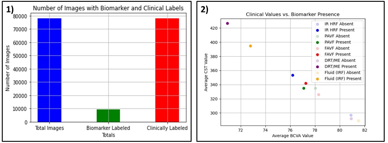
Figure 1: This gives an overview of statistics regarding biomarkers and clinical labels. 1) This shows the number of images with biomarker and clinical labels in the OLIVES dataset. 2) All 9408 OCT scans with biomarker labels were grouped based on the presence or absence of a specific biomarker. These biomarker groups were then averaged based on their associated CST and BCVA values. It can be observed that, on average, images with a biomarker present are separable from images with a biomarker absent, with respect to clinical values, thus indicating a relationship between clinical values and biomarkers.

Theoretical Interpretation

In [10] the authors present a theoretical framework for contrastive learning. Let $X$ denote the set of all possible data points. In this framework, contrastive learning assumes access to similar data in the form of $(x,x^{+})$ that comes from a distribution $D_{sim}$ as well as $k$ iid negative samples $x^{-}_{1},x^{-}_{2},...,x^{-}_{k}$ from a distribution $D_{neg}$. This idea of similarity is formalized through the introduction of a set of latent classes $C$ and an associated probability distribution $D_{c}$ over $X$ for every class $c\in C$. $D_{c}(x)$ quantifies how relevant $x$ is to class $c$ with a higher probability assigned to data points belonging to this class. Additionally, let us define $\rho$ as a distribution that describes how these classes naturally occur within the unlabeled data. From this, the positive and negative distribution are characterized as $D_{sim}=\displaystyle\mathop{\mathbb{E}}_{c\sim\rho}D_{c}(x)D_{c}(x^{+})$ and $D_{neg}=\displaystyle\mathop{\mathbb{E}}_{c\sim\rho}D_{c}(x^{-})$ where $D_{neg}$ is from the marginal of $D_{sim}$.

The key idea that separates our work from the standard contrastive learning formulation presented above is a deeper look at the relationships between $\rho$, $D_{sim}$, and $D_{neg}$. In principal, during unsupervised training, there is no information that provides the true class distribution $\rho$ of the dataset $X$. The central goal of contrastive learning is to generate an effective $D_{sim}$ and $D_{neg}$ such that the model is guided towards learning $\rho$ by identifying the distinguishing features between the two distributions. Ideally, this guidance occurs through the set of positives belonging to the same class $c_{p}$ and all negatives belonging to any class $c_{n}\neq c_{p}$ as shown in the supervised framework [11]. Traditional approaches such as [2, 12, 13], enforces positive pair similarity through augmenting a sample to define a positive pair which would clearly represent an instance belonging to the same class. However, these strategies do not define a process by which negative samples are guaranteed to belong to different classes. This problem is discussed in [10] where the authors decompose the contrastive loss $L_{un}$ as a function of an instance of a hypothesis class $f\in F$ into $L_{un}(f)=(1-\tau)L_{\neq}(f)+(\tau)L_{=}(f)$. This states that the contrastive loss is the sum of the loss suffered when the negative and positive pair come from different classes ($L_{\neq}(f)$) as well as the loss when they come from the same class ($L_{=}(f)$). In an ideal setting ($L_{=}(f)$) would approach 0, but this is impossible without direct access to the underlying class distribution $\rho$. However, it may be the case that there exists another modality of data during training that provides us with a distribution $\rho_{clin}$ with the property that the $KL(\rho_{clin}||\rho)\leq\epsilon$, where $\epsilon$ is sufficiently small. In this case, the $D_{sim}$ and $D_{neg}$ could be drawn from $\rho_{clin}$ in the form: $D_{sim}=\displaystyle\mathop{\mathbb{E}}_{c\sim\rho_{clin}}D_{c}(x)D_{c}(x^{+})$ and $D_{neg}=\displaystyle\mathop{\mathbb{E}}_{c\sim\rho_{clin}}D_{c}(x^{-})$. If $\rho_{clin}$ is a sufficiently good approximation for $\rho$, then this has a higher chance for the contrastive loss to choose positives and negatives from different class distributions and have an overall lower resultant loss. In this work, this related distribution that is in excess comes from the availability of clinical information within the unlabeled data and acts to form the $\rho_{clin}$ that we can use for choosing positives and negatives. As discussed in the introduction, this clinical data acts as a surrogate for the true distribution $\rho$ that is based on the severity of disease within the dataset and thus has the theoretical properties discussed.

Methodology

The OLIVES dataset [5] has 9408 OCT scans with explicit biomarker labels for 16 different biomarkers. The biomarker labels are organized as a 16x1 vector for each OCT scan where each entry in the vector is 1 or 0 to indicate the presence or absence of the corresponding biomarker. Of these 16 biomarkers, 5 exist in sufficiently balanced quantities to train a classifier for detection. These are Intra-Retinal Hyper-Reflective Foci (IRHRF), Partially At- tached Vitreous Face (PAVF), Fully Attached Vitreous Face (FAVF), Intra-Retinal Fluid (IRF), and Diffuse Retinal Thickening or Macular Edema (DRT/ME). This data also has 78108 OCT Scans with the clinical labels: BCVA, CST, and Eye ID. The clinical labels are discrete measurement values taken at every visit for each individual eye. These images are derived from 96 unique eyes. The dataset is split into a training set of the images from 76 eyes and the test set constitutes the images from the remaining 20 eyes. From these test OCT scans, random sampling was employed to develop an individualized test set for each of the 5 biomarkers used in our analysis. This results in a balanced test set, for each biomarker, where 500 OCT Scans have the biomarker present and 500 OCT Scans have the biomarker absent. Further details on the dataset can be found in Appendix A.1.

The overall block diagram of the proposed method is summarized in Appendix 3 Figure 5. Within the OLIVES dataset, each individual image is associated with the clinical values BCVA, CST, and Eye ID that are taken during the original patient visit. For each experiment, we first choose one of these clinical values to act as a label for each image in the dataset. A backbone network ResNet-18 [14] $f(.)$ is trained with a supervised clinical contrastive loss [11] that uses the clinical label to choose positives and negatives as shown in the first part of Figure 5. After training in this manner, the weights of the backbone network are frozen and a linear layer is appended to the output of this network. This layer is fine-tuned using the smaller subset of images containing explicit biomarker labels as shown in the second part of Figure 5. We observe in Figure 2 that a backbone trained with a clinical contrastive loss produces an embedding space that is separable with respect to individual biomarkers. Further details surrounding the training and loss function can be found in Appendix 3.

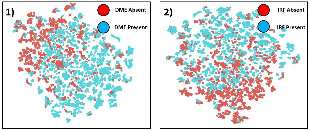
Figure 2: T-SNE visualization of the OLIVES Biomarker test set labeled by the presence or absence of DME and IRF. We can effectively achieve an embedding space that is separable with respect to biomarkers 1) DME and 2) IRF.

Results

During the clinical contrastive learning step, a single clinical label is chosen to act as the label on which positives and negatives are selected. For example, in Table 1, when CST is specified as the method, this indicates a supervised contrastive loss $L_{CST}$ where CST is utilized as the label of interest for the images in the dataset. The appended linear layer is then fine-tuned by training each biomarker individually as well as in a multi-label setting where all biomarkers are predicted simultaneously. This is reflected in Table 1 where performance in predicting each of the 5 biomarkers individually is shown by the Accuracy and F1-score for each biomarker as well as the average AUROC, Specificity , and Sensitivity to get an overall sense of performance across predicting all 5 biomarkers. We compare against 3 state of the art contrastive learning algorithms (SimCLR[2], Moco v2 [12], and PCL [13]) that are trained in the same manner with their own method for choosing positives and negatives. We observe a consistent improvement on these strategies for both individual biomarker classification performance and performance in a multi-label setting. Part of the reason for this improvement may be due to the finer granularity of tasks within the medical domain. Previous work [15] has shown that standard contrastive learning strategies are worse in situations that involve fine-grained recognition. In this case, we are attempting to detect small perturbations, rather than situations more consistent with the natural image domain where the subject of interest is present throughout the image. This acts as a preliminary explanation why the traditional strategies do comparably well for IRF and DME, but perform much worse for IRHRF, PAVF, and FAVF. IRF and DME are much easier to distinguish from the surroundng context, which is of benefit to these algorithms. This can be understood by the images in Figure 3. By leveraging a wider array of positives from the distribution of clinical labels, we observe superior performance on this biomarker detection task.

Table 1: Benchmark of the performance of supervised contrastive training on images with clinical and biomarker data. Standard deviations for the results can be found in Table 3 of Appendix B.1

Method	Biomarkers										Metrics
	IRF		DRT/ME		IRHRF		FAVF		PAVF		AUROC	Average Specificity	Average Sensitivity
	Accuracy	F1-Score	Accuracy	F1-Score	Accuracy	F1-Score	Accuracy	F1-Score	Accuracy	F1-Score
PCL [13]	76.50%	0.717	80.11%	0.761	59.10%	0.683	76.30%	0.773	51.40%	0.165	0.767	0.741	0.604
SimCLR [2]	75.13%	0.716	80.61%	0.772	59.03%	0.675	75.43%	0.761	52.69%	0.249	0.754	0.747	0.614
Moco V2 [12]	76.00%	0.720	82.24%	0.793	59.60%	0.692	75.00%	0.784	52.69%	0.211	0.770	0.762	0.651
Eye ID	72.63%	0.674	80.20%	0.778	58.00%	0.674	74.93%	0.725	65.56%	0.588	0.767	0.776	0.656
CST	75.53%	0.720	83.06%	0.811	64.30%	0.703	76.13%	0.766	62.16%	0.509	0.790	0.772	0.675
BCVA	74.03%	0.701	80.27%	0.770	58.8%	0.672	77.63%	0.785	58.06%	0.418	0.776	0.713	0.645

Conclusion

Broader Impacts

From a medical perspective, our paper shows that there are ways to utilize correlations that exist between measured clinical labels and their associated biomarker structures within images. This work potentially inspires medical research into other domains and clinical settings where questions exist as to how to effectively utilize relationships that exist within the data available. This is especially relevant in contexts where access to one modality is easier than another.

Discussion

In this work, we investigate how the usage of a supervised contrastive loss on clinical data can be used to effectively train a model for the task of biomarker classification. We show how the method performs across different combinations of clinical labels. We conclude that the usage of the clinical labels is a more effective way to leverage the correlations that exist within unlabeled data over traditional contrastive learning algorithms. We prove this through extensive experimentation on biomarkers of varying granularity within OCT scans.

Checklist

1. For all authors…

   1. Do the main claims made in the abstract and introduction accurately reflect the paper’s contributions and scope? [Yes]

   2. Did you describe the limitations of your work? [Yes] See Appendix A.2.

   3. Did you discuss any potential negative societal impacts of your work? [Yes] See Appendix A.2.

   4. Have you read the ethics review guidelines and ensured that your paper conforms to them? [Yes]

2. If you are including theoretical results…

   1. Did you state the full set of assumptions of all theoretical results? [Yes] See Theoretical Discussion Section

   2. Did you include complete proofs of all theoretical results? [N/A] Theory from paper [10] was discussed and showed connections to this paper, no explicit proof was necessary.

3. If you ran experiments…

   1. Did you include the code, data, and instructions needed to reproduce the main experimental results (either in the supplemental material or as a URL)? [Yes] See Appendix C.1

   2. Did you specify all the training details (e.g., data splits, hyperparameters, how they were chosen)? [Yes] See Appendix 3

   3. Did you report error bars (e.g., with respect to the random seed after running experiments multiple times)? [Yes] See Appendix B.1

   4. Did you include the total amount of compute and the type of resources used (e.g., type of GPUs, internal cluster, or cloud provider)? [Yes] See Appendix C.2

4. If you are using existing assets (e.g., code, data, models) or curating/releasing new assets…

   1. If your work uses existing assets, did you cite the creators? [Yes] See Appendix A.1.

   2. Did you mention the license of the assets? [Yes] See Appendix C.1.

   3. Did you include any new assets either in the supplemental material or as a URL? [N/A]

   4. Did you discuss whether and how consent was obtained from people whose data you’re using/curating? [Yes] The dataset is open source.

   5. Did you discuss whether the data you are using/curating contains personally identifiable information or offensive content? [Yes] The open source dataset discusses this point in their paper. There is no personally identifiable information within the dataset.

5. If you used crowdsourcing or conducted research with human subjects…

   1. Did you include the full text of instructions given to participants and screenshots, if applicable? [N/A]

   2. Did you describe any potential participant risks, with links to Institutional Review Board (IRB) approvals, if applicable? [N/A]

   3. Did you include the estimated hourly wage paid to participants and the total amount spent on participant compensation? [N/A]

Appendix A Dataset Description

A.1 Dataset Details

The dataset is used in this study is the OLIVES dataset [5]. Full details surrounding the dataset can be understood from the paper, but we wish to highlight specific figures from the paper to understand the studies performed in this workshop. Table 2 provides a full description of all the labels available within the dataset. It specifies the exact biomarkers and clinical labels obtained for every image as well as how they were collected. Figure 3 shows examples of the biomarkers that are detected in the studies shown in this paper. Furthermore, a complete analysis of the distributions of clinical values present in the study can be found at Figure 4.

Table 2: High-level overview of the OLIVES Dataset. The modality column details the type of data. The columns "Per Visit" and "Per Eye" indicate the amount of data in each modality on a respective visit or eye. $N_{P}$ is the number of visits that a patient $P$ takes to the clinic. The statistics across all eyes across all visits are shown in the Total Statistics column. Biomarkers are binary values, clinical labels are integers, fundus are 2D images, and OCT are 3D slices.

OLIVES Dataset Summary
Modality	Per Visit	Per Eye	Total Statistics	Overview
OCT Fundus Clinical Biomarker	49 1 4 16	$N_{P}$*49 $N_{P}$ $N_{P}$*4 1568	78189 1268 5072 150528	General: 96 Eyes, Visits every 4-16 weeks, Average 16 visits and 7 injections/patient Clinical Labels obtained every visit: BCVA, CST, Patient ID, Eye ID Biomarkers labeled: IRHRF, FAVF, IRF, DRT/ME PAVF, VD, Preretinal Tissue, EZ Disruption, IR Hemmorhages, SRF, VMT, Atrophy, SHRM, RPE Disruption, Serous PED

Figure 3: Cross-sectional images of graded biomarkers. Intra-Retinal Hyper-Reflective Foci (IRHRF), indicated by the six white arrows, are areas of hyperreflectivity in the intraretinal layers with or without shadowing of the more posterior retinal layers. Intra-Retinal Fluid (IRF) encompasses the cystic areas of hyporeflectivity. Diabetic Macular Edema (DME) is the apparent swelling and elevation of the macula due to the presence of fluid. A Partially Attached Vitreous Face (PAVF), with an arrow indicating the point of attachment and a Fully Attached Vitreous Face (FAVF). A discussion of these biomarkers can be found at [16].

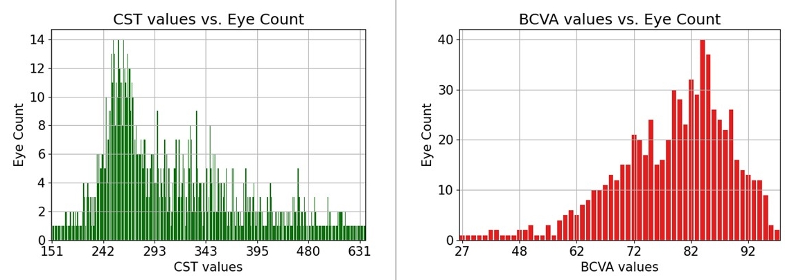
Figure 4: Distribution of CST and BCVA labels in OLIVES dataset based on number of eyes associated with each clinical value.

A.2 Limitations

The primary limitations of our study is the number of clinical labels we investigated as well as the fact the dataset comes from people who attended a single clinic. Having a wider range of clinical labels would allow us to explore how the wide range of available medical data transfers in terms of learning representations for other related tasks. Additionally, the fact the dataset comes from a single location limits how well the model can generalize towards other populations of patients. This is an inherent limitation of any medical dataset and could potentially be accounted for through supplementing analysis with other datasets such as Kermany [17] and Farisu [18]. This potential lack of generalization towards other sub-populations is problematic if not properly accounted for when applying algorithms to real-world settings. Without this accountability, this could have a negative societal impact.

Appendix B Additional Results and Training Details

B.1 Standard Deviation

The standard deviations for 3 different runs of the algorithm in the task of individual biomarker detection and average AUROC are shown in Table 3.

Method	Biomarkers
	IRF	DME	IRHRF	FAVF	PAVF	AUROC
PCL [13]	76.50% $\pm$ .513	80.11% $\pm$ .335	59.1% $\pm$ 1.03	76.30% $\pm$ .378	51.40% $\pm$ .556	.767 $\pm$ .0017
SimCLR [2]	75.13% $\pm$ .529	80.61% $\pm$ .837	59.03% $\pm$ 2.54	75.43% $\pm$ .378	52.69% $\pm$ 2.68	.754 $\pm$ .0017
Moco v2 [12]	76.00% $\pm$ .305	82.24% $\pm$ 1.38	59.6% $\pm$ .702	75.00% $\pm$ .608	52.69% $\pm$ .472	.770 $\pm$ .0035
Eye ID	72.63% $\pm$ .264	80.2% $\pm$ .384	58% $\pm$ 2.56	74.93% $\pm$ 1.36	65.56% $\pm$ .200	.767 $\pm$ .0005
CST	75.53% $\pm$ .608	83.06% $\pm$ .213	64.3% $\pm$ 2.57	76.13% $\pm$ .264	62.16% $\pm$ 1.47	.790 $\pm$ .0006
BCVA	74.03% $\pm$ .351	80.27% $\pm$ .853	58.8% $\pm$ 1.82	77.63% $\pm$ .305	58.06% $\pm$ 1.27	.776 $\pm$ .0017

Table 3: We show the performance of supervised contrastive training on the OLIVES dataset. In this table we explicitly show the standard deviation for the average across three runs for both accuracy and AUROC.

B.2 Additional Training Details

Given an input batch of data, $(x_{k}$, and clinical labels, $(y_{k}$ we obtain the set $(x_{k},y_{k})_{k=1,...,N}$. We perform augmentations on the batch twice in order to get two copies of the original batch with $2N$ images and clinical labels. These augmentations are random resize crop to a size of 224, random horizontal flips, random color jitter, and data normalization. These are sensible from a medical perspective because they don’t disrupt the general structure of the retina. This process produces a larger set $(x_{l},y_{l})_{l=1,...,2N}$ that consists of two versions of each image that differ only due to the random nature of the applied augmentation. Thus, for every image $x_{k}$ and clinical label $y_{k}$ there exists two views of the image $x_{2k}$ and $x_{2k-1}$ and two copies of the clinical labels that are equivalent to each other: $y_{2k-1}=y_{2k}=y_{k}$.

From this point, we perform the first step in Figure 5, where supervised contrastive learning is performed on the identified clinical label. The clinically labeled augmented batch is forward-propagated through an encoder network $f(\cdot)$ that we set to be the ResNet-18 architecture [14]. This results in a 512-dimensional vector $r_{i}$ that is sent through a projection network $G(\cdot)$, which further compresses the representation to a 128-dimensional embedding vector $z_{i}$. $G(\cdot)$ is chosen to be a multi-layer perceptron network with a single hidden layer. This projection network is utilized only to reduce the dimensionality of the embedding before computing the loss and is discarded after training. A supervised contrastive loss [11] is performed on the output of the projection network in order to train the encoder network. In this case, embeddings with the same clinical label are enforced to be projected closer to each other while embeddings with differing clinical labels are projected away from each other. Our introduced clinical supervised contrastive loss process can be understood by:

$$L_{supconclin}=\sum_{i\in{I}}\frac{-1}{|C(i)|}\sum_{c\in{C(i)}}log\frac{exp(z_{i}\cdot z_{c}/\tau)}{\sum_{a\in{A(i)}}exp(z_{i}\cdot z_{a}/\tau)}$$

where $i$ is the index for the image of interest $x_{i}$. All positives $c$ for image $x_{i}$ are obtained from the set $C(i)$ and all positive and negative instances $a$ are obtained from the set $A(i)$. Every element $c$ of $C(i)$ represents all other images in the batch with the same clinical label $c$ as the image of interest $x_{i}$. Additionally, $z_{i}$ is the embedding for the image of interest, $z_{c}$ represents the embedding for the clinical positives, and $z_{a}$ represents the embeddings for all positive and negative instances in the set $A(i)$. $\tau$ is a temperature scaling parameter that is set to .07 for all experiments. The loss function operates in the embedding space where the goal is to maximize the cosine similarity between embedding $z_{i}$ and its set of clinical positives $z_{c}$. It should be explicitly stated that the set $C(i)$ can represent any clinical label of interest.

After training the encoder with clinical supervised contrastive loss, we move to the second step in Figure 5 where the weights of the encoder are frozen and a linear layer is appended to the output of the encoder. This setup is trained on the available biomarker data after choosing the biomarker we wish to train for. This linear layer is trained using cross-entropy loss to distinguish between the presence or absence of the biomarker of interest in the OCT scan. In this way, we leverage knowledge learnt from training on clinical labels to improve performance on classifying biomarkers. The previously trained encoder with the supervised contrastive loss on the clinical label from step 1 produces the representation for the input and this representation is fine-tuned with the linear layer to distinguish whether or not the biomarker of interest is present.

Care was taken to ensure that all aspects of the experiments remained the same whether training was done via supervised or self-supervised contrastive learning on the encoder or cross-entropy training on the attached linear classifier. The encoder utilized was kept as a ResNet-18 architecture. The applied augmentations are random resize crop to a size of 224, random horizontal flips, random color jitter, and data normalization to the mean and standard deviation of the respective dataset. The batch size was set at 64. Training was performed for 25 epochs in every setting. A stochastic gradient descent optimizer was used with a learning rate of 1e-3 and momentum of .9.

B.3 Training of Comparison Architectures

The training for SimCLR, Moco v2, and PCL was performed using the same setup described for the supervised contrastive learning experiments described in the previous section. This means the same ResNet-18 architecture and MLP projection head was utilized. It should be noted we made appropriate changes to ResNet-18 to fit the constraints of our dataset i.e. single channel images as well as removal of an early max-pooling layer. All models were trained for 25 epochs with a batch size of 64. The applied augmentations were random resize crop to a size of 224, random horizontal flips, random color jitter, and data normalization to the mean and standard deviation of the respective dataset. A stochastic gradient descent optimizer with a learning rate of 1e-3 and momentum of .9 was used during pre-training of the backbone model as well as the appended linear layer during the biomarker classification step. Links to the code for these strategies can be found in Appendix C.1.

Additional details exist for Moco v2 and PCL in regards to certain hyperparameters introduced within their respective methodologies. For Moco v2, we used the same default hyper-parameters as introduced in the original paper. This includes a queue size of 65536, a moco momentum update term of .999, and a softmax temperature of .07. For PCL, further changes had to be made due to the clustering nature of PCL. In this case, the provided hyperparameters of PCL were based on the size of the Imagenet [19] dataset which has in excess of 1 million images. However, our training set had 60,000 images, which means that the default clustering values were inappropriate. The changes we made to fit our constraints included a queue size of 64, the number of clusters set to [100, 200, 300], the moco momentum term set to .999, and the softmax temperature scaling set to .07.

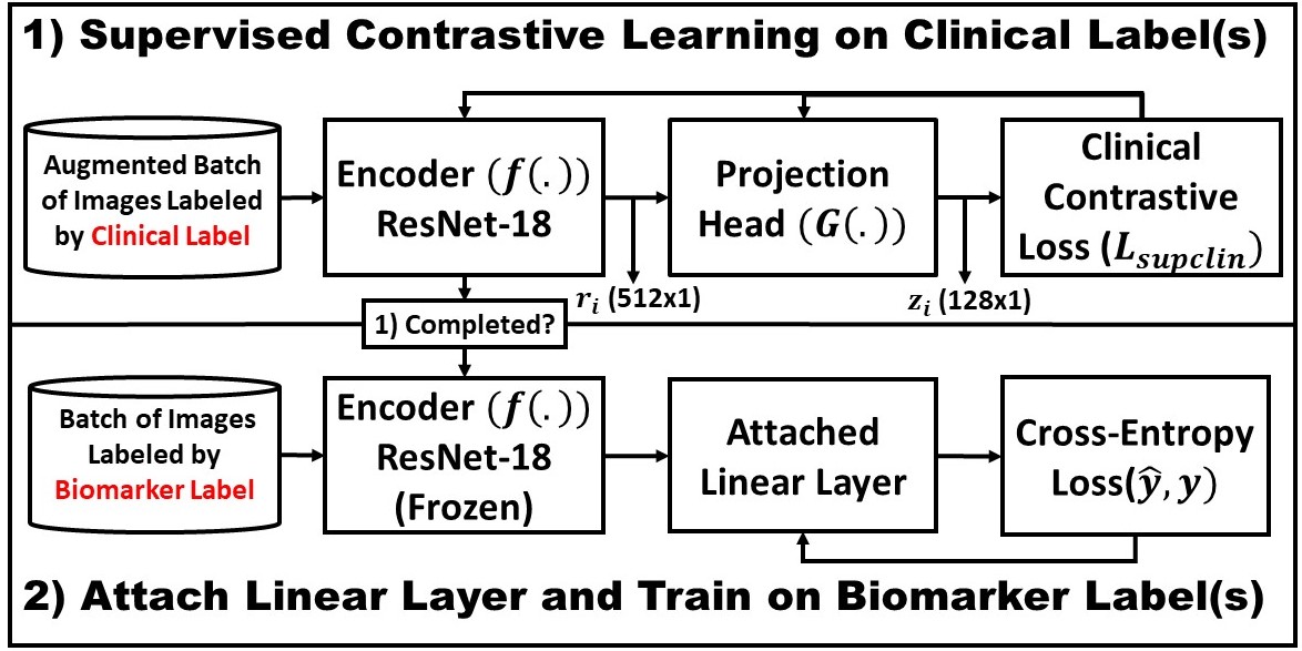
Figure 5: Overview of supervised contrastive learning and linear fine- tuning steps. 1) Supervised Contrastive Loss on clinical labels. 2) Attach linear layer and train on labeled biomarker data.

Appendix C Code and Resources

C.1 Links to Access Dataset and Code

We provide open access to the dataset. The images and labels found in the OLIVES dataset are present at:
Dataset Access
The code for the benchmarks provided in the paper are accessible at the following link:
Code Access

PCL

The code is associated with an MIT License. The DOI of the dataset is 10.5281/zenodo.6622145. The associated license with the dataset is a Creative Commons International 4 license.

The code for the comparison architectures can be found at:

SimCLR

Moco v2

C.2 Computing Resources

All experiments were run on PCs with NVIDIA GeForce GTX TITAN X 12 GB GPUs.

Appendix D Related Works

Modern contrastive learning approaches such as [2, 20, 21, 22] all generate positive pairs of images through various types of data augmentations such as random cropping, multi-cropping, and different types of blurs and color jitters. A classifier can then be trained on top of these learned representations while requiring fewer labels for satisfactory performance. Recent work has explored the idea of using medically consistent meta-data as a means of finding positive pairs of images alongside augmentations for a contrastive loss function. [23] showed that using images from the same medical pathology as well as augmentations for positive image pairs could improve representations beyond standard self-supervision. [24] demonstrated utilizing contrastive learning with a transformer can learn embeddings for electronic health records that can correlate with various disease concepts. [25] investigated choosing positive pairs from images that exist from the same patient, clinical study, and laterality. These works demonstrate the potential of utilizing clinical data within a contrastive learning framework. However, these methods were tried on limited clinical data settings, such as choosing images from the same patient or position relative to other tissues. Our work builds on these ideas by explicitly using measured clinical labels from an eye-disease setting as its own label for training a model. By doing this, we present a comprehensive assessment of what kinds of clinical data can possibly be used as a means of choosing positive instances from the perspective of OCT scans and expand the scope of how clinical data can be utilized.

References

- [1] Phuc H Le-Khac, Graham Healy, and Alan F Smeaton, “Contrastive representation learning: A framework and review,” IEEE Access, 2020.
- [2] Ting Chen, Simon Kornblith, Mohammad Norouzi, and Geoffrey Hinton, “A simple framework for contrastive learning of visual representations,” in International conference on machine learning. PMLR, 2020, pp. 1597–1607.
- [3] Kyle Strimbu and Jorge A Tavel, “What are biomarkers?,” Current Opinion in HIV and AIDS, vol. 5, no. 6, pp. 463, 2010.
- [4] Robert J McDonald, Kara M Schwartz, Laurence J Eckel, Felix E Diehn, Christopher H Hunt, Brian J Bartholmai, Bradley J Erickson, and David F Kallmes, “The effects of changes in utilization and technological advancements of cross-sectional imaging on radiologist workload,” Academic radiology, vol. 22, no. 9, pp. 1191–1198, 2015.
- [5] Mohit Prabhushankar, Kiran Kokilepersaud, Yash-yee Logan, Stephanie Trejo Corona, Ghassan AlRegib, and Charles Wykoff, “Olives dataset: Ophthalmic labels for investigating visual eye semantics,” in Proceedings of the Neural Information Processing Systems Track on Datasets and Benchmarks 2 (NeurIPS Datasets and Benchmarks 2022), 2022.
- [6] Rosana Zacarias Hannouche, Marcos Pereira de Ávila, David Leonardo Cruvinel Isaac, Alan Ricardo Rassi, et al., “Correlation between central subfield thickness, visual acuity and structural changes in diabetic macular edema,” Arquivos brasileiros de oftalmologia, vol. 75, no. 3, pp. 183–187, 2012.
- [7] Jennifer K Sun, Michael M Lin, Jan Lammer, Sonja Prager, Rutuparna Sarangi, Paolo S Silva, and Lloyd Paul Aiello, “Disorganization of the retinal inner layers as a predictor of visual acuity in eyes with center-involved diabetic macular edema,” JAMA ophthalmology, vol. 132, no. 11, pp. 1309–1316, 2014.
- [8] Tomoaki Murakami, Kazuaki Nishijima, Atsushi Sakamoto, Masafumi Ota, Takahiro Horii, and Nagahisa Yoshimura, “Association of pathomorphology, photoreceptor status, and retinal thickness with visual acuity in diabetic retinopathy,” American journal of ophthalmology, vol. 151, no. 2, pp. 310–317, 2011.
- [9] Amir H Kashani, Ingrid E Zimmer-Galler, Syed Mahmood Shah, Laurie Dustin, Diana V Do, Dean Eliott, Julia A Haller, and Quan Dong Nguyen, “Retinal thickness analysis by race, gender, and age using stratus oct,” American journal of ophthalmology, vol. 149, no. 3, pp. 496–502, 2010.
- [10] Sanjeev Arora, Hrishikesh Khandeparkar, Mikhail Khodak, Orestis Plevrakis, and Nikunj Saunshi, “A theoretical analysis of contrastive unsupervised representation learning,” arXiv preprint arXiv:1902.09229, 2019.
- [11] Prannay Khosla, Piotr Teterwak, Chen Wang, Aaron Sarna, Yonglong Tian, Phillip Isola, Aaron Maschinot, Ce Liu, and Dilip Krishnan, “Supervised contrastive learning,” arXiv preprint arXiv:2004.11362, 2020.
- [12] Xinlei Chen, Haoqi Fan, Ross Girshick, and Kaiming He, “Improved baselines with momentum contrastive learning,” arXiv preprint arXiv:2003.04297, 2020.
- [13] Junnan Li, Pan Zhou, Caiming Xiong, and Steven CH Hoi, “Prototypical contrastive learning of unsupervised representations,” arXiv preprint arXiv:2005.04966, 2020.
- [14] Kaiming He, Xiangyu Zhang, Shaoqing Ren, and Jian Sun, “Deep residual learning for image recognition,” in Proceedings of the IEEE conference on computer vision and pattern recognition, 2016, pp. 770–778.
- [15] Elijah Cole, Xuan Yang, Kimberly Wilber, Oisin Mac Aodha, and Serge Belongie, “When does contrastive visual representation learning work?,” arXiv preprint arXiv:2105.05837, 2021.
- [16] Ashish Markan, Aniruddha Agarwal, Atul Arora, Krinjeela Bazgain, Vipin Rana, and Vishali Gupta, “Novel imaging biomarkers in diabetic retinopathy and diabetic macular edema,” Therapeutic Advances in Ophthalmology, vol. 12, pp. 2515841420950513, 2020.
- [17] Daniel Kermany, Kang Zhang, Michael Goldbaum, et al., “Labeled optical coherence tomography (oct) and chest x-ray images for classification,” Mendeley data, vol. 2, no. 2, 2018.
- [18] Sina Farsiu, Stephanie J Chiu, Rachelle V O’Connell, Francisco A Folgar, Eric Yuan, Joseph A Izatt, Cynthia A Toth, Age-Related Eye Disease Study 2 Ancillary Spectral Domain Optical Coherence Tomography Study Group, et al., “Quantitative classification of eyes with and without intermediate age-related macular degeneration using optical coherence tomography,” Ophthalmology, vol. 121, no. 1, pp. 162–172, 2014.
- [19] Jia Deng, Wei Dong, Richard Socher, Li-Jia Li, Kai Li, and Li Fei-Fei, “Imagenet: A large-scale hierarchical image database,” in 2009 IEEE conference on computer vision and pattern recognition. Ieee, 2009, pp. 248–255.
- [20] Kaiming He, Haoqi Fan, Yuxin Wu, Saining Xie, and Ross Girshick, “Momentum contrast for unsupervised visual representation learning,” in Proceedings of the IEEE/CVF Conference on Computer Vision and Pattern Recognition, 2020, pp. 9729–9738.
- [21] Mathilde Caron, Ishan Misra, Julien Mairal, Priya Goyal, Piotr Bojanowski, and Armand Joulin, “Unsupervised learning of visual features by contrasting cluster assignments,” arXiv preprint arXiv:2006.09882, 2020.
- [22] Jean-Bastien Grill, Florian Strub, Florent Altché, Corentin Tallec, Pierre H Richemond, Elena Buchatskaya, Carl Doersch, Bernardo Avila Pires, Zhaohan Daniel Guo, Mohammad Gheshlaghi Azar, et al., “Bootstrap your own latent: A new approach to self-supervised learning,” arXiv preprint arXiv:2006.07733, 2020.
- [23] Shekoofeh Azizi, Basil Mustafa, Fiona Ryan, Zachary Beaver, Jan Freyberg, Jonathan Deaton, Aaron Loh, Alan Karthikesalingam, Simon Kornblith, Ting Chen, et al., “Big self-supervised models advance medical image classification,” arXiv preprint arXiv:2101.05224, 2021.
- [24] Yen-Pin Chen, Yuan-Hsun Lo, Feipei Lai, and Chien-Hua Huang, “Disease concept-embedding based on the self-supervised method for medical information extraction from electronic health records and disease retrieval: Algorithm development and validation study,” Journal of Medical Internet Research, vol. 23, no. 1, pp. e25113, 2021.
- [25] Yen Nhi Truong Vu, Richard Wang, Niranjan Balachandar, Can Liu, Andrew Y Ng, and Pranav Rajpurkar, “Medaug: Contrastive learning leveraging patient metadata improves representations for chest x-ray interpretation,” arXiv preprint arXiv:2102.10663, 2021.