From Minkowski to de Sitter Vacua with Various Geometries

Abstract

Abstract: New no-scale supergravity models with F-term SUSY breaking are introduced, adopting Kähler potentials parameterizing flat or curved (compact or non-compact) Kähler manifolds. We systematically derive the form of the superpotentials leading to Minkowski vacua. Combining two types of these superpotentials we can also determine de Sitter or anti-de Sitter vacua. The construction can be easily extended to multi-modular settings of mixed geometry. The corresponding soft SUSY-breaking parameters are also derived.

PACs numbers: 12.60.Jv, 04.65.+e

 

 

I Introduction

Within Supergravity (SUGRA) nilles ; mass , breaking Supersymmetry (SUSY) on a sufficiently flat background requires a huge amount of fine tuning, already at the classical level – see e.g. Ref. polonyi ; hall . Besides remarkable exceptions presented recently susyr , the so-called no-scale models noscale ; old ; noscale18 ; noscale19 ; Rgauged ; nsreview ; fabio ; burgess ; roest provide an elegant framework which alleviates the problem above since SUSY is broken with naturally vanishing vacuum energy along a flat direction. On the other hand, the discovery of the accelerate expansion of the present universe plcp motivates us to develop models with de Sitter (dS) – or even anti-dS (AdS) – vacua which may explain this expansion – independently of the controversy vafa ; lindev ; sevilla ; ferara surrounding this kind of (meta) stable vacua within string theory.

In two recent papers noscale18 ; noscale19 , a systematic derivation of dS/AdS vacua is presented in the context of the no-scale SUGRA without invoking any external mechanism of vacuum uplifting such as through the addition of anti-D3 brane contributions kallosh or extra Fayet-Iliopoulos terms antst . Namely, these vacua are achieved by combining two distinct Minkowski vacua taking as initial point the Kähler potential parameterizing the non-compact $SU(1,1)/U(1)$ Kähler manifold in half-plane coordinates, $T$ and $T^{*}$. Possible instabilities along the imaginary direction of the $T$ field can be cured by introducing mild deformations of the adopted geometry. The analysis has been extended to incorporate more than one superfields in conjunction with the implementation of observationally successful inflation noscaleinfl ; nsreview .

In this paper we show that the method above has a much wider applicability since it remains operational for flat spaces or curved ones. This is possible since the no-scale “character” of the models, as defined above, stems from the existence of a flat direction with SUSY broken along it, and not from the adopted moduli geometry. We parameterize the curved spaces of our models with the Poincaré disk coordinates $Z_{\alpha}$ and $Z^{*}_{\bar{\alpha}}$ which, although are widely adopted within the inflationary model building linde ; alinde ; sor , they are not frequently employed for establishing SUSY-breaking models – cf. Ref. susyr ; Rgauged . This parametrization gives us the opportunity to go beyond the non-compact geometry noscale18 ; noscale19 and establish SUSY-breaking scenaria with compact su11 or “mixed” geometry. In total, we here establish three novel uni-modular no-scale models and discuss their extensions to the multi-modular level. In all cases, we show that a subdominant quartic term noscale18 ; susyr in the Kähler potential stabilizes the sgoldstino field to a specific vacuum and provides mass for its scalar component without disturbing, though, the constant vacuum energy density. This can be identified with the present cosmological constant by finely tuning one parameter of the model whereas the others can be adjusted to perfectly natural values. If we connect, finally, our hidden sectors with some sample observable ones, non-vanishing soft SUSY-breaking (SSB) parameters soft , of the order of the gravitino mass can be readily determined at the tree level.

We start our presentation with a simplified generic argument which outlines the transition from Minkowski to dS/AdS vacua in Sec. II. We then detail our models adopting first – in Sec. III – flat moduli geometry and then – see Sec. IV – two versions of curved geometry. Generalization of our findings displaying multi-modular models with mixed geometry is presented in Sec. V. We also study in Sec. VI the communication of the SUSY breaking to the observable sector by computing the SSB terms. We summarize our results in Sec. VII. Some useful formulae related to derivation of mass spectra in SUGRA with dS/AdS vacua is arranged in Appendix A. In Appendix B we show the consistency of our results with those in Ref. noscale18 ; noscale19 translating the first ones in the language of the $T-T^{*}$ coordinates.

Unless otherwise stated, we use units where the reduced Planck scale $m_{\rm P}=2.4\cdot 10^{18}~{}{\mbox{\rm GeV}}$ is taken to be unity and the star (^∗) denotes throughout complex conjugation. Also, no summation convention is applied over the repeated Latin indices $\ell,i$ and $j$.

II Start-Up Considerations

The generation mechanism of dS/AdS vacua from a pair of Minkowski ones can be roughly established, if we consider a uni-modular model without specific geometry. In particular, we adopt a Kähler potential $K=K(Z,Z^{*})$ and attempt to determine an expression for the superpotential $W=W(Z)$ so as to construct a no-scale scenario.

The SUGRA potential $V$ based on $K$ and $W$ from Eq. (98) is written as

$$V=e^{K}\left(g_{K}^{-1}\left|\partial_{Z}W+WK_{Z}\right|^{2}-3|W|^{2}\right),$$ (1)

where $g_{K}^{-1}=K_{ZZ^{*}}^{-1}=K^{ZZ^{*}}$. Suppose that there is an expression $W=W_{0}(Z)$ which assures that the direction $Z=Z^{*}$ is classically flat with $V=0$, i.e., it provides a continuum of Minkowski vacua. The determination of $W_{0}$, based on Eq. (1), entails

$$g_{K}^{-1}\left(W_{0}^{\prime}+W_{0}K_{Z}\right)^{2}=3W_{0}^{2}~{}\Rightarrow~{}\frac{dW_{0}}{dZW_{0}}=\pm\sqrt{3g_{K}}-K_{Z}$$ (2)

with Eq. (99) being satisfied – the relevant conditions may constrain the model parameters once $K$ is specified. Here prime stands for derivation with respect to (w.r.t) $Z$. Eq. (2) admits obligatorily two solutions

$$W_{0}^{\pm}=m\exp\left(\pm\int dZ\sqrt{3g_{K}}-\int dZK_{Z}\right)$$ (3)

with $m$ a mass parameter. For the $K$’s considered below, it is easy to verify that

$$\int dZK_{Z}=K/2$$ (4)

up to a constant of integration. E.g., if $K=|Z|^{2}$, then $K_{Z}=Z$ for $Z^{*}=Z$ and $\int dZK_{Z}=Z^{2}/2=K/2$.

According to Ref. noscale18 ; noscale19 , the appearance of dS/AdS vacua is attained, if we consider the following linear combination of $W_{0}^{\pm}$ in Eq. (3)

$$W_{\Lambda}=C^{+}W_{0}^{+}-C^{-}W_{0}^{-},$$ (5)

where $C^{-}$ and $C^{+}$ are non-zero constants. As can be easily checked, $W_{\Lambda}$ does not consist solution of Eq. (2). It offers, however, the achievement of a technically natural dS/AdS vacuum since its substitution into Eq. (98) yields

$$V_{\Lambda} =e^{K}\left(g_{K}^{-1}\left(W_{\Lambda}^{\prime}+W_{\Lambda}K_{Z}\right)^{2}-3W_{\Lambda}^{2}\right)$$ (6)

$$=12e^{K}C^{-}C^{+}W_{0}^{-}W_{0}^{+}=12m^{2}C^{-}C^{+},$$

where we take into account Eqs. (3) and (4). Rigorous validation and extension (to more superfields) of this method can be accomplished via its application to specific working models. This is done in the following sections.

Let us, finally, note that $V_{\Lambda}$ can be identified with the present cosmological constant by demanding

$$V_{\Lambda}=\Omega_{\Lambda}\rho_{\rm c0}=7.2\cdot 10^{-121}m_{\rm P}^{4},$$ (7)

where $\Omega_{\Lambda}=0.6889$ and $\rho_{\rm c0}=2.4\cdot 10^{-120}h^{2}m_{\rm P}^{4}$ with $h=0.6732$ plcp is the density parameter of dark energy and the current critical energy density of the universe.

III Flat Moduli Geometry

We focus first on the models with flat internal geometry and describe below their version for one – see Sec. A – or more – see Sec. B – moduli.

A Uni-Modular Model

Our initial point is the Kähler potential

$$K_{\rm f}=|Z|^{2}-k^{2}Z_{\rm v}^{4}$$ (8)

where we include the stabilization term

$$Z_{\rm v}=Z_{+}-\sqrt{2}{\rm v}~{}~{}\mbox{with}~{}~{}Z_{\pm}=Z\pm Z^{*}.$$ (9)

Here $k$ and ${\rm v}$ are two real free parameters. Small $k$ values are completely natural, according to the ’t Hooft argument symm , since $K_{\rm f}$ enjoys an enhanced $U(1)$ symmetry which is exact for $k=0$. It is evident that the $Z$ space defined by $K_{\rm f}$ is flat with metric $\left\langle{K_{ZZ^{*}}}\right\rangle=1$ along the stable configurations

$$Z=Z^{*} ~{}~{}\mbox{for}~{}~{}k=0~{}~{}$$ (10a)

and $$\left\langle{Z}\right\rangle={\rm v}/\sqrt{2} ~{}~{}\mbox{for}~{}~{}k\neq 0.$$ (10b)

Hereafter, the value of a quantity $Q$ for both alternatives above, – i.e. either along the flat direction of Eq. (10a) or at the (stable) minimum of Eq. (10b) – is denoted by the same symbol $\left\langle{Q}\right\rangle$.

Applying Eq. (98) for $K=K_{\rm f}$, and an unknown $W=W_{\rm f}$ for $Z={Z^{*}}$, we obtain

$$V_{\rm f}=e^{Z^{2}}\left(\left(ZW_{\rm f}+W_{\rm f}^{\prime}\right)^{2}-3W_{\rm f}^{2}\right).$$ (11)

Following the strategy in Sec. II, we first find the required form of $W_{\rm f}$, $W_{0\rm f}$, which assures the establishment of a $Z$-flat direction with Minkowski vacua. I.e. we require $\left\langle{V_{\rm f}}\right\rangle=0$ for any $Z$. Solving the resulting ordinary differential equation

$$Z+\frac{dW_{0{\rm f}}}{dZW_{0\rm f}}=\pm\sqrt{3}$$ (12)

w.r.t $W_{0\rm f}$, we obtain two possible forms of $W_{0\rm f}$,

$$W_{0\rm f}^{\pm}(Z)=mwf^{\pm 1}~{}~{}\mbox{with}~{}~{}w=e^{-Z^{2}/2}~{}~{}\mbox{and}~{}~{}f=e^{\sqrt{3}Z}.$$ (13)

Note that a factor $w$ appears already in the models of Ref. noscale19 associated, though, with a matter field and not with the goldstino superfield as in our case.

The solutions in Eq. (13) above can be combined as follows – cf. Eq. (5) –

$$W_{\Lambda\rm f}=C^{+}W_{0\rm f}^{+}-C^{-}W_{0\rm f}^{-}=mwfC_{f}^{-},$$ (14)

where we introduce the symbols

$$C_{f}^{\pm}:=C^{+}\pm C^{-}f^{-2}.$$ (15)

Employing $K=K_{\rm f}$ and $W=W_{\Lambda\rm f}$ from Eqs. (8) and (14), we find the corresponding $V$ via Eq. (98)

$$V_{\rm f} =\left(m^{2}/(1-12k^{2}Z_{\rm v}^{2})\right)|f|^{2}\exp\left(-Z_{-}^{2}/2-k^{2}Z_{\rm v}^{4}\right)$$ (16)

$$\cdot\left(\left|\sqrt{3}C_{f}^{+}-Z_{-}C_{f}^{-}-4k^{2}Z_{\rm v}^{3}C_{f}^{-}\right|^{2}-3\left|C_{f}^{-}\right|^{2}\right),$$

which exhibits the dS/AdS vacua in Eqs. (10a) and (10b). Indeed, we verify that $\left\langle{V_{\rm f}}\right\rangle=V_{\Lambda}$, given in Eq. (6) and Eq. (99) for $V=V_{\rm f}$ and ${\alpha}=1$ is readily fulfilled. Indeed, decomposing $Z_{\alpha}$ (with ${\alpha}=1$ suppressed when we have just one $Z$) in real and imaginary parts, – $z_{1}:=z$ and ${\bar{z}}_{1}:={\bar{z}}$ – i.e.,

$$Z_{\alpha}=(z_{\alpha}+i{\bar{z}}_{\alpha})/\sqrt{2},$$ (17)

we find that the eigenvalues of $M_{0}^{2}$ in Eq. (100) are

$$\widehat{m}^{2}_{z\rm f}=144k^{2}m_{3/2f}^{2}\left\langle{{C_{f}^{+}}/{C_{f}^{-}}}\right\rangle^{2}~{}~{}\mbox{and}~{}~{}\widehat{m}_{{\bar{z}}\rm f}=4m_{3/2f}^{2},$$ (18)

where $m_{3/2f}$ is the $\widetilde{G}$ mass along the configurations in Eqs. (10a) and (10b). This is found by replacing $K$ and $W$ from Eqs. (8) and (14) in Eq. (103), with result

$$m_{3/2f} =m\left\langle{fC_{f}^{-}}\right\rangle$$ (19)

$$=m\begin{cases}e^{\sqrt{3}Z}\left(C^{+}-C^{-}e^{-2\sqrt{3}Z}\right)&\mbox{for}~{}~{}k=0\\ e^{\sqrt{3/2}{\rm v}}\left(C^{+}-C^{-}e^{-\sqrt{6}{\rm v}}\right)&\mbox{for}~{}~{}k\neq 0.\end{cases}$$

Note that, for $k=0$ and unfixed $Z$, $m_{3/2f}$ remains undetermined validating thereby the no-scale character of our models – cf. Ref. old ; nsreview . As a shown in Eq. (18), the real component $z$ of $Z$ remains massless due to the flatness of $V_{\rm f}$ along the direction in Eq. (10a). However, the $k$-dependent term in Eq. (8) not only stabilizes $Z$ but also provides mass to $z$. On the other hand, this term generates poles and so discontinuities in $V_{\rm f}$ – see Eq. (6). We are obliged, therefore, to focus on a local dS/AdS minimum as in Eq. (10b). Inserting Eqs. (18) and (19) into Eq. (101a) we find

$${\sf STr}M_{\rm f}^{2}=\widehat{m}^{2}_{z\rm f}+\widehat{m}^{2}_{{\bar{z}}\rm f}-4m_{3/2f}^{2}=\widehat{m}^{2}_{z\rm f},$$ (20)

which is consistent with Eq. (108) given that ${\cal R}$ in Eq. (109) is found to be $\left\langle{\mathcal{R}_{\rm f}}\right\rangle=24k^{2}$.

Fig. 1: The (dimensionless) SUGRA potential $10^{2}V_{\rm f}/m^{2}m_{\rm P}^{2}$ in Eq. (16) as a function of $z$ and ${\bar{z}}$ in Eq. (17) for the inputs shown in column A of Table 1. The location of the dS vacuum in Eq. (10b) is also depicted by a thick black point.

Our analytic findings above can be further confirmed by Fig. 1, where the dimensionless quantity $10^{2}V_{\rm f}/m^{2}m_{\rm P}^{2}$ is plotted as a function of $z$ and ${\bar{z}}$ in Eq. (17). We employ the values of the parameters listed in column A of Table 1 – obviously $k_{1}$ there is identified with $k$ in Eq. (8). We see that the dS vacuum in Eq. (10b) – indicated by the black thick point – is placed at $(z,{\bar{z}})=(1,0)$ and is stabilized w.r.t both directions. In the same column of Table 1 displayed are also the various masses of $\widetilde{G}$ and the scalar ($\widehat{z}$) and pseudoscalar ($\widehat{\bar{z}}$) components of the sgoldstino $Z$ given in GeV for convenience. For $N=1$, the spectrum does not comprise any goldstino $(\widehat{\tilde{z}})$ as explained in Appendix A. It is worth mentioning that the aforementioned masses may acquire quite natural values (of the order of $10^{-15}$) for logical values of the relevant parameters despite the fact that the fulfilment of Eq. (7) via Eq. (6) requires a tiny $C^{-}$. E.g., for the parameters given in Table 1 we need $C^{-}=1.4\cdot 10^{-90}$.

Let us, finally, note that performing a Kähler transformation

$$K\rightarrow K+\Lambda_{K}+\Lambda_{K}^{*}\>\>\>\mbox{and}\>\>\>W\rightarrow We^{-\Lambda_{K}},$$ (21)

with $K=K_{\rm f}$ and $W=W_{\Lambda\rm f}$ in Eqs. (8) and (14) respectively and $\Lambda_{K}=-Z^{2}/2$, the present model is equivalent with that described by the following $K$ and $W$

$$\widetilde{K}_{\rm f}=-\frac{1}{2}Z_{-}^{2}-k^{2}Z_{\rm v}^{4}~{}~{}\mbox{and}~{}~{}\widetilde{W}_{\Lambda\rm f}=mfC_{f}^{-}.$$ (22)

From the form above we can easily infer that, for $k\rightarrow 0$, $\widetilde{K}_{\rm f}$ enjoys the enhanced symmetries

$$Z\rightarrow Z+c~{}~{}\mbox{and}~{}~{}Z\rightarrow-Z,$$ (23)

where $c$ is a real number. These are more structured than the simple $U(1)$ mentioned below Eq. (8) and underline, once more, the naturality of the possible small $k$ values. In this limit, a similar model arises in the context of the ${\alpha}$-scale SUGRA introduced in Ref. roest .

Table 1: A Case Study Overview

Case:	A	B	C	D	E	F
Input Settings
$K$	$K_{\rm f}$	$K_{2\rm f}$	$K_{\boldsymbol{+}}$	$K_{\boldsymbol{-}}$	$K_{\boldsymbol{+}-}$	$K_{\rm f\boldsymbol{-}}$
$W$	$W_{\Lambda\rm f}$	$W_{\Lambda 2\rm f}$	$W_{\Lambda\boldsymbol{+}}$	$W_{\Lambda\boldsymbol{-}}$	$W_{\Lambda\boldsymbol{+}-}$	$W_{\Lambda\rm f\boldsymbol{-}}$
Input Parameters
${\rm v}_{\alpha}=m_{\rm P}$, $C^{+}=0.01$ and $m=5~{}{\mbox{\rm TeV}}$
$k_{1}$	$0.3$	$0.3$	$0.3$	$0.3$	$0.3$	$0.3$
$k_{2}$	$-$	$0.2$	$-$	$-$	$0.2$	$0.2$
$a_{1}$	$-$	$1$	$-$	$-$	$1$	$1$
$n_{1}$	$-$	$-$	$1$	$4$	$1$	$4$
$n_{2}$	$-$	$-$	$-$	$-$	$4$	$-$
Particle Masses in GeV
$\widetilde{G}$	$170$	$276$	$145$	$180$	$263$	$288$
$\widehat{z}_{1}$	$612$	$572$	$960$	$530$	$744$	$599$
$\widehat{{\bar{z}}}_{1}$	$340$	$551$	$581$	$180$	$1005$	$577$
$\widehat{z}_{2}$	$-$	$540$	$-$	$-$	$422$	$528$
$\widehat{{\bar{z}}}_{2}$	$-$	$551$	$-$	$-$	$372$	$466$
$\widehat{\tilde{z}}_{1}$	$-$	$276$	$-$	$-$	$263$	$288$

B Multi-Modular Model

The model above can be extended to incorporate more than one modulus. In this case, the corresponding $K$ is written as

$$K_{N\rm f}=\sum_{\ell=1}^{N_{\rm f}}\left(|Z_{\ell}|^{2}-k_{\ell}^{2}Z_{{\rm v}\ell}^{4}\right)$$ (24)

where for any modulus $Z_{{\alpha}}$ we include a stabilization term

$$Z_{\rm v{\alpha}}=Z_{{\alpha}+}-\sqrt{2}{\rm v}_{\alpha}~{}~{}\mbox{with}~{}~{}Z_{{\alpha}\pm}=Z_{\alpha}\pm Z^{*}_{\alpha},$$ (25)

with ${\alpha}=\ell$ in the domain of the values shown in Eq. (24). As we verify below, for the same ${\alpha}$ values, we can obtain the stable configurations

$$Z_{{\alpha}-}=0 ~{}~{}\mbox{for}~{}~{}k_{\alpha}=0$$ (26a)

and $$\left\langle{Z_{\alpha}}\right\rangle={\rm v}_{\alpha}/\sqrt{2} ~{}~{}\mbox{for}~{}~{}k_{\alpha}\neq 0.$$ (26b)

Along them the Kähler metric is represented by a $N_{\rm f}\times N_{\rm f}$ diagonal matrix

$$\left\langle{K_{{\alpha}{\bar{\beta}}}}\right\rangle={\sf diag}(1,...,1).$$ (27)

Setting $Z_{\ell}=Z_{\ell}^{*}$, $K=K_{N\rm f}$ from Eq. (24) and $W=W_{N\rm f}(Z_{\ell})$ in Eq. (98), $V$ takes the form

$$V_{N\rm f}=e^{\sum_{\ell}Z_{\ell}^{2}}\left(\mbox{$\sum_{\ell}$}\left(Z_{\ell}W_{N\rm f}+\partial_{\ell}W_{N\rm f}\right)^{2}-3W_{N\rm f}^{2}\right).$$ (28)

Setting $V_{N\rm f}=0$ and assuming the following form for the corresponding $W_{N\rm f}$

$$W_{0N\rm f}(Z_{1},...,Z_{N_{\rm f}}) = \prod_{\ell}W_{{\rm f}\ell}(Z_{\ell})\Rightarrow$$

$$\partial_{\ell}W_{0N\rm f} = {dW_{{\rm f}\ell}\over dZ_{\ell}}{W_{0N\rm f}\over W_{{\rm f}\ell}},$$ (29)

we obtain the separated differential equations

$$\sum_{\ell}\left(Z_{\ell}+\frac{dW_{{\rm f}\ell}}{dZ_{\ell}W_{{\rm f}\ell}}\right)^{2}=3.$$ (30)

These can be solved w.r.t $W_{{\rm f}\ell}$, if we set

$$Z_{\ell}+\frac{dW_{{\rm f}\ell}}{dZ_{\ell}W_{{\rm f}\ell}}=|a_{\ell}|~{}~{}\mbox{with}~{}~{}\sum_{\ell}a_{\ell}^{2}=3,$$ (31)

i.e., the $a_{\ell}$’s satisfy the equation of the hypersphere $\mathbb{S}^{N_{\rm f}-1}$ with radius $\sqrt{3}$. The resulting solutions take the form

$$W_{{\rm f}\ell}^{\pm}=w_{\ell}f_{\ell}^{\pm{a_{\ell}}/{\sqrt{3}}}~{}~{}\mbox{with}~{}~{}w_{\ell}=e^{-Z_{\ell}^{2}/2}~{}~{}\mbox{and}~{}~{}f_{\ell}=e^{\sqrt{3}Z_{\ell}}.$$ (32)

The total expression for $W_{0N\rm f}$ is found substituting the findings above into Eq. (29). Namely,

$$W_{0N\rm f}^{\pm}=m\prod_{\ell}W_{{\rm f}\ell}^{\pm}=m{\cal W}F^{\pm 1},$$ (33)

where we define the functions

$${\cal W}=e^{-\sum_{\ell}Z_{\ell}^{2}/2}~{}~{}\mbox{and}~{}~{}F=e^{\sum_{\ell}a_{\ell}Z_{\ell}}.$$ (34)

As in the case with $N_{\rm f}=1$, we combine both solutions above as follows

$$W_{\Lambda N\rm f}=C^{+}W_{0N\rm f}^{+}-C^{-}W_{0N\rm f}^{-}=m{\cal W}FC_{F}^{-},$$ (35)

where we introduce the “generalized” $C$ symbols – cf. Eq. (15)

$$C_{F}^{\pm}:=C^{+}\pm C^{-}F^{-2}.$$ (36)

Substituting Eqs. (24) and (35) into Eq. (98) we find that $V$ takes the form

$$V_{N\rm f} =m^{2}|F|^{2}\exp\left(-\sum_{\ell}\left(Z_{\ell-}^{2}/2+k_{\ell}^{2}Z_{{\rm v}\ell}^{4}\right)\right)$$ (37)

$$\cdot\left(\sum_{\ell}\frac{\left|a_{\ell}C_{F}^{+}-Z_{\ell-}C_{F}^{-}-4k_{\ell}^{2}Z_{{\rm v}\ell}^{3}C_{F}^{-}\right|^{2}}{1-12k_{\ell}^{2}Z_{{\rm v}\ell}^{2}}-3\left|C_{F}^{-}\right|^{2}\right).$$

We can confirm that $V_{N\rm f}$ admits the dS/AdS vacua in Eqs. (26a) and (26b) for ${\alpha}=\ell$, since $\left\langle{V_{N\rm f}}\right\rangle=V_{\Lambda}$, given in Eq. (6). In addition, Eq. (99) for $V=V_{N\rm f}$ and ${\alpha}=\ell$ is satisfied, since the $2N_{\rm f}$ masses squared of the relevant matrix in Eq. (100) are positive. Indeed, analyzing $Z_{\ell}$ in real and imaginary parts as in Eq. (17), we find

$$\widehat{m}_{z\rm f\ell}^{2} = 48k_{\ell}^{2}a_{\ell}^{2}m_{3/2F}^{2}\left\langle{{C_{F}^{+}}/{C_{F}^{-}}}\right\rangle^{2};$$ (38a)

$$\widehat{m}_{\bar{z}\rm f\ell}^{2} = 4m_{3/2F}^{2}\left(1+(3-a_{\ell}^{2})V_{\Lambda}/6{m_{3/2F}^{2}}\right),$$ (38b)

where $m_{3/2}$ for the present case is computed inserting Eqs. (24) and (35) into Eq. (103) with result

$$\hskip 56.9055ptm_{3/2F}=m\left\langle{FC_{F}^{-}}\right\rangle=$$ (39)

$$m\cdot\begin{cases}e^{\sum_{\ell}a_{\ell}Z_{\ell}}\left(C^{+}-C^{-}e^{-2\sum_{\ell}a_{\ell}Z_{\ell}}\right)&\mbox{for}~{}~{}k_{\ell}=0\\ e^{\sum_{\ell}a_{\ell}\frac{{\rm v}_{\ell}}{\sqrt{2}}}\left(C^{+}-C^{-}e^{-\sqrt{2}\sum_{\ell}a_{\ell}{\rm v}_{\ell}}\right)&\mbox{for}~{}~{}k_{\ell}\neq 0.\end{cases}$$

The expressions above conserve the basic features of the no-scale models as explained below Eq. (19). We consider the stabilized version of these models (with $k_{\alpha}\neq 0$) as more complete since it offers the determination of $m_{3/2}$ and avoids the presence of a massless mode which may be problematic.

We should note that the relevant $2N_{\rm f}\times 2N_{\rm f}$ matrix $M_{0}^{2}$ of Eq. (100) turns out to be diagonal up to some tiny mixings appearing in the ${\bar{z}}_{\ell}-{\bar{z}}_{\bar{\ell}}$ positions. These contributions though can be safely neglected since these are proportional to $V_{\Lambda}$. We also obtain $N_{\rm f}-1$ Weyl fermions with masses $\widehat{m}_{\tilde{z}\tilde{\ell}}=m_{3/2}$ where $\tilde{\ell}=1,...,N_{\rm f}-1$. Note that Eqs. (39), (38a) and (38b) reduce to the ones obtained for $N_{\rm f}=1$, i.e. Eqs. (19) and (18), if we replace $a_{\ell}=\sqrt{3}$. Inserting the mass spectrum above into Eq. (101a), we find

$${\sf STr}M_{N\rm f}^{2}=2(N_{\rm f}-1)\left(m_{3/2F}^{2}+V_{\Lambda}\right)+\mbox{$\sum_{\ell}$}\widehat{m}^{2}_{z\rm f\ell}.$$ (40)

This result is consistent with Eq. (101b) given that its last term turns out to be equal to the last term of Eq. (40).

To highlight further the conclusions above we depict in Fig. 2 the dimensionless $V_{N\rm f}$ for $N=2$, i.e. $V_{2\rm f}$, as a function of $z_{1}$ and $z_{2}$ for ${\bar{z}}_{1}={\bar{z}}_{2}=0$ and the other parameters displayed in column B of Table 1. We observe that the dS vacuum in Eq. (26b) – indicated by a black thick point in the plot – is well stabilized against both directions. In the same column of Table 1 we also arrange some suggestive values of the particle masses for $N=2$. Note that, due to the smallness of $V_{\Lambda}$, the $\widehat{m}_{{\bar{z}}\rm f\ell}$ values are practically equal between each other.

Fig. 2: The (dimensionless) SUGRA potential $V_{2\rm f}/m^{2}m_{\rm P}^{2}$ in Eq. (37) as a function of $z_{1}$ and $z_{2}$ in Eq. (17) for ${\bar{z}}_{1}={\bar{z}}_{2}=0$ and the inputs shown in column B of Table 1. The location of the dS vacuum in Eq. (26b) is also depicted by a thick black point.

IV Curved Moduli Geometry

We proceed now to the models with curved internal geometry and describe below their version for one – see Sec. A – or more – see Sec. B – moduli.

A Uni-Modular Model

The curved moduli geometry is described mainly by the Kähler potentials

$$K_{\boldsymbol{\pm}}=\pm n\ln\Omega_{\boldsymbol{\pm}}~{}~{}\mbox{with}~{}~{}\Omega_{\boldsymbol{\pm}}=1\pm\frac{|Z|^{2}-k^{2}Z_{\rm v}^{4}}{n}$$ (41)

and $Z_{\rm v}$ given in Eq. (9). Also $n>0$ and $k$ are real, free parameters. The positivity of the argument of logarithm in Eq. (41) implies

$$1\pm|Z|^{2}/n\gtrsim 0~{}~{}\Rightarrow\begin{cases}|Z|^{2}\gtrsim-n&\mbox{for}~{}~{}K=K_{\boldsymbol{+}},\\ |Z|\lesssim\sqrt{n}&\mbox{for}~{}~{}K=K_{\boldsymbol{-}}.\end{cases}$$ (42)

The restriction for $K=K_{\boldsymbol{+}}$ is trivially satisfied, whereas this for $K=K_{\boldsymbol{-}}$ defines the allowed domain of $Z$ values which lie in a disc with radius $\sqrt{n}$ and thus, the name disk coordinates. If we set $k=0$ in Eq. (41), $K_{\boldsymbol{-}}$ parameterizes noscale ; su11 ; nsreview the coset space $SU(1,1)/U(1)$ whereas $K_{\boldsymbol{+}}$ is associated su11 with $SU(2)/U(1)$. Thanks to these symmetries, low $k$ values are totally natural as we explained below Eq. (23). The Kähler metric and (the constant) $\mathcal{R}$ in Eq. (109) are respectively

$$K_{ZZ^{*}}=\Omega_{\boldsymbol{\pm}}^{-2}~{}~{}\mbox{and}~{}~{}\mathcal{R}_{\rm\pm}=\pm 2/n~{}~{}\mbox{for}~{}~{}K=K_{\boldsymbol{\pm}}.$$ (43)

The last quantity reveals that the Kähler manifold is compact (spherical) or non-compact (hyperbolic) if $K=K_{\boldsymbol{+}}$ or $K=K_{\boldsymbol{-}}$ respectively. For this reason, the bold subscripts ${\boldsymbol{+}}$ or ${\boldsymbol{-}}$ associated with various quantities below are referred to $K=K_{\boldsymbol{+}}$ or $K=K_{\boldsymbol{-}}$ respectively.

Repeating the procedure described in Sec. II, we find the form of $V$ in Eq. (98), $V_{\boldsymbol{\pm}}$, as a function of $K=K_{\boldsymbol{\pm}}$ in Eq. (41) and $W=W_{\boldsymbol{\pm}}$ for $Z={Z^{*}}$. This is

$$V_{\boldsymbol{\pm}}=v_{\boldsymbol{\pm}}^{\pm n}W_{\boldsymbol{\pm}}^{2}\left(\left(Z+v_{\boldsymbol{\pm}}\frac{W_{\boldsymbol{\pm}}^{\prime}}{W_{\boldsymbol{\pm}}}\right)^{2}-3\right)~{}\mbox{with}~{}~{}v_{\boldsymbol{\pm}}=1\pm\frac{Z^{2}}{n}.$$ (44)

Setting $V_{\boldsymbol{\pm}}=0$ we see that the corresponding $W_{\boldsymbol{\pm}}=W_{0\boldsymbol{\pm}}$ obeys the differential equation

$$\frac{dW_{0\boldsymbol{\pm}}}{W_{0\boldsymbol{\pm}}}=\frac{\pm\sqrt{3}-Z}{v_{\boldsymbol{\pm}}}dZ.$$ (45)

This can be resolved yielding two possible forms of $W_{0\boldsymbol{\pm}}$,

$$W_{0\boldsymbol{\pm}}^{\pm}=m{v}^{\mp n/2}_{\boldsymbol{\pm}}u_{\boldsymbol{\pm}}^{\pm 1}~{}~{}\mbox{for}~{}~{}K=K_{\boldsymbol{\pm}},$$ (46)

which assure the establishment of Minkowski minima – cf. Eq. (3). The corresponding functions $u_{\boldsymbol{\pm}}$ can be specified as follows

$$u_{\boldsymbol{+}}=e^{\sqrt{3n}{\rm atn}(Z/n)}~{}~{}\mbox{and}~{}~{}u_{\boldsymbol{-}}=e^{\sqrt{3n}{\rm atnh}(Z/n)},$$ (47)

where ${\rm atn}$ and ${\rm atnh}$ stand for the functions $\arctan$ and ${\rm arctanh}$ respectively. The superscript $\pm$ in Eq. (46) correspond to the exponents of $u_{\boldsymbol{\pm}}$ and should not be confused with the bold subscripts ${\boldsymbol{\pm}}$ with reference to $K_{\boldsymbol{\pm}}$.

Combining both Minkowski solutions, $W_{0\boldsymbol{\pm}}^{\pm}$ in Eq. (46) and introducing the shorthand notation – cf. Eq. (15) –

$$C_{u\boldsymbol{\pm}}^{\pm}:=C^{+}\pm C^{-}u_{\boldsymbol{\pm}}^{-2}~{}~{}\mbox{for}~{}~{}K=K_{\boldsymbol{\pm}},$$ (48)

we can obtain the superpotential

$$W_{\Lambda\boldsymbol{\pm}} =C^{+}W_{0\boldsymbol{\pm}}^{+}-C^{-}W_{0\boldsymbol{\pm}}^{-}$$ (49)

$$=mv_{\boldsymbol{\pm}}^{\mp n/2}u_{\boldsymbol{\pm}}C_{u\boldsymbol{\pm}}^{-}~{}~{}\mbox{for}~{}~{}K=K_{\boldsymbol{\pm}}$$

which allows for dS/AdS vacua. To verify it, we insert $K=K_{\boldsymbol{\pm}}$ and $W=W_{\rm\Lambda\boldsymbol{\pm}}$ from Eqs. (41) and (49) in Eq. (98) with result

$$V_{\boldsymbol{\pm}} =m^{2}\Omega_{\boldsymbol{\pm}}^{\pm n}|v_{\boldsymbol{\pm}}|^{\mp n}|u_{\boldsymbol{\pm}}|^{2}\Big{(}-3|C_{u\boldsymbol{\pm}}^{-}|^{2}+n\Omega_{\boldsymbol{\pm}}^{2}$$ (50)

$$\cdot\left|(\sqrt{3}C_{u\boldsymbol{\pm}}^{+}-ZC_{u\boldsymbol{\pm}}^{-})v_{\boldsymbol{\pm}}^{-1}\pm(Z^{*}-4k^{2}Z_{\rm v}^{3})C_{u\boldsymbol{\pm}}^{-}\Omega_{\boldsymbol{\pm}}^{-1}\right|^{2}$$

$$\cdot\left(\mp|4k^{2}Z_{\rm v}^{3}-Z|^{2}+n\Omega_{\boldsymbol{\pm}}(1-12k^{2}Z_{\rm v}^{2})\right)^{-1}\Big{)}.$$

Given that for $Z_{-}=0$ we get $\Omega_{\boldsymbol{\pm}}=v_{\boldsymbol{\pm}}$, we may infer that $\left\langle{V_{\boldsymbol{\pm}}}\right\rangle=V_{\Lambda}$ shown in Eq. (6) for the directions in Eqs. (10a) and (10b). Eq. (99) for $V=V_{\boldsymbol{\pm}}$ and $Z_{1}:=Z$ is also valid without restrictions for $K=K_{\boldsymbol{+}}$ but only for $n>3$ for $K=K_{\boldsymbol{-}}$. In fact, employing the decomposition of $Z$ in Eq. (17) for ${\alpha}=1$, we can obtain the scalar spectrum of our models which includes the sgoldstino components with masses squared

$$\widehat{m}_{z\boldsymbol{\pm}}^{2} = 144k^{2}m_{3/2\boldsymbol{\pm}}^{2}\left\langle{v_{\boldsymbol{\pm}}^{3/2}\left|{C_{u\boldsymbol{\pm}}^{+}}/{C_{u\boldsymbol{\pm}}^{-}}\right|}\right\rangle^{2};$$ (51a)

$$\widehat{m}_{{\bar{z}}\boldsymbol{\pm}}^{2} = 4m_{3/2\boldsymbol{\pm}}^{2}\left(1\pm(3/n)\left\langle{C_{u\boldsymbol{\pm}}^{+}/C_{u\boldsymbol{\pm}}^{-}}\right\rangle^{2}\right)$$ (51b)

for $K=K_{\boldsymbol{\pm}}$ respectively. The corresponding $m_{3/2}$ according to Eq. (103) – with $K$ and $W$ given in Eqs. (41) and (49) – is

$$m_{3/2\boldsymbol{\pm}}=m\left\langle{u_{\boldsymbol{\pm}}C_{u\boldsymbol{\pm}}^{-}}\right\rangle~{}~{}\mbox{for}~{}~{}K=K_{\boldsymbol{\pm}},$$ (52)

which may be explicitly written if we use Eqs. (47) and (48) – cf. Eq. (19). The stability of configurations in Eqs. (10a) and (10b) is protected for $\widehat{m}_{{\bar{z}}\boldsymbol{-}}^{2}>0$ and $\widehat{m}_{{\bar{z}}\boldsymbol{-}}^{2}>0$ provided that

$$Z<\sqrt{n}~{}~{}\mbox{and}~{}~{}n>3~{}~{}\mbox{for}~{}~{}K=K_{\boldsymbol{-}}.$$ (53)

Since we expect that $Z\leq 1$, the latter restriction is capable to circumvent both requirements – see column D in Table 1. Inserting the mass spectrum above into the definition of Eq. (101a), we can find

$${\sf STr}M_{\boldsymbol{\pm}}^{2}=12m_{3/2\boldsymbol{\pm}}^{2}\left\langle{C_{u\boldsymbol{\pm}}^{+}/C_{u\boldsymbol{\pm}}^{-}}\right\rangle^{2}\left(12nk^{2}\left\langle{v_{\boldsymbol{\pm}}}\right\rangle^{3}\pm 1\right).$$ (54)

It can be easily verified that the result above is consistent with the expression of Eq. (108) given that $\mathcal{R}$ in Eq. (109) is

$$\left\langle{\mathcal{R}_{\boldsymbol{\pm}}}\right\rangle=2\left(12k^{2}n\left\langle{v_{\boldsymbol{\pm}}}\right\rangle^{3}\pm 1\right).$$ (55)

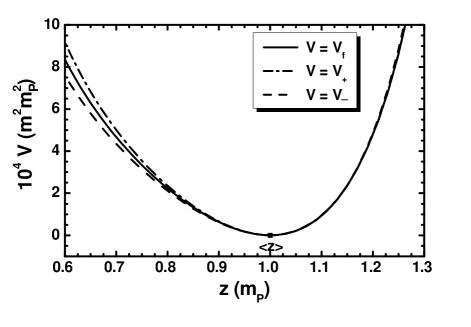
Fig. 3: The (dimensionless) SUGRA potential $V/m^{2}m_{\rm P}^{2}$ as a function of $z$ for ${\bar{z}}=0$ and the settings in columns A (solid line), C (dot-dashed line) and D (dashed line) of Table 1. The value $\left\langle{z}\right\rangle=m_{\rm P}$ is also indicated.

Our analytic results are exemplified in Fig. 3, where we depict $V_{\boldsymbol{+}}$ (dot-dashed line) $V_{\boldsymbol{-}}$ (dashed line) together with $V_{\rm f}$ (solid line) versus $z$ for ${\bar{z}}=0$, $k=k_{1}=0.3$ and the other parameters shown in columns A, C and D of Table 1. Note that the selected $n=n_{1}=4$ for $K=K_{\boldsymbol{-}}$ protects the stability of the vacuum in Eq. (10b) as dictated above. In columns C and D of Table 1 we display some explicit values of the particle masses encountered for $K=K_{\boldsymbol{-}}$ and $K_{\boldsymbol{+}}$ respectively. As a consequence of the employed $n$ value in column D we accidentally obtain $m_{3/2\boldsymbol{-}}=\widehat{m}_{{\bar{z}}1}=\widehat{m}_{{\bar{z}}-}$; ${k_{1}}$ and $n_{1}$ obviously coincide with $k$ and $n$ in Eq. (41).

B Multi-Modular Model

The generalization of the model above to incorporate more than one modulus can be performed following the steps of Sec. B. This generalization, however, is accompanied by a possible mixing of the two types of the curved geometry analyzed in Sec. A. More specifically, the considered here $K$, includes two sectors with $N_{\boldsymbol{+}}$ compact components and $N_{\boldsymbol{-}}$ non-compact ones. It may be written as

$$K_{N_{\boldsymbol{+}}N_{\boldsymbol{-}}}=\sum_{i=1}^{N_{\boldsymbol{+}}}n_{i}\ln\Omega_{i}+\sum_{j=N_{\boldsymbol{+}}+1}^{N_{\boldsymbol{\pm}}}n_{j}\ln\Omega_{j},$$ (56)

where $N_{\boldsymbol{\pm}}=N_{\boldsymbol{+}}+N_{\boldsymbol{-}}$ and the arguments of the logarithms are identified as

$$\Omega_{\alpha}=\begin{cases}\Omega_{{\alpha}\boldsymbol{+}}&~{}~{}\mbox{for}~{}~{}{\alpha}=i,\\ \Omega_{{\alpha}\boldsymbol{-}}&~{}~{}\mbox{for}~{}~{}{\alpha}=j.\end{cases}$$ (57a)

The symbols $$\Omega_{{\alpha}\boldsymbol{\pm}}$$ can be collectively defined as

$$\Omega_{{\alpha}\boldsymbol{\pm}}=1\pm|Z_{\alpha}|^{2}/n_{\alpha}\mp k_{\alpha}^{2}Z_{\rm v{\alpha}}^{4}$$ (57b)

with $Z_{{\rm v}{\alpha}}$ is given from Eq. (25) and ${\alpha}=i,j$. When explicitly indicated, summation and multiplication over $i$ and $j$ is applied for the range of their values specified in Eq. (56). Given that $i$ corresponds to compact geometry (${\boldsymbol{+}}$) and $j$ to non-compact (${\boldsymbol{-}}$) we remove the relevant indices ${\boldsymbol{\pm}}$ from the various quantities to simplify the notation. Under these assumptions, the positivity of the arguments of $\ln$ implies restrictions only to $\Omega_{j}$ – cf. Eq. (42):

$$\Omega_{j}>0~{}~{}\Rightarrow~{}~{}|Z_{j}|<\sqrt{n_{j}}\,.$$ (58)

Along the configurations in Eqs. (26a) and (26b) for ${\alpha}=i,j$, the Kähler metric is represented by a $N_{\boldsymbol{\pm}}\times N_{\boldsymbol{\pm}}$ diagonal matrix

$$K_{{\alpha}{\bar{\beta}}}={\sf diag}(v_{1}^{-2},...,v_{N_{+}}^{-2},v_{N_{+}+1}^{-2},...,v_{N_{\boldsymbol{\pm}}}^{-2}),$$ (59)

where we introduce the generalizations of the symbols $v_{\boldsymbol{\pm}}$, defined in Eq. (44), as follows

$$v_{i}=(1+Z_{i}^{2}/n_{i})~{}~{}\mbox{and}~{}~{}v_{j}=(1-Z_{j}^{2}/n_{j}).$$ (60)

Also $\mathcal{R}$ in Eq. (109) includes contributions for both geometric sectors, i.e,

$$\mathcal{R}_{N_{\boldsymbol{+}}N_{\boldsymbol{-}}}=2\mbox{$\sum_{i}$}n_{i}^{-1}-2\mbox{$\sum_{j}$}n_{j}^{-1}.$$ (61)

Inserting $K=K_{N_{\boldsymbol{+}}N_{\boldsymbol{-}}}$ from Eq. (56) and $W=W_{N\boldsymbol{\pm}}(Z_{i},Z_{j})$ with $Z_{i}=Z^{*}_{i}$ and $Z_{j}=Z^{*}_{j}$ in Eq. (98), we obtain

$$V_{N\boldsymbol{\pm}} = \mathcal{V}^{-2}\Big{(}\mbox{$\sum_{i}$}\left(Z_{i}W_{N\boldsymbol{\pm}}+\partial_{i}W_{N\boldsymbol{\pm}}v_{i}\right)^{2}$$ (62)

$$+ \mbox{$\sum_{j}$}\left(Z_{j}W_{N\boldsymbol{\pm}}+\partial_{j}W_{N\boldsymbol{\pm}}v_{j}\right)^{2}-3W_{N\boldsymbol{\pm}}^{2}\Big{)},$$

where the prefactor $\mathcal{V}$ is defined as follows

$$\mathcal{V}=\mbox{$\prod_{i,j}$}v_{i}^{-n_{i}/2}v_{j}^{n_{j}/2}.$$ (63)

Setting $V_{N\boldsymbol{\pm}}=0$ and assuming the ansatz for the corresponding $W_{N\boldsymbol{\pm}}$

$$W_{0N\boldsymbol{\pm}}(Z_{1},...,Z_{N_{\boldsymbol{\pm}}})=\prod_{i,j}W_{i}(Z_{i})W_{j}(Z_{j})~{}~{}\Rightarrow~{}~{}$$

$$\frac{\partial_{i}W_{0N\boldsymbol{\pm}}}{W_{0N\boldsymbol{\pm}}}={dW_{i}\over dZ_{i}W_{i}}~{}~{}\mbox{and}~{}~{}\frac{\partial_{j}W_{0N\boldsymbol{\pm}}}{W_{0N\boldsymbol{\pm}}}={dW_{j}\over dZ_{j}W_{j}},$$ (64)

we obtain the separated differential equations

$$\sum_{i}\left(Z_{i}+\frac{dW_{i}}{dZ_{i}W_{i}}v_{i}\right)^{2}+\sum_{j}\left(Z_{j}+\frac{dW_{j}}{dZ_{j}W_{j}}v_{j}\right)^{2}=3.$$ (65)

We can solve the equations above if we set

$$Z_{i}+\frac{dW_{i}}{dZ_{i}W_{i}}v_{i}=|a_{i}|~{}~{}\mbox{and}~{}~{}Z_{j}+\frac{dW_{j}}{dZ_{j}W_{j}}v_{j}=|a_{j}|$$ (66)

imposing the constraint

$$\mbox{$\sum_{i}$}a_{i}^{2}+\mbox{$\sum_{j}$}a_{j}^{2}=3,$$ (67)

i.e., the $a_{i}$ and $a_{j}$ can be regarded as coordinates of the hypersphere $\mathbb{S}^{N_{\boldsymbol{\pm}}-1}$ with radius $\sqrt{3}$. Solution of the differential equations above w.r.t $W_{i}$ and $W_{j}$ yields

$$W_{i}^{\pm}=v_{i}^{-n_{i}/2}u_{i}^{\pm a_{i}/\sqrt{3}}~{}~{}\mbox{and}~{}~{}W_{j}^{\pm}=v_{j}^{n_{i}/2}u_{j}^{\pm a_{j}/\sqrt{3}}$$ (68)

with the generalizations of $u_{\boldsymbol{+}}$ and $u_{\boldsymbol{-}}$ in Eq. (47) defined as

$$u_{i}=e^{\sqrt{3n_{i}}{\rm atn}(Z_{i}/\sqrt{n_{i}})}\\ ~{}~{}\mbox{and}~{}~{}u_{j}=e^{\sqrt{3n_{j}}{\rm atnh}(Z_{j}/\sqrt{n_{j}})}.$$ (69)

Upon substitution of Eq. (68) into Eq. (64) we obtain

$$W_{0N\boldsymbol{\pm}}^{\pm}=m\prod_{i,j}W_{i}^{\pm}W_{j}^{\pm}=m\mathcal{V}\mathcal{U}^{\pm 1},$$ (70)

where we define the function

$$\mathcal{U}=\mbox{$\prod_{i,j}$}u_{i}^{a_{i}/\sqrt{3}}u_{j}^{a_{j}/\sqrt{3}}.$$ (71)

Introducing the generalized $C$ symbols – cf. Eq. (15) –

$$C_{\mathcal{U}}^{\pm}:=C^{+}\pm C^{-}\mathcal{U}^{-2},$$ (72)

we combine both solutions in Eq. (70) as follows

$$W_{\Lambda N\boldsymbol{\pm}}=C^{+}W_{0N\boldsymbol{\pm}}^{+}-C^{-}W_{0N\boldsymbol{\pm}}^{-}=m\mathcal{V}\mathcal{U}C_{\mathcal{U}}^{-}.$$ (73)

Plugging $K=K_{N_{\boldsymbol{+}}N_{\boldsymbol{-}}}$ and $W=W_{\Lambda N\boldsymbol{\pm}}$ from Eqs. (56) and (73) in Eq. (98) we find

$$V_{N\boldsymbol{\pm}} =m^{2}\left(\mbox{$\prod_{ij}$}\Omega_{i}^{n_{i}}\Omega_{j}^{-n_{j}}\right)|\mathcal{V}\mathcal{U}|^{2}\Bigg{(}-3|C_{\mathcal{U}}^{-}|^{2}$$ (74)

$$+\sum_{i}\Big{(}n_{i}\Omega_{i}^{2}\cdot\left|(a_{i}C_{\mathcal{U}}^{+}-Z_{i}C_{\mathcal{U}}^{-})v_{i}^{-1}\right.$$

$$+\left.(Z^{*}_{i}-4k_{i}^{2}Z_{{\rm v}i}^{3})C_{\mathcal{U}}^{-}\Omega_{i}^{-1}\right|^{2}$$

$$\cdot\left(-\left|4k_{i}^{2}Z_{{\rm v}i}^{3}-Z_{i}\right|^{2}+n_{i}\Omega_{i}\left(1-12k_{i}^{2}Z_{{\rm v}i}^{2}\right)\right)^{-1}\Big{)}$$

$$+\sum_{j}\Big{(}n_{j}\Omega_{j}^{2}\cdot\left|(a_{j}C_{\mathcal{U}}^{+}-Z_{j}C_{\mathcal{U}}^{-})v_{j}^{-1}\right.$$

$$-\left.(Z^{*}_{j}-4k_{j}^{2}Z_{{\rm v}j}^{3})C_{\mathcal{U}}^{-}\Omega_{j}^{-1}\right|^{2}$$

$$\cdot\left(\left|4k_{j}^{2}Z_{{\rm v}j}^{3}-Z_{j}\right|^{2}+n_{j}\Omega_{j}\left(1-12k_{j}^{2}Z_{{\rm v}j}^{2}\right)\right)^{-1}\Big{)}\Bigg{)}.$$

Note that there are slight differences between the terms with subscripts $i$ and $j$ due to our convention in Eq. (57a) – cf. Eq. (50). The settings in Eqs. (26a) and (26b) consist honest dS/AdS vacua since $\left\langle{V_{N\boldsymbol{\pm}}}\right\rangle=V_{\Lambda}$ given in Eq. (6). However, the conditions in Eq. (99) for $V=V_{N\boldsymbol{\pm}}$ and ${\alpha}=i,j$ are met only after imposing upper bound on ${\rm v}_{j}$ and $a_{j}$. To determine this, we extract the masses squared of the $2N_{\boldsymbol{\pm}}$ scalar components of $Z_{i}$ and $Z_{j}$ in Eq. (17) which are

$$\widehat{m}_{zi\boldsymbol{+}}^{2} = 48k_{i}^{2}a_{i}^{2}m_{3/2{\cal U}}^{2}\left\langle{v_{i}^{3/2}{C_{\mathcal{U}}^{+}}/{C_{\mathcal{U}}^{-}}}\right\rangle^{2};$$ (75a)

$$\widehat{m}_{zj\boldsymbol{-}}^{2} = 48k_{j}^{2}a_{j}^{2}m_{3/2{\cal U}}^{2}\left\langle{v_{j}^{3/2}{C_{\mathcal{U}}^{+}}/{C_{\mathcal{U}}^{-}}}\right\rangle^{2};$$ (75b)

$$\widehat{m}_{{\bar{z}}i\boldsymbol{+}}^{2} \simeq 4m_{3/2{\cal U}}^{2}\left(1+a_{i}^{2}/n_{i}\right);$$ (75c)

$$\widehat{m}_{{\bar{z}}j\boldsymbol{-}}^{2} \simeq 4m_{3/2{\cal U}}^{2}\left(1-a_{j}^{2}/n_{j}\right),$$ (75d)

where we restore the $\boldsymbol{\pm}$ symbols for clarity and we neglect for simplicity terms of order $(C^{-})^{2}$ in the two last expressions. We also compute $m_{3/2}$ upon substitution of Eqs. (56) and (73) into Eq. (103) with result

$$m_{3/2{\cal U}}=m\left\langle{\mathcal{U}C_{\mathcal{U}}^{-}}\right\rangle.$$ (76)

As in the case of Sec. B, the relevant matrix $M_{0}^{2}$ in Eq. (100) turns out to be essentially diagonal since the non-zero elements appearing in the ${\bar{z}}_{\alpha}-{\bar{z}}_{\beta}$ positions with ${\alpha},\beta=i,j$ are proportional to $V_{\Lambda}$ and can be safely ignored compared to the diagonal terms. From Eqs. (75b) and (75d), we notice that positivity of $\widehat{m}_{zj-}^{2}$ and $\widehat{m}_{{\bar{z}}j-}^{2}$ dictates

$$Z_{j}<\sqrt{n_{j}}~{}~{}\mbox{and}~{}~{}|a_{j}|<\sqrt{n_{j}}.$$ (77)

These restrictions together with Eq. (67) delineate the allowed ranges of parameters in the hyperbolic sector. We also obtain $N_{\boldsymbol{\pm}}-1$ Weyl fermions with masses $\widehat{m}_{\tilde{z}\tilde{\alpha}}=m_{3/2}$ with $\tilde{\alpha}=1,...,N_{\boldsymbol{\pm}}-1$. Inserting the mass spectrum above into Eq. (101a) we find

$${\sf STr}M_{N\boldsymbol{\pm}}^{2} \simeq 6m_{3/2{\cal U}}^{2}\Bigg{(}(N_{\boldsymbol{\pm}}-1)+\frac{2}{3}\left(\mbox{$\sum_{i}$}\frac{a_{i}^{2}}{n_{i}}+\mbox{$\sum_{j}$}\frac{a_{j}^{2}}{n_{j}}\right)+$$ (78)

$$8\left\langle{\frac{C_{\mathcal{U}}^{+}}{C_{\mathcal{U}}^{-}}}\right\rangle^{2}\left(\mbox{$\sum_{i}$}a_{i}^{2}k_{i}^{2}\left\langle{v_{i}}\right\rangle^{3}+\mbox{$\sum_{j}$}a_{j}^{2}k_{j}^{2}\left\langle{v_{j}}\right\rangle^{3}\right)\Bigg{)}.$$

It can be checked that this result is consistent with Eq. (101b).

Fig. 4: The (dimensionless) SUGRA potential $V_{\boldsymbol{+}-}/m^{2}m_{\rm P}^{2}$ in Eq. (74) as a function of $z_{1}$ and $z_{2}$ in Eq. (17) for ${\bar{z}}_{1}={\bar{z}}_{2}=0$ and the inputs shown in column E of Table 1. The location of the dS vacuum in Eq. (26b) is also depicted by a thick black point.

For $N=2$, $N_{\boldsymbol{-}}=N_{\boldsymbol{+}}=1$ and the parameters shown in column E of Table 1, we present in Fig. 4 the relevant $V_{N\boldsymbol{\pm}}$, $V_{2\boldsymbol{\pm}}=V_{\boldsymbol{+}-}$ – conveniently normalized – versus $z_{1}$ and $z_{2}$ in Eq. (17) fixing ${\bar{z}}_{1}={\bar{z}}_{2}=0$. It is clearly shown that the vacuum of Eq. (26b), depicted by a bold point, is indeed stable. In column E of Table 1 we arrange also some representative masses (in GeV) of the particle spectrum for $N_{\boldsymbol{\pm}}=2$. From the parameters listed there we infer that $a_{2}=\sqrt{2}<\sqrt{n_{2}}=2$ and so Eqs. (67) and (77) are met.

V Generalization

It is certainly impressive that the models described in Sec. B and B can be combined in a simple and (therefore) elegant way. We here just specify the utilized $K$ and $W$ of a such model and restrict ourselves to the verification of the results. In particular, we consider the following $K$

$$K_{N\rm f\boldsymbol{\pm}}=K_{N\rm f}+K_{N_{\boldsymbol{+}}N_{\boldsymbol{-}}},$$ (79)

which incorporates the individual contributions from Eqs. (24) and (56). It is intuitively expected that the required $W$ for achieving dS/AdS vacua has the form – cf. Eqs. (35) and (73)

$$W_{\Lambda N\rm f\boldsymbol{\pm}}=C^{+}W_{0N\rm f\boldsymbol{\pm}}^{+}+C^{-}W_{0N\rm f\boldsymbol{\pm}}^{-},$$ (80)

where the definitions of $W_{0N\rm f\boldsymbol{\pm}}^{\pm}$ follow those in Eqs. (33) and (70) respectively. Namely, we set

$$W_{0N\rm f\boldsymbol{\pm}}^{\pm}=m\mathcal{W}\mathcal{V}(F\mathcal{U})^{\pm 1},$$ (81)

where the parameters $a_{\ell},a_{i}$ and $a_{j}$, which enter the expressions of the functions $F$ and $\mathcal{U}$ in Eqs. (34) and (71), satisfy the constraint – cf. Eqs. (31) and (67)

$$\mbox{$\sum_{\ell}$}a_{\ell}^{2}+\mbox{$\sum_{i}$}a_{i}^{2}+\mbox{$\sum_{j}$}a_{j}^{2}=3.$$ (82)

I.e., they lie at the hypersphere $\mathbb{S}^{N_{\rm t}-1}$ with radius $\sqrt{3}$ and $N_{\rm t}=N_{\rm f}+N_{\boldsymbol{\pm}}$. If we introduce, in addition, the $C$ symbols – cf. Eqs. (36) and (72) –

$$C_{F\mathcal{U}}^{\pm}:=C^{+}\pm C^{-}(F\mathcal{U})^{-2},$$ (83)

$W_{\Lambda N\rm f\boldsymbol{\pm}}$ in Eq. (80) is simplified as

$$W_{\Lambda N\rm f\boldsymbol{\pm}}=m\mathcal{W}\mathcal{V}F\mathcal{U}C_{F\mathcal{U}}^{-}.$$ (84)

Plugging $K=K_{N\rm f\boldsymbol{\pm}}$ and $W=W_{\Lambda N\rm f\boldsymbol{\pm}}$ from Eqs. (79) and (84) into Eq. (98) we obtain

$$V_{N\rm f\boldsymbol{\pm}} = m^{2}e^{K_{N\rm f}}\left(\mbox{$\prod_{ij}$}\Omega_{i}^{n_{i}}\Omega_{j}^{-n_{j}}\right)|F\mathcal{V}\mathcal{U}|^{2}\Bigg{(}-3|C_{F\mathcal{U}}^{-}|^{2}$$ (85)

$$+ \sum_{i}\Big{(}n_{i}\Omega_{i}^{2}\cdot\left|(a_{i}C_{F\mathcal{U}}^{+}-Z_{i}C_{F\mathcal{U}}^{-})v_{i}^{-1}\right.$$

$$+ \left.(Z^{*}_{i}-4k_{i}^{2}Z_{{\rm v}i}^{3})C_{F\mathcal{U}}^{-}\Omega_{i}^{-1}\right|^{2}$$

$$\cdot \left(-\left|4k_{i}^{2}Z_{{\rm v}i}^{3}-Z_{i}\right|^{2}+n_{i}\Omega_{i}\left(1-12k_{i}^{2}Z_{{\rm v}i}^{2}\right)\right)^{-1}\Big{)}$$

$$+ \sum_{j}\Big{(}n_{j}\Omega_{j}^{2}\cdot\left|(a_{j}C_{F\mathcal{U}}^{+}-Z_{j}C_{F\mathcal{U}}^{-})v_{j}^{-1}\right.$$

$$- \left.(Z^{*}_{j}-4k_{j}^{2}Z_{{\rm v}j}^{3})C_{F\mathcal{U}}^{-}\Omega_{j}^{-1}\right|^{2}$$

$$\cdot \left(\left|4k_{j}^{2}Z_{{\rm v}j}^{3}-Z_{j}\right|^{2}+n_{j}\Omega_{j}\left(1-12k_{j}^{2}Z_{{\rm v}j}^{2}\right)\right)^{-1}\Big{)}$$

$$+ \sum_{\ell}\left|a_{\ell}C_{F\mathcal{U}}^{+}-Z_{\ell-}C_{F\mathcal{U}}^{-}-4k_{\ell}^{2}Z_{{\rm v}\ell}^{3}C_{F\mathcal{U}}^{-}\right|^{2}$$

$$\cdot \left(1-12k_{\ell}^{2}Z_{{\rm v}\ell}^{2}\right)^{-1}\Bigg{)}.$$

Once again, we infer that Eqs. (26a) and (26b) consist dS/AdS vacua since $\left\langle{V_{N\rm f\boldsymbol{\pm}}}\right\rangle=V_{\Lambda}$ – see Eq. (6) – and Eq. (99) with $V=V_{N\rm f\boldsymbol{\pm}}$ and ${\alpha}=\ell,i,j$ is fulfilled if we take into account the restrictions in Eqs. (77) and (58).

The $\widetilde{G}$ mass is derived from Eq. (103), after substituting $K$ and $W$ from Eqs. (79) and (84) respectively. The result is

$$m_{3/2{\cal FU}}=m\left\langle{F\mathcal{U}C_{F\mathcal{U}}^{-}}\right\rangle.$$ (86)

From Eqs. (100) and (105) with ${\alpha}=\ell,i,j$, we can obtain the mass spectrum of the present model which includes $2N_{\rm t}$ real scalars and $N_{\rm t}-1$ Weyl fermions with masses $\widehat{m}_{\tilde{z}{\alpha}}=m_{3/2}$ where ${\alpha}=1,...,N_{\rm t}-1$. The masses squared of the $2N_{\rm f}$ scalars are given in the $C^{-}\rightarrow 0$ limit by Eqs. (38a) and (38b) for $C_{F}^{+}/C_{F}^{-}=1$ and $m_{3/2F}$ replaced by $m_{3/2{\cal FU}}$. In the same limit the masses squared of the $2N_{\boldsymbol{\pm}}$ scalars are given by Eq. (75a) – (75d) for $C_{\mathcal{U}}^{+}/C_{\mathcal{U}}^{-}=1$ and $m_{3/2{\cal U}}$ replaced by $m_{3/2{\cal FU}}$.

To provide a pictorial verification of our present setting, we demonstrate in Fig. 5 the three-dimensional plot of $V_{N\rm f\boldsymbol{\pm}}$ with $N_{\rm f}=N_{\boldsymbol{-}}=1$ and $N_{\boldsymbol{+}}=0$, i.e. $V_{1\rm f\boldsymbol{-}}$, versus $z_{1}$ and $z_{2}$ for ${\bar{z}}_{1}={\bar{z}}_{2}=0$ – see Eq. (17) – and the other parameters arranged in column F of Table 1. Note that the subscripts $1$ and $2$ of $z$ correspond to $\ell=1$ and $j=1$ and the validity of Eqs. (77) and (82) is protected. It is evident that the ground state, depicted by a tick black point is totally stable. Some characteristic values of the masses of the relevant particles are also arranged in column F of Table 1.

Fig. 5: The (dimensionless) SUGRA potential $V_{\rm f\boldsymbol{-}}/m^{2}m_{\rm P}^{2}$ in Eq. (85) as a function of $z_{1}$ and $z_{2}$ for ${\bar{z}}_{1}={\bar{z}}_{2}=0$ – see Eq. (17) – and the inputs shown in column F of Table 1. The location of the dS vacuum in Eq. (26b) is also depicted by a thick black point.

VI Link to the Observable Sector

Our next task is to study the transmission of the SUSY breaking to the visible world. Here we restrict for simplicity ourselves to the cases with just one Goldstino superfield, $Z$. To implement our analysis, we introduce the chiral superfields of the observable sector $\Phi_{\alpha}$ with ${\alpha}=1,...,5$ and assume the following structure – cf. Ref. nilles ; susyr ; soft – for the total superpotential, $W_{\rm HO}$, of the theory

$$W_{\rm HO}=W_{\rm H}(Z)+W_{\rm O}\left(\Phi_{\alpha}\right),$$ (87)

where $W_{\rm H}$ is given by Eq. (14) or Eq. (49) for flat or curved $Z$ geometry respectively whereas $W_{\rm O}$ has the following generic form

$$W_{\rm O}=h\Phi_{1}\Phi_{2}\Phi_{3}+\mu\Phi_{4}\Phi_{5}.$$ (88)

with $h$ and $\mu$ free parameters. On the other hand, we consider three variants of the total $K$ of the theory, $K_{\rm HO}$, ensuring universal SSB parameters for $\Phi_{\alpha}$:

$$K_{1\rm HO} =K_{\rm H}(Z)+\mbox{$\sum_{\alpha}$}|\Phi_{\alpha}|^{2};~{}~{}~{}$$ (89a)

$$K_{2\rm HO} =K_{\rm H}(Z)+N_{\rm O}\ln\left(1+\mbox{$\sum_{\alpha}$}|\Phi_{\alpha}|^{2}/N_{\rm O}\right),$$ (89b)

where $$K_{\rm H}(Z) K_{\rm f} K_{\pm} Z N_{\rm O} Z$$ may be identified with in Eq. (8) or in Eq. (41) for flat or curved geometry respectively whereas may remain unspecified. For curved geometry we may introduce one more variant

$$K_{3\rm HO}=\pm n\ln\Big{(}\Omega_{\boldsymbol{\pm}}\pm\mbox{$\sum_{\alpha}$}|\Phi_{\alpha}|^{2}/n\Big{)}.$$ (89c)

If we expand the $K_{\rm HO}$’s above for low $\Phi_{\alpha}$ values, these may assume the form

$$K_{\rm HO}=K_{\rm H}(Z)+\widetilde{K}_{\rm H}(Z)|\Phi_{\alpha}|^{2},$$ (90a)

with $$\widetilde{K}_{\rm H}$$ being identified as

$$\widetilde{K}_{\rm H}=\begin{cases}1&\mbox{for}~{}~{}K_{\rm HO}=K_{1\rm HO},K_{2\rm HO};\\ \Omega_{\boldsymbol{\pm}}^{-1}&\mbox{for}~{}~{}K_{\rm HO}=K_{3\rm HO}\,.\end{cases}$$ (90b)

Adapting the general formulae of Ref. soft ; susyr to the case with one hidden-sector field and tiny $\left\langle{V}\right\rangle$, we obtain the SSB terms in the effective low energy potential which can be written as

$$V_{\rm SSB}=m_{\alpha}^{2}|\widehat{}\Phi_{\alpha}|^{2}+\left(A\widehat{h}\widehat{}\Phi_{1}\widehat{}\Phi_{2}\widehat{}\Phi_{3}+B\widehat{\mu}\widehat{}\Phi_{4}\widehat{}\Phi_{5}+{\rm h.c.}\right),$$ (91)

where the rescaled parameters are

$$\widehat{h}=e^{\langle{K_{\rm H}}\rangle/2}\langle{\widetilde{K}_{\rm H}}\rangle^{-3/2}h~{}~{}\mbox{and}~{}~{}\widehat{\mu}=e^{\langle{K_{\rm H}}\rangle/2}\langle{\widetilde{K}_{\rm H}}\rangle^{-1}\mu$$ (92)

and the canonically normalized fields are $\widehat{}\Phi_{\alpha}=\langle{\widetilde{K}_{\rm H}}\rangle^{1/2}\Phi_{\alpha}$.

In deriving the values of the SSB parameters above, we distinguish the cases:

(a)

For flat $Z$ geometry, i.e. $K_{\rm H}=K_{\rm f}$, we see from Eq. (90b) that $\widetilde{K}_{\rm H}$ is constant for both adopted $K_{\rm HO}$’s and so, the results are common. Substituting

$$\left\langle{F^{Z}}\right\rangle=\sqrt{3}m_{3/2f}~{}~{}\mbox{and}~{}~{}\left\langle{\partial_{Z}K_{\rm H}}\right\rangle={\rm v},$$ (93)

into the relevant expressions susyr we arrive at

$$m_{\alpha} =\left(1+e^{\sqrt{6}{\rm v}}{V_{\Lambda}}/{m^{2}\left\langle{C_{f}^{-}}\right\rangle^{2}}\right)m_{3/2f}\simeq m_{3/2f},$$ (94)

$$A =-\sqrt{\frac{3}{2}}{\rm v}\left\langle{\frac{C_{f}^{+}}{C_{f}^{-}}}\right\rangle m_{3/2f}\simeq\sqrt{\frac{3}{2}}{\rm v}m_{3/2f},$$

$$B =A-m_{3/2f},$$

where $(\widehat{h},\widehat{\mu})=e^{{\rm v}^{2}/4}(h,\mu)$ and the last simplified expressions are obtained in the realistic limit $C^{-}\rightarrow 0$ which implies $C_{f}^{+}/C_{f}^{-}\rightarrow-1$.

(b)

For curved $Z$ geometry, i.e. $K_{\rm H}=K_{\boldsymbol{\pm}}$, we can distinguish two subcases depending on which $K_{\rm HO}$ from those shown in Eq. (89a) – (89c) is selected. Namely,

• If $K_{\rm HO}=K_{1\rm HO}$ or $K_{2\rm HO}$, then $\widetilde{K}_{\rm H}$ in Eq. (90b) is $Z$ independent. For $K_{\rm H}=K_{\boldsymbol{\pm}}$ respectively we find

  $$(m_{\alpha},A,B)=\left(1,\sqrt{3/2}{\rm v},A/m_{3/2\boldsymbol{\pm}}-1\right)m_{3/2\boldsymbol{\pm}},$$ (95)

  where $(\widehat{h},\widehat{\mu})=\left\langle{v_{\boldsymbol{\pm}}}\right\rangle^{\pm n/2}(h,\mu)$ and we take into account the following

  $$\left\langle{F^{Z}}\right\rangle=\sqrt{3}\left\langle{v_{\boldsymbol{\pm}}}\right\rangle m_{3/2\boldsymbol{\pm}}~{}~{}\mbox{and}~{}~{}~{}\left\langle{\partial_{Z}K_{\boldsymbol{\pm}}}\right\rangle=\left\langle{Zv_{\boldsymbol{\pm}}^{-1}}\right\rangle.$$

• If $K_{\rm HO}=K_{3\rm HO}$, then $\widetilde{K}_{\rm H}$ in Eq. (90b) is $Z$ dependent. Inserting the expressions

  $$\left\langle{\partial_{Z}\ln\widetilde{K}_{\rm H}}\right\rangle=\frac{1}{n\left\langle{v_{\boldsymbol{\pm}}}\right\rangle^{2}}~{}~{}\mbox{and}\left\langle{\partial_{Z}\ln\widetilde{K}_{\rm H}^{2}}\right\rangle=\frac{2{\rm v}}{n\left\langle{v_{\boldsymbol{\pm}}}\right\rangle}$$

  into the general formulae soft ; susyr we end up with the following results for $K_{\rm H}=K_{\boldsymbol{\pm}}$ correspondingly:

  $$m_{\alpha} =\sqrt{1\pm 3/n}\,m_{3/2\boldsymbol{\pm}};$$ (96)

  $$A =\sqrt{3/2}{\rm v}(1\pm 3/n)m_{3/2\boldsymbol{\pm}};$$

  $$B =\left(\sqrt{3/2}{\rm v}(1\pm 2/n)-1\right)m_{3/2\boldsymbol{\pm}},$$

  where $\widehat{h}=\left\langle{v_{\boldsymbol{\pm}}}\right\rangle^{(3\pm n)/2}h$ and $\widehat{\mu}=\left\langle{v_{\boldsymbol{\pm}}}\right\rangle^{(2\pm n)/2}\mu$.

In both cases above we take $C^{-}\simeq 0$ for simplicity. Note that the condition $n>3$ for $K=K_{\boldsymbol{-}}$ which is imperative for the stability of the configurations in Eqs. (10a) and (10b) – see Eq. (51b) – implies non-vanishing SSB parameters too. Taking advantage from the numerical inputs listed in columns A, C and D of Table 1 (for the three unimodular models) we can obtain some explicit values for the SSB parameters derived above – restoring units for convenience. Our outputs are arranged in the three rightmost columns of Table 2 for the specific forms of $W_{\rm H},K_{\rm H}$ and $K_{\rm HO}$ in Eqs. (87) and (90a) shown in the three leftmost columns. We remark that there is a variation of the achieved values of SSB parameters which remain of the order of the $\widetilde{G}$ mass in all cases.

Table 2: SSB Parameters: a Case Study for the Inputs of Table 1.

Input Settings			SSB Parameters in GeV
$W_{\rm H}$	$K_{\rm H}$	$\widetilde{K}_{\rm H}$	$m_{\alpha}$	$|A|$	$|B|$
$W_{\Lambda\rm f}$	$K_{\rm f}$	$1$	$170$	$208$	$378$
$W_{\Lambda\boldsymbol{+}}$	$K_{\rm\boldsymbol{+}}$	$1$	$145$	$177$	$32$
$W_{\Lambda\boldsymbol{+}}$	$K_{\rm\boldsymbol{+}}$	$1/\Omega_{\boldsymbol{+}}$	$290$	$711$	$388$
$W_{\Lambda\boldsymbol{-}}$	$K_{\rm\boldsymbol{-}}$	$1$	$179$	$220$	$40$
$W_{\Lambda\boldsymbol{-}}$	$K_{\rm\boldsymbol{-}}$	$1/\Omega_{\boldsymbol{-}}$	$90$	$55$	$69$

VII Conclusions

We have extended the approach of Ref. noscale18 ; noscale19 , proposing new no-scale SUGRA models which lead to Minkowski, dS and AdS vacua without need for any external uplifting mechanism. We first provided a simple but general enough argument which assists to appreciate the effectiveness of our paradigm. We then adopted specific single-field models and showed that the achievement of dS/AdS solutions using pairs of Minkowski ones works perfectly well for flat – see Eqs. (8) and (14) – and hyperbolic or spherical geometry – see Eqs. (41) and (49). We also broadened these constructions to multi-field models – see Sec. B, B and V. Within each case we derived the SUGRA potential and the relevant mass spectrum paying special attention to the stability of the proposed solutions. Typical representatives of our results were illustrated in Fig. 1 – 5 employing numerical inputs from Table 1. We provided, finally, the set of the soft SUSY-breaking parameters induced by our unimodular models linking them to a generic observable sector – see Eqs.  (94) - (96). We verified – see Table 2 – that their magnitude is of the order of the gravitino mass.

As stressed in Ref. noscale19 ; noscaleinfl , this kind of constructions, based exclusively in SUGRA, can be considered as part of an effective theory valid below $m_{\rm P}$. However, the correspondence between Kähler and super-potentials which yields naturally Minkowski, dS and AdS (locally stable) vacua with broken SUSY may be a very helpful guide for string theory so as to establish new possible models with viable low energy phenomenology. As regards the ultraviolet completion, it would be interesting to investigate if our models belong to the string landscape or swampland vafa . Note that the swampland string conjectures are generically not satisfied in SUGRA-based models but there are suggestions ferara ; sevilla which may work in our framework too. One more open issue is the interface of our settings with inflation. We aspire to return on this topic soon taking advantage from other similar studies noscaleinfl ; ketov ; lhclinde ; ant – see Ref. deinf . At last but not least, let us mention that the achievement of the present value of the dark-energy density parameter in Eq. (7) requires an inelegant fine tuning, which may be somehow alleviated if we take into account contributions from the electroweak symmetry breaking and/or the confinement in quantum chromodynamics noscale19 ; noscaleinfl .

Despite the shortcomings above, we believe that the establishment of novel models for SUSY breaking with a natural emergence of Minkowski and dS/AdS vacua can be considered as an important development which offers the opportunity for further explorations towards several cosmo-phenomenological directions.

Acknowledgment

This research work was supported by the Hellenic Foundation for Research and Innovation (H.F.R.I.) under the “First Call for H.F.R.I. Research Projects to support Faculty members and Researchers and the procurement of high-cost research equipment grant” (Project Number: 2251).

Dedication

I would like to dedicate the present paper to the memory of T. Tomaras, an excellent University teacher who let his imprint on my first post-graduate steps.

Appendix A Mass Formulae In SUGRA

We here generalize our formulae in Ref. susyr for $N$ chiral multiplets and dS/AdS vacua. Let us initially remind that central role in the SUGRA formalism plays the Kähler-invariant function expressed in terms of the Kähler potential $K$ and the superpotential $W$ as follows

$$G:=K+\ln|W|^{2}.$$ (97)

Using it we can derive the F-term scalar potential nilles

$$V=e^{G}\left(G^{{\alpha}{\bar{\beta}}}G_{\alpha}G_{\bar{\beta}}-3\right)=e^{K}|W|^{2}\left(K^{{\alpha}{\bar{\beta}}}G_{\alpha}G_{\bar{\beta}}-3\right),$$ (98)

where the subscripts of quantities $G$ and $K$ denote differentiation w.r.t the superfields $Z_{\alpha}$ and $G^{{\alpha}{\bar{\beta}}}=K^{{\alpha}{\bar{\beta}}}$ is the inverse of the Kähler  metric $K_{{\alpha}{\bar{\beta}}}$. The spontaneous SUSY breaking takes place typically at a (locally stable) vacuum or flat direction of $V$ which satisfies the extremum and minimum conditions

$$\left\langle{\partial_{{\alpha}}V}\right\rangle=\left\langle{\partial_{\bar{\alpha}}V}\right\rangle=0~{}~{}\mbox{and}~{}~{}\widehat{m}_{A}^{2}>0.$$ (99)

Here $\partial_{{\alpha}}:=\partial/\partial Z_{\alpha}$ and $\partial_{\bar{\alpha}}:=\partial/\partial Z^{*}_{\bar{\alpha}}$ with the scalar components of the superfields denoted by the same superfield symbol. Also $\widehat{m}_{A}^{2}$ are the eigenvalues of the $2N\times 2N$ mass-squared matrix $M^{2}_{0}$ of the (canonically normalized) scalar fields which is computed applying the formula

$$M^{2}_{0}=\mbox{$\left\lgroup\begin{matrix}\left\langle{\partial_{\widehat{\alpha}}\partial_{\widehat{\beta}}V}\right\rangle&\left\langle{\partial_{\widehat{\alpha}}\partial_{\widehat{\bar{\beta}}}V}\right\rangle\cr\left\langle{\partial_{\widehat{\bar{\beta}}}\partial_{\widehat{\alpha}}V}\right\rangle&\left\langle{\partial_{\widehat{\bar{\beta}}}\partial_{\widehat{\bar{\alpha}}}V}\right\rangle\end{matrix}\right\rgroup$},$$ (100)

where $\partial_{\widehat{A}}:=\partial/\partial\widehat{Z}_{A}$ with $A={\alpha}$ or $\bar{\alpha}$ and $\widehat{Z}_{\alpha}=\sqrt{K_{{\alpha}{\bar{\alpha}}}}Z_{\alpha}$ given that the $K$’s considered in our work are diagonal.

The aforementioned $M^{2}_{0}$ is one of the mass-squared matrices $M_{J}^{2}$ of the particles with spin $J$, composing the spectrum of the model. They obey the super-trace formula nilles ; mass

$${\sf STr}M^{2} :=\sum_{J=0}^{3/2}(-1)^{2J}(2J+1)\mbox{\sf Tr}M_{J}^{2}$$ (101a)

$$=2m_{3/2}^{2}\Big{(}\left\langle{(N-1)(1+V/m_{3/2}^{2})}\right\rangle$$

$$+\left\langle{G_{\alpha}G^{{\alpha}{\bar{\beta}}}R_{\beta\bar{\gamma}}G^{\gamma\bar{\delta}}G_{\bar{\delta}}}\right\rangle\Big{)},$$ (101b)

where $R_{{\alpha}{\bar{\beta}}}$ is the (moduli-space) Ricci curvature which reads

$$R_{{\alpha}{\bar{\beta}}}=-\partial_{\alpha}\partial_{\bar{\beta}}\ln{\rm det}\left(G_{\gamma\bar{\delta}}\right).$$ (102)

Note that Eq. (101b) provides a geometric computation of ${\sf STr}M^{2}$ which can be employed as an consistency check for the correctness of a direct computation via the extraction of the particle spectrum by applying Eq. (101a).

The factor $N-1$ in the first term of Eq. (101b) reflects the fact that we obtain one fermion with spin $1/2$ less than the number $N$ of the chiral multiplets. This is because one such fermion, known as goldstino, is absorbed by the gravitino ($\widetilde{G}$) with spin $3/2$ according to the super-Higgs mechanism nilles . The $\widetilde{G}$ mass squared is evaluated as follows

$$m_{3/2}^{2}=\left\langle{e^{G}}\right\rangle=\frac{1}{3}\left\langle{G_{{\alpha}{\bar{\beta}}}F^{\alpha}F^{*{\bar{\beta}}}-V}\right\rangle,$$ (103)

where the F terms are defined as soft

$$F^{\alpha}:=e^{G/2}K^{{\alpha}{\bar{\beta}}}G_{\bar{\beta}}~{}~{}\mbox{and}~{}~{}F^{*{\bar{\alpha}}}:=e^{G/2}K^{{\bar{\alpha}}{\beta}}G_{\beta}\,.$$ (104)

In our work we compute also the elements of $M_{1/2}$, i.e., the masses of the (canonically normalized) chiral fermions, $\tilde{Z}_{\alpha},$ which can be found applying the formula

$$m_{{\alpha}{\beta}}=m_{3/2}\left\langle{G_{{\alpha}{\beta}}+(1-2/U)G_{{\alpha}}G_{{\beta}}}\right\rangle\left\langle{G_{{\alpha}{\bar{\alpha}}}G_{{\beta}{\bar{\beta}}}}\right\rangle^{-1/2},$$ (105)

where $G_{{\alpha}{\beta}}$ is defined in terms of the Kähler-covariant derivative $D_{\alpha}$ as

$$G_{{\alpha}{\beta}}:=D_{\alpha}G_{\beta}=\partial_{\alpha}G_{{\beta}}-\Gamma^{\gamma}_{{\alpha}{\beta}}G_{\gamma},$$ (106)

with $\Gamma^{\gamma}_{{\alpha}{\beta}}=K^{\gamma\bar{\gamma}}\partial_{\alpha}K_{{\beta}\bar{\gamma}}$ and $U$ takes into account a possible non-vanishing $\left\langle{V}\right\rangle$, i.e.,

$$U=3+\left\langle{V}\right\rangle/m_{3/2}^{2}.$$ (107)

In Eq. (105) care is taken so as to canonically normalize the various fields and remove the mass mixing between $\widetilde{G}$ and fields with spin $1/2$ in the SUGRA lagrangian.

Let us, finally, note that Eq. (101b) can be significantly simplified for $N=1$ since it can be brought into the form

$${\sf STr}M^{2} =2m_{3/2}^{2}\langle{G_{Z{Z^{*}}}^{-2}G_{Z}G_{{Z^{*}}}R_{Z{Z^{*}}}}\rangle$$ (108)

$$=2m_{3/2}^{2}\left\langle{(3+V/m_{3/2}^{2}){\mathcal{R}}}\right\rangle,$$

where we make use of Eq. (98) and the definition of the scalar curvature $\mathcal{R}$ which is

$$\mathcal{R}=G^{{\alpha}{\bar{\beta}}}R_{{\alpha}{\bar{\beta}}}.$$ (109)

Note that the first term of Eq. (101b) vanishes for $N=1$ due to the super-Higgs effect.

Appendix B Half-Plane Parametrization

In this Appendix we employ the half-plane parametrization of the hyperbolic geometry which allows us to compare our results in Sec. A with those established in Ref. noscale19 ; noscale18 . The transformation from the disc coordinates $Z$ and $Z^{*}$, utilized in Sec. A, to the new ones $T$ and $T^{*}$ is performed linde ; old ; su11 via the replacement

$$Z=-\sqrt{n}\frac{T-1/2}{T+1/2}~{}~{}\mbox{with}~{}~{}{\sf Re}(T)>0.$$ (110)

The last restriction – from which the name of the $T-T^{*}$ coordinates – is compatible with Eq. (42) for $K=K_{\boldsymbol{-}}$.

Inserting Eq. (110) into Eqs. (41) and (46), $K_{\boldsymbol{-}}$ and $W_{0\boldsymbol{-}}$ may be expressed in terms of $T$ and $T^{*}$ as follows

$$K_{\boldsymbol{-}} = -n\ln\frac{T+T^{*}}{(T+1/2)(T^{*}+1/2)}$$ (111a)

$$\mbox{and}~{}~{}W_{0\boldsymbol{-}}^{\pm} = (2T)^{n_{\mp}}(T+1/2)^{-n},$$ (111b)

where we fix $k=0$ in Eq. (41), define the exponents

$$n_{\pm}=\frac{1}{2}\left(n\pm\sqrt{3n}\right)$$ (112)

and take into account the identity

$${\rm atnh}\frac{Z}{\sqrt{n}}=\frac{1}{2}\ln\frac{\sqrt{n}+Z}{\sqrt{n}-Z}.$$ (113)

Performing a Kähler  transformation as in Eq. (21) with

$$\Lambda_{K}=-n\ln\left(T+1/2\right)$$ (114)

we can show that the model described by Eqs. (111a) and (111b) is equivalent to a model relied on the following ingredients

$$\widetilde{K}_{\boldsymbol{-}}=-n\ln\left({T+\bar{T}}\right)~{}~{}\mbox{and}~{}~{}\widetilde{W}_{\boldsymbol{-}}^{\pm}=m(2T)^{n_{\mp}}.$$ (115)

We reveal the celebrated $K$ and $W$ analyzed in Ref. noscale18 ; noscale19 . Contrary to the solutions proposed in Eqs. (13) and (47), the presence of the exponents in Eq. (115) may require some special attention from the point of view of holomorphicity noscale18 ; noscale19 . Considering, though, $\widetilde{W}_{\boldsymbol{-}}^{\pm}$ as an effective $W$, valid close to the non-zero vacuum of the theory, any value of $n_{\pm}$ is, in principle, acceptable.

Trying to achieve locally stable dS/AdS vacua with stabilized $T$ we concentrate on the following $K$

$$\widetilde{K}_{\boldsymbol{-}}=-n\ln\widetilde{\Omega},$$ (116a)

where the argument of $$\ln$$ is introduced as

$$\widetilde{\Omega}=T+T^{*}+k^{2}T_{\rm v}^{4}/n~{}~{}\mbox{with}~{}~{}T_{\rm v}=T+T^{*}-\sqrt{2}{\rm v}.$$ (116b)

As regards $W$, this can be generated by interconnecting the two parts in Eq. (115). Namely, we define

$$\widetilde{W}_{\Lambda\boldsymbol{-}}=C^{+}\widetilde{W}_{0\boldsymbol{-}}^{+}-C^{-}\widetilde{W}_{0\boldsymbol{-}}^{-}=m(2T)^{n_{+}}C_{T}^{-},$$ (117)

where the last short expression is achieved thanks to the new $C$ symbols defined as

$$C_{T}^{\pm}:=C^{+}\pm C^{-}(2T)^{-\sqrt{3n}}.$$ (118)

The resulting SUGRA potential $\widetilde{V}_{\boldsymbol{-}}$, obtained after replacing Eqs. (116a) and (117) into Eq. (98), is found to be

$$\widetilde{V}_{\boldsymbol{-}} =(m/2)^{2}\widetilde{\Omega}^{-n}|2T|^{2n_{+}}\Big{(}-12|C_{T}^{-}|^{2}+n\widetilde{\Omega}^{2}\cdot$$ (119)

$$\left|\left(\sqrt{3}C_{T}^{+}+\sqrt{n}C_{T}^{-}\right)/T-2\sqrt{n}(1+4k^{2}T_{\rm v}^{3}/n)C_{T}^{-}\widetilde{\Omega}^{-1}\right|^{2}$$

$$\cdot\left(n\left(1+4k^{2}T_{\rm v}^{3}/n\right)^{2}-12k^{2}T_{\rm v}^{2}\widetilde{\Omega}\right)^{-1}\Big{)}.$$

For the directions in Eqs. (10a) and (10b) – with $Z$ replaced by $T$ – we obtain dS/AdS vacua since $\langle{\widetilde{V}_{\boldsymbol{-}}}\rangle=V_{\Lambda}$ given in Eq. (6). In addition, the conditions in Eq. (99) for $V=\widetilde{V}_{\boldsymbol{-}}$ are satisfied after imposing $n>3$. This is, because the sgoldstino components ($t$ and $\bar{t}$) – appearing by the decomposition of $T$ as in Eq. (17) – acquire masses squared

$$\widehat{m}_{t}^{2} = 288\sqrt{2}k^{2}n^{-1}{\rm v}^{3}\left\langle{{C_{T}^{+}}/{C_{T}^{-}}}\right\rangle^{2}\widetilde{m}_{3/2}^{2};$$ (120a)

$$\widehat{m}_{\bar{t}}^{2} = 4\left(1-(3/n)\left\langle{C_{T}^{+}/C_{T}^{-}}\right\rangle^{2}\right)\widetilde{m}_{3/2}^{2}.$$ (120b)

Note that the expression for $\widehat{m}_{\bar{t}}$ coincides with that for $\widehat{m}_{\bar{z}}$ in Eq. (51b) for $K=K_{\boldsymbol{-}}$ if we replace $C_{T}^{\pm}$ with $C_{u\boldsymbol{-}}^{\pm}$. As in that case, to ensure $\widehat{m}_{\bar{t}}^{2}>0$ we have to impose the aforementioned lower bound on $n$. Otherwise, an extra term of the form $\tilde{k}(T-T^{*})^{4}$ noscale18 ; noscale19 added in Eq. (116b) may facilitate the stabilization for lower $n$ values. The expressions above contain the $\widetilde{G}$ mass

$$\widetilde{m}_{3/2}=m(\sqrt{2}{\rm v})^{\sqrt{3n}/2}\left\langle{C_{T}^{-}}\right\rangle$$ (121)

which can be determined after inserting Eqs. (116a) and (117) into Eq. (103). Upon substitution of the the mass spectrum above into Eq. (101a) we find

$${\sf STr}M_{T\boldsymbol{-}}^{2}=(12/n)\widetilde{m}_{3/2}^{2}\left\langle{C_{T}^{+}/C_{T}^{-}}\right\rangle^{2}\left(24\sqrt{2}k^{2}{\rm v}^{3}/n-1\right),$$ (122)

consistently with the expression of Eq. (108) given that $\mathcal{R}$ from Eq. (109) is

$$\left\langle{\widetilde{\cal R}_{T\boldsymbol{-}}}\right\rangle=\left(24\sqrt{2}k^{2}{\rm v}^{3}/n-1\right)/{\rm v}^{2}.$$ (123)

Adopting the superpotential in Eq. (88) for the visible-sector fields $\Phi_{a}$ and employing for simplicity $C^{-}\simeq 0$ we below find the resulting SSB parameters. To this end, we identify $K_{\rm H}$ in Eqs. (89a) and (89b) with $\widetilde{K}_{\boldsymbol{-}}$ in Eq. (116a) and so we obtain the corresponding $\widetilde{K}_{1\rm HO}$ and $\widetilde{K}_{2\rm HO}$. On the other hand, $K_{3\rm HO}$ in Eq. (89c) may be replaced with the following

$$\widetilde{K}_{3\rm HO}=-n\ln\left(\widetilde{\Omega}-\mbox{$\sum_{\alpha}$}|\Phi_{\alpha}|^{2}/n\right).$$ (124)

For low $\Phi_{\alpha}$ values, the $K_{\rm HO}$’s above reduce to that shown in Eq. (90a), with $\widetilde{K}_{\rm H}$ being identified as

$$\widetilde{K}_{\rm H}=\begin{cases}1&\mbox{for}~{}~{}K_{\rm HO}=\widetilde{K}_{1\rm HO},\widetilde{K}_{2\rm HO};\\ \widetilde{\Omega}^{-1}&\mbox{for}~{}~{}K_{\rm HO}=\widetilde{K}_{3\rm HO}\,.\end{cases}$$ (125)

Using the standard formalism susyr , we extract the following SSB masses squared

$$m_{\alpha}^{2}=\begin{cases}\widetilde{m}_{3/2}^{2}&\mbox{for}~{}~{}K_{\rm HO}=\widetilde{K}_{1\rm HO},\widetilde{K}_{2\rm HO};\\ (1-3/n)\widetilde{m}_{3/2}^{2}&\mbox{for}~{}~{}K_{\rm HO}=\widetilde{K}_{3\rm HO},\end{cases}$$ (126a)

trilinear coupling constant

$$\frac{A}{\widetilde{m}_{3/2}}=\begin{cases}-\sqrt{3n}&\mbox{for}~{}~{}K_{\rm HO}=\widetilde{K}_{1\rm HO}\\ &\mbox{and}~{}~{}\widetilde{K}_{2\rm HO};\\ \sqrt{3}\left({3}/{\sqrt{n}}-\sqrt{n}\right)&\mbox{for}~{}~{}K_{\rm HO}=\widetilde{K}_{3\rm HO},\\ \end{cases}$$ (126b)

and bilinear coupling constant

$$\frac{B}{\widetilde{m}_{3/2}}=\begin{cases}-\left(1+\sqrt{3n}\right)&\mbox{for}~{}~{}K_{\rm HO}=\widetilde{K}_{1\rm HO}\\ &\mbox{and}~{}~{}\widetilde{K}_{2\rm HO};\\ \left(\sqrt{3/n}(2-n)-1\right)&\mbox{for}~{}~{}K_{\rm HO}=\widetilde{K}_{3\rm HO}.\end{cases}$$ (126c)

To reach the results above we take into account the auxiliary expressions

$$\left\langle{F^{T}}\right\rangle =2\sqrt{3}\widetilde{m}_{3/2}/\sqrt{n},~{}\left\langle{\partial_{T}K_{\rm H}}\right\rangle=-n/\sqrt{2}{\rm v}$$ (127)

$$\left\langle{\partial_{T}\ln\widetilde{K}_{\rm H}^{3}}\right\rangle ={3}\left\langle{\partial_{T}\ln\widetilde{K}_{\rm H}^{2}}\right\rangle/2=-3/\sqrt{2}{\rm v}$$

and define the rescaled parameters

$$(\widehat{h},\widehat{\mu})=\left(\sqrt{2}{\rm v}\right)^{-n/2}(h,\mu)$$

for $K_{\rm HO}=\widetilde{K}_{1\rm HO}$ and $\widetilde{K}_{2\rm HO}$. For $K_{\rm HO}=\widetilde{K}_{3\rm HO}$ we have

$$\widehat{h}=\left(\sqrt{2}{\rm v}\right)^{(3-n)/2}h~{}~{}\mbox{and}~{}~{}\widehat{\mu}=\left(\sqrt{2}{\rm v}\right)^{(2-n)/2}\mu\,.$$

For $K_{\rm HO}=\widetilde{K}_{3\rm HO}$ and $n=3$ we recover the standard no-scale SSB terms as regards $m_{\alpha}$ and $A$ old ; nsreview but not for $B$ – cf. Ref. noscaleinfl . The reason is that here $W$ in Eq. (117) is not constant as in the original no-scale models and this fact modifies the resulting $\left\langle{F^{T}}\right\rangle$ which includes derivation of $W$ w.r.t $T$. Comparing the above results with those in Eqs. (95) and (96) we remark that the expressions for $m_{\alpha}$ are exactly the same.

Extensions of the present model including more than one goldstini and also matter fields are extensively investigated in Ref. noscale18 ; noscale19 .

References

D.Z. Freedman and A. Van Proeyen, Supergravity. Cambridge University Press, 2012.

S. Ferrara and A. Van Proeyen, Fortsch. Phys. 64, 896 (2016) [arXiv:1609.08480].

J. Polónyi, Budapest preprint KFKI/1977/93 (1977).

M. Claudson, L. Hall and I. Hinchliffe, Phys. Lett. B 130, 260 (1983).

C. Pallis, Phys. Rev. D 100, no. 5, 055013 (2019) [arXiv: 1812.10284]; C. Pallis, Eur. Phys. J. C 81, no. 9, 804 (2021) [arXiv:2007.06012].

Y. Aldabergenov, Phys. Rev. D 101, no. 1, 015016 (2020) [arXiv:1911.07512].

E. Cremmer, S. Ferrara, C. Kounnas and D.V. Nanopoulos, Phys. Lett. B 133, 61 (1983).

J.R. Ellis, C. Kounnas and D.V. Nanopoulos, Nucl. Phys. B241, 406 (1984).

G. Dall’Agata and F. Zwirner, Phys. Rev. Lett. 111 no. 25, 251601 (2013) [arXiv:1308.5685].

D. Roest and M. Scalisi, Phys. Rev. D 92, 043525 (2015) [arXiv:1503.07909].

J. Ellis, B. Nagaraj, D.V. Nanopoulos and K.A. Olive, J. High Energy Phys. 11, 110 (2018) [arXiv:1809.10114].

J. Ellis, B. Nagaraj, D.V. Nanopoulos, K.A. Olive and S. Verner, J. High Energy Phys. 10, 161 (2019) [arXiv:1907.09123].

J. Ellis, M.A.G. Garcia, N. Nagata, D.V. Nanopoulos, K.A. Olive and S. Verner, Int. J. Mod. Phys. D 29, 16, 2030011 (2020) [arXiv:2009.01709].

C.P. Burgess et al., Fortsch. Phys. 68, no. 10, 2000076 (2020) [arXiv:2006.06694].

N. Aghanim et al. [Planck Collaboration], Astron. Astrophys. 641, A6 (2020) [arXiv:1807.06209].

C. Vafa, hep-th/0509212; S.K. Garg and C. Krishnan, J. High Energy Phys. 11, 075 (2019) [arXiv:1807.05193]; H. Ooguri, E. Palti, G. Shiu and C. Vafa, Phys. Lett. B 788, 180 (2019) [arXiv:1810.05506].

I.M. Rasulian, M. Torabian and L. Velasco-Sevilla, Phys. Rev. D 104, no.4, 044028 (2021) [arXiv:2105.14501].

S. Ferrara, M. Tournoy and A. Van Proeyen, Fortsch. Phys. 68, no. 2, 1900107 (2020) [arXiv:1912.0662].

R. Kallosh and T. Wrase, Fortsch. Phys. 67, no. 1-2, 1800071 (2019) [arXiv:1808.09427].

S. Kachru, R. Kallosh, A. D. Linde and S. P. Trivedi, Phys. Rev. D 68, 046005 (2003) [hep-th/0301240]; S. Kachru et al., J. Cosmol. Astropart. Phys. 10, 013 (2003) [hep-th/0308055].

N. Cribiori, F. Farakos, M. Tournoy and A. Van Proeyen, J. High Energy Phys. 04, 032 (2018) [arXiv:1712.08601]; I. Antoniadis, A. Chatrabhuti, H. Isono, and R. Knoops, Eur. Phys. J. C 78, 718 (2018) [arXiv:1805.00852]; I. Antoniadis, Y. Chen and G.K. Leontaris, Eur.Phys. J. C78, 9, 766 (2018) [arXiv:1803.08941]; I. Antoniadis, Y. Chen and G.K. Leontaris, J. High Energy Phys. 01, 149 (2020) [arXiv:1909.10525]; O. Guleryuz, arXiv:2207.10634.

J. Ellis, D.V. Nanopoulos, K.A. Olive and S. Verner, Phys. Rev. D 100, no. 2, 025009 (2019) [arXiv:1903.05267]; J. Cosmol. Astropart. Phys. 09, 040 (2019) [arXiv: 1906.10176]; J. Cosmol. Astropart. Phys. 08, 037 (2020) [arXiv:2004.00643].

R. Kallosh, A. Linde and D. Roest, J. High Energy Phys. 11, 198 (2013) [arXiv:1311.0472].

J.J.M. Carrasco, R. Kallosh, A. Linde and D. Roest, Phys. Rev. D 92, no. 4, 041301 (2015) [arXiv:1504.05557].

C. Pallis, J. Cosmol. Astropart. Phys. 05, 043 (2021) [arXiv:2103.05534].

C. Pallis and N. Toumbas, J. Cosmol. Astropart. Phys. 05, no. 05, 015 (2016) [arXiv:1512.05657].

A. Brignole, L.E. Ibáñez and C. Muñoz, Adv. Ser. Direct. High Energy Phys. 18, 125 (1998) [hep-ph/9707209].

G. ’t Hooft, NATO Sci. Ser. B 59, 135 (1980).

I. Antoniadis, A. Chatrabhuti, H. Isono and R. Knoops, Eur. Phys. J. C 79, no. 7, 624 (2019) [arXiv:1905.00706].

R. Kallosh and A. Linde, Phys. Rev. D 91, 083528 (2015) [arXiv:1502.07733]; A. Linde, J. Cosmol. Astropart. Phys. 11, 002 (2016) [arXiv:1608.00119].

Y. Aldabergenov and S.V. Ketov, Phys. Lett. B 761, 115 (2016) [arXiv:1607.05366]; Y. Aldabergenov, A. Chatrabhuti and S.V. Ketov, Eur. Phys. J. C 79, no. 8, 713 (2019) [arXiv:1907.10373].

C. Pallis, arXiv:2302.12214.