Pure Transformer with Integrated Experts for Scene Text Recognition

Abstract

Scene text recognition (STR) involves the task of reading text in cropped images of natural scenes. Conventional models in STR employ convolutional neural network (CNN) followed by recurrent neural network in an encoder-decoder framework. In recent times, the transformer architecture is being widely adopted in STR as it shows strong capability in capturing long-term dependency which appears to be prominent in scene text images. Many researchers utilized transformer as part of a hybrid CNN-transformer encoder, often followed by a transformer decoder. However, such methods only make use of the long-term dependency mid-way through the encoding process. Although the vision transformer (ViT) is able to capture such dependency at an early stage, its utilization remains largely unexploited in STR. This work proposes the use of a transformer-only model as a simple baseline which outperforms hybrid CNN-transformer models. Furthermore, two key areas for improvement were identified. Firstly, the first decoded character has the lowest prediction accuracy. Secondly, images of different original aspect ratios react differently to the patch resolutions while ViT only employ one fixed patch resolution. To explore these areas, Pure Transformer with Integrated Experts (PTIE) is proposed. PTIE is a transformer model that can process multiple patch resolutions and decode in both the original and reverse character orders. It is examined on 7 commonly used benchmarks and compared with over 20 state-of-the-art methods. The experimental results show that the proposed method outperforms them and obtains state-of-the-art results in most benchmarks.

1 Introduction

Scene text recognition (STR) is useful in a wide array of applications such as document retrieval [36], robot navigation [33], and product recognition [22]. Furthermore, STR is able to improve the lives of visually impaired by providing them access to visual information through texts encountered in natural scenes [12, 7].

Traditionally, convolutional neural network (CNN) was used as a backbone in the encoder-decoder framework of STR to extract and encode features from the images [5]. Recurrent neural network (RNN) was then used to capture sequence dependency and decode the features into a sequence of characters. In recent times, transformer [37] has been employed in STR models because of its strong capability in capturing long-term dependency. Some researchers have designed transformer-inspired modules [50, 41], while others have utilized it as a hybrid CNN-transformer encoder [8] and/or a transformer decoder in STR [20, 23].

Scene text usually has the same font, color, and style, thus exhibiting a coherent pattern. These properties suggest that STR has strong long-term dependency. Henceforth, recent works based on hybrid CNN-transformer [8] outperform models with traditional architectures like CNN and RNN. A natural following question to ask is –- will STR performance be improved by exploiting this dependency earlier, that is, by replacing the hybrid CNN-transformer encoder with a transformer-only encoder? The vision transformer (ViT) [6], is competitive against the most performant CNNs in various computer vision tasks. However, it remains largely unexploited in STR [1].

We discovered that employing ViT as an encoder followed by a transformer decoder gives competitive result in STR. However, there are two areas to improve on. First, ViT uses a linear layer to project image patches into encodings. The analysis in Section 3 shows that different patch resolutions can have detrimental impact on scene text images of certain word lengths and resizing scales. This finding may apply to other architectures that utilize patches.

Second, transformer decoder employs an autoregressive decoding process and therefore, lesser information is available to leading decoded characters as compared with trailing ones. Our analysis indicates that the first character, which is decoded without any information from previous character, has the highest error rate. This may also be prevalent in other autoregressive methods.

To address the aforementioned areas, we propose a transformer-only model that can process different patch resolutions and decode in both the original and reverse character orders (e.g ‘boy’ and ‘yob’). Inspired by the mixture of experts, we call this technique integrated experts. The model can effectively represent scene text images of multiple resizing scales. It also complements autoregressive decoding with minimal additional latency as opposed to ensemble.

In summary, the contribution of this work is as follows: (1) a strong transformer-only baseline model, (2) identification of areas for improvement in transformer for STR, (3) the integrated experts method which serves to address the areas for improvement, and (4) state-of-the-art results for $6$ out of the $7$ benchmarks.

The rest of the paper is organized as follows. Firstly, Section 2 explores related works. Secondly, Section 3 analyses the areas for improvement in using transformer in STR. Thirdly, Section 4 discusses the proposed methodology. Following which, Section 5 reports the experimental results on $7$ scene text benchmarks. Lastly, Section 6 concludes this study.

2 Related Work

The encoder-decoder framework is a popular approach in the field of STR [30]. Traditionally, CNN was used to encode scene text images and RNN was used to model sequence dependency and translate the encoded features into a sequence of characters. Shi et al. [34] proposed a CNN encoder followed by deep bi-directional long-short term memory [13] for decoding. In a similar work [35], a rectification network was introduced into the encoder in order to rectify the image before features are extracted by a CNN.

As transformer became a de facto standard for sequence modeling tasks, works that incorporate transformer as the decoder are becoming more common in STR. Lu et al. [23] proposed a multi-aspect global context attention module, a variant of global context block [4], as part of the encoder network. A transformer decoder is then used to decode the image features into sequences of characters. A similar model was also proposed by Wu et al. [42], utilizing a transformer decoder which is preceded by a global context ResNet (GCNet). Zhang et al. [50] employed a combination of CNN and RNN as the encoder and a transformer inspired cross-network attention as a part of the decoder in their cascade attention network. Similarly, Yu et al. [45] introduced a global semantic reasoning module made up of transformer units, as a module in the decoder.

Apart from being used as/in the decoder, transformer has also been employed in the encoder in the form of a hybrid CNN-transformer [3]. Fu et al. [9] proposed the use of hybrid CNN-transformer to extract visual features from scene text images. It is then followed by a contextual attention module, which is made up of a variant of transformer, as part of the decoding process. Lee et al. [20] likewise utilized a hybrid CNN-transformer encoder and a transformer decoder as their recognition model. In addition, the authors proposed an adaptive $2$D positional encoding as well as a locality-aware feed-forward module in the transformer encoder. With a focus on the positional encoding of transformer, Raisi et al. [31] applied a $2$D learnable sinusoidal positional encoding which enables the CNN-transformer encoder to focus more on spatial dependencies.

Non-autoregressive forms of transformer decoder were also proposed in various works, coupled with an iterative decoding. Qiao et al. [29] proposed a parallel and iterative decoding strategy on a transformer-based decoder preceded by a feature pyramid network as an encoder. In a similar fashion, Fang et al. [8] utilized a hybrid CNN-transformer based vision model followed by a transformer decoder with iterative correction.

As ViT is becoming a more common approach at vision tasks, Ateinza [1] proposed ViT as both the encoder and non-autoregressive decoder to streamline the encoder-decoder framework of STR. The ViT is made up of the transformer encoder, where the word embedding layer is replaced with a linear layer. By utilizing this one stage process, the author is able to achieve a balance on the accuracy, speed, and efficiency for STR. However, its recognition accuracy does not achieve state-of-the-art performance.

3 Areas for Improvement in Transformer

3.1 Encoder: Impact of patch resolution

STR takes cropped images of text from natural scenes as inputs. Therefore, they come in different sizes and aspect ratios. As the images are needed to be of a fixed height and width before being passed as inputs into an STR model, one common approach is to ignore the original aspect ratios and resize them with varying scales. Preserving the original resolutions with padding results in worse performance in the work by Shi et al. [35] which is in line with our experimental result (in supplementary material). For ViT, resized images are split into patches, which will be flatten and passed through a linear layer followed by the transformer encoder.

Using a baseline architecture of ViT encoder with transformer decoder as described in Section 4, several models were trained with different patch resolutions. The distributions of correct predictions were analysed using the relative frequency distribution change [15] as defined in Eq. 1:

$$F_{l,s}=\frac{\frac{F^{2}_{l,s}-F^{1}_{l,s}}{F^{1}_{l,s}}}{\frac{\sum_{l,s}(F^{2}_{l,s}-F^{1}_{l,s})}{\sum_{l,s}F^{1}_{l,s}}}$$ (1)

where the subscript $l$ and $s$ represent the word length and scaling factor. The scaling factor defined as $\frac{final\>width}{final\>height}\frac{initial\>height}{inital\>width}$, is the scaling of the initial aspect ratio to the final resized aspect ratio. $F^{1}_{l,s}$ and $F^{2}_{l,s}$ represent the frequency of the correct predictions at word length $l$ with scale factor $s$ of two models. The training dataset specified in Section 5.1.1 is used to compute $F_{l,s}$ because a large dataset is needed to reliably estimate $F_{l,s}$ at each $l$ and $s$; the number of samples in the benchmark datasets is insufficient.

(a)

(b)

Figure 1: Relative frequency distribution change in correct predictions (a) from a model trained using patch resolution $4\times 8$ to a model trained using $8\times 4$. (b) two models trained using input patch resolution of $8\times 4$. All models were separately initialized and trained using the same hyperparameters

Fig. 1 visualizes the relative frequency distribution change, where the word length is ranged from $2$ to $20$ with scaling factor ranging from $0$ to $4$. Bins with frequency count lesser than $100$ are removed. Noting that the remaining count account for $95\%$ of total count, these arrangements will reduce the noise caused by bins with low frequency and provide better visuals. In Fig. 1a, $F^{1}_{l,s}$ and $F^{2}_{l,s}$ are calculated from the models trained with patch resolution of $4\times 8$ and $8\times 4$ respectively. In Fig. 1b, $F^{1}_{l,s}$ and $F^{2}_{l,s}$ are computed with two randomly initialized models trained with the same patch resolution of $8\times 4$. As the denominator in Eq. 1 for Fig. 1a and Fig. 1b is positive, $F_{l,s}>0$ signifies that $F^{2}_{l,s}$ produces more correct predictions at $l$ and $s$ than $F^{1}_{l,s}$ and vice-versa.

As plotted in Fig. 1a, the two models show clear contrast in terms of performance with respect to word length and scaling factor. In specifics, images with word length 3-5 and scaling factor of 1.2-2.4 are least affected by the patch resolution used (white region in Fig. 1. Images with (1) word length of 2-3, scaling factor $<$ 1; and (2) word length 2-11, scaling factor $>$ 2.6, favours patch resolution of $4\times 8$ (blue regions). The red region represents images that performs better with $8\times 4$. These findings suggest that models trained with different resolutions are experts for certain word lengths and scales. Furthermore, Fig. 1b shows no distinct contrast in the frequency between the two separately initialized models (trained with same patch resolution) as opposed to Fig. 1a. This provides a stronger evidence for the impact of different patch resolutions in STR.

3.2 Decoder: Errors in first character prediction

Two baseline models as described in Section 4.1 were randomly initialized and trained separately where one of them uses the original ground-truth texts while the other uses reversed ground-truths. Our experimental results for wrong predictions on train dataset are plotted in Fig. 2. It is to be noted that the incorrect predictions used to plot Fig. 2 are words with length $5$ where there is only one incorrectly predicted character for Fig. 2a and Fig. 2b, and two incorrectly predicted characters for Fig. 2c and Fig. 2d.

(a)

(b)

(c)

(d)

Figure 2: Normalized frequency distributions of wrong predictions for word length $5$ at the character indices, conditioned on ground truth characters. (a) Predictions with one wrong character. (b) Predictions with one wrong character trained on reversed ground-truths. (c) Predictions with two wrong characters. (d) Predictions with two wrong characters trained on reversed ground-truths

In Fig. 2a and Fig. 2c, the first decoded character is at index $0$. Whereas in Fig. 2b and Fig. 2d, the order of character indices was flipped to reflect the reversed ground-truth texts. In the latter case, index $4$ would be the first decoded character. As the transformer decoder is autoregressive, the predictions are conditioned on ground truth characters in order to evaluate the accuracy on individual character given the correct prior character(s).

The experimental results show that both models have the highest error rate when decoding the first character, and such observations can be seen in other word lengths as well as other numbers of incorrect characters. Also, characters that are decoded subsequently tend to have lower error rates, given the correct previous characters inputs. More analysis is in the supplementary material.

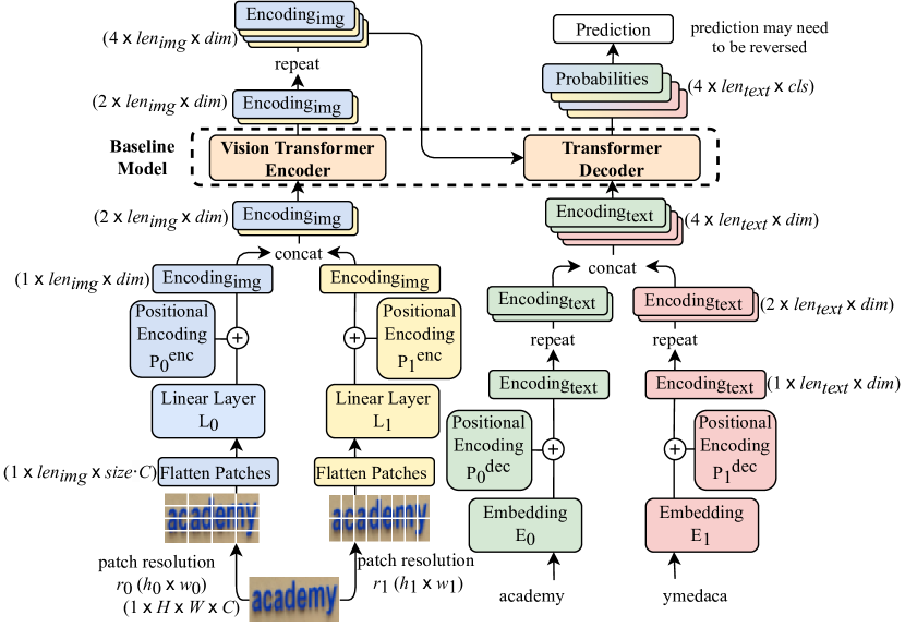
Figure 3: Architecture of PTIE. It is to be noted that there is no attention between the concatenated Encoding_img. This is also the case for concatenated Encoding_text. The attention is utilized as per vanilla transformer

4 Methodology

4.1 Model Architecture and Approach

Architecture of the proposed baseline model is illustrated in Fig. 3. It consists of a ViT encoder and a transformer decoder. Inspired by the mixture of experts, we present a transformer with integrated experts, named PTIE, to improve on the areas discussed in Section 3. Each expert, denoted as $Exp_{i,j}$, requires image patches of resolution $r_{i}$ and ground-truth texts of type $j$ to be trained where $i,j\in\{0,1\}$. For this work, patch resolution $r_{0}$ has the dimension of $h_{0}\times w_{0}=4\times 8$, and $r_{1}$ has that of $h_{1}\times w_{1}=8\times 4$. Both patch resolutions have the same patch size $size=h_{0}w_{0}=h_{1}w_{1}$. $j=0$ represents the use of original ground-truth texts (e.g. ‘academy’), and $j=1$ for reversed ground-truths (e.g. ‘ymedaca’).

For expert $Exp_{i,j}$, the resized image of dimension $H\times W\times C$ (height $\times$ width $\times$ channels) will first be split up into patches of resolution $r_{i}$ and then flatten. The sequence of flatten patches with length of $len_{img}$ is passed through linear layer $L_{i}$. The output, Encoding_img, will then be summed with positional encoding $P^{enc}_{i}$ before going through the encoder with encoding dimension of $dim$. Similarly, the ground-truths of type $j$ will go through an embedding layer $E_{j}$ and outputs Encoding_text with sequence length, $len_{text}$. It is then summed with $P^{dec}_{j}$ before being passed into the decoder which produces the probabilities over the total number of classes, $cls$. Cross-entropy loss will then be applied to the probabilities with their respective type $j$ ground-truths.

In our design, all experts are integrated into 1 model. The parameters in the encoder and decoder are shared. The differentiating factors among them are the initial linear/embedding layers as well as the positional encodings. More precisely, each expert shares about $96\%$ of the parameters with the others and each sample from the dataset will have 4 sets of input (1 for each expert), namely: (1) image split into patches of $4\times 8$ with the original ground-truth text, (2) $4\times 8$ patches with reversed ground-truth text, (3) $8\times 4$ patches with original ground-truth, and (4) $8\times 4$ patches with reversed ground-truth. It is to be noted that our baseline model mentioned in this work employs only 1 set of input (e.g. $i=0,j=0$: $4\times 8$ patches with original ground-truth).

The manipulation of the dimensions with repeat and concatenation depicted in Fig. 3 ensures that PTIE decodes each sample image only once despite having 4 sets of initial input. This will allow the inference latency to be close to that of the baseline model. As an ensemble-inspired method, the model will generate 4 predictions for a given sample. The output with the highest word probability (calculated by the multiplications of characters probability) will then be selected as the final prediction. However, different from a standard ensemble, our proposed model requires only a quarter of the parameters and inference time while remaining competitive against an ensemble of models in terms of accuracy.

4.2 Positional Encoding

According to the study by Ke et al [19], the positional encoding used in the vanilla transformer [37] causes noisy correlation with the embeddings of input tokens (e.g. characters) and may be detrimental to the model. Therefore, on top of the aforementioned proposed model, their strategy of untying the positional encoding from the input token embedding was also adopted.

Instead of summing the positional encoding, a positional attention is instead calculated and then added during the multi-head attention process. The positional attention for the encoder, $\alpha^{enc}_{i}$, is calculated as in Eq. 2:

$$\alpha^{enc}_{i}=\frac{1}{\sqrt{2d}}(P^{enc}_{i}W_{Q})(P^{enc}_{i}W_{K})^{T}$$ (2)

where $P^{enc}_{i}$ is the positional encoding of the patches with resolution $r_{i}$; $d$ is the dimension of positional encodings; $W_{Q}$ and $W_{K}$ are linear layers with the same number of input and output dimensions. All layers in the encoder share the $\alpha^{enc}_{i}$.

The decoder has masked self-attention and cross-attention layers. Their positional attentions, $\alpha^{dec}_{j}$ and $\alpha^{dec\_c}_{i,j}$, are calculated as in Eq. 3 and Eq. 4 respectively:

$$\alpha^{dec}_{j}=\frac{1}{\sqrt{2d}}(P^{dec}_{j}U_{Q})(P^{dec}_{j}U_{K})^{T}$$ (3)

$$\alpha^{dec\_c}_{i,j}=\frac{1}{\sqrt{2d}}(P^{dec}_{j}V_{Q})(P^{enc}_{i}V_{K})^{T}$$ (4)

where $i$ and $j$ denote the types of patch resolution and ground-truth and $U_{Q}$, $U_{K}$, $V_{Q}$, $V_{K}$ are linear layers like $W_{Q}$ and $W_{K}$. Similarly, all the layers in the decoder share the same positional attentions.

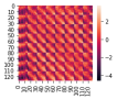
(a)

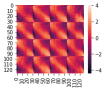
(b)

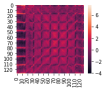
(c)

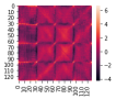
(d)

Figure 4: Learned unnormalized positional attention maps in the encoder of PTIE for (a) head 1, resolution=$4\times 8$; (b) head 1, resolution=$8\times 4$; (c) head 2, resolution=$4\times 8$; (d) head 2, resolution=$8\times 4$. The axes represent the indices of the flatten patches

The image patches of both resolutions were flatten in row-major order. With a large amount of parameters sharing, the spatial layouts of flatten patches with different patch resolutions for PTIE are handled by the positional encodings as shown in Fig. 4. Thus, the unnormalized positional attention maps for patch resolution $4\times 8$ and $8\times 4$ are different.

4.3 Implementation Details

The network was implemented using PyTorch and trained with ADAM optimizer with a base learning rate of $0.02$, betas of $(0.9,0.98)$, and eps of $1e^{-9}$, warmup duration of $6000$ steps with a decaying rate of $\min({steps^{-0.5}},steps\times warmup^{-1.5})$. The models were trained on $5$ NVIDIA RTX3090, with a batch size of $640$. All experiments were trained for $10$ epochs. Images are grayscaled and resized to a height and width of $32$ by $128$ without retaining the original aspect ratios. Standard augmentation techniques following Fang et al.’s work [8] were applied. The models in all experiments contain $6$ encoder layers and $6$ decoder layers with dropout of $0.1$. The encoding dimension is $512$ with $16$ heads for the multi-head attention. The feed forward layer has an intermediate dimension of $2048$. The model recognizes $100$ classes for training, including $10$ digits, $52$ case sensitive alphabets, $35$ punctuation characters, a start token, an end token, and a pad token. For testing, only $36$ case-insensitive alphanumeric characters were taken into consideration as per related works [35, 43, 8]. Greedy decoding was used with a maximum sequence length of $30$. No rotation strategy [21] was used.

5 Experimental Results and Analysis

5.1 Datasets

5.1.1 Synthetic datasets.

Two synthetic datasets were used: MJSynth (MJ) [16], with $9$ million samples, and SynthText (ST) [11], containing 8 million images. Some works utilized SynthAdd (SA) [21] due to the lack of punctuation in MJSynth and SynthText. SA was not used in our training.

5.1.2 Real datasets.

For evaluation, $6$ datasets of real scene text images which contain $7$ benchmarks were used. IIIT 5K-Words (IIIT5K) [26] contains $3000$ test images. ICDAR 2013 (IC13) [18] contains $1015$ testing images as per related work [39]. Two verions of ICDAR 2015 (IC15) [17] , containing $2077$ test images and $1811$ images, were used for evaluation. Street View Text (SVT) [39] consists of $647$ testing images. Street View Text-Perspective (SVT-P) [28] contains $645$ testing images. CUTE80 (CT) [32] contains $288$ test images. COCO-Text [10] which contains $42,618$ training images were used for fine-tuning so as to compare with works which uses real datasets in training or fine-tuning.

5.2 Comparison with State-of-the-Art Methods

Table 1: Comparison of accuracies on benchmark datasets with works trained using synthetic datasets. PTIE–Untied uses the learnable positional encoding discussed in Section 4.2 while PTIE–Vanilla uses it as per vanilla transformer method. The best and second best results as compared with PTIE–Untied are in bold and underline respectively. Values in the parenthesis are the difference in accuracy between the proposed model with the best or next best result. Note that the comparison of results are only between a PTIE-based model and other related works

Method	Year	Train	Regular Text			Irregular Text
		Datasets	IIIT	IC13	SVT	IC15		SVT-P	CT
			3000	1015	647	2077	1811	645	288
Luo et al. [24]	PR ‘19	ST+MJ	91.2	92.4	88.3	68.8	-	76.1	77.4
Yang et al. [44]	ICCV ‘19	ST+MJ	94.4	93.9	88.9	78.7	-	80.8	87.5
Zhan and Lu [47]	CVPR ‘19	ST+MJ	93.3	91.3	90.2	76.9	-	79.6	83.3
Wang et al. [40]	AAAI ‘20	ST+MJ	94.3	93.9	89.2	74.5	-	80.0	84.4
Wan et al. [38]	AAAI ‘20	ST+MJ	93.9	92.9	90.1	-	79.4	84.3	83.3
Zhang et al. [49]	ECCV ‘20	ST+MJ	94.7	94.2	90.9	-	81.8	81.7	-
Yue et al. [46]	ECCV ‘20	ST+MJ	95.3	94.8	88.1	77.1	-	79.5	90.3
Lee et al. [20]	CVPRW ‘20	ST+MJ	92.8	94.1	91.3	79.0	-	86.5	87.8
Yu et al. [45]	CVPR ‘20	ST+MJ	94.8	-	91.5	-	82.7	85.1	87.8
Qiao et al. [30]	CVPR ‘20	ST+MJ	93.8	92.8	89.6	80.0	-	81.4	83.6
Lu et al. [23]	PR ‘21	ST+MJ+SA	95.0	95.3	90.6	79.4	-	84.5	87.5
Raisi et al. [31]	CRV ‘21	ST+MJ	94.8	94.1	90.4	80.5	-	86.8	88.2
Qiao et al. [29]	ACMMM ‘21	ST+MJ	95.2	93.4	91.2	81.0	83.5	84.3	90.9
Atienza [1]	ICDAR ‘21	ST+MJ	88.4	92.4	87.7	72.6	78.5	81.8	81.3
Zhang et al. [48]	AAAI ‘21	ST+MJ	95.2	94.8	90.9	79.5	82.8	83.2	87.5
Wang et al. [41]	ICCV ‘21	ST+MJ	95.8	95.7	91.7	-	83.7	86.0	88.5
Wu et al. [42]	ICMR ‘21	ST+MJ	95.1	94.4	90.7	-	84.0	85.0	86.1
Fu et al. [9]	ICMR ‘21	ST+MJ	96.2	97.3	93.5	-	84.9	88.2	91.2
Zhang et al. [50]	ICMR ‘21	ST+MJ	90.3	96.8	89.5	76.0	-	78.5	78.9
Luo et al. [25]	IJCV ‘21	ST+MJ	95.6	96.0	92.9	81.4	83.9	85.1	91.3
Yan et al. [43]	CVPR ‘21	ST+MJ	95.6	-	94.0	-	83.0	87.6	91.7
Baek et al. [2]	CVPR ‘21	ST+MJ	92.1	93.1	88.9	74.7	-	79.5	78.2
Fang et al. [8]	CVPR ‘21	ST+MJ	96.2	97.4	93.5	-	86.0	89.3	89.2
PTIE–Vanilla		ST+MJ	96.7	97.1	95.5	83.4	87.4	89.8	91.3
			(+0.5)	(-0.3)	(+1.5)	(+2.0)	(+1.4)	(+0.5)	(-0.4)
PTIE–Untied		ST+MJ	96.3	97.2	94.9	84.3	87.8	90.1	91.7
			(+0.1)	(-0.2)	(+0.9)	(+2.9)	(+1.8)	(+0.8)	(0.0)

The results of PTIE are compared with recent works from top conferences and journals as shown in Table 1. PTIE achieves state-of-the-art results for most of the benchmarks, even though it has a simple architecture. In particular, PTIE–Untied attained the best results in $6$ out of $7$ benchmarks, outperforming the next best method by $0.9\%$ for SVT, $2.9\%$ for IC15 ($2077$), $1.8\%$ for IC15 ($1811$), and $0.8\%$ for SVTP. The model loses out to the best accuracy [8] on IC13 by $0.2\%$ and achieved the third highest accuracy. Similarly, PTIE–Vanilla attained the highest accuracy in $5$ benchmarks as compared with recent works. Fig. 5 shows examples of success and failure cases.

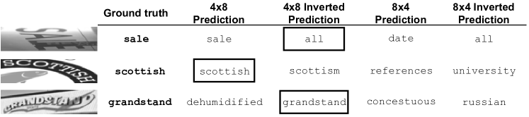
Figure 5: Sample images of success and failure cases. The boxed text represents final output from PTIE. More examples are in the supplementary material

Comparing with works that utilize real datasets, we fine-tune our PTIE models with real dataset (COCO-Text [10]) with results shown in Table 2. Through fine-tuning, our proposed model attained some improvement in performance. The model is able to outperform the state-of-the-art methods for $4$ of the benchmarks and achieved the second highest for $2$ bechmarks. Between the PTIE models trained with ST+MJ, PTIE–Untied has a weighted average (over the benchmarks) of $0.1\%$ higher than PTIE–Vanilla. For ST+MJ+R, PTIE–Untied has a weighted average of $0.4\%$ higher than PTIE–Vanilla.

Table 2: Comparison of accuracies on the benchmark datasets. The letter ‘R’ denotes the use of real dataset either in training or fine-tuning. The best and second best results in comparison with PTIE–Untied are in bold and underline respectively. Values in the parenthesis are the difference in accuracy between the proposed model with the best or next best result. Note that the comparison of results are only between a PTIE-based model and other related works

Method	Year	Train	Regular Text			Irregular Text
		Datasets	IIIT	IC13	SVT	IC15		SVT-P	CT
			3000	1015	647	2077	1811	645	288
Li et al. [21]	AAAI ‘19	ST+MJ+SA+R	95.0	94.0	91.2	78.8	-	86.4	89.6
Yue et al. [46]	ECCV ‘20	ST+MJ+R	95.4	94.1	89.3	79.2	-	82.9	92.4
Wan et al. [38]	AAAI ‘20	ST+MJ+R	95.7	94.9	92.7	-	83.5	84.8	91.6
Hu et al. [14]	AAAI ‘20	ST+MJ+SA+R	95.8	94.4	92.9	79.5	-	85.7	92.2
Qiao et al. [29]	ACMMM ‘21	ST+MJ+R	96.7	95.4	94.7	85.9	88.7	88.2	92.7
Baek et al. [2]	CVPR ‘21	R	93.5	92.6	87.5	76.0	-	82.7	88.1
Luo et al. [25]	IJCV ‘21	ST+MJ+R	96.5	95.6	94.4	84.7	87.2	86.2	92.4
PTIE–Vanilla		ST+MJ+R	96.5	96.1	96.3	84.5	89.0	91.3	88.5
			(-0.2)	(+0.5)	(+1.6)	(-1.4)	(+0.3)	(+3.1)	(-4.2)
PTIE–Untied		ST+MJ+R	96.6	96.6	95.8	85.1	89.2	92.1	91.0
			(-0.1)	(+1.0)	(+1.1)	(-0.8)	(+0.5)	(+3.9)	(-1.7)

5.3 Ablation Studies

5.3.1 Transformer-only Encoder.

In order to demonstrate the effectiveness of utilizing transformer-only encoder, 2 models were trained. We used a ViT encoder with transformer decoder as the baseline model and added a 45-layer ResNet [35] on top for the second model. Both models have the same hyperparameters. Comparison with works of similar architecture and method are given in Table 3.

Table 3: Comparison of accuracies with related works that are heavily based on transformer. The related works contain slight variations in the transformer architecture as discussed in Section 2. The reported accuracy is the weighted average over the $6$ benchmarks. The total count of $7672$ includes IC15 (2077) while $7406$ uses IC15 (1811). Note that Lee et al. [20] uses two convolutional layers

Method	Encoder	Decoder	Parameters	Accuracy
				7672	7406
Raisi et al. [31]	ResNet based + Trans.	Trans.	-	89.5	-
Lu et al. [23]	GCNet based	Trans.	-	89.3	-
Wu et al. [42]	GCNet based + Trans.	Trans.	-	-	90.7
Lee et al. [20]	CNN based + Trans.	Trans.	55.0M	88.4	-
	ResNet based + Trans.	Trans.	67.8M	85.7	87.1
	Vision Trans.	Trans.	45.8M	90.9	92.8

The transformer-only model outperforms the other works that employ a hybrid CNN-transformer encoder. This shows that competitive results can be achieved with just a pure transformer model. Furthermore, our experimental results show that adding a ResNet on top of the transformer encoder has a lower performance as compared with just using a vision transformer. Overall, the results suggest that exploiting the long-term dependency at an earlier stage in an encoder-decoder framework appears to be beneficial for STR.

5.3.2 Comparison with Standard Ensemble.

To evaluate the effectiveness of integrated experts, 4 separate models were each trained with one of the following inputs: (1) $8\times 4$ patches with original ground-truth, (2) $8\times 4$ patches with reversed ground-truth, (3) $4\times 8$ patches with original ground-truth, and (4) $4\times 8$ patches with reversed ground-truth. The ensemble of these 4 models is named Ensemble–Diverse and the PTIE trained with the 4 inputs is named PTIE–Diverse. The weighted average accuracies of the models over $6$ benchmarks are tabulated in Table 4. It is to be noted that untied positional encoding was used in all experiments of this section.

Table 4: Weighted average accuracies of mutilple methods on $6$ benchmark datasets (with $2077$ samples from IC15). The naming convention for the methods starts with the patch resolution (e.g. $8\times 4$) followed by the type of ground-truth used. “orig. GT” stands for the original ground-truth text, and “rev. GT” stands for the reversed ground-truth

Method	Parameters	Acc
		7672
$8\times 4$, orig. GT	45.8M	90.9
$8\times 4$, invt. GT	45.8M	90.0
$4\times 8$, orig. GT	45.8M	90.5
$4\times 8$, invt. GT	45.8M	90.1
Ensemble–Diverse	183.2M	92.4
$8\times 4$, orig. GT (1)	45.8M	90.9
$8\times 4$, orig. GT (2)	45.8M	90.7
$8\times 4$, orig. GT (3)	45.8M	90.5
$8\times 4$, orig. GT (4)	45.8M	90.7
Ensemble–Identical	183.2M	92.1
PTIE–Diverse	45.9M	92.4
PTIE–Identical	45.9M	91.0

Undoubtedly, the ensemble of the models brought about a significant performance boost. However, the improvement in accuracy comes at the price of requiring a greater amount of model parameters. Ensemble–Diverse needing $183.2$M parameters, achieved an accuracy of $92.4\%$. In contrast, PTIE–Diverse is able to achieve the same result of $92.4\%$ with only a quarter of the parameters.

The effectiveness of different patch resolutions and ground-truth types are also analyzed with 4 randomly initialized models trained with patch resolution of $8\times 4$ and original ground-truth. Their accuracies are shown in Table 4 together with their ensemble (Ensemble–Identical) and PTIE–Identical. Although there is only one type of ground-truth and patch resolution, PTIE–Identical is still trained with separate positional encoding, linear layers, and embedding layers as per Section 4.1. From the experimental results, accuracy of Ensemble–Identical is lower than that of Ensemble–Diverse by $0.3\%$ which highlights the effectiveness of using different resolutions and ground-truth types. Furthermore, PTIE–Identical suffers a 1.4% drop in accuracy indicating that different resolutions and ground-truth types are crucial for PTIE on leveraging the experts through different positional encoding, linear layers, and embedding layers.

5.3.3 Comparison of latency.

Table 5 shows a comparison of latency with other recent works that are open source. To tabulate the latency, inference on the test benchmarks was done with an RTX3090 and batch size of 1. Using 4 sets of well-designed inputs mentioned in Section 4.1, both PTIE–Diverse and Ensemble–Diverse achieved the highest average accuracy. Furthermore, the latency of 52ms by PTIE–Diverse is comparable to the baseline ($8\times 4$, orig. GT) and is a quarter of Ensemble–Diverse. This is because PTIE–Diverse decodes only once per sample despite having 4 sets of input, while Ensemble–Diverse needs to decode 4 times. MLT-19 [27] containing 10,000 real images for end-to-end scene recognition averages 11.2 texts instances per image. Using a batch size of 11, the latency of PTIE is about 11ms per cropped scene text image (averaging to 0.12s per full image). Therefore, it may not be a problem for real-time applications. Furthermore, in situations such as applications in forensic science (e.g. parsing images from suspect’s hard disk) or assistance to visually impaired, accuracy would be valued over latency.

Table 5: Inference time and weighted average accuracy of recent works. The total count of 7672 uses IC15 (2077) on top of the 5 other datasets mentioned in Section 5.1.1. 7406 uses IC15 (1811) and 7248 uses IC15 (1811) and a filtered version of IC13. The variation in total count is due to other works using varied set of benchmarks

Method	Year	Avg. accuracy			Parameters	Time
		7672	7406	7248	(mil.)	(ms)
Wang et al. [40]	AAAI ‘20	86.9	-	-	18.4	22
Lu et al. [23]	PR ‘21	89.3	-	-	54.6	53
Fang et al. [8]	CVPR ‘21	-	92.8	-	36.7	27
Yan et al. [43]	CVPR ‘21	-	-	91.5	29.1	29
$8\times 4$, orig. GT		90.9	92.8	92.2	45.8	50
Ensemble–Diverse		92.4	93.7	93.8	183.2	202
PTIE–Diverse		92.4	94.1	93.5	45.9	52

(a)

(b)

Figure 6: Relative frequency distribution change in correct predictions of (a) PTIE from model trained with resolution $4\times 8$ and original ground-truth. (b) PTIE from model trained with resolution $8\times 4$ and original ground-truth

5.4 Addressing Areas for Improvement

As per Section 3.1, the relative frequency distribution changes of PTIE–Diverse from the models trained with (1) $4\times 8$ patches and (2) $8\times 4$ patches, are plotted in Fig. 6a and Fig. 6b respectively. Relative improvement in the predictions is seen in most of the lengths and scales for both patch resolutions. This shows that PTIE is effective in utilizing the advantages of both resolutions.

Furthermore, the frequency distributions in Fig. 7 demonstrate that PTIE–Diverse, trained with original and reversed ground-truth, is able to lower the prediction error of first character as discussed in Section 3.2. Overall, PTIE is able to improve the accuracy in STR by mitigating the problem of the weak first character prediction. Non-autoregressive decoding is explored in the supplementary material.

(a)

(b)

Figure 7: Normalized frequency distributions of wrong predictions by PTIE for word length $5$ conditioned on ground truth characters. (a) Predictions with one wrong character. (b) Predictions with two wrong characters

6 Conclusion

In this work, a simple and strong transformer-only baseline was introduced. By exploiting the long-term dependency of STR at an earlier stage in the model, the baseline is able to outperform related works which uses hybrid transformer. We then analyzed and discussed two areas for improvement for transformer in STR. The integrated experts method was proposed to address them and state-of-the-art results were attained for most benchmarks. As the final predictions of PTIE were selected based on word probability, we will explore more selection methods and streamline the processes in PTIE for future work.

Acknowledgments: This work is partially supported by NTU Internal Funding - Accelerating Creativity and Excellence (NTU–ACE2020-03).

References

- [1] Atienza, R.: Vision transformer for fast and efficient scene text recognition. ICDAR (2021)
- [2] Baek, J., Matsui, Y., Aizawa, K.: What if we only use real datasets for scene text recognition? toward scene text recognition with fewer labels. In: CVPR. pp. 3113–3122 (2021)
- [3] Bartz, C., Bethge, J., Yang, H., Meinel, C.: Kiss: Keeping it simple for scene text recognition. arXiv preprint arXiv:1911.08400 (2019)
- [4] Cao, Y., Xu, J., Lin, S., Wei, F., Hu, H.: Gcnet: Non-local networks meet squeeze-excitation networks and beyond. In: ICCVW. pp. 0–0 (2019)
- [5] Chen, X., Jin, L., Zhu, Y., Luo, C., Wang, T.: Text recognition in the wild: A survey. ACM Comput. Surv. 54(2), 1–35 (2021)
- [6] Dosovitskiy, A., Beyer, L., Kolesnikov, A., Weissenborn, D., Zhai, X., Mostafa, T., Dehghani, M., Minderer, M., Heigold, G., Gelly, S., Uszkoreit, J., Houlsby, N.: An image is worth 16x16 words: Transformers for image recognition at scale. In: ICLR (2021)
- [7] Ezaki, N., Kiyota, K., Minh, B.T., Bulacu, M., Schomaker, L.: Improved text-detection methods for a camera-based text reading system for blind persons. In: ICDAR. pp. 257–261 (2005)
- [8] Fang, S., Xie, H., Wang, Y., Mao, Z., Zhang, Y.: Read like humans: Autonomous, bidirectional and iterative language modeling for scene text recognition. In: CVPR. pp. 7098–7107 (2021)
- [9] Fu, Z., Xie, H., Jin, G., Guo, J.: Look back again: Dual parallel attention network for accurate and robust scene text recognition. In: ICMR. pp. 638–644 (2021)
- [10] Gomez, R., Shi, B., Gomez, L., Numann, L., Veit, A., Matas, J., Belongie, S., Karatzas, D.: Icdar 2017 robust reading challenge on coco-text. In: ICDAR. vol. 1, pp. 1435–1443 (2017)
- [11] Gupta, A., Vedaldi, A., Zisserman, A.: Synthetic data for text localisation in natural images. In: CVPR. pp. 2315–2324 (2016). https://doi.org/10.1109/CVPR.2016.254
- [12] Gurari, D., Li, Q., Stangl, A.J., Guo, A., Lin, C., Grauman, K., Luo, J., Bigham, J.P.: Vizwiz grand challenge: Answering visual questions from blind people. In: CVPR. pp. 3608–3617 (2018)
- [13] Hochreiter, S., Schmidhuber, J.: Long short-term memory. Neural computation 9(8), 1735–1780 (1997)
- [14] Hu, W., Cai, X., Hou, J., Yi, S., Lin, Z.: Gtc: Guided training of ctc towards efficient and accurate scene text recognition. In: AAAI. vol. 34, pp. 11005–11012 (2020)
- [15] Huang, D., Lang, Y., Liu, T.: Evolving population distribution in china’s border regions: Spatial differences, driving forces and policy implications. Plos one 15(10), e0240592 (2020)
- [16] Jaderberg, M., Simonyan, K., Vedaldi, A., Zisserman, A.: Synthetic data and artificial neural networks for natural scene text recognition. arXiv preprint arXiv:1406.2227 (2014)
- [17] Karatzas, D., Gomez-Bigorda, L., Nicolaou, A., Ghosh, S., Bagdanov, A., Iwamura, M., Matas, J., Neumann, L., Chandrasekhar, V.R., Lu, S., et al.: Icdar 2015 competition on robust reading. In: ICDAR. pp. 1156–1160 (2015)
- [18] Karatzas, D., Shafait, F., Uchida, S., Iwamura, M., i Bigorda, L.G., Mestre, S.R., Mas, J., Mota, D.F., Almazan, J.A., De Las Heras, L.P.: Icdar 2013 robust reading competition. In: ICDAR. pp. 1484–1493 (2013)
- [19] Ke, G., He, D., Liu, T.Y.: Rethinking positional encoding in language pre-training. In: ICLR (2020)
- [20] Lee, J., Park, S., Baek, J., Oh, S.J., Kim, S., Lee, H.: On recognizing texts of arbitrary shapes with 2d self-attention. In: CVPRW. pp. 546–547 (2020)
- [21] Li, H., Wang, P., Shen, C., Zhang, G.: Show, attend and read: A simple and strong baseline for irregular text recognition. In: AAAI. vol. 33, pp. 8610–8617 (July 2019)
- [22] Long, S., He, X., Yao, C.: Scene text detection and recognition: The deep learning era. IJCV 129(1), 161–184 (2021)
- [23] Lu, N., Yu, W., Qi, X., Chen, Y., Gong, P., Xiao, R., Bai, X.: Master: Multi-aspect non-local network for scene text recognition. PR 117, 107980 (2021)
- [24] Luo, C., Jin, L., Sun, Z.: Moran: A multi-object rectified attention network for scene text recognition. PR 90, 109–118 (2019)
- [25] Luo, C., Lin, Q., Liu, Y., Jin, L., Shen, C.: Separating content from style using adversarial learning for recognizing text in the wild. IJCV 129(4), 960–976 (2021)
- [26] Mishra, A., Alahari, K., Jawahar, C.: Scene text recognition using higher order language priors. In: BMVC (2012)
- [27] Nayef, N., Patel, Y., Busta, M., Chowdhury, P.N., Karatzas, D., Khlif, W., Matas, J., Pal, U., Burie, J.C., Liu, C.l., et al.: Icdar2019 robust reading challenge on multi-lingual scene text detection and recognition—rrc-mlt-2019. In: ICDAR. pp. 1582–1587. IEEE (2019)
- [28] Phan, T.Q., Shivakumara, P., Tian, S., Tan, C.L.: Recognizing text with perspective distortion in natural scenes. In: ICCV. pp. 569–576 (2013). https://doi.org/10.1109/ICCV.2013.76
- [29] Qiao, Z., Zhou, Y., Wei, J., Wang, W., Zhang, Y., Jiang, N., Wang, H., Wang, W.: Pimnet: A parallel, iterative and mimicking network for scene text recognition. In: ACMMM. pp. 2046–2055 (2021)
- [30] Qiao, Z., Zhou, Y., Yang, D., Zhou, Y., Wang, W.: Seed: Semantics enhanced encoder-decoder framework for scene text recognition. In: CVPR (June 2020)
- [31] Raisi, Z., Naiel, M.A., Younes, G., Wardell, S., Zelek, J.: 2lspe: 2d learnable sinusoidal positional encoding using transformer for scene text recognition. In: CRV. pp. 119–126 (2021)
- [32] Risnumawan, A., Shivakumara, P., Chan, C.S., Tan, C.L.: A robust arbitrary text detection system for natural scene images. Expert Systems with Applications 41(18), 8027–8048 (2014). https://doi.org/https://doi.org/10.1016/j.eswa.2014.07.008, https://www.sciencedirect.com/science/article/pii/S0957417414004060
- [33] Schulz, R., Talbot, B., Lam, O., Dayoub, F., Corke, P., Upcroft, B., Wyeth, G.: Robot navigation using human cues: A robot navigation system for symbolic goal-directed exploration. In: ICRA. pp. 1100–1105 (2015)
- [34] Shi, B., Bai, X., Yao, C.: An end-to-end trainable neural network for image-based sequence recognition and its application to scene text recognition. PAMI 39(11), 2298–2304 (2016)
- [35] Shi, B., Yang, M., Wang, X., Lyu, P., Yao, C., Bai, X.: Aster: An attentional scene text recognizer with flexible rectification. PAMI 41(9), 2035–2048 (2018)
- [36] Tsai, S.S., Chen, H., Chen, D., Schroth, G., Grzeszczuk, R., Girod, B.: Mobile visual search on printed documents using text and low bit-rate features. In: ICIP. pp. 2601–2604 (2011)
- [37] Vaswani, A., Shazeer, N., Parmar, N., Uszkoreit, J., Jones, L., Gomez, A.N., Kaiser, Ł., Polosukhin, I.: Attention is all you need. In: NIPS. vol. 30 (2017)
- [38] Wan, Z., He, M., Chen, H., Bai, X., Yao, C.: Textscanner: Reading characters in order for robust scene text recognition. In: AAAI. vol. 34, pp. 12120–12127 (April 2020)
- [39] Wang, K., Babenko, B., Belongie, S.: End-to-end scene text recognition. In: ICCV. pp. 1457–1464 (2011)
- [40] Wang, T., Zhu, Y., Jin, L., Luo, C., Chen, X., Wu, Y., Wang, Q., Cai, M.: Decoupled attention network for text recognition. In: AAAI. vol. 34, pp. 12216–12224 (April 2020). https://doi.org/10.1609/aaai.v34i07.6903
- [41] Wang, Y., Xie, H., Fang, S., Wang, J., Zhu, S., Zhang, Y.: From two to one: A new scene text recognizer with visual language modeling network. In: ICCV. pp. 14194–14203 (2021)
- [42] Wu, L., Liu, X., Hao, Y., Ma, Y., Hong, R.: Naster: Non-local attentional scene text recognizer. In: ICMR. pp. 331–338 (2021)
- [43] Yan, R., Peng, L., Xiao, S., Yao, G.: Primitive representation learning for scene text recognition. In: CVPR. pp. 284–293 (2021)
- [44] Yang, M., Guan, Y., Liao, M., He, X., Bian, K., Bai, S., Yao, C., Bai, X.: Symmetry-constrained rectification network for scene text recognition. In: ICCV (October 2019)
- [45] Yu, D., Li, X., Zhang, C., Liu, T., Han, J., Liu, J., Ding, E.: Towards accurate scene text recognition with semantic reasoning networks. In: CVPR. pp. 12113–12122 (2020)
- [46] Yue, X., Kuang, Z., Lin, C., Sun, H., Zhang, W.: Robustscanner: Dynamically enhancing positional clues for robust text recognition. In: ECCV. pp. 135–151. Cham (2020)
- [47] Zhan, F., Lu, S.: Esir: End-to-end scene text recognition via iterative image rectification. In: CVPR (June 2019)
- [48] Zhang, C., Xu, Y., Cheng, Z., Pu, S., Niu, Y., Wu, F., Zou, F.: Spin: Structure-preserving inner offset network for scene text recognition. In: AAAI. vol. 35, pp. 3305–3314 (2021)
- [49] Zhang, H., Yao, Q., Yang, M., Xu, Y., Bai, X.: Autostr: Efficient backbone search for scene text recognition. In: ECCV. pp. 751–767 (2020)
- [50] Zhang, M., Ma, M., Wang, P.: Scene text recognition with cascade attention network. In: ICMR. pp. 385–393 (2021)