Black-Box Model Confidence Sets Using Cross-Validation with High-Dimensional Gaussian Comparison

Nicholas Kissel Carnegie Mellon University Jing Lei Carnegie Mellon University
Abstract

We derive high-dimensional Gaussian comparison results for the standard $V$-fold cross-validated risk estimates. Our results combine a recent stability-based argument for the low-dimensional central limit theorem of cross-validation with the high-dimensional Gaussian comparison framework for sums of independent random variables. These results give new insights into the joint sampling distribution of cross-validated risks in the context of model comparison and tuning parameter selection, where the number of candidate models and tuning parameters can be larger than the fitting sample size. As a consequence, our results provide theoretical support for a recent methodological development that constructs model confidence sets using cross-validation.

1 Introduction

Cross-validation (Stone, 1974; Allen, 1974; Geisser, 1975) is among the most popular procedures for estimating the out-of-sample predictive performance of statistical models fitted on data sets randomly sampled from a population. Generally speaking, cross-validation estimates the out-of-sample prediction accuracy by fitting and assessing a fitted model on separate subsets of data. One of the most common forms of cross-validation is $V$-fold cross-validation, where data are partitioned into $V$ folds (sets) of identical size; then, each fold is used to assess the error of the model fitted using the other $V-1$ folds. Finally, the average of all $V$ estimates is used to create the cross-validation risk estimate.

Cross-validation is commonly used in statistical learning problems wherein researchers either compare the cross-validated risk of multiple models or compare a cross-validated risk against some baseline method with known risk. See Picard and Cook (1984); Arlot and Celisse (2010) for examples. The popularity and simplicity of cross-validation has inspired numerous research articles seeking to better understand its theoretical properties. In particular, positive results have been established for parameter estimation following the model selected by cross-validation, including risk consistency and parameter estimation consistency. See Stone (1977b); Homrighausen and McDonald (2017); Chetverikov etย al. (2016); Celisse (2014) for various examples from linear regression to nonparametric density estimation problems.

Despite the consistency results established for parameter estimation, understanding the model selection properties of cross-validation has been a challenging task, with most existing results being negative. In the early work of Stone (1977a), it is shown that cross-validation is similar to AIC, and hence prone to choosing overfitted linear regression models. Such an overfitting tendency of cross-validation has been further studied in Shao (1993); Zhang (1993); Yang (2007), which show that in the classical regime, cross-validation often produces inconsistent model selection unless a very unrealistic train-validate ratio is used. Indeed, these ratios are so extreme that they can never be satisfied by standard V-fold cross-validation. Furthermore, the unsatisfactory model selection performance of cross-validation has been widely observed in practice, and many heuristic or context-specific adjustments have been proposed, such as Efron and Tibshirani (1997); Tibshirani and Tibshirani (2009); Yu and Feng (2014).

The model selection inconsistency of cross-validation can be understood as an instance of the โ€œwinnerโ€™s curse.โ€ Since the cross-validated risk of each model is still a random variable, a particular model may have the smallest cross-validated risk because its realized random fluctuation happens to be small while the true optimal model has a much larger fluctuation. Such an intuition calls for a more precise understanding of the sampling distribution of cross-validated risks. A main challenge in studying the sampling distribution of cross-validated risk is the global and heterogeneous dependence among each individual empirical loss function. Bousquet and Elisseeff (2002) proved convergence of cross-validated risk to the corresponding population quantity under an expected leave-one-out loss stability condition. The population target of cross-validated risk and its variability is further studied in Bates etย al. (2021).

In this work, we study the simultaneous fluctuations of the cross-validated risks of many models around their mean values. In particular, we establish high-dimensional Gaussian comparison results for the cross-validated risk vector indexed by a collection of models, whose cardinality can potentially be very large. Our main contributions are two fold. First, we extend the low-dimensional central limit theorem by Austern and Zhou (2020) to the high-dimensional case, combining their cross-validation error analysis with the high-dimensional Gaussian comparison framework by Chernozhukov etย al. (2013). Second, we provide theoretically justifiable model selection confidence sets using cross-validation, answering an open question left in the methodological work Lei (2020).

Our theoretical development extends and merges two lines of current research: central limit theorems for cross-validation and high-dimensional Gaussian comparisons. Low-dimensional central limit theorems for cross-validation have been developed recently by Austern and Zhou (2020) and Bayle etย al. (2020). While these low-dimensional results provide very useful insights for the estimation of prediction risks of individual models, they cannot be used to construct simultaneous confidence sets when many candidate models are being compared. This is of particular interest because in practice, cross-validation is often used to compare and select from a large collection of models or tuning parameters. Therefore, in order to understand the behavior of cross-validation in selecting from many models, it is necessary to consider the joint sampling distribution of the cross-validated risks. In the case of sums of independent random vectors, high-dimensional Gaussian comparison has been developed in the milestone work of Chernozhukov etย al. (2013) (see also Bentkus, 2005). Since then, similar results have been developed for $U$-statistics (Chen, 2018) and stochastic processes with weak dependence such as mixing or spatial process (Kurisu etย al., 2021; Chang etย al., 2021). However, these extensions do not cover the cross-validation case, where all terms in the summation are dependent on each other and have similar magnitudes of dependence, violating the sparsity of dependence ($U$-statistics) and fast decaying dependence (mixing and spatial processes). In fact, a different extension of the Gaussian comparison result is needed for cross-validation, which borrows the martingale decomposition and stability conditions in Austern and Zhou (2020).

Stability conditions play a key role in developing the Gaussian comparison results in this work. Outside of the analysis of cross-validation, the importance of stability has been studied in the broader statistics and machine learning communities (Yu, 2013; Meinshausen and Bรผhlmann, 2010; Bousquet and Elisseeff, 2002; Hardt etย al., 2016). To develop our results, we require more subtle versions of stability than in the existing literature, including second order stability, stability in sub-Weibull tails, and stability of difference loss functions. We provide rigorous justifications of these stability conditions for the stochastic gradient descent algorithm and a prototypical non-parametric regression setting.

2 Preliminaries

Consider iid data $\mathbf{X}=(X_{0},X_{1},...,X_{n})$ with $X_{i}\in\mathcal{X}$. We would like to simultaneously study the performance of $p$ learning algorithms through the framework of $V$-fold cross-validation.

For notation simplicity, we assume $V$ evenly divides $n$. For $v\in[V]$, let $I_{v}=\{n(v-1)/V+1,...,nv/V\}$ be the index that corresponds to the $v$th fold of data. Let $\tilde{n}=n(1-1/V)$ be the training sample size used in $V$-fold cross-validation. For each $r\in[p]$, let $\ell_{r}(\cdot;\cdot):\mathcal{X}\times\mathcal{X}^{\tilde{n}}\mapsto\mathbb{R}$ be a loss function. Intuitively, we should think $\ell_{r}(x_{0};(x_{1},...,x_{\tilde{n}}))$ as the loss function evaluated at $x_{0}$ of a fitted model using training data $(x_{1},...,x_{\tilde{n}})$. Here the index $r$ denotes a particular model or tuning parameter value. This notation covers both supervised and unsupervised learning.

  1. 1.

    In supervised learning, each point can be thought of as $x=(y,z)\in\mathcal{Y}\times\mathcal{Z}$ where $z$ is a vector of covariates and $y$ is the response variable. The loss function can often be written more concretely as

    $$\ell_{r}(x_{0};(x_{1},...,x_{\tilde{n}}))=\rho(y_{0},\hat{f}_{r}(z_{0}))\,,$$

    where $\hat{f}_{r}(\cdot):\mathcal{Z}\mapsto\mathcal{Y}$ is a regression function that predicts $y$ from $z$, trained using the $r$th model/tuning parameter with input data $(x_{1},...,x_{\tilde{n}})$, and $\rho(\cdot,\cdot):\mathcal{Y}^{2}\mapsto\mathbb{R}$ is a loss function measuring the quality of predicting $y$ using $\hat{f}_{r}(z)$, such as squared loss, 00-$1$ loss, and hinge loss.

  2. 2.

    In unsupervised learning,

    $$\ell_{r}(x_{0};(x_{1},...,x_{\tilde{n}}))=\rho(x_{0};\hat{f}_{r})\,,$$

    where $\hat{f}_{r}$ is a function describing the distribution of $X$ trained from the $r$th model/tuning parameter with the input data $(x_{1},...,x_{\tilde{n}})$, and the function $\rho$ is a loss function assessing the agreement of the sample point $x_{0}$ and the fitted probability model $\hat{f}_{r}$. Examples of $\rho$ include the negative likelihood in density estimation and the proportion of total variance explained in dimension reduction.

In model selection and parameter tuning, a particularly interesting scenario is when the number of models being compared is large.

For each $r$, the $V$-fold cross-validated risk is

$$\hat{R}_{{\rm cv},r}=n^{-1}\sum_{i=1}^{n}\ell_{r}(X_{i};\mathbf{X}_{-v_{i}})\,.$$ (1)

where $\mathbf{X}_{-v}$ denotes the sub-vector of $\mathbf{X}$ excluding the $v$th fold, and $v_{i}\in[V]$ is such that $i\in I_{v_{i}}$.

It is natural to expect $\hat{R}_{{\rm cv},r}$ to approximate the true average risk of the fitted model:

$$\tilde{R}_{r}=\frac{1}{V}\sum_{v=1}^{V}R_{r}(\mathbf{X}_{-v})\,,$$

where

$$\tilde{R}_{r}(\mathbf{X}_{-v})=\mathbb{E}\left[\ell_{r}(X_{0};\mathbf{X}_{-v})|\mathbf{X}_{-v}\right]\,,$$

is the true risk of the $r$th model fitted using input data $\mathbf{X}_{-v}$.

The quantity $\tilde{R}_{r}(\mathbf{X}_{-v})$ still depends on the input data $\mathbf{X}_{-v}$ and hence is a random variable itself. It would be natural to consider its expected value

$$R_{r}^{*}=\mathbb{E}\tilde{R}_{r}(\mathbf{X}_{-v})=\mathbb{E}\ell_{r}(X_{0};\mathbf{X}_{-1})\,.$$

As a statistical inference task, model comparison also involves uncertainty quantification of risk point estimates, and one would hope to establish central limit theorems of the form

$$\frac{\sqrt{n}(\hat{R}_{{\rm cv},r}-\mu_{r})}{\sigma_{r}}\rightsquigarrow N(0,1)$$

with $\mu_{r}$ being either $\tilde{R}_{r}$ or $R_{r}^{*}$ and some appropriate scaling $\sigma_{r}$ (Austern and Zhou, 2020; Bayle etย al., 2020).

In the context of model comparison or tuning parameter selection, these individual normal approximations would have limited practical use. For example, in our numerical example in Sectionย 4.1, individual confidence intervals fail to simultaneously cover the targets when when $p$ is moderately large. To cover this gap between theory and practice, we seek to establish a high-dimensional Gaussian approximation in a similar fashion as in Chernozhukov etย al. (2013):

$$\sup_{z\in\mathbb{R}}\left|\mathbb{P}\left(\max_{1\leq r\leq p}\sqrt{n}(\hat{R}_{{\rm cv},r}-\mu_{r})\leq z\right)-\mathbb{P}\left(\max_{1\leq r\leq p}Y_{r}\leq z\right)\right|\rightarrow 0$$ (2)

for some centered Gaussian random vector $\mathbf{Y}=(Y_{1},...,Y_{p})$ with matching covariance.

3 Main results

In this section, we establish a high-dimensional Gaussian approximation result with random centering. In particular, we prove (2) with $\mu_{r}=\tilde{R}_{r}$. In the following subsections, we present and discuss the assumptions required for this result and provide its full statement as a theorem in Sectionย 3.3.

3.1 Symmetry and moment conditions on the loss function

The idea of cross-validation relies on independence and symmetry among data points. We consider the following symmetry and moment conditions on the loss functions $\ell_{r}$.

Assumption 1 (Symmetry and moment condition on $\ell_{r}$).

For each $r\in[p]$, the loss function $\ell_{r}(\cdot;\cdot)$ satisfies

  1. (a)

    $\ell_{r}(x_{0};x_{1},...,x_{\tilde{n}})$ is symmetric in $(x_{1},...,x_{\tilde{n}})$.

  2. (b)

    $\mathbb{E}\left\{[\ell_{r}(X_{1};\mathbf{X}_{-1})-R_{r}(\mathbf{X}_{-1})]^{2}\right\}\geq\underline{\sigma}^{2}$ for some constant $0<\underline{\sigma}$.

Part (b) essentially assumes that the randomly centered cross-validated loss function has non-degenerate conditional variance. This makes intuitive sense, as we would expect the resulting confidence interval to have length at the scale of $1/\sqrt{n}$. For example, if $\ell_{r}$ is a regression residual, then this lower bound is at least as large as the prediction risk of the ideal regression function. In the additional assumptions below, we will also have the upper bound on the variance term.

3.2 Stability and tail conditions

A key consideration from Austern and Zhou (2020) in their low dimensional central limit theorems for cross-validation is the stability of the loss function and the average risk when one input sample point is replaced by an iid copy. In the high dimensional case, we need the loss function to be stable in a uniform sense across all $p$ candidate models indexed by $r\in[p]$. Thus, we will consider stability conditions in the form of stronger tail inequalities instead of the moment conditions used for the low dimensional case. Such stronger tail conditions are common in high dimensional central limit theorem literature, such as in Chernozhukov etย al. (2013).

We use sub-Weibull concentration to describe the required tail behaviors of random variables.

Definition 1 (Sub-Weibull Random Variables).

Let $K$ be a positive number, we say a random variable $X$ is $K$-sub-Weibull ($K$-SW for short) if there are positive constants $(a,b,\alpha)$ such that

$$\mathbb{P}\left(\frac{|X|}{K}\geq t\right)\leq ae^{-bt^{\alpha}}\,,~{}~{}\forall~{}t>0\,.$$

This definition generalizes the well-known sub-exponential and sub-Gaussian distributions, and has been systematically introduced in Vladimirova etย al. (2020); Kuchibhotla and Chakrabortty (2018).

Remark 1.

Unlike common practices in the literature, our notation of the sub-Weibull tail inequality only focuses on the scaling $K$. We do not keep track of the constants $a,b,\alpha$, which can vary from one instance to another as long as they stay bounded and bounded away from zero. It is easy to check that our notion of sub-Weibull is invariant under constant scaling: if $X$ is $1$-SW, then $X$ is $c$-SW for all positive constant $c$. Aside from the scaling $K$, the second (and only) important parameter in sub-Weibull tail inequality is the exponent $\alpha$. In the literature, it is more common to write $(K,\alpha)$-SW. Our proof can be adapted to keep explicit track of the constant $\alpha$ in each instance at the cost of more complicated bookkeeping, but that does not qualitatively change the results.

In our theoretical developments, the dependence on logarithm terms may be complicated, as it involves the sub-Weibull constant $\alpha$, which may vary between lines. For brevity of presentation, we absorb such logarithm terms into the $\tilde{O}(\cdot)$ notation. Where $A\leq\tilde{O}(B)$ means that there are positive constants $c_{1},c_{2}$ independent of $(n,p)$ such that $A\leq c_{1}\log^{c_{2}}(n+p)B$.

To introduce the stability conditions, let $X_{i}^{\prime}$ be iid copies of $X_{i}$ for $1\leq i\leq n$ and $\mathbf{X}^{i}$ be the vector obtained by replacing $X_{i}$ with $X_{i}^{\prime}$. For any function $f(\mathbf{X})$, define $\nabla_{i}f(\mathbf{X})=f(\mathbf{X})-f(\mathbf{X}^{i})$.

The main stability conditions involved in our normal approximation bounds are the following.

Assumption 2.

There exists $\epsilon_{\ell}=n^{-c_{\ell}}$ for some $c_{\ell}\in(0,1/2]$ such that

  1. (a)

    For all $i\in[\tilde{n}]$, $r\in[p]$, $\nabla_{i}\ell_{r}(X_{0},\mathbf{X}_{-1})$ is $n^{-1/2}\epsilon_{\ell}$-sub-Weibull.

  2. (b)

    For all $1\leq i<j\leq\tilde{n}$, $r\in[p]$, $\nabla_{j}\nabla_{i}\ell_{r}(X_{0},\mathbf{X}_{-1})$ is $n^{-3/2}\epsilon_{\ell}$-sub-Weibull.

  3. (c)

    For all $r$, $\ell_{r}(X_{0},\mathbf{X}_{-1})$ is $1$-sub-Weibull.

Assumptionย 2 requires that the first order difference $\nabla_{i}\ell_{r}(X_{0},\mathbf{X}_{-1})$ has a scaling no larger than $\epsilon_{\ell}n^{-1/2}$, the second order difference $\nabla_{j}\nabla_{i}\ell_{r}(X_{0},\mathbf{X}_{-1})$ has a scaling no larger than $\epsilon_{\ell}n^{-3/2}$, and the original loss function $\ell_{r}$ has a constant scaling. The sub-Weibull tail ensures that with high probability all such quantities will not exceed their scalings by more than a poly-logarithm factor. We require $\epsilon_{\ell}\in[n^{-1/2},1)$, as this simplifies the presentation of the results and is also the most natural range of stability. Specifically, the approximation error bounds in our main theorems become meaningless if $\epsilon_{\ell}>1$, and $\epsilon_{\ell}\ll n^{-1/2}$ would be impractical, as it implies changing one sample point will incur a change less than $1/n$ in the loss.

We further remark that the scaling assumption on the second order difference $\nabla_{j}\nabla_{i}\ell_{r}(X_{0},\mathbf{X}_{-1})$ is stronger than that in Austern and Zhou (2020) by a factor of $\sqrt{n}$. This is due to a fundamental difference between the low dimensional CLT and high dimensional Gaussian comparison, where the former only requires controlling the second moment of error terms, while the latter requires controlling the supremum of many such error terms. More specifically, define the randomly centered loss at $X_{i}$

$$K_{r,i}=\ell_{r}(X_{i};\mathbf{X}_{-v_{i}})-R_{r}(\mathbf{X}_{-v_{i}})\,,$$ (3)

and

$$D_{r,i}=\sum_{j\notin I_{v_{i}}}\nabla_{i}K_{r,i}\,.$$ (4)

A key result in the low dimensional CLT is that $\|D_{r,i}\|_{2}\lesssim\epsilon_{\ell}$ provided $\|n^{1/2}\nabla_{i}\ell_{r}(X_{0},\mathbf{X}_{-1})\|_{2}\allowbreak\leq\epsilon_{\ell}$ and $n\|\nabla_{j}\nabla_{i}\ell_{r}(X_{0},\mathbf{X}_{-1})\|_{2}\leq\epsilon_{\ell}$. However, in the high-dimensional regime, we need to simultaneously control $D_{r,i}$ for all $1\leq r\leq p$, which cannot be guaranteed by a vanishing second moment on each individual term. Our condition can be relaxed to requiring a similar $\nabla_{j}\nabla_{i}\ell_{r}(X_{0},\mathbf{X}_{-1})$ being $n^{-1}\epsilon_{\ell}$-sub-Weibull, provided we can further assume that $\frac{D_{r,i}}{\|D_{r,i}\|_{2}}$ is $1$-sub-Weibull. While this additional assumption certainly seems reasonable in many situations, we choose to work with the stronger condition on the second order difference as presented in Assumptionย 2, which allows for a more streamlined presentation. Nevertheless, the stability conditions in Assumptionย 2 are still practically plausible since we should typically expect each $\nabla$ operator to reduce the scale of the loss function by a factor up to $n$.

In Sectionย 5, we provide two rigorous examples that satisfy the stability conditions, including stochastic gradient descent with convex and smooth objective functions, and a non-parametric regression with sub-Weibull design.

Example 1 (Classical M-Estimator).

Consider a parametric loss function $\ell(x_{0};x_{1},...,x_{\tilde{n}})=\ell(x_{0};\hat{\theta})$ with $\hat{\theta}$ estimated from the input data $(x_{1},...,x_{\tilde{n}})$. Under classical parametric regularity conditions such $\hat{\theta}$ can be asymptotically linear (Tsiatis, 2006, Chapter 3). Then we have

$$\hat{\theta}=\theta_{0}+\frac{1}{\tilde{n}}\sum_{i=1}^{\tilde{n}}\varphi(x_{i})+o_{P}(n^{-1/2})\,.$$

Intuitively, the first order stability bound for $\nabla_{i}\ell$ can be satisfied if the $o_{P}(n^{-1/2})$ remainder term is $n^{-1/2}\epsilon_{\ell}$-SW for some $\epsilon_{\ell}=o(1)$. The second order stability condition would require more subtle structure within the $o_{P}(n^{-1/2})$ remainder term. Austern and Zhou (2020) gave a formal analysis of the first and second order statbility conditions for $M$-estimators under convexity and smoothness.

Example 2 (Penalized Least Squares).

Now consider a high dimensional ridge-regression where we have paired sample points $x_{i}=(z_{i},y_{i})$:

$$\hat{\beta}=\arg\min{\tilde{n}}^{-1}\sum_{i=1}^{\tilde{n}}(y_{i}-z_{i}^{T}\beta)^{2}+\lambda\|\beta\|_{2}^{2}\,.$$

When the dimensionality of $x_{i}$ is comparable or smaller than the sample size, it is possible to argue that the empirical covariance matrix will be well-conditioned with high probability, and hence changing any one sample point will incur an $O(n^{-1})$ change in $\hat{\beta}$. For a simpler argument under stronger assumptions, if the sample points are bounded and $\lambda\gg n^{-1/2}$, then the stability requirement on $\nabla_{i}\ell$ holds. If $\lambda\gg n^{-3/4}$ then the stability requirement on $\nabla_{j}\nabla_{i}\ell$ also holds.

3.3 Main theorem with random centering

Our first main result is a Gaussian comparison with random centering. In order to state the result, we need to specify the covariance of the Gaussian vector $\mathbf{Y}$. Using the notation $K_{r,0,v}=\ell_{r}(X_{0};\mathbf{X}_{-v})-R_{r}(\mathbf{X}_{-v})$, define

ฯƒrโ€‹s,v=๐”ผโ€‹(Kr,0,vโ€‹Ks,0,v|๐—โˆ’v),1โ‰คr,sโ‰คp,formulae-sequencesubscript๐œŽ๐‘Ÿ๐‘ ๐‘ฃ๐”ผconditionalsubscript๐พ๐‘Ÿ0๐‘ฃsubscript๐พ๐‘ 0๐‘ฃsubscript๐—๐‘ฃformulae-sequence1๐‘Ÿ๐‘ ๐‘\sigma_{rs,v}=\mathbb{E}(K_{r,0,v}K_{s,0,v}|\mathbf{X}_{-v})\,,~{}~{}1\leq r,s\leq p\,,

to be the conditional variance/covariance of the loss functions given the fitted model using input data $\mathbf{X}_{-v}$, and let

ฯƒrโ€‹s=๐”ผโ€‹ฯƒrโ€‹s,1subscript๐œŽ๐‘Ÿ๐‘ ๐”ผsubscript๐œŽ๐‘Ÿ๐‘ 1\sigma_{rs}=\mathbb{E}\sigma_{rs,1}

be the expected value of ฯƒrโ€‹s,vsubscript๐œŽ๐‘Ÿ๐‘ ๐‘ฃ\sigma_{rs,v}. Let ฮฃ=[ฯƒrโ€‹s]1โ‰คr,sโ‰คpฮฃsubscriptdelimited-[]subscript๐œŽ๐‘Ÿ๐‘ formulae-sequence1๐‘Ÿ๐‘ ๐‘\Sigma=[\sigma_{rs}]_{1\leq r,s\leq p} be the corresponding $p\times p$ expected conditional covariance matrix, and $\Sigma_{v}$ the corresponding random covariance matrix with entries ฯƒrโ€‹s,vsubscript๐œŽ๐‘Ÿ๐‘ ๐‘ฃ\sigma_{rs,v}.

We will show that ฯƒrโ€‹s,vโ‰ˆฯƒrโ€‹ssubscript๐œŽ๐‘Ÿ๐‘ ๐‘ฃsubscript๐œŽ๐‘Ÿ๐‘ \sigma_{rs,v}\approx\sigma_{rs} (Lemmaย B.3) and $\sqrt{n}(\hat{\mathbf{R}}_{\rm cv}-\tilde{\mathbf{R}})$ behaves like a centered Gaussian vector with covariance matrix $\Sigma$.

Theorem 3.1 (High-dimensional CLT for Cross-validation with random centering).

Assume Assumptionsย 1 andย 2 hold, then we have

$$\sup_{z\in\mathbb{R}}\left|\mathbb{P}\left(\max_{1\leq r\leq p}\sqrt{n}(\hat{R}_{{\rm cv},r}-\tilde{R}_{r})\leq z\right)-\mathbb{P}\left(\max_{1\leq r\leq p}Y_{i}\leq z\right)\right|\leq\tilde{O}\left[n^{-1/8}+\epsilon_{\ell}^{1/3}\right]\,,$$

for $\mathbf{Y}=(Y_{1},...,Y_{p})\sim N(0,\Sigma)$.

Remark 2.

Theoremย 3.1 implies that the Gaussian approximation error is small if $\epsilon_{\ell}\lesssim n^{-c}$ for some constant $c>0$. The result of Theoremย 3.1 can be easily extended to the quantity $\max_{r}|\hat{R}_{{\rm cv},r}-\tilde{R}_{r}|$ by applying Theoremย 3.1 to the augmented vector $(\hat{\mathbf{R}}_{\rm cv}-\tilde{\mathbf{R}},\tilde{\mathbf{R}}-\hat{\mathbf{R}}_{\rm cv})$ with the corresponding Gaussian vector $(\mathbf{Y},-\mathbf{Y})$.

Remark 3.

In addition to a factor of $\log^{c}(p+n)$ with constant $c$ determined by the sub-Weibull exponents in Assumptionย 2, the $\tilde{O}(\cdot)$ notation in Theoremย 3.1 also contains a factor that depends on $\underline{\sigma}$, the lower bound of conditional risk standard deviation in Assumptionย 1. We suppressed this factor throughout this paper because a Gaussian comparison is practically most useful when the matching Gaussian process $Y$ is marginally standardized, so that $\underline{\sigma}=1$. Otherwise, the maximum will be largely driven by the coordinates with large variances. Such factors involving $\underline{\sigma}$ have been treated as constants in the literature of high-dimensional Gaussian comparison and anti-concentration of maxima of Gaussian processes (Chernozhukov etย al., 2013, 2015). With more detailed bookkeeping in our proof, and inspecting the proof of the anti-concentration results in Chernozhukov etย al. (2015), the contribution of $\underline{\sigma}$ in the error bound in Theoremย 3.1 is a multiplicative factor of $O(\underline{\sigma}^{-2})$.

4 Simultaneous confidence bands for cross-validated risk

In this section we consider various statistical inference tools following from Theoremย 3.1, including constructing simultaneous confidence bands of the average fitted risks and possible ways to construct confidence sets of the โ€œoptimalโ€ model.

4.1 Confidence bands

Following Theoremย 3.1, we consider the coordinate-wise standardized process

$$\sqrt{n}\Lambda^{-1/2}(\hat{\mathbf{R}}_{\rm cv}-\tilde{\mathbf{R}})\,,$$

where

$\displaystyle\Lambda=$ $\displaystyle{\rm diag}(\sigma_{11},...,\sigma_{pp})$

is the diagonal submatrix of $\Sigma$.

Let $\hat{\Lambda}$ and $\hat{\Sigma}$ be the natural plug-in estimates (i.e., the average of all the within-fold empirical covariance matrices) of $\Lambda$ and $\Sigma$. In particular, let $\bm{\ell}=(\ell_{1},...,\ell_{p})$, and $\hat{\Sigma}_{v}$ be the empirical covariance of $\left\{\bm{\ell}(X_{i};\mathbf{X}_{-v}):i\in I_{v}\right\}$. Then $\hat{\Lambda}$ and $\hat{\Sigma}$ can be the aggregated estimate.

$\displaystyle\hat{\Sigma}=$ $\displaystyle\frac{1}{V}\sum_{v=1}^{V}\hat{\Sigma}_{v}\,,~{}~{}~{}\hat{\Lambda}={\rm diag}(\hat{\sigma}_{11},\dots,\hat{\sigma}_{pp})\,.$ (5)

Given a nominal type I error level $\alpha\in(0,1)$, the following fully data-driven procedure computes a simultaneous normalized confidence band for the vector $\tilde{\mathbf{R}}$ with asymptotic coverage $1-\alpha$.

Let $\hat{z}_{\alpha}$ be the upper $1-\alpha$ quantile of $\|Z\|_{\infty}$, with $Z\sim N(0,\hat{\Lambda}^{-1/2}\hat{\Sigma}\hat{\Lambda}^{-1/2})$. Given estimates $(\hat{\Lambda},\hat{\Sigma})$, $\hat{z}_{\alpha}$ can be approximated efficiently using Monte-Carlo methods. Such a Monte-Carlo approximation error can be controlled by combining the standard Dvoretsky-Kiefer-Wolfowitz inequality and anti-concentration of Gaussian maxima. For the sake of brevity, we use the theoretical value $\hat{z}_{\alpha}$, which corresponds to the limiting case of infinite Monte-Carlo sample size.

The simultaneous confidence band for cross-validated risk is

$\displaystyle\widehat{\rm CI}_{r}=\left[\hat{R}_{{\rm cv},r}-\frac{\hat{\sigma}_{rr}^{1/2}\hat{z}_{\alpha}}{\sqrt{n}}\,,~{}\hat{R}_{{\rm cv},r}+\frac{\hat{\sigma}_{rr}^{1/2}\hat{z}_{\alpha}}{\sqrt{n}}\right]\,,~{}~{}\text{for each }r\in[p]\,,$ (6)

where $\hat{\sigma}_{rr}$ is the $r$th diagonal entry of $\hat{\Sigma}$ in (5).

Corollary 4.1.

Under Assumptions 1 and 2, the confidence intervals constructed in (6) satisfy

$$\mathbb{P}\left(\tilde{R}_{r}\in\widehat{\rm CI}_{r}\,,~{}\forall~{}r\in[p]\right)\geq 1-\alpha-\tilde{O}(n^{-1/8}+\epsilon_{\ell}^{1/3})\,.$$

4.2 Model confidence set

Now, we consider the model/tuning selection problem. Let

$$r^{*}=\arg\min_{r}\tilde{R}_{r}$$

be the index of the candidate model with the smallest average fitted risk. We hope to use the Gaussian comparison to construct a confidence set for $r^{*}$. A simple way to do so is directly using (4.1):

๐’œ^0={r:R^cv,rโˆ’ฯƒ^rโ€‹r1/2โ€‹z^ฮฑ/nโ‰คminsโกR^cv,s+ฯƒ^sโ€‹s1/2โ€‹z^ฮฑ/n}.subscript^๐’œ0conditional-set๐‘Ÿsubscript^๐‘…cv๐‘Ÿsuperscriptsubscript^๐œŽ๐‘Ÿ๐‘Ÿ12subscript^๐‘ง๐›ผ๐‘›subscript๐‘ subscript^๐‘…cv๐‘ superscriptsubscript^๐œŽ๐‘ ๐‘ 12subscript^๐‘ง๐›ผ๐‘›\hat{\mathcal{A}}_{0}=\left\{r:\hat{R}_{{\rm cv},r}-\hat{\sigma}_{rr}^{1/2}\hat{z}_{\alpha}/\sqrt{n}\leq\min_{s}\hat{R}_{{\rm cv},s}+\hat{\sigma}_{ss}^{1/2}\hat{z}_{\alpha}/\sqrt{n}\right\}\,. (7)

It is a direct consequence of Corollaryย 4.1 that

$$\mathbb{P}(r^{*}\in\hat{\mathcal{A}}_{0})\geq 1-\alpha-\tilde{O}(n^{-1/8}+\epsilon_{\ell}^{1/3})\,.$$

However, $\hat{\mathcal{A}}_{0}$ often unnecessarily contains too many models, as it ignores the correlations among the coordinates of $\hat{\mathbf{R}}_{\rm cv}$.

Following the idea in Lei (2020), we instead consider the following difference based method, which takes into account the correlations of the cross-validated risks. For each $r$, consider the risk difference vector (R^cv,rโˆ’R^cv,s:sโ‰ r):subscript^๐‘…cv๐‘Ÿsubscript^๐‘…cv๐‘ ๐‘ ๐‘Ÿ(\hat{R}_{{\rm cv},r}-\hat{R}_{{\rm cv},s}:s\neq r), and apply the above framework to โ„“s(r)โ‰”โ„“rโˆ’โ„“sโ‰”subscriptsuperscriptโ„“๐‘Ÿ๐‘ subscriptโ„“๐‘Ÿsubscriptโ„“๐‘ \ell^{(r)}_{s}\coloneqq\ell_{r}-\ell_{s} to test whether R^cv,rโˆ’R^cv,s>0subscript^๐‘…cv๐‘Ÿsubscript^๐‘…cv๐‘ 0\hat{R}_{{\rm cv},r}-\hat{R}_{{\rm cv},s}>0 for some sโ‰ r๐‘ ๐‘Ÿs\neq r. Here, we are considering a one-sided hypothesis, so instead of the two-sided confidence band in 6, we consider the one-sided version.

For each $r\in[p]$, consider $p-1$ difference loss functions โ„“s(r)=โ„“rโˆ’โ„“ssubscriptsuperscriptโ„“๐‘Ÿ๐‘ subscriptโ„“๐‘Ÿsubscriptโ„“๐‘ \ell^{(r)}_{s}=\ell_{r}-\ell_{s} for sโˆˆ[p]\{r}๐‘ \delimited-[]๐‘๐‘Ÿs\in[p]\backslash\{r\}. Now apply the cross-validation normal approximation theory to the $p-1$ standardized loss functions (โ„“s(r)/ฯƒsโ€‹s(r):1โ‰คsโ‰คp,sโ‰ r)(\ell^{(r)}_{s}/\sigma_{ss}^{(r)}:1\leq s\leq p,~{}s\neq r), where

ฯƒsโ€‹t(r)=๐”ผโ€‹{Covโ€‹[โ„“s(r)โ€‹(X0;๐—โˆ’1),โ„“t(r)โ€‹(X0;๐—โˆ’1)|๐—โˆ’1]}.subscriptsuperscript๐œŽ๐‘Ÿ๐‘ ๐‘ก๐”ผCovsubscriptsuperscriptโ„“๐‘Ÿ๐‘ subscript๐‘‹0subscript๐—1conditionalsubscriptsuperscriptโ„“๐‘Ÿ๐‘กsubscript๐‘‹0subscript๐—1subscript๐—1\sigma^{(r)}_{st}=\mathbb{E}\left\{{\rm Cov}\left[\ell^{(r)}_{s}(X_{0};\mathbf{X}_{-1}),\ell^{(r)}_{t}(X_{0};\mathbf{X}_{-1})\big{|}\mathbf{X}_{-1}\right]\right\}\,.

Let $\hat{z}^{(r)}_{\alpha}$ be the $1-\alpha$ quantile of the maximum of the corresponding $(p-1)$-dimensional Gaussian vector with estimated covariance $[\hat{\Lambda}^{(r)}]^{-1/2}\hat{\Sigma}^{(r)}[\hat{\Lambda}^{(r)}]^{-1/2}$, where ฮฃ^(r)=[ฯƒ^sโ€‹t(r)]s,tโˆˆ[p]\{r}superscript^ฮฃ๐‘Ÿsubscriptdelimited-[]subscriptsuperscript^๐œŽ๐‘Ÿ๐‘ ๐‘ก๐‘ ๐‘ก\delimited-[]๐‘๐‘Ÿ\hat{\Sigma}^{(r)}=[\hat{\sigma}^{(r)}_{st}]_{s,t\in[p]\backslash\{r\}} and $\hat{\Lambda}^{(r)}$ is its diagonal version. Then our model confidence set is

๐’œ^={r:supsโ‰ rR^cv,rโˆ’R^cv,sโˆ’[ฯƒ^sโ€‹s(r)]1/2โ€‹z^ฮฑ(r)/nโ‰ค0}.^๐’œconditional-set๐‘Ÿsubscriptsupremum๐‘ ๐‘Ÿsubscript^๐‘…cv๐‘Ÿsubscript^๐‘…cv๐‘ superscriptdelimited-[]subscriptsuperscript^๐œŽ๐‘Ÿ๐‘ ๐‘ 12subscriptsuperscript^๐‘ง๐‘Ÿ๐›ผ๐‘›0\hat{\mathcal{A}}=\left\{r:\sup_{s\neq r}\hat{R}_{{\rm cv},r}-\hat{R}_{{\rm cv},s}-[\hat{\sigma}^{(r)}_{ss}]^{1/2}\hat{z}^{(r)}_{\alpha}/\sqrt{n}\leq 0\right\}\,. (8)
Proposition 4.2.

If the conditionally standardized difference loss functions โ„“s(r)โˆ’(R~rโˆ’R~s)ฯƒsโ€‹s(r)subscriptsuperscriptโ„“๐‘Ÿ๐‘ subscript~๐‘…๐‘Ÿsubscript~๐‘…๐‘ subscriptsuperscript๐œŽ๐‘Ÿ๐‘ ๐‘ \frac{\ell^{(r)}_{s}-(\tilde{R}_{r}-\tilde{R}_{s})}{\sqrt{\sigma^{(r)}_{ss}}} satisfy Assumptionsย 1 andย 2 for all r,s๐‘Ÿ๐‘ r,s, then

$$\mathbb{P}\left(r^{*}\in\hat{\mathcal{A}}\right)\geq 1-\alpha-\tilde{O}(n^{-1/8}+\epsilon_{\ell}^{1/3})\,.$$
Remark 4.

Propositionย 4.2 resolves an outstanding question about the theoretical justification of the V-fold cross-validation with confidence method (CVC Lei, 2020). The proof is almost identical to that of Therem 1 in Lei (2020) except using the cross-validation Gaussian approximation (Theoremย 3.1), and hence is omitted. Requiring the standardized difference loss functions to satisfy Assumptionย 2 is non-trivial, because if the loss functions $\ell_{r}$ and โ„“ssubscriptโ„“๐‘ \ell_{s} are highly correlated, their difference can have very small variance. Intuitively, if $\nabla_{i}\ell_{r}\asymp n^{-1}$, for the stability condition to hold for the standardized difference loss we will need โ€–โ„“rโˆ’โ„“sโ€–2โ‰ซnโˆ’1/2much-greater-thansubscriptnormsubscriptโ„“๐‘Ÿsubscriptโ„“๐‘ 2superscript๐‘›12\|\ell_{r}-\ell_{s}\|_{2}\gg n^{-1/2}. Such a slow vanishing requirement on โ„“rโˆ’โ„“ssubscriptโ„“๐‘Ÿsubscriptโ„“๐‘ \ell_{r}-\ell_{s} precludes the case that both model $r$ and model s๐‘ s produce $\sqrt{n}$-consistent estimates. This intuition agrees with Yang (2007), which suggests that cross-validation may not be model selection consistent if both candidate models are $\sqrt{n}$-consistent. A simple illustration of this issue is given in Section 2.3 of Lei (2020). In Sectionย 5, we give a concrete nonparametric regression example in which the stability conditions hold for the difference losses.

4.3 Numerical Experiments

In this subsection, we numerically verify the claim of Theoremย 3.1 as well as the model confidence sets considered in Sectionย 4.1. We use $V=5$ in all simulations and all plotted values are averaged over 1000 generated data sets.

Simultaneous coverage vs marginal coverage.

We first investigate the simultaneous coverage of confidence bands for the cross-validated risk. To do so, we generate a predictor matrix $Z\sim N(0,I)$ and response vector $Y=Z\beta+\epsilon$ where $\epsilon\sim N(0,\sigma^{2}I)$ with $\sigma^{2}=\|\beta\|_{2}^{2}/\nu$ and $\beta$ is a sparse $d$-dimensional vector with the first s๐‘ s entries being 1 and the remainder being 0. We set $d=20$, s=5๐‘ 5s=5, and $\nu=1000$. We then fit lasso regressions across a grid of 50 regularization parameters and generate confidence bands.

Refer to caption
Figure 1: Simultaneous coverage of point-wise confidence intervals and the confidence band from 6. The horizontal dashed lines represent the nominal level given by $1-\alpha$.

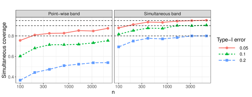
Figure 1 shows the simultaneous coverage of a confidence band generated by all point-wise confidence intervals (left) and the confidence band as specified in 6 at various values of $n$ and $\alpha$. We see that the latter method has coverage much closer to the nominal level than the former. Therefore, the point-wise procedure is insufficient for providing the correct simultaneous coverage, suggesting that the simultaneous adjustment is indeed necessary. This simulation also suggests that the coverage of the simultaneous band is not overly conservative.

Refer to caption
Figure 2: Coverage of CV risk confidence intervals for forward selection terminated at different values (left) and lasso at different regularization values (right). The dashed horizontal line marks the nominal level given by $1-\alpha$.

The importance of stability.

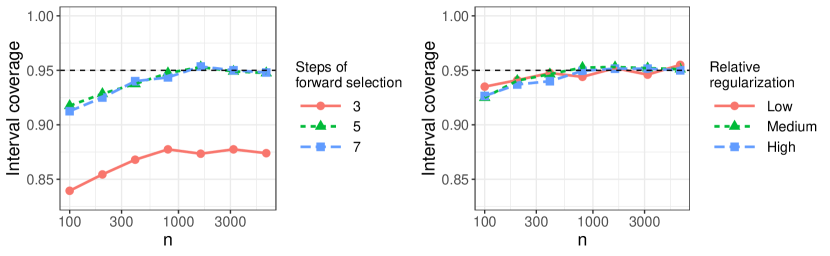
The impact of stability on the quality of Gaussian approximation of cross-validated risks has been experimented in Austern and Zhou (2020). Here we provide additional empirical results on this front. Consider confidence intervals for forward selection in the same setting but with $d=10$ and $\alpha=0.05$. Specifically, we look at the point-wise interval coverage of forward selection terminated at different model sizesโ€“one less than s๐‘ s, one equal to s๐‘ s, and one larger than s๐‘ s. The left plot in Figureย 2 shows that at 3 steps, the one-dimensional $95\%$-confidence interval based on Theoremย 3.1 under covers regardless of the sample size, while at 5 and 7 steps the coverage converges to nominal level as the sample size increases. This observation is consistent with the stability condition. Before s๐‘ s is reached, forward selection is quite unstable in this setting, as the non-zero entries of $\beta$ have the same magnitude. Therefore, the algorithm is equally likely to pick any subset of sโˆ’1๐‘ 1s-1 non-zero coordinates, and changing the value of one data point can incur a change of selected variables with non-negligible chance, resulting in instability of the loss function. When forward selection reaches exactly s๐‘ s steps, it selects the correct subset with overwhelming probability, leading to a stable loss function. When forward selection selects one more variable, the index of the additional selected variable is not stable but the fitted coefficient is very close to zero, so that the fitted loss function is still stable. In contrast, the lasso algorithm is continuous in the input data, hence the stability is much easier to hold for all values of penalty parameters, as suggested by the right plot in Figureย 2.

The advantage of difference-based model confidence sets.

Now we look at the model confidence set performance as applied to the lasso on data with increasing $n$. Specifically, we are studying the size $|\mathcal{A}|$ and coverage $\mathbb{P}(r^{*}\in{\mathcal{A}})$ for

  1. (1)

    the naรฏve method $\mathcal{A}=\hat{\mathcal{A}}_{0}$ as defined in (7), and

  2. (2)

    the difference based method $\mathcal{A}=\hat{\mathcal{A}}$ as defined in (8).

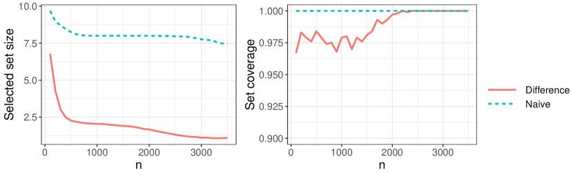
This simulation setting is again similar with the value of s๐‘ s fixed at 5, but $d$ grows at rate $n/10$. This time, to make our grid of regularization parameters, we first find $\lambda_{\text{max}}=\frac{1}{n}\|Z^{T}Y\|_{\infty}$, then the grid is defined by $\lambda_{\text{max}}2^{i}/\sqrt{1-1/V}$ for $i\in\{0,\dots,-9\}$. The re-scaling of $\sqrt{1-1/V}$ is done since the choice of $\lambda$ in lasso is inversely proportional to the square root of the training sample size, and $\lambda_{\max}$ may be a bit too small for the reduced sample size in $V$-fold cross-validation. The left plot of Figureย 3 shows that the difference based method produces considerably smaller sets while maintaining coverage of at least 0.95, supporting the intuition that the difference based method is able to take into account the joint randomness of the cross-validated risks. On the right plot of Figureย 3, the empirical coverage of the naรฏve method is always overly conservative, while the coverage of the difference based method does get closer to nominal level for certain values of $n$. Intuitively, such a fluctuation of coverage as $n$ varies can be explained by whether the problem is close to the boundary of the null hypothesis. More specifically, let ๐œนr=(R~rโˆ’R~s:sโ‰ r)\bm{\delta}_{r}=(\tilde{R}_{r}-\tilde{R}_{s}:s\neq r). In the difference based method, the null hypothesis for a candidate $r$ is that $\bm{\delta}_{r}$ is non-positive in each coordinate, which is a composite null hypothesis. The Gaussian approximation is derived precisely for the extreme point of the null hypothesis, where all coordinates of $\bm{\delta}_{r}$ are zero. In practice, we will never really be working in this scenario. Therefore, the supremum-based confidence set will be too conservative if $\bm{\delta}_{r}$ has many large negative coordinates, and will be nearly exact if most of the coordinates are close to 00. In our simulation, when $n$ increases, the relative performance of different tuning parameters also changes. Indeed we do observe that when $n\leq 2500$, the small sample size cannot quite distinguish the two best $\lambda$ values that perform nearly equally well.

Refer to caption
Figure 3: Size and coverage of model confidence set procedures with $\alpha=0.05$.

5 Stability condition examples

Before moving on to our Gaussian comparison results with deterministic centering, we pause to provide some context on the aforementioned stability conditions and discuss some settings wherein they are satisfied. Previously, the first order stability condition and its use in proving risk consistency of cross-validation were studied in Bousquet and Elisseeff (2002). In the study of low-dimensional CLTs for cross-validation, Austern and Zhou (2020) studied both first and second order stability conditions for parameters estimated as global minimums of convex optimization problems. In this section, we combine and extend these two lines of results. First, we prove the first and second order stability for stochastic gradient descent applied to convex and smooth objective functions. This result provides a more concrete example of stability by taking into consideration the particular optimization algorithm and its optimization error. We also believe our result has the correct technical conditions on the objective function for the second order, which is missing in Austern and Zhou (2020). Second, we provide an example in which the first and second order stability conditions hold for the difference loss function. This is a much more subtle task since the differences in loss functions often have vanishing variances.

5.1 Stability of stochastic gradient descent

Stochastic gradient descent (SGD) is one of the most popular optimization algorithms in large-scale machine learning. Thus stability of SGD is particularly important in our analysis of cross-validation. First order stability bounds for SGD were established in Hardt etย al. (2016) under convexity and smoothness assumptions, similar to those presented here and in Austern and Zhou (2020). Here, we will provide first and second order stability bounds for SGD.

Suppose the loss function $\ell:\mathcal{X}\rightarrow\mathbb{R}$ is written as $\ell(x)=\ell(x;\theta)$ and parameterized by $\theta\in\Theta$. A classical approach for estimating $\theta$ is to use an M-estimator,

$$\hat{\theta}=\operatorname*{arg\,min}_{\theta\in\Theta^{\prime}\subset\Theta}\sum_{i=1}^{n}\psi(\theta;X_{i}),$$ (9)

where $\psi:\Theta\rightarrow\mathbb{R}$ is an objective function, which may or may not be the same as $\ell$. A popular way to solve (9) is to use SGD, whereby we initialize $\hat{\theta}_{0}=0$ and then iteratively update

$$\hat{\theta}_{t+1}=\hat{\theta}_{t}-\alpha_{t+1}\dot{\psi}(\hat{\theta}_{t};X_{t+1})$$ (10)

for $t=1,\dots,n-1$ with step size $\alpha_{t}\geq 0$, where $\dot{\psi}(\theta;x)$ and $\ddot{\psi}(\theta;x)$ are the first and second partial derivatives of the objective function $\psi(\cdot,\cdot)$ with respect to $\theta$, respectively. Upon reaching $t=n-1$, we set $\hat{\theta}=\hat{\theta}_{n}$ which serves as our SGD estimator.

In order to obtain a first order stability bound for SGD, we consider the following smoothness and convexity assumptions of the objective function.

Assumption 3 (Smoothness and convexity of the objective function).

For all $x$,

  1. (a)

    $\psi(\cdot;x)$ is $\gamma$-strongly convex and L-Lipschitz

  2. (b)

    $\dot{\psi}(\cdot;x)$ is $\beta$-Lipschitz

These assumptions are standard in the learning-theoretic literature, and have been considered in Hardt etย al. (2016) to establish a similar first order stability result.

We now present our first order stability bound for SGD.

Proposition 5.1 (First order stability of SGD).

Under Assumptionย 3, if $\alpha_{t}=t^{-a}\beta^{-1}$ for some $a\in(0,1)$ and $\frac{\gamma}{\beta}\geq\frac{a(1-a)}{1-2^{-(1-a)}}\frac{\log n}{n^{1-a}}$, then

$$\left\|\nabla_{i}\hat{\theta}_{n}\right\|\leq\frac{2L}{\beta}n^{-a}$$

This proposition differs from the results in Hardt etย al. (2016) by considering a different decay speed of the step size. Also, Austern and Zhou (2020) used the same assumptions to establish the first order stability for the global optimum of M-estimators, but did not consider any optimization errors.

Before moving on to second order stability, we provide an example in which Assumptionย 3 is satisfied.

Example 3.

Consider ridge regression: $x=(y,z)\in\mathbb{B}(R_{x})$, and $\theta\in\mathbb{B}(R_{\theta})$, where $\mathbb{B}(R)$ denotes a centered Euclidean ball with radius $R$. Consider objective function

$$\psi(\theta;x)=\frac{1}{2}(y-z^{T}\theta)^{2}+\frac{1}{2}\lambda\|\theta\|^{2}\,.$$

Then $\psi$ is $\gamma$-strongly convex with $\gamma=\lambda$, $L$-Lipschitz with $L=R_{x}^{2}(1+R_{\theta})+\lambda R_{\theta}$, and $\beta$-smooth with $\beta=R_{x}^{2}+\lambda$.

The additional condition $\gamma/\beta\gg\frac{\log n}{n^{1-a}}$ can still hold if $R_{x}$, $R_{\theta}$, and $\lambda^{-1}$ vary as small polynomials of $n$.

Next, in order to provide a bound on the second order stability, we need to control the โ€œdifference in differenceโ€ of the loss functions, which inevitably involves the second order Taylor expansion and would require regularity of the Hessian of $\psi$.

Assumption 4 (Lipschitz Hessian).

For all $x$, $\ddot{\psi}(\cdot;x)$ is $L_{2}$-Lipschitz.

To the best of our knowledge, Assumptionย 4 has not appeared in the literature of stability of M-estimators. It is required to establish second order stability and we believe this condition is also needed for the second order stability proof in Austern and Zhou (2020).

Now we are ready to present our second order stability result for SGD.

Proposition 5.2 (Second order stability of SGD).

Under Assumptionย 4 and the same conditions as Propositionย 5.1,

$$\left\|\nabla_{j}\nabla_{i}\hat{\theta}_{n}\right\|\leq c(L,L_{2},a,\gamma,\beta)n^{-2a}\log n\,.$$

The constant $c(L,L_{a},a,\gamma,\beta)$ is explicitly tracked in the proof. The rate of $n^{-2a}$ is expected, while the additional $\log n$ factor arises in the proof when using a union bound on exponential tails.

For ridge regression, the additional requirement of Assumptionย 4 is trivial, as $\ddot{\psi}(\cdot;x)$ is constant. Here we consider a less trivial example.

Example 4.

Consider logistic ridge regression: $x=(y,z)\in\mathbb{B}(R_{x})$, and $\theta\in\mathbb{B}(R_{\theta})$.

$$\psi(\theta;z)=-yz^{T}\theta+\log(1+e^{z^{T}\theta})+\lambda\|\theta\|^{2}\,.$$

Then $\psi$ is $\gamma$-strongly convex with $\gamma=2\lambda$. $\psi$ is $L$-Lipschitz with $L=R_{x}^{2}+\frac{1}{R_{\theta}}\log(1+e^{R_{x}R_{\theta}})+\lambda R_{\theta}$, and $\beta$-smooth with $\beta=\frac{R_{x}}{R_{\theta}}+\lambda$. $\ddot{\psi}(\theta)$ is $L_{2}$-Lipschitz with $L_{2}=\frac{R_{x}^{2}}{4R_{\theta}}$.

The required $o(n^{-3/2})$ rate can be achieved when $a>3/4$ and $R_{x}$, $R_{\theta}$, $\lambda^{-1}$ grow slowly enough as $n$ increases.

From parameter stability to loss stability.

The first and second order stability for SGD established in Propositionsย 5.1 andย 5.2 are for the estimated parameter $\theta$. The corresponding stability conditions for the loss function $\ell(x;\theta)$ can be derived under suitable smoothness conditions on $\ell$. In particular, if we assume that for each $x$, both $\ell(x;\theta)$ and $\dot{\ell}(x;\theta)$ are Lipschitz, then, using a standard first order Taylor expansion of $\ell(x;\theta)$ with respect to $\theta$, we have

$\displaystyle\left|\nabla_{i}\ell(x;\hat{\theta}_{n})\right|\leq C_{1}\left\|\nabla_{i}\hat{\theta}_{n}\right\|\,,~{}~{}~{}~{}\left|\nabla_{j}\nabla_{i}\ell(x;\hat{\theta}_{n})\right|\leq C_{2}\left(\left\|\nabla_{j}\nabla_{i}\hat{\theta}_{n}\right\|+\sup_{i}\left\|\nabla_{i}\hat{\theta}_{n}\right\|^{2}\right)\,,$

where $C_{1}$ is a constant depends on the Lipschitz constant of $\ell(x;\cdot)$, and $C_{2}$ is a constant depends on the Lipschitz constants of $\ell(x;\cdot)$ and $\dot{\ell}(x;\cdot)$. As a result, when $a$ is large enough and the Lipschitz constants in $\psi(x;\cdot)$, $\ell(x;\cdot)$ and their derivatives do not grow too fast, the first and second order loss stability conditions can be satisfied.

5.2 Stability of difference loss: a nonparametric regression example

Establishing the stability conditions for difference losses as required in Propositionย 4.2 is more delicate, mainly because Assumptionย 2(c) will be violated. For the Gaussian comparison argument to work, one needs to re-standardize the loss functions by considering

โˆ‡i(โ„“rโˆ’โ„“s)Varโ€‹(โ„“rโˆ’โ„“s)andโˆ‡jโˆ‡i(โ„“rโˆ’โ„“s)Varโ€‹(โ„“rโˆ’โ„“s)subscriptโˆ‡๐‘–subscriptโ„“๐‘Ÿsubscriptโ„“๐‘ Varsubscriptโ„“๐‘Ÿsubscriptโ„“๐‘ andsubscriptโˆ‡๐‘—subscriptโˆ‡๐‘–subscriptโ„“๐‘Ÿsubscriptโ„“๐‘ Varsubscriptโ„“๐‘Ÿsubscriptโ„“๐‘ \frac{\nabla_{i}(\ell_{r}-\ell_{s})}{\sqrt{{\rm Var}(\ell_{r}-\ell_{s})}}~{}~{}~{}~{}\text{and}~{}~{}~{}~{}\frac{\nabla_{j}\nabla_{i}(\ell_{r}-\ell_{s})}{\sqrt{{\rm Var}(\ell_{r}-\ell_{s})}}

in Assumptionย 2(a) and 2(b), respectively. In general, the variance of โ„“rโˆ’โ„“ssubscriptโ„“๐‘Ÿsubscriptโ„“๐‘ \ell_{r}-\ell_{s} depends on the bias-variance decomposition of the two models, which may cancel with each other at different rates. A general treatment of such a variance of difference loss functions seems to be a challenging task, if at all possible, and we will not pursue this in the current paper. Instead, we use a simple non-parametric example to explicitly quantify the variance and stability of difference loss functions.

In particular, consider the following linear regression model with an infinite dimensional feature vector. Let $(X_{i}:1\leq i\leq n)$ be iid vectors with $X_{i}=(Y_{i},Z_{i})\in\mathbb{R}^{1}\times\mathbb{R}^{\infty}$, such that

$$Y_{i}=\sum_{j=1}^{\infty}\beta_{j}Z_{ij}+\epsilon_{i}$$ (11)

where

  1. 1.

    $\epsilon_{i}$ is independent of $Z_{i}$, has mean zero, finite variance $\sigma_{\epsilon}^{2}$, and is $1$-SW;

  2. 2.

    $Z_{ij}$ is mean zero, has unit variance, is $1$-SW, and satisfies $\mathbb{E}(Z_{ij}|Z_{i1},...,Z_{i,j-1})=0$ for all $j$;

  3. 3.

    $\beta_{j}\asymp j^{-\frac{1+a}{2}}$ for some $a>0$ for all $j$โ€‰.

The zero mean and unit variance will simplify the estimator. The sub-Weibull conditions will be carried over to the difference of the loss functions. The rate of $\beta_{j}$ allows us to track the bias and variance precisely.

For each $j$, we can naturally estimate $\beta_{j}$ by

$$\hat{\beta}_{j}=\frac{1}{n}\sum_{i=1}^{n}Y_{i}Z_{ij}\,.$$

For each candidate model $r$, let $J_{r}=J_{r,n}$ be a positive integer such that $J_{n,r}\rightarrow\infty$ at a speed that is specified by the model $r$. For example $J_{r,n}=n^{\alpha_{r}}$, where $\{\alpha_{r}:r\in\mathcal{M}\}$ is a collection of positive numbers corresponding to different increase speed of $J_{r,n}$. The estimates we consider are truncated sequence estimates defined by integers $J_{r}$,

$\displaystyle\hat{f}_{r}(Z_{0})=\sum_{j=1}^{J_{r}}\hat{\beta}_{j}Z_{0j}\,,~{}~{}\forall~{}~{}r\in\mathcal{M}\,.$
Proposition 5.3 (Loss difference stability in the nonparametric regression example).

Under the regression model (11) and the conditions for $\epsilon$, $Z$, $\beta$, if Jrโ‰คcโ€‹Jssubscript๐ฝ๐‘Ÿ๐‘subscript๐ฝ๐‘ J_{r}\leq cJ_{s} for some constant $c\in(0,1)$, then

  • (a)

    the first order stability required in Propositionย 4.2 holds when Jsโ€‹Jra/2=oโ€‹(n)subscript๐ฝ๐‘ superscriptsubscript๐ฝ๐‘Ÿ๐‘Ž2๐‘œ๐‘›J_{s}J_{r}^{a/2}=o(n);

  • (b)

    the second order stability required in Propositionย 4.2 holds when Jsโ€‹Jra/2=oโ€‹(n)subscript๐ฝ๐‘ superscriptsubscript๐ฝ๐‘Ÿ๐‘Ž2๐‘œ๐‘›J_{s}J_{r}^{a/2}=o(\sqrt{n}).

Remark 5.

Under the specified decay speed $\beta_{j}\asymp j^{-1-a}$, the optimal truncation $J^{*}$ that minimizes the risk under the squared prediction loss is $J^{*}\asymp n^{\frac{1}{1+a}}$. If Jsโ‰ซJrโ‰Jโˆ—much-greater-thansubscript๐ฝ๐‘ subscript๐ฝ๐‘Ÿasymptotically-equalssuperscript๐ฝJ_{s}\gg J_{r}\asymp J^{*}, the the condition Jsโ€‹Jra/2=oโ€‹(n)subscript๐ฝ๐‘ superscriptsubscript๐ฝ๐‘Ÿ๐‘Ž2๐‘œ๐‘›J_{s}J_{r}^{a/2}=o(\sqrt{n}) cannot be satisfied. This implies the stability condition is harder to satisfy if the estimate from model s๐‘ s has large variance. On the other hand, if Jโˆ—โ‰Jsasymptotically-equalssuperscript๐ฝsubscript๐ฝ๐‘ J^{*}\asymp J_{s}, then the condition Jsโ€‹Jra/2=oโ€‹(n)subscript๐ฝ๐‘ superscriptsubscript๐ฝ๐‘Ÿ๐‘Ž2๐‘œ๐‘›J_{s}J_{r}^{a/2}=o(\sqrt{n}) can be satisfied when $a>1$ and $J_{r}\lesssim n^{(a-1)/(a+a^{2})}$. Again, this agrees with the intuition that cross-validation is able to screen out inferior models that have large bias Yang (2007).

6 On deterministic centering

So far, we have focused on the high dimensional Gaussian comparison of cross-validated risk with random centering, where the mean vector $\tilde{\mathbf{R}}$ is data-dependent. This leads to the following question: can we establish Gaussian comparison results with fixed centering? It is natural to expect the fixed centering to be $\mathbf{R}^{*}=\mathbb{E}(\hat{\mathbf{R}}_{\rm cv})$. Also, the corresponding scaling should be based on the total variance $\mathbb{E}\left[\bm{\ell}(X_{0};\mathbf{X}_{-1})\bm{\ell}(X_{0};\mathbf{X}_{-1})^{T}\right]-\mathbf{R}^{*}{{\mathbf{R}}^{*}}^{T}$, which in addition to the variance term $\Sigma$ considered in the random centering case above, must also take into account the variability caused by the randomness of $\mathbf{R}(\mathbf{X}_{-1})$. Such a fixed centering central limit theorem for cross-validated risks has been studied in Austern and Zhou (2020) in the low-dimensional case. Our development here extends their result to the high-dimensional case with a more streamlined proof.

6.1 Risk stability

In order to study the randomness in the risk function $R_{r}(\mathbf{X}_{-1})$, we need the following stability conditions on the risk functions.

Assumption 5 (Risk stability).

There exists a constant $\epsilon_{R}\in\mathbb{R}^{+}$ such that $n\nabla_{i}R_{r}(\mathbf{X}_{-1})$ is $\epsilon_{R}$-SW for all $i$.

A remarkable difference between the risk stability and loss stability is in the scaling factors. For the first order differencing operators $\nabla_{i}$, the scaling factor of $n$ instead of $\sqrt{n}$ makes the risk stability apparently harder to control than the loss stability. This is also considered and briefly discussed in Austern and Zhou (2020) in the low-dimensional case. Here, we give a detailed explanation of this key condition. At first, it seems unreasonable to assume that $\epsilon_{R}$ is very small, as $\nabla_{i}R_{r}(\mathbf{X}_{-1})$ generally should not be smaller than $1/n$. However, a closer inspection suggests that the risk function (taking expectation of the loss function $\ell_{r}(X_{0},\mathbf{X}_{-1})$ over the evaluating point $X_{0}$) is usually much more stable than the loss function itself, as taking a conditional expectation usually increases stability. In fact, such an increase of stability can be quite substantial. For example, assume that the loss function takes a parametric form: $\ell(x_{0};x_{1},...,x_{\tilde{n}})=\ell(x_{0};\hat{\theta})$ where $\hat{\theta}=\hat{\theta}(x_{1},...,x_{\tilde{n}})$ is a fitted parameter from the input data $(x_{1},...,x_{\tilde{n}})$. Then

$$\nabla_{i}R(\hat{\theta})\approx\left(\frac{dR}{d\theta}\bigg{|}_{\hat{\theta}}\right)\nabla_{i}\hat{\theta}\,,$$

which should be much smaller than $\nabla_{i}\hat{\theta}$ if $R(\theta)\coloneqq\mathbb{E}\ell(X_{0};\theta)$ is flat at $\hat{\theta}$. This is usually the case when $\hat{\theta}$ is in a small neighborhood of the optimal parameter value with minimum risk $\theta^{*}$.

Furthermore, we remark that our theoretical development does not require $\epsilon_{R}$ to vanish asymptotically. Instead, we only need $\epsilon_{R}$ to be dominated by other vanishing terms such as $\epsilon_{\ell}$ and $1/\sqrt{n}$.

6.2 Gaussian comparison with deterministic centering

Finding the covariance matrix for deterministic centering starts by identifying the contribution of randomness from each single sample point. We start by writing

$$n\hat{R}_{{\rm cv},r}=\sum_{i=1}^{n}\ell_{r}(X_{i};\mathbf{X}_{-v_{i}})\,.$$

The part in the above sum that involves $X_{i}$ is

$\displaystyle\ell_{r}(X_{i};\mathbf{X}_{-v_{i}})+\sum_{j\notin I_{v_{i}}}\ell_{r}(X_{j};\mathbf{X}_{-v_{j}})\,.$ (12)

It is clear that $X_{i}$ plays two different roles in $\hat{R}_{{\rm cv},r}$: (i) as the evaluation point in $\ell_{r}(X_{i};\mathbf{X}_{-v_{i}})$, (ii) as one of the $\tilde{n}$ fitting sample points in each of $\ell_{r}(X_{j};\mathbf{X}_{-v_{j}})$ for jโ‰ Ivi๐‘—subscript๐ผsubscript๐‘ฃ๐‘–j\neq I_{v_{i}}. The randomness contributed by $X_{i}$ as an evaluating point should be captured by the variability of the average loss function

$$\bar{\ell}_{r}(X_{1})=\mathbb{E}\left[\ell_{r}(X_{1};\mathbf{X}_{-1})|X_{1}\right]\,,$$

and the randomness contributed by $X_{1}$ as a fitting sample point should be captured in the function

$$\bar{R}_{r}(X_{1})=\mathbb{E}\left[R(\mathbf{X}_{-V})|X_{1}\right]\,.$$

Therefore, let $\bm{\Phi}=(\phi_{rs}:1\leq r,s\leq p)$ be the covariance matrix given by

ฯ•rโ€‹sโ‰”โ‰”subscriptitalic-ฯ•๐‘Ÿ๐‘ absent\displaystyle\phi_{rs}\coloneqq Covโ€‹[โ„“ยฏrโ€‹(X1)+n~โ€‹Rยฏrโ€‹(X1),โ„“ยฏsโ€‹(X1)+n~โ€‹Rยฏsโ€‹(X1)]โ€‹1โ‰คr,sโ‰คp.formulae-sequenceCovsubscriptยฏโ„“๐‘Ÿsubscript๐‘‹1~๐‘›subscriptยฏ๐‘…๐‘Ÿsubscript๐‘‹1subscriptยฏโ„“๐‘ subscript๐‘‹1~๐‘›subscriptยฏ๐‘…๐‘ subscript๐‘‹11๐‘Ÿ๐‘ ๐‘\displaystyle{\rm Cov}\left[\bar{\ell}_{r}(X_{1})+\tilde{n}\bar{R}_{r}(X_{1})\,,~{}\bar{\ell}_{s}(X_{1})+\tilde{n}\bar{R}_{s}(X_{1})\right]\,~{}~{}1\leq r,s\leq p\,. (13)

We assume that the marginal variance terms are bounded and bounded away from 00, leading to the following assumption which is analogous to Assumptionย 1(b).

Assumption 6.

There exist positive constants $\underline{\phi}$ and $\bar{\phi}$ such that $\underline{\phi}\leq\phi_{rr}\leq\bar{\phi}$ for each $r\in[p]$.

Using this assumption on the marginal variance terms, the symmetry and moment condition on $\ell_{r}$, and all previous stability assumptions on $\ell_{r}$ and $R_{r}$, we state the following result for the Gaussian comparison with fixed centering.

Theorem 6.1 (Deterministic Gaussian Comparison).

Assume Assumptionsย 1, 2, 5 andย 6 hold, then we have

$\displaystyle\sup_{z\in\mathbb{R}}\left|\mathbb{P}\left(\sqrt{n}\max(\hat{\mathbf{R}}_{\rm cv}-\mathbf{R}^{*})\leq z\right)-\mathbb{P}\left(\max\mathbf{Y}\leq z\right)\right|$
$\displaystyle\leq\tilde{O}\left([\epsilon_{\ell}(1+\epsilon_{R})]^{1/3}+n^{-1/8}(1+\epsilon_{R})^{3/4}\right)$

for $\mathbf{Y}\sim N(0,\bm{\Phi})$.

Remark 6.

Similar to Remarkย 3, the constants $\bar{\phi}$ and $\underline{\phi}$ appear in the error bound as a multiplicative factor in the $\tilde{O}(\cdot)$ notation, which is no larger than $\bar{\phi}\underline{\phi}^{-2}$.

6.3 Deterministic variance estimation

Finally, we address the problem of estimating ฯ•rโ€‹ssubscriptitalic-ฯ•๐‘Ÿ๐‘ \phi_{rs}, which has also been considered in Austern and Zhou (2020). We believe the estimate stated in their text is off by a factor of 2, and also only covers the case of two-fold cross-validation. Our result below corrects the scaling and covers the general $V$-fold case in a multivariate setting.

As suggested in (13) and Theoremย 6.1, the covariance ฯ•rโ€‹ssubscriptitalic-ฯ•๐‘Ÿ๐‘ \phi_{rs} is essentially the sum of the marginal variability of each $X_{i}$. Indeed, we have the following result

Theorem 6.2 (Marginal variance approximation).

Under Assumptionsย 1, 2, 5 andย 6, we conclude that

n22โ€‹๐”ผโ€‹[โˆ‡iR^cv,rโ€‹โˆ‡iR^cv,s|๐—โˆ’vi]โˆ’ฯ•rโ€‹ssuperscript๐‘›22๐”ผdelimited-[]conditionalsubscriptโˆ‡๐‘–subscript^๐‘…cv๐‘Ÿsubscriptโˆ‡๐‘–subscript^๐‘…cv๐‘ subscript๐—subscript๐‘ฃ๐‘–subscriptitalic-ฯ•๐‘Ÿ๐‘ \frac{n^{2}}{2}\mathbb{E}\left[\nabla_{i}\hat{R}_{{\rm cv},r}\nabla_{i}\hat{R}_{{\rm cv},s}|\mathbf{X}_{-v_{i}}\right]-\phi_{rs}

is $\epsilon_{\ell}(1+\epsilon_{R})$-SW.

Theoremย 6.2 implies that we can simply estimate ๐”ผโ€‹[โˆ‡1R^cv,rโ€‹โˆ‡1R^cv,s|๐—v1]๐”ผdelimited-[]conditionalsubscriptโˆ‡1subscript^๐‘…cv๐‘Ÿsubscriptโˆ‡1subscript^๐‘…cv๐‘ subscript๐—subscript๐‘ฃ1\mathbb{E}[\nabla_{1}\hat{R}_{{\rm cv},r}\nabla_{1}\hat{R}_{{\rm cv},s}|\mathbf{X}_{v_{1}}] to approximate ฯ•rโ€‹ssubscriptitalic-ฯ•๐‘Ÿ๐‘ \phi_{rs}. This leads to the following procedure, which requires a hold-out set of iid sample points $X_{1}^{\prime},...,X_{m}^{\prime}$ from the same distribution, that are not involved in any cross-validation folds. In practice, one can choose a small but diverging value of $m=n^{a}$ with $a\in(0,1)$, then use $n-m$ sample points for the $V$-fold cross-validation and $m$ hold-out sample points for variance estimation.

For $i\in[n]$ and $j\in[m]$, define $\hat{\mathbf{R}}_{{\rm cv}}^{i,j}$ to be the cross-validation risk vector obtained by replacing $X_{i}$ with $X_{j}^{\prime}$. Then Theoremย 6.2 implies the following.

Corollary 6.3.

Define

ฯ•^rโ€‹s=n2mโ€‹โˆ‘j=1m/2(R^cv,r1,2โ€‹jโˆ’1โˆ’R^cv,r1,2โ€‹j)โ€‹(R^cv,s1,2โ€‹jโˆ’1โˆ’R^cv,s2โ€‹j).subscript^italic-ฯ•๐‘Ÿ๐‘ superscript๐‘›2๐‘šsuperscriptsubscript๐‘—1๐‘š2superscriptsubscript^๐‘…cv๐‘Ÿ12๐‘—1superscriptsubscript^๐‘…cv๐‘Ÿ12๐‘—superscriptsubscript^๐‘…cv๐‘ 12๐‘—1superscriptsubscript^๐‘…cv๐‘ 2๐‘—\displaystyle\hat{\phi}_{rs}=\frac{n^{2}}{m}\sum_{j=1}^{m/2}\left(\hat{R}_{{\rm cv},r}^{1,2j-1}-\hat{R}_{{\rm cv},r}^{1,2j}\right)\left(\hat{R}_{{\rm cv},s}^{1,2j-1}-\hat{R}_{{\rm cv},s}^{2j}\right)\,. (14)

Then with probability at least $1-O((n+p)^{-1})$ we have

supr,s|ฯ•^rโ€‹sโˆ’ฯ•rโ€‹s|โ‰คO~โ€‹(ฯตโ„“โ€‹(1+ฯตR)+mโˆ’1/2).subscriptsupremum๐‘Ÿ๐‘ subscript^italic-ฯ•๐‘Ÿ๐‘ subscriptitalic-ฯ•๐‘Ÿ๐‘ ~๐‘‚subscriptitalic-ฯตโ„“1subscriptitalic-ฯต๐‘…superscript๐‘š12\sup_{r,s}|\hat{\phi}_{rs}-\phi_{rs}|\leq\tilde{O}\left(\epsilon_{\ell}(1+\epsilon_{R})+m^{-1/2}\right)\,.

The estimator in (14) estimates ๐”ผโ€‹[โˆ‡1R^cv,rโ€‹โˆ‡1R^cv,s|๐—โˆ’v1]๐”ผdelimited-[]conditionalsubscriptโˆ‡1subscript^๐‘…cv๐‘Ÿsubscriptโˆ‡1subscript^๐‘…cv๐‘ subscript๐—subscript๐‘ฃ1\mathbb{E}[\nabla_{1}\hat{R}_{{\rm cv},r}\nabla_{1}\hat{R}_{{\rm cv},s}|\mathbf{X}_{-v_{1}}] by taking empirical average over $m/2$ conditional iid samples given the fitting data $\mathbf{X}_{-v_{1}}$, which is supported by Lemmaย D.1 and Lemmaย D.2. In practice, we can possibly also use

ฯ•^rโ€‹s=n22โ€‹mโ€‹โˆ‘j=1m(R^cv,rโˆ’R^cv,rij,j)โ€‹(R^cv,sโˆ’R^cv,sij,j).subscript^italic-ฯ•๐‘Ÿ๐‘ superscript๐‘›22๐‘šsuperscriptsubscript๐‘—1๐‘šsubscript^๐‘…cv๐‘Ÿsuperscriptsubscript^๐‘…cv๐‘Ÿsubscript๐‘–๐‘—๐‘—subscript^๐‘…cv๐‘ superscriptsubscript^๐‘…cv๐‘ subscript๐‘–๐‘—๐‘—\hat{\phi}_{rs}=\frac{n^{2}}{2m}\sum_{j=1}^{m}\left(\hat{R}_{{\rm cv},r}-\hat{R}_{{\rm cv},r}^{i_{j},j}\right)\left(\hat{R}_{{\rm cv},s}-\hat{R}_{{\rm cv},s}^{i_{j},j}\right)\,.

which perturbs different entries instead of just the first one.

Corollaryย 6.3 provides an entry-wise error bound of the covariance estimation, which is good enough for Gaussian approximation of the supremum, as demonstrated in Corollaryย 4.1. The same kind of inference procedures considered in Sectionย 4 can be carried over to the deterministic centering case, which is omitted here as there is little additional insight.

7 Discussion

Since its first appearance, high-dimensional Gaussian comparisons have found wide applications in statistical inference problems, and have been extended and improved by many authors. In addition to the extensions to dependent data mentioned above, sharper results on the Gaussian comparison of independent sums have been obtained in recent literature. For example, see Deng and Zhang (2020); Kuchibhotla etย al. (2021); Lopes (2020); Kuchibhotla and Rinaldo (2020). In our work, the goal is to develop an asymptotic Gaussian comparison to serve the purpose of statistical inference. Thus we did not attempt to obtain the optimal Berry-Esseen type of convergence rates. Our proof uses the Slepian interpolation as in the original work Chernozhukov etย al. (2013), and it seems possible to obtain better rates of convergence if more refined techniques are used.

Our main motivations are to understand the joint randomness of many cross-validated risks, and to provide theoretical foundations for uncertainty quantification of cross-validation based model selection. The theory included in this work is particularly relevant to the โ€œcross-validation with confidenceโ€ method (Lei, 2020), where one uses the asymptotic Gaussian comparison to construct a confidence set that contains the best model with a prescribed confidence level. This method is connected to the model selection confidence set literature (Hansen etย al., 2011), which has largely relied on sequential hypothesis testing based approaches (Gunes and Bondell, 2012; Ferrari and Yang, 2015; Jiang etย al., 2008). We expect the theory outlined in this paper to be useful in developing a new model confidence set estimator using cross-validation with both provable validity guarantees and good practical performance.

Appendix A More notation, definition, and basic properties

A.1 Definition and properties of sub-Weibull concentration

Definition 2 (sub-Weibull).

Let $K,\alpha$ be positive numbers. We say a random variable $X$ is $(K,\alpha)$-sub-Weibull (or $(K,\alpha)$-SW) if any of the following holds:

  1. 1.

    There exists constant $a$ such that $\mathbb{P}\left(\frac{|X|}{K}\geq t\right)\leq ae^{-t^{\alpha}}$, for all $t>0$.

  2. 2.

    There exists constant $c$ such that $\|X\|_{q}\leq cKq^{1/\alpha}$ for all $q\geq 1$.

The equivalence of these two definitions can be found in, for example, Theorem 2.1 of Vladimirova etย al. (2020). The constants $a,c$ in the definition above are not important, and are used here so that the two definitions have the same $(K,\alpha)$ pair.

Proposition A.1 (Basic properties of sub-Weibull random variables).

If $X_{i}$ is $(K_{i},\alpha_{i})$-SW, for $i=1,2$, then

  1. 1.

    $X_{1}X_{2}$ is $(K_{1}K_{2},\frac{\alpha_{1}\alpha_{2}}{\alpha_{1}+\alpha_{2}})$-SW.

  2. 2.

    $X_{1}+X_{2}$ is $(K_{1}\vee K_{2},\alpha_{1}\wedge\alpha_{2})$-SW.

The following theorem controls the tail integral of sub-Weibull random variables.

Lemma A.2.

If $Y$ is $(K,\alpha)$-sub-Weibull, then there exists constant $c>0$ independent of $K$ such that $\mathbb{E}[|Y|\mathds{1}(|Y|\geq wK)]\leq cKw\exp(-w^{\alpha})$ for any $w\geq 1$.

Proof of Lemmaย A.2.

Without loss of generality, assume $Y\geq 0$ and $K=1$. Let $f(y)$ be the density function of $Y$.

$\displaystyle\mathbb{E}[Y\mathds{1}(Y\geq w)]=$ $\displaystyle\int_{y=w}^{\infty}yf(y)dy$
$\displaystyle=$ $\displaystyle\int_{y=w}^{\infty}\int_{u=0}^{y}duf(y)dy$
$\displaystyle=$ $\displaystyle\int_{u=0}^{w}\int_{y=w}^{\infty}f(y)dydu+\int_{u=w}^{\infty}\int_{y=u}^{\infty}f(y)dydu$
$\displaystyle=$ $\displaystyle w\mathbb{P}(Y\geq w)+\int_{u=w}^{\infty}\mathbb{P}(Y\geq u)du$
$\displaystyle\leq$ $\displaystyle wa\exp(-w^{\alpha})+\int_{u=w}^{\infty}a\exp(-u^{\alpha})du$
$\displaystyle=$ $\displaystyle wa\exp(-w^{\alpha})+\frac{a}{\alpha}\int_{v=w^{\alpha}}^{\infty}\exp(-v)v^{\frac{1}{\alpha}-1}dv\,.$

When $\alpha\in(0,1]$, since $w\geq 1$ we have, by (Gabcke, 1979, Proposition 4.4.3)

$\displaystyle\int_{v=w^{\alpha}}^{\infty}\exp(-v)v^{\frac{1}{\alpha}-1}dv\leq\frac{1}{\alpha}e^{-w^{\alpha}}w^{1-1/\alpha}\,.$

Thus, $\mathbb{E}[Y\mathds{1}(Y\geq w)]\leq a(1+\alpha^{-2})w\exp(-w^{\alpha})$.

When $\alpha>1$, $v^{1/\alpha-1}\leq 1$ on $[w,\infty)$ since $w\geq 1$, so we have

$\displaystyle\int_{v=w^{\alpha}}^{\infty}\exp(-v)v^{\frac{1}{\alpha}-1}dv\leq\exp(-w^{\alpha})\,.$

So $\mathbb{E}[Y\mathds{1}(Y\geq w)]\leq 2aw\exp(-w^{\alpha})$โ€‰. โˆŽ

The following lemma is a sub-Weibull version of martingale concentration inequality, showing that the scaling of a martingale with stationary sub-Weibull increments scales at the speed of $\sqrt{n}$, where $n$ is the time horizon.

Lemma A.3.

Let $M=\sum_{i=1}^{n}M_{i}$ where the sequence $(M_{i})_{i=1}^{n}$ satisfies

  1. 1.

    martingale property: $\mathbb{E}(M_{i}|M_{j}:1\leq j<i)=0$ for all $2\leq i\leq n$, and $\mathbb{E}M_{1}=0$.

  2. 2.

    sub-Weibull tail: $\|M_{i}\|_{q}\leq cK_{i}q^{1/\alpha_{i}}$ for some $c,\alpha_{i}>0$ and all $q\geq 1$.

Then we have, for $\alpha^{\prime}=\frac{2\alpha^{*}}{2+\alpha^{*}}$ with $\alpha^{*}=\min_{j\leq n}\alpha_{j}$ and a positive constant $c^{\prime}$,

$$\|M\|_{q}\leq c^{\prime}\left(\sum_{i=1}^{n}K_{i}^{2}\right)^{1/2}q^{1/\alpha^{\prime}}\,,~{}~{}\forall q\geq 1\,.$$

If $K_{i}=K$ for all $i\in[n]$, then

$$\|M\|_{q}\leq c^{\prime}\sqrt{n}Kq^{1/\alpha^{\prime}}\,,~{}~{}\forall q\geq 1\,.$$
Proof of Lemmaย A.3.

By Theorem 2.1 of Rio (2009), we have for any $q\geq 2$

$\displaystyle\left\|M\right\|_{q}\leq\left[(q-1)\sum_{i=1}^{n}\|M_{i}\|_{q}^{2}\right]^{1/2}\leq\left[C(q-1)q^{2/\alpha^{*}}\sum_{i=1}^{n}K_{i}^{2}\right]^{1/2}\leq C^{1/2}q^{\frac{2+\alpha^{*}}{2\alpha^{*}}}\left(\sum_{i=1}^{n}K_{i}^{2}\right)^{1/2}\,.$

where $C$ is a constant depending only on $c$, and the second inequality follows from the assumption $\|M_{i}\|_{q}\leq cK_{i}q^{1/\alpha_{i}}$. โˆŽ

Appendix B Proof for random centering

B.1 Notation

We first collect some notation for the proof. For the ease of presentation, we use $\mathbf{W}=(W_{r}:1\leq r\leq p)$ to denote the centered and scaled random vector for which we would like to establish a normal approximation. Thus, in the proof that follows, the symbol $W_{r}$ may refer to different objects than in other proofs in this work. In particular, for the random centering/scaling case (Theoremย 3.1), $W_{r}=\sqrt{n}(\hat{R}_{{\rm cv},r}-\tilde{R}_{r})$, while in the deterministic centering/scaling case (Theoremย 6.1), $W_{r}=\sqrt{n}(\hat{R}_{{\rm cv},r}-R_{r}^{*}).$

Recall the following notation:

  • โ€ข

    ๐—โˆ’vsubscript๐—๐‘ฃ\mathbf{X}_{-v}: the $\tilde{n}$ ($=n(1-1/V)$) subvector of $\mathbf{X}$ excluding those in index $I_{v}$.

  • โ€ข

    ๐—โˆ’isuperscript๐—๐‘–\mathbf{X}^{-i}: the $(n-1)$ subvector of $\mathbf{X}$ excluding the $i$th entry.

  • โ€ข

    ๐—isuperscript๐—๐‘–\mathbf{X}^{i}: the iid vector of $\mathbf{X}$ with $i$th entry being $X_{i}^{\prime}$, an iid copy of $X_{i}$.

For random objects $(U,V)$ and function $f$ acting on $(U,V)$, we will also use the notation $\mathbb{E}_{U}f(U,V)=\mathbb{E}[f(U,V)|V]$. For example $\mathbb{E}_{X_{i}}f(\mathbf{X})=\mathbb{E}[f(\mathbf{X})|\mathbf{X}^{-i}]$.

B.2 Proof of Theoremย 3.1

Proof of Theoremย 3.1.

Recall the notation:

$$W_{r}=\sqrt{n}(\hat{R}_{{\rm cv},r}-\tilde{R}_{r})=\sum_{i=1}^{n}\frac{1}{\sqrt{n}}K_{r,i}\,.$$

Consider the leave-one-out version of $W_{r}$:

Wri=โˆ‘jโ‰ iKjโ€‹(๐—i)/n=Wrโˆ’1nโ€‹Kr,iโˆ’1nโ€‹Dr,i.superscriptsubscript๐‘Š๐‘Ÿ๐‘–subscript๐‘—๐‘–subscript๐พ๐‘—superscript๐—๐‘–๐‘›subscript๐‘Š๐‘Ÿ1๐‘›subscript๐พ๐‘Ÿ๐‘–1๐‘›subscript๐ท๐‘Ÿ๐‘–W_{r}^{i}=\sum_{j\neq i}K_{j}(\mathbf{X}^{i})/\sqrt{n}=W_{r}-\frac{1}{\sqrt{n}}K_{r,i}-\frac{1}{\sqrt{n}}D_{r,i}\,.

The plan is to use Slepianโ€™s interpolation which smoothly bridges between $\mathbf{W}$ and the corresponding Gaussian vector $\mathbf{Y}$. In order to do so, we consider an intermediate object

$$\hat{\mathbf{Y}}=\frac{1}{\sqrt{n}}\sum_{i=1}^{n}\hat{\mathbf{Y}}_{i}\coloneqq\frac{1}{\sqrt{n}}\sum_{i=1}^{n}\Sigma_{v_{i}}^{1/2}\varepsilon_{i}$$

with $\varepsilon_{i}\stackrel{{\scriptstyle iid}}{{\sim}}N(0,I_{p})$, ฮฃv=[ฯƒrโ€‹s,v]1โ‰คr,sโ‰คpsubscriptฮฃ๐‘ฃsubscriptdelimited-[]subscript๐œŽ๐‘Ÿ๐‘ ๐‘ฃformulae-sequence1๐‘Ÿ๐‘ ๐‘\Sigma_{v}=[\sigma_{rs,v}]_{1\leq r,s\leq p} being the conditional covariance matrix of $\mathbf{K}(X_{0};\mathbf{X}_{-v})$ given the fitting data $\mathbf{X}_{-v}$, and $v_{i}$ the fold identifier of the sample point indexed by $i$.

Define the interpolating vector, for $t\in(0,1)$

$$Z_{r}(t)=\sqrt{t}W_{r}+\sqrt{1-t}\sum_{i}\hat{Y}_{r,i}/\sqrt{n}\,,$$

and the corresponding leave-one-out version

Zriโ€‹(t)=tโ€‹Wri+1โˆ’tโ€‹โˆ‘jโ‰ iY^r,i/nsuperscriptsubscript๐‘๐‘Ÿ๐‘–๐‘ก๐‘กsuperscriptsubscript๐‘Š๐‘Ÿ๐‘–1๐‘กsubscript๐‘—๐‘–subscript^๐‘Œ๐‘Ÿ๐‘–๐‘›\displaystyle Z_{r}^{i}(t)=\sqrt{t}W_{r}^{i}+\sqrt{1-t}\sum_{j\neq i}\hat{Y}_{r,i}/\sqrt{n}

which satsifies

$$Z_{r}(t)-Z_{r}^{i}(t)=Z_{r,i}(t)+D_{i}(t)$$

with

$\displaystyle Z_{r,i}(t)=$ $\displaystyle\sqrt{t}K_{i}/\sqrt{n}+\sqrt{1-t}\hat{Y}_{r,i}/\sqrt{n}\,,$
$\displaystyle D_{r,i}(t)=$ $\displaystyle\sqrt{t}D_{r,i}/\sqrt{n}\,.$

Let $h:\mathbb{R}^{p}\mapsto\mathbb{R}$ be such that for all $z\in\mathbb{R}$. Define

โˆ‘r,s=1p|โˆ‚rโˆ‚shโ€‹(z)|=superscriptsubscript๐‘Ÿ๐‘ 1๐‘subscript๐‘Ÿsubscript๐‘ โ„Ž๐‘งabsent\displaystyle\sum_{r,s=1}^{p}|\partial_{r}\partial_{s}h(z)|= $\displaystyle M_{2}(h)\,,$ (15)
โˆ‘r,s,u=1p|โˆ‚rโˆ‚sโˆ‚uhโ€‹(z)|=superscriptsubscript๐‘Ÿ๐‘ ๐‘ข1๐‘subscript๐‘Ÿsubscript๐‘ subscript๐‘ขโ„Ž๐‘งabsent\displaystyle\sum_{r,s,u=1}^{p}|\partial_{r}\partial_{s}\partial_{u}h(z)|= $\displaystyle M_{3}(h)\,.$ (16)

Because $\mathbb{E}[h(\mathbf{W})-h(\hat{\mathbf{Y}})]=\mathbb{E}\int_{0}^{1}\frac{dh(\mathbf{Z}(t))}{dt}dt$, the main step in the proof is to control $\mathbb{E}\frac{dh(\mathbf{Z}(t))}{dt}$.

By Taylor expansion:

$\displaystyle\mathbb{E}\frac{dh(\mathbf{Z}(t))}{dt}$ $\displaystyle=\sum_{r=1}^{p}\sum_{i=1}^{n}\mathbb{E}[\partial_{r}h(\mathbf{Z}^{i}(t))Z^{\prime}_{r,i}(t)]$
+โˆ‘s=1pโˆ‘r=1pโˆ‘i=1n๐”ผโ€‹[โˆ‚sโˆ‚rhโ€‹(๐™iโ€‹(t))โ€‹(Zs,iโ€‹(t)+Ds,iโ€‹(t))โ€‹Zr,iโ€ฒโ€‹(t)]superscriptsubscript๐‘ 1๐‘superscriptsubscript๐‘Ÿ1๐‘superscriptsubscript๐‘–1๐‘›๐”ผdelimited-[]subscript๐‘ subscript๐‘Ÿโ„Žsuperscript๐™๐‘–๐‘กsubscript๐‘๐‘ ๐‘–๐‘กsubscript๐ท๐‘ ๐‘–๐‘กsuperscriptsubscript๐‘๐‘Ÿ๐‘–โ€ฒ๐‘ก\displaystyle~{}~{}+\sum_{s=1}^{p}\sum_{r=1}^{p}\sum_{i=1}^{n}\mathbb{E}[\partial_{s}\partial_{r}h(\mathbf{Z}^{i}(t))\left(Z_{s,i}(t)+D_{s,i}(t)\right)Z_{r,i}^{\prime}(t)]
$\displaystyle~{}~{}+\sum_{u=1}^{p}\sum_{s=1}^{p}\sum_{r=1}^{p}\sum_{i=1}^{n}\mathbb{E}\bigg{\{}[Z_{s,i}(t)+D_{s,i}(t)][Z_{u,i}(t)+D_{u,i}(t)]$
$\displaystyle~{}~{}~{}~{}\times\left[\int_{0}^{1}(1-v)\partial_{u}\partial_{s}\partial_{r}h(\mathbf{Z}^{i}(t)+v\mathbf{Z}_{i}(t))dv\right]Z^{\prime}_{r,i}(t)\bigg{\}}.$ (17)

The first term in (17)

$\displaystyle\mathbb{E}[\partial_{r}h(\mathbf{Z}^{i}(t))Z^{\prime}_{r,i}(t)]=\mathbb{E}\mathbb{E}_{X_{i},\varepsilon_{i}}[\partial_{r}h(\mathbf{Z}^{i}(t))Z^{\prime}_{r,i}(t)]=\mathbb{E}\left\{\partial_{r}h(\mathbf{Z}^{i}(t))\mathbb{E}_{X_{i},\varepsilon_{i}}[Z^{\prime}_{r,i}(t)]\right\}=0\,.$

The second term in (17) consists of two parts. First,

๐”ผโ€‹[โˆ‚sโˆ‚rhโ€‹(๐™iโ€‹(t))โ€‹Zs,iโ€‹(t)โ€‹Zr,iโ€ฒโ€‹(t)]๐”ผdelimited-[]subscript๐‘ subscript๐‘Ÿโ„Žsuperscript๐™๐‘–๐‘กsubscript๐‘๐‘ ๐‘–๐‘กsuperscriptsubscript๐‘๐‘Ÿ๐‘–โ€ฒ๐‘ก\displaystyle\mathbb{E}[\partial_{s}\partial_{r}h(\mathbf{Z}^{i}(t))Z_{s,i}(t)Z_{r,i}^{\prime}(t)]
$\displaystyle=$ (2โ€‹n)โˆ’1โ€‹๐”ผโ€‹โˆ‚sโˆ‚rhโ€‹(๐™iโ€‹(t))โ€‹[(tโ€‹Ks,i+1โˆ’tโ€‹Y^s,i)โ€‹(Kr,itโˆ’Y^r,i1โˆ’t)]superscript2๐‘›1๐”ผsubscript๐‘ subscript๐‘Ÿโ„Žsuperscript๐™๐‘–๐‘กdelimited-[]๐‘กsubscript๐พ๐‘ ๐‘–1๐‘กsubscript^๐‘Œ๐‘ ๐‘–subscript๐พ๐‘Ÿ๐‘–๐‘กsubscript^๐‘Œ๐‘Ÿ๐‘–1๐‘ก\displaystyle(2n)^{-1}\mathbb{E}\partial_{s}\partial_{r}h(\mathbf{Z}^{i}(t))\left[(\sqrt{t}K_{s,i}+\sqrt{1-t}\hat{Y}_{s,i})\left(\frac{K_{r,i}}{\sqrt{t}}-\frac{\hat{Y}_{r,i}}{\sqrt{1-t}}\right)\right]
$\displaystyle=$ (2โ€‹n)โˆ’1โ€‹๐”ผโ€‹{โˆ‚sโˆ‚rhโ€‹(๐™iโ€‹(t))โ€‹๐”ผXi,ฮตiโ€‹[(tโ€‹Ks,i+1โˆ’tโ€‹Y^s,i)โ€‹(Kr,itโˆ’Y^r,i1โˆ’t)]}superscript2๐‘›1๐”ผsubscript๐‘ subscript๐‘Ÿโ„Žsuperscript๐™๐‘–๐‘กsubscript๐”ผsubscript๐‘‹๐‘–subscript๐œ€๐‘–delimited-[]๐‘กsubscript๐พ๐‘ ๐‘–1๐‘กsubscript^๐‘Œ๐‘ ๐‘–subscript๐พ๐‘Ÿ๐‘–๐‘กsubscript^๐‘Œ๐‘Ÿ๐‘–1๐‘ก\displaystyle(2n)^{-1}\mathbb{E}\left\{\partial_{s}\partial_{r}h(\mathbf{Z}^{i}(t))\mathbb{E}_{X_{i},\varepsilon_{i}}\left[(\sqrt{t}K_{s,i}+\sqrt{1-t}\hat{Y}_{s,i})\left(\frac{K_{r,i}}{\sqrt{t}}-\frac{\hat{Y}_{r,i}}{\sqrt{1-t}}\right)\right]\right\}
$\displaystyle=$ $\displaystyle 0\,,$

by construction of $\hat{\mathbf{Y}}_{i}$. Now the second term in (17) reduces to

โˆ‘s,rโˆ‘i๐”ผโ€‹[โˆ‚sโˆ‚rhโ€‹(๐™iโ€‹(t))โ€‹Ds,iโ€‹(t)โ€‹Zr,iโ€ฒโ€‹(t)].subscript๐‘ ๐‘Ÿsubscript๐‘–๐”ผdelimited-[]subscript๐‘ subscript๐‘Ÿโ„Žsuperscript๐™๐‘–๐‘กsubscript๐ท๐‘ ๐‘–๐‘กsuperscriptsubscript๐‘๐‘Ÿ๐‘–โ€ฒ๐‘ก\displaystyle\sum_{s,r}\sum_{i}\mathbb{E}[\partial_{s}\partial_{r}h(\mathbf{Z}^{i}(t))D_{s,i}(t)Z_{r,i}^{\prime}(t)]\,.

By Lemmaย B.2, Ds,isubscript๐ท๐‘ ๐‘–D_{s,i} is $\epsilon_{\ell}$-SW. In $Z_{r,i}^{\prime}(t)=(K_{r,i}/\sqrt{t}-\hat{Y}_{r,i}/\sqrt{1-t})/(2\sqrt{n})$, $K_{r,i}$ is $1$-SW by Assumptionย 2, and $\hat{Y}_{r,i}\stackrel{{\scriptstyle d}}{{=}}\sigma_{rr,v_{i}}\varepsilon_{r,i}$ is also $1$-sub-Weibull as $\sigma_{r,v_{i}}$ is $1$-sub-Weibull according to the proof of Lemmaย B.3. Therefore, Ds,iโ€‹(t)โ€‹Zr,iโ€ฒโ€‹(t)subscript๐ท๐‘ ๐‘–๐‘กsuperscriptsubscript๐‘๐‘Ÿ๐‘–โ€ฒ๐‘กD_{s,i}(t)Z_{r,i}^{\prime}(t) is $n^{-1}\epsilon_{\ell}\eta_{t}$-SW, where

$$\eta_{t}=t^{-1/2}\vee(1-t)^{-1/2}\,.$$ (18)

Now for any $\tau>0$, by Lemmaย A.2

โˆ‘s,rโˆ‘i๐”ผโ€‹[โˆ‚sโˆ‚rhโ€‹(๐™iโ€‹(t))โ€‹Ds,iโ€‹(t)โ€‹Zr,iโ€ฒโ€‹(t)]subscript๐‘ ๐‘Ÿsubscript๐‘–๐”ผdelimited-[]subscript๐‘ subscript๐‘Ÿโ„Žsuperscript๐™๐‘–๐‘กsubscript๐ท๐‘ ๐‘–๐‘กsuperscriptsubscript๐‘๐‘Ÿ๐‘–โ€ฒ๐‘ก\displaystyle\sum_{s,r}\sum_{i}\mathbb{E}[\partial_{s}\partial_{r}h(\mathbf{Z}^{i}(t))D_{s,i}(t)Z_{r,i}^{\prime}(t)] (19)
$\displaystyle=$ โˆ‘s,rโˆ‘i๐”ผโ€‹[โˆ‚sโˆ‚rhโ€‹(๐™iโ€‹(t))โ€‹Ds,iโ€‹(t)โ€‹Zr,iโ€ฒโ€‹(t)โ€‹๐Ÿ™โ€‹(|Ds,iโ€‹(t)โ€‹Zr,iโ€ฒโ€‹(t)|โ‰คnโˆ’1โ€‹ฯ„โ€‹ฯตโ„“โ€‹ฮทt)]subscript๐‘ ๐‘Ÿsubscript๐‘–๐”ผdelimited-[]subscript๐‘ subscript๐‘Ÿโ„Žsuperscript๐™๐‘–๐‘กsubscript๐ท๐‘ ๐‘–๐‘กsuperscriptsubscript๐‘๐‘Ÿ๐‘–โ€ฒ๐‘ก1subscript๐ท๐‘ ๐‘–๐‘กsuperscriptsubscript๐‘๐‘Ÿ๐‘–โ€ฒ๐‘กsuperscript๐‘›1๐œsubscriptitalic-ฯตโ„“subscript๐œ‚๐‘ก\displaystyle\sum_{s,r}\sum_{i}\mathbb{E}[\partial_{s}\partial_{r}h(\mathbf{Z}^{i}(t))D_{s,i}(t)Z_{r,i}^{\prime}(t)\mathds{1}(|D_{s,i}(t)Z_{r,i}^{\prime}(t)|\leq n^{-1}\tau\epsilon_{\ell}\eta_{t})]
+โˆ‘s,rโˆ‘i๐”ผโ€‹[โˆ‚sโˆ‚rhโ€‹(๐™iโ€‹(t))โ€‹Ds,iโ€‹(t)โ€‹Zr,iโ€ฒโ€‹(t)โ€‹๐Ÿ™โ€‹(|Ds,iโ€‹(t)โ€‹Zr,iโ€ฒโ€‹(t)|>nโˆ’1โ€‹ฯ„โ€‹ฯตโ„“โ€‹ฮทt)]subscript๐‘ ๐‘Ÿsubscript๐‘–๐”ผdelimited-[]subscript๐‘ subscript๐‘Ÿโ„Žsuperscript๐™๐‘–๐‘กsubscript๐ท๐‘ ๐‘–๐‘กsuperscriptsubscript๐‘๐‘Ÿ๐‘–โ€ฒ๐‘ก1subscript๐ท๐‘ ๐‘–๐‘กsuperscriptsubscript๐‘๐‘Ÿ๐‘–โ€ฒ๐‘กsuperscript๐‘›1๐œsubscriptitalic-ฯตโ„“subscript๐œ‚๐‘ก\displaystyle~{}~{}+\sum_{s,r}\sum_{i}\mathbb{E}[\partial_{s}\partial_{r}h(\mathbf{Z}^{i}(t))D_{s,i}(t)Z_{r,i}^{\prime}(t)\mathds{1}(|D_{s,i}(t)Z_{r,i}^{\prime}(t)|>n^{-1}\tau\epsilon_{\ell}\eta_{t})]
$\displaystyle\leq$ nโˆ’1โ€‹ฯ„โ€‹ฯตโ„“โ€‹ฮทtโ€‹โˆ‘s,rโˆ‘i๐”ผโ€‹|โˆ‚sโˆ‚rhโ€‹(๐™iโ€‹(t))|superscript๐‘›1๐œsubscriptitalic-ฯตโ„“subscript๐œ‚๐‘กsubscript๐‘ ๐‘Ÿsubscript๐‘–๐”ผsubscript๐‘ subscript๐‘Ÿโ„Žsuperscript๐™๐‘–๐‘ก\displaystyle n^{-1}\tau\epsilon_{\ell}\eta_{t}\sum_{s,r}\sum_{i}\mathbb{E}|\partial_{s}\partial_{r}h(\mathbf{Z}^{i}(t))|
+M2โ€‹โˆ‘s,rโˆ‘i๐”ผโ€‹[|Ds,iโ€‹(t)โ€‹Zr,iโ€ฒโ€‹(t)|โ€‹๐Ÿ™โ€‹(|Ds,iโ€‹(t)โ€‹Zr,iโ€ฒโ€‹(t)|>nโˆ’1โ€‹ฯ„โ€‹ฯตโ„“โ€‹ฮทt)]subscript๐‘€2subscript๐‘ ๐‘Ÿsubscript๐‘–๐”ผdelimited-[]subscript๐ท๐‘ ๐‘–๐‘กsuperscriptsubscript๐‘๐‘Ÿ๐‘–โ€ฒ๐‘ก1subscript๐ท๐‘ ๐‘–๐‘กsuperscriptsubscript๐‘๐‘Ÿ๐‘–โ€ฒ๐‘กsuperscript๐‘›1๐œsubscriptitalic-ฯตโ„“subscript๐œ‚๐‘ก\displaystyle~{}~{}+M_{2}\sum_{s,r}\sum_{i}\mathbb{E}[|D_{s,i}(t)Z_{r,i}^{\prime}(t)|\mathds{1}(|D_{s,i}(t)Z_{r,i}^{\prime}(t)|>n^{-1}\tau\epsilon_{\ell}\eta_{t})]
$\displaystyle\lesssim$ $\displaystyle\tau\epsilon_{\ell}\eta_{t}M_{2}+np^{2}e^{-\tau^{c}}\,.$

By choosing $\tau=c_{1}\log^{c_{2}}(n+p)$ with appropriate choices of constants $c_{1},c_{2}$ independent of $(n,p)$, (19) is bounded by $\tilde{O}(M_{2}\epsilon_{\ell}\eta_{t})$.

The third term in (17) is similarly controlled: let

Qrโ€‹sโ€‹u,i=โˆซ01(1โˆ’v)โ€‹โˆ‚uโˆ‚sโˆ‚rhโ€‹(๐™iโ€‹(t)+vโ€‹๐™iโ€‹(t))โ€‹dโ€‹vsubscript๐‘„๐‘Ÿ๐‘ ๐‘ข๐‘–superscriptsubscript011๐‘ฃsubscript๐‘ขsubscript๐‘ subscript๐‘Ÿโ„Žsuperscript๐™๐‘–๐‘ก๐‘ฃsubscript๐™๐‘–๐‘ก๐‘‘๐‘ฃQ_{rsu,i}=\int_{0}^{1}(1-v)\partial_{u}\partial_{s}\partial_{r}h(\mathbf{Z}^{i}(t)+v\mathbf{Z}_{i}(t))dv

and

Trโ€‹sโ€‹u,i=[Zs,iโ€‹(t)+Ds,iโ€‹(t)]โ€‹[Zu,iโ€‹(t)+Du,iโ€‹(t)]โ€‹Zr,iโ€ฒโ€‹(t).subscript๐‘‡๐‘Ÿ๐‘ ๐‘ข๐‘–delimited-[]subscript๐‘๐‘ ๐‘–๐‘กsubscript๐ท๐‘ ๐‘–๐‘กdelimited-[]subscript๐‘๐‘ข๐‘–๐‘กsubscript๐ท๐‘ข๐‘–๐‘กsubscriptsuperscript๐‘โ€ฒ๐‘Ÿ๐‘–๐‘กT_{rsu,i}=[Z_{s,i}(t)+D_{s,i}(t)][Z_{u,i}(t)+D_{u,i}(t)]Z^{\prime}_{r,i}(t)\,.

By definition of $M_{3}$ we have

โˆ‘r,s,u|Qrโ€‹sโ€‹u,i|โ‰คM3subscript๐‘Ÿ๐‘ ๐‘ขsubscript๐‘„๐‘Ÿ๐‘ ๐‘ข๐‘–subscript๐‘€3\sum_{r,s,u}|Q_{rsu,i}|\leq M_{3}

and Trโ€‹sโ€‹u,isubscript๐‘‡๐‘Ÿ๐‘ ๐‘ข๐‘–T_{rsu,i} is $n^{-3/2}\eta_{t}$-SW. Thus the third term is controlled by

$$\tilde{O}(n^{-1/2}M_{3}\eta_{t})\,.$$

Since $\eta_{t}$ is integrable on $(0,1)$, we have shown that

$$|\mathbb{E}h(\mathbf{W})-\mathbb{E}h(\hat{\mathbf{Y}})|\leq\tilde{O}(\epsilon_{\ell}M_{2}+n^{-1/2}M_{3})\,.$$

Combining Lemmaย B.4 and the anti-concentration result111The anti-concentration result there is for Gaussian processes. However, our $\hat{\mathbf{Y}}$ is a Gaussian mixture because $\hat{\mathbf{Y}}$ is Gaussian only when conditioning on $\mathbf{X}$. We can condition on $\mathbf{X}$, provided that $\sup_{r,v}\sigma_{rr,v}\leq\tilde{O}(1)$ with high probability. This can be established if $\sigma_{rr,v}$ is $1$-SW, which is implied by the proof of Lemmaย B.3. (Chernozhukov etย al., 2013, Lemma 2.1), we have for any $0<\beta<n$

$\displaystyle\sup_{z}\left|\mathbb{P}\left(\max_{r}W_{r}\leq z\right)-\mathbb{P}(\max_{r}\hat{Y}_{r}\leq z)\right|\leq$ $\displaystyle\tilde{O}\left(\epsilon_{\ell}\beta^{2}+n^{-1/2}\beta^{3}+\beta^{-1}\right)$
$\displaystyle\leq$ $\displaystyle\tilde{O}\left(\epsilon_{\ell}^{1/3}\vee n^{-1/8}\right)\,.$ (20)

where the last inequality follows by choosing $\beta=\min(\epsilon_{\ell}^{-1/3},n^{1/8})$.

To get the final approximation, let

ฮ”=maxr,s,vโก|ฯƒrโ€‹s,vโˆ’ฯƒrโ€‹s|,ฮ”subscript๐‘Ÿ๐‘ ๐‘ฃsubscript๐œŽ๐‘Ÿ๐‘ ๐‘ฃsubscript๐œŽ๐‘Ÿ๐‘ \Delta=\max_{r,s,v}|\sigma_{rs,v}-\sigma_{rs}|\,, (21)

and event

$$\mathcal{E}=\{\Delta\leq c_{1}\epsilon_{\ell}\log^{c_{2}}(n+p)\}\,,$$ (22)

with appropriately chosen constants $c_{1},c_{2}$ such that, according to Lemmaย B.3,

$$\mathbb{P}(\mathcal{E})\geq 1-n^{-1}\,.$$

Then

$\displaystyle\mathbb{P}\left(\max_{r}\hat{Y}_{r}\leq z\right)\leq$ $\displaystyle\mathbb{P}\left(\max_{r}\hat{Y}_{r}\leq z|\mathcal{E}\right)+\mathbb{P}\left(\mathcal{E}^{c}\right)$
$\displaystyle\leq$ $\displaystyle\mathbb{P}\left(\max_{r}Y_{r}\leq z\right)+\tilde{O}(\epsilon_{\ell}^{1/3}\log^{1/3}(\epsilon_{\ell}^{-1}))+n^{-1}\,,$ (23)

where the last inequality uses Theorem 2 of Chernozhukov etย al. (2015) between $\hat{\mathbf{Y}}$ and $\mathbf{Y}$. On the other hand we have

$\displaystyle\mathbb{P}\left(\max_{r}\hat{Y}_{r}\leq z\right)\geq$ $\displaystyle\mathbb{P}\left(\max_{r}\hat{Y}_{r}\leq z|\mathcal{E}\right)\mathbb{P}(\mathcal{E})$
$\displaystyle\geq$ $\displaystyle\left[\mathbb{P}\left(\max_{r}Y_{r}\leq Z\right)-\tilde{O}(\epsilon_{\ell}^{1/3}\log^{1/3}(\epsilon_{\ell}^{-1}))\right](1-n^{-1})$ (24)
$\displaystyle\geq$ $\displaystyle\mathbb{P}\left(\max_{r}Y_{r}\leq Z\right)-\tilde{O}(\epsilon_{\ell}^{1/3}\log^{1/3}(\epsilon_{\ell}^{-1}))\,.$ (25)

The claimed result follows by combining (20), (23), and (25). โˆŽ

B.3 Proof of Corollaryย 4.1

Proof of Corollaryย 4.1.

First, define event $\mathcal{E}_{1}$ on the space of $\mathcal{X}^{n}$ as the subset consisting all samples of size $n$ such that

$\displaystyle\sup_{v}\|\hat{\Sigma}_{v}-\Sigma\|_{\infty}\lesssim\tilde{O}\left(\frac{1}{\sqrt{n}}+\epsilon_{\ell}\right)\,,$

where the constants $c_{1},c_{2}$ in the $\tilde{O}$ notation is omitted. Then combining Lemmaย B.3 and standard sub-Weibull concentration of iid sums we have

$$\mathbb{P}(\mathcal{E}_{1})\geq 1-n^{-1}$$

with appropriate choice of universal constants in $\tilde{O}(\cdot)$. Here the $n^{-1/2}$ term comes from $\|\hat{\Sigma}_{v}-\Sigma_{v}\|_{\infty}$ and the $\epsilon_{\ell}$ term comes from $\|\Sigma_{v}-\Sigma\|_{\infty}$.

Let

$\displaystyle\delta_{0}=$ $\displaystyle\left\|\sqrt{n}\hat{\Lambda}^{-1/2}(\hat{\mathbf{R}}_{\rm cv}-\tilde{\mathbf{R}})\right\|_{\infty}\,,$
$\displaystyle\delta_{1}=$ $\displaystyle\left\|\sqrt{n}\Lambda^{-1/2}(\hat{\mathbf{R}}_{\rm cv}-\tilde{\mathbf{R}})\right\|_{\infty}\,,$
$\displaystyle\delta_{2}=$ $\displaystyle\|\mathbf{Y}\|_{\infty}\,,~{}~{}\mathbf{Y}\sim N(0,\Lambda^{-1/2}\Sigma\Lambda^{-1/2})\,,$
$\displaystyle\delta_{3}=$ $\displaystyle\|\tilde{\mathbf{Y}}\|_{\infty}\,,~{}~{}\tilde{\mathbf{Y}}\sim N(0,\hat{\Lambda}^{-1/2}\hat{\Sigma}\hat{\Lambda}^{-1/2})\,.$

On $\mathcal{E}_{1}$ we have

$$|\delta_{0}-\delta_{1}|\leq\tilde{O}(n^{-1/2}+\epsilon_{\ell})\,.$$

Define $\mathcal{E}_{2}$ be the event that $\left\|\sqrt{n}(\hat{\mathbf{R}}_{\rm cv}-\tilde{\mathbf{R}})\right\|\leq 2\sqrt{\log(n+p)}$. Then Theoremย 3.1 implies that

$$\mathbb{P}(\mathcal{E}_{2})\geq 1-n^{-1}-\tilde{O}(n^{-1/8}+\epsilon_{\ell}^{1/3})\,.$$

Then we have the following approximation.

$\displaystyle\mathbb{P}(\delta_{0}\leq t)\leq$ $\displaystyle\mathbb{P}(\delta_{0}\leq t\,,~{}\mathcal{E}_{1}\cap\mathcal{E}_{2})+\mathbb{P}(\mathcal{E}_{1}^{c})+\mathbb{P}(\mathcal{E}_{2}^{c})$
$\displaystyle\leq$ $\displaystyle\mathbb{P}(\delta_{1}\leq t+|\delta_{1}-\delta_{0}|\,,~{}\mathcal{E}_{1}\cap\mathcal{E}_{2})+\tilde{O}(n^{-1/8}+\epsilon_{\ell}^{1/3})$
$\displaystyle\leq$ $\displaystyle\mathbb{P}\left[\delta_{1}\leq t+\tilde{O}(n^{-1/2}+\epsilon_{\ell})\right]+\tilde{O}(n^{-1/8}+\epsilon_{\ell}^{1/3})$
$\displaystyle\leq$ $\displaystyle\mathbb{P}\left[\delta_{2}\leq t+\tilde{O}(n^{-1/2}+\epsilon_{\ell})\right]+\tilde{O}(n^{-1/8}+\epsilon_{\ell}^{1/3})$
$\displaystyle\leq$ $\displaystyle\mathbb{P}\left[\delta_{3}\leq t+\tilde{O}(n^{-1/2}+\epsilon_{\ell})\big{|}\mathcal{E}\right]+\tilde{O}(n^{-1/8}+\epsilon_{\ell}^{1/3})$
$\displaystyle\leq$ $\displaystyle\mathbb{P}\left[\delta_{3}\leq t\right]+\tilde{O}(n^{-1/8}+\epsilon_{\ell}^{1/3})\,,$

where the third inequality holds because on $\mathcal{E}_{1}$ $|\delta_{1}-\delta_{0}|\leq\tilde{O}(n^{-1/2}+\epsilon_{\ell})$; the fourth inequality holds by applying Theoremย 3.1 to the scaled loss functions $\ell_{r}/\sigma_{rr}^{1/2}$; the fifth inequality holds because when conditioning on the event $\mathcal{E}$, the two Gaussian vectors have covariance matrices differing by at most $\tilde{O}(n^{-1/2}+\epsilon_{\ell})$ and applying Theorem 2 of Chernozhukov etย al. (2015); the last inequality holds by anti-concentration of Gaussian maxima (Chernozhukov etย al., 2013, Lemma 2.1).

The corresponding lower probability bound of $\mathbb{P}(\delta_{0}\leq t)$ can be obtained similarly. โˆŽ

B.4 Auxiliary lemmas

Lemma B.1 (Properties of the difference operator).

Let $f$, $g$ be two functions of the vector $(X_{1},...,X_{n},X_{1}^{\prime},...,X_{n}^{\prime})$ such that for some $j\in[n]$, $\mathbb{E}_{X_{j}}g=0$ and $f$ is independent of $X_{j}^{\prime}$, then

$$\mathbb{E}[fg]=\mathbb{E}[(\nabla_{j}f)g]\,.$$
Proof of Lemmaย B.1.

Let $f^{j}$ be the iid version of $f$ with input $X_{j}$ replaced by $X_{j}^{\prime}$. Now It suffices to show that $\mathbb{E}[gf^{j}]=0$, which holds true since $\mathbb{E}[gf^{j}]=\mathbb{E}[f^{j}(\mathbb{E}_{X_{j}}g)]=0$. โˆŽ

Lemma B.2.

Under Assumptionย 2, for all $i\in[n]$, $r\in[p]$, $D_{r,i}$ is $\epsilon_{\ell}$-SW.

Proof of Lemmaย B.2.

Let $F_{k,i}$ be the sigma field generated by $F_{k}$ and $X_{i}^{\prime}$ for $k\in[n]$, and $F_{0,i}$ be the sigma field genreated by $X_{i}^{\prime}$. Because $\mathbb{E}(\nabla_{i}K_{j}|X_{i}^{\prime})=0$ for all jโ‰ Ivi๐‘—subscript๐ผsubscript๐‘ฃ๐‘–j\neq I_{v_{i}}, we have the following martingale sum representation

$$D_{r,i}=\sum_{k=1}^{n}\mathbb{E}(D_{r,i}|F_{k,i})-\mathbb{E}(D_{r,i}|F_{k-1,i})=\sum_{k=1}^{n}\mathbb{E}(\tilde{\nabla}_{k}D_{r,i}|F_{k,i})\,,$$

where $\tilde{\nabla}_{k}$ is the same operator as $\nabla_{k}$ except that it replaces $X_{k}$ by $X_{k}^{\prime\prime}$, a further iid copy. This is to make sure that the difference operator $\tilde{\nabla}_{i}$ does not interfere with $X_{i}^{\prime}$, which is already involved in $D_{r,i}$.

For each $k\in[n]$, if $k\in\{i,j\}$, we have that $\tilde{\nabla}_{k}\nabla_{i}K_{j}$ is $(\epsilon_{\ell}n^{-1/2},\alpha)$-SW by part 1 of Assumptionย 2 and closure of sub-Weibull tails under additions.

For each $k\in[n]\backslash\{i,j\}$, we have that $\tilde{\nabla}_{k}\nabla_{i}K_{j}$ is either 00 (if $k\in I_{v_{j}}$) or $(\epsilon_{\ell}n^{-3/2},\alpha)$-SW (if kโ‰ i,j๐‘˜๐‘–๐‘—k\neq i,j, by part 2 of Assumptionย 2).

So overall, we conclude that $\tilde{\nabla}_{k}D_{r,i}$ is $(\epsilon_{\ell}n^{1/2},\alpha)$-SW. The claimed result follows from Lemmaย A.3. โˆŽ

Lemma B.3.

Under Assumptionย 2, ฯƒrโ€‹s,1โˆ’ฯƒrโ€‹ssubscript๐œŽ๐‘Ÿ๐‘ 1subscript๐œŽ๐‘Ÿ๐‘ \sigma_{rs,1}-\sigma_{rs} is $\epsilon_{\ell}$-SW.

Proof of Lemmaย B.3.

Without loss of generality, we work with $v=1$. First write ฯƒrโ€‹s,1โˆ’ฯƒrโ€‹ssubscript๐œŽ๐‘Ÿ๐‘ 1subscript๐œŽ๐‘Ÿ๐‘ \sigma_{rs,1}-\sigma_{rs} as the sum of martingale increments

ฯƒrโ€‹s,1โˆ’ฯƒrโ€‹s=โˆ‘i=1n~๐”ผโ€‹(โˆ‡iฯƒrโ€‹s,1|Fi).subscript๐œŽ๐‘Ÿ๐‘ 1subscript๐œŽ๐‘Ÿ๐‘ superscriptsubscript๐‘–1~๐‘›๐”ผconditionalsubscriptโˆ‡๐‘–subscript๐œŽ๐‘Ÿ๐‘ 1subscript๐น๐‘–\displaystyle\sigma_{rs,1}-\sigma_{rs}=\sum_{i=1}^{\tilde{n}}\mathbb{E}(\nabla_{i}\sigma_{rs,1}|F_{i})\,. (26)

Next we control each ๐”ผโ€‹(โˆ‡iฯƒrโ€‹s,1|Fi)๐”ผconditionalsubscriptโˆ‡๐‘–subscript๐œŽ๐‘Ÿ๐‘ 1subscript๐น๐‘–\mathbb{E}(\nabla_{i}\sigma_{rs,1}|F_{i}). Let $\|\cdot\|$ be any $L_{q}$ norm with $q\geq 1$,

$\displaystyle\|\mathbb{E}(\nabla_{i}\sigma_{rs,1}|F_{i})\|\leq\|\nabla_{i}\sigma_{rs,1}\|$
$\displaystyle\leq$ โ€–๐”ผ0โ€‹(Krโ€‹(X0,๐—โˆ’1)โ€‹Ksโ€‹(X0,๐—โˆ’1)โˆ’Krโ€‹(X0,๐—โˆ’1i)โ€‹Ksโ€‹(X0,๐—โˆ’1i))โ€–normsubscript๐”ผ0subscript๐พ๐‘Ÿsubscript๐‘‹0subscript๐—1subscript๐พ๐‘ subscript๐‘‹0subscript๐—1subscript๐พ๐‘Ÿsubscript๐‘‹0superscriptsubscript๐—1๐‘–subscript๐พ๐‘ subscript๐‘‹0superscriptsubscript๐—1๐‘–\displaystyle\left\|\mathbb{E}_{0}\left(K_{r}(X_{0},\mathbf{X}_{-1})K_{s}(X_{0},\mathbf{X}_{-1})-K_{r}(X_{0},\mathbf{X}_{-1}^{i})K_{s}(X_{0},\mathbf{X}_{-1}^{i})\right)\right\|
$\displaystyle\leq$ โ€–Krโ€‹(X0,๐—โˆ’1)โ€‹Ksโ€‹(X0,๐—โˆ’1)โˆ’Krโ€‹(X0,๐—โˆ’1i)โ€‹Ksโ€‹(X0,๐—โˆ’1i)โ€–normsubscript๐พ๐‘Ÿsubscript๐‘‹0subscript๐—1subscript๐พ๐‘ subscript๐‘‹0subscript๐—1subscript๐พ๐‘Ÿsubscript๐‘‹0superscriptsubscript๐—1๐‘–subscript๐พ๐‘ subscript๐‘‹0superscriptsubscript๐—1๐‘–\displaystyle\left\|K_{r}(X_{0},\mathbf{X}_{-1})K_{s}(X_{0},\mathbf{X}_{-1})-K_{r}(X_{0},\mathbf{X}_{-1}^{i})K_{s}(X_{0},\mathbf{X}_{-1}^{i})\right\|
$\displaystyle\leq$ โ€–[โˆ‡iKโ€‹(X0,๐—โˆ’1)]โ€‹Ksโ€‹(X0,๐—โˆ’1)โ€–+โ€–Krโ€‹(X0,๐—โˆ’1i)โ€‹[โˆ‡iKsโ€‹(X0,๐—โˆ’1)]โ€–.normdelimited-[]subscriptโˆ‡๐‘–๐พsubscript๐‘‹0subscript๐—1subscript๐พ๐‘ subscript๐‘‹0subscript๐—1normsubscript๐พ๐‘Ÿsubscript๐‘‹0superscriptsubscript๐—1๐‘–delimited-[]subscriptโˆ‡๐‘–subscript๐พ๐‘ subscript๐‘‹0subscript๐—1\displaystyle\left\|\left[\nabla_{i}K(X_{0},\mathbf{X}_{-1})\right]K_{s}(X_{0},\mathbf{X}_{-1})\right\|+\left\|K_{r}(X_{0},\mathbf{X}_{-1}^{i})\left[\nabla_{i}K_{s}(X_{0},\mathbf{X}_{-1})\right]\right\|\,.

Then it follows from Assumptionย 2 and Propositionย A.1 that ๐”ผโ€‹(โˆ‡iฯƒrโ€‹s,1|Fi)๐”ผconditionalsubscriptโˆ‡๐‘–subscript๐œŽ๐‘Ÿ๐‘ 1subscript๐น๐‘–\mathbb{E}(\nabla_{i}\sigma_{rs,1}|F_{i}) is $\epsilon_{\ell}n^{-1/2}$-SW. Further applying Lemmaย A.3 to the martingale sum (26) we conclude that ฯƒrโ€‹s,1โˆ’ฯƒrโ€‹ssubscript๐œŽ๐‘Ÿ๐‘ 1subscript๐œŽ๐‘Ÿ๐‘ \sigma_{rs,1}-\sigma_{rs} is $\epsilon_{\ell}$-SW. โˆŽ

Lemma B.4 (Bridging between smooth function and CDF of maximum).

For any $\beta>0$, there exists a function $h=h_{\beta}:\mathbb{R}^{p}\mapsto\mathbb{R}$, such that for any random vector $\mathbf{Z}\in\mathbb{R}^{p}$,

$$\mathbb{P}\left(\max_{r}Z_{r}\leq t\right)\leq\mathbb{E}h(\mathbf{Z})\leq\mathbb{P}\left(\max_{r}Z_{r}\leq t+\frac{\log p+1}{\beta}\right)$$

and, for some universal constant $C$,

$\displaystyle M_{2}(h)=$ supzโˆˆโ„pโˆ‘r,s=1p|โˆ‚rโˆ‚shโ€‹(z)|โ‰คCโ€‹ฮฒ2,subscriptsupremum๐‘งsuperscriptโ„๐‘superscriptsubscript๐‘Ÿ๐‘ 1๐‘subscript๐‘Ÿsubscript๐‘ โ„Ž๐‘ง๐ถsuperscript๐›ฝ2\displaystyle\sup_{z\in\mathbb{R}^{p}}\sum_{r,s=1}^{p}|\partial_{r}\partial_{s}h(z)|\leq C\beta^{2}\,,
$\displaystyle M_{3}(h)=$ supzโˆˆโ„pโˆ‘r,s,u=1p|โˆ‚rโˆ‚sโˆ‚uhโ€‹(z)|โ‰คCโ€‹ฮฒ3.subscriptsupremum๐‘งsuperscriptโ„๐‘superscriptsubscript๐‘Ÿ๐‘ ๐‘ข1๐‘subscript๐‘Ÿsubscript๐‘ subscript๐‘ขโ„Ž๐‘ง๐ถsuperscript๐›ฝ3\displaystyle\sup_{z\in\mathbb{R}^{p}}\sum_{r,s,u=1}^{p}|\partial_{r}\partial_{s}\partial_{u}h(z)|\leq C\beta^{3}\,.
Proof of Lemmaย B.4.

See Lemma A.5 and Corollary I.1 of Chernozhukov etย al. (2013). โˆŽ

Appendix C Proofs for stability condition examples

C.1 Proof of Propositionย 5.1

Propositionย 5.1 is a direct consequence of Lemmaย C.1.

Lemma C.1 (Strongly convex first order error).

For $t\geq i$,

$$\|\nabla_{i}\hat{\theta}_{t}\|\leq\frac{2L}{\beta}i^{-a}\exp\left[-c_{a,\beta,\gamma}((t+1)^{1-a}-(i+1)^{1-a})\right]\,,$$

where $c_{a,\beta,\gamma}=2\gamma/[(1-a)(\beta+\gamma)]$.

Proof.

By construction, for each $t\geq 1$, $\alpha_{t}$ satisfies

$$\alpha_{t}\leq\frac{2}{\beta+\gamma}$$

and according to Lemma 3.7 of Hardt etย al. (2016) then the SGD update at step $t$ satisfies $\|G_{\psi,\alpha_{t}}(\theta,x)-G_{\psi,\alpha_{t}}(\theta^{\prime},x)\|\leq(1-\frac{2\beta\gamma}{\beta+\gamma}\alpha_{t})\|\theta-\theta^{\prime}\|$ for parameter update function $G:\Theta\rightarrow\Theta$.

Then for any $t\geq i$,

$\displaystyle\|\nabla_{i}\hat{\theta}_{t}\|\leq$ $\displaystyle\frac{2L}{\beta}i^{-a}\prod_{k=j+1}^{t}\left(1-\frac{2\beta\gamma}{\beta+\gamma}\alpha_{k}\right)$
$\displaystyle=$ $\displaystyle\frac{2L}{\beta}i^{-a}\exp\left(\sum_{k=i+1}^{t}\log\left(1-\frac{2\beta\gamma}{\beta+\gamma}\alpha_{k}\right)\right)$
$\displaystyle\leq$ $\displaystyle\frac{2L}{\beta}i^{-a}\exp\left(-\frac{2\beta\gamma}{\beta+\gamma}\sum_{k=i+1}^{t}\alpha_{k}\right)$
$\displaystyle=$ $\displaystyle\frac{2L}{\beta}i^{-a}\exp\left(-\frac{2\gamma}{\beta+\gamma}\sum_{k=i+1}^{t}k^{-a}\right)$
$\displaystyle\leq$ $\displaystyle\frac{2L}{\beta}i^{-a}\exp\left(-\frac{2\gamma}{\beta+\gamma}\int_{j+1}^{t+1}x^{-a}dx\right)$
$\displaystyle=$ $\displaystyle\frac{2L}{\beta}i^{-a}\exp\left(-\frac{2\gamma}{(1-a)(\beta+\gamma)}\left((t+1)^{1-a}-(i+1)^{1-a}\right)\right)\,.\qed$
Proof of Propositionย 5.1.

First we apply Lemmaย C.1.

When $i>n/2$, we have $\|\nabla_{i}\hat{\theta}_{n}\|\leq\frac{2L}{\beta}(n/2)^{-a}$.

When $i\leq n/2$, we have $\|\nabla_{i}\hat{\theta}_{n}\|\lesssim\frac{L}{\beta}\exp(-c_{a}\frac{\gamma}{\beta}n^{1-a})$ with $c_{a}=\frac{1-2^{-(1-a)}}{1-a}$.

So we conclude that

$$\|\nabla_{i}\hat{\theta}\|\lesssim\frac{L}{\beta}n^{-a}$$

whenever $\frac{\gamma}{\beta}\geq\frac{a(1-a)}{1-2^{-(1-a)}}\frac{\log n}{n^{(1-a)}}$. โˆŽ

C.2 Proof of Propositionย 5.2

Proof.

Without loss of generality, we assume that the data points arrive in their natural indexed order. Let $\hat{\theta}=\hat{\theta}(\mathbf{X})$ be the solution using the entire original data sequence and denote $\hat{\theta}^{i}=\hat{\theta}(\mathbf{X}^{i})$ and $\hat{\theta}^{ij}=\hat{\theta}(\mathbf{X}^{i,j})$, where $\mathbf{X}^{i,j}$ is the vector obtained by replacing $X_{j}$ in $\mathbf{X}^{i}$ with its iid copy $X^{\prime}_{j}$.

Then

$\displaystyle\left\|\nabla_{i}\nabla_{j}\hat{\theta}_{j}\right\|=$ $\displaystyle\left|\hat{\theta}_{j}-\hat{\theta}^{i}_{j}-\hat{\theta}^{j}_{j}+\hat{\theta}^{ij}_{j}\right|$
$\displaystyle=$ $\displaystyle\big{\|}\hat{\theta}_{j-1}-\alpha_{j}\dot{\psi}(\hat{\theta}_{j-1};X_{j})-\hat{\theta}^{i}_{j-1}+\alpha_{j}\dot{\psi}(\hat{\theta}^{i}_{j-1};X_{j})$
$\displaystyle-\hat{\theta}_{j-1}+\alpha_{j}\dot{\psi}(\hat{\theta}_{j-1};X_{j}^{\prime})+\hat{\theta}^{i}_{j-1}-\alpha_{j}\dot{\psi}(\hat{\theta}^{i}_{j-1};X_{j}^{\prime})\big{\|}$
$\displaystyle=$ $\displaystyle\alpha_{j}\left\|\dot{\psi}(\hat{\theta}_{j-1};X_{j})-\dot{\psi}(\hat{\theta}^{i}_{j-1};X_{j})-\dot{\psi}(\hat{\theta}_{j-1};X_{j}^{\prime})+\dot{\psi}(\hat{\theta}^{i}_{j-1};X_{j}^{\prime})\right\|$
$\displaystyle\leq$ $\displaystyle 2\beta\alpha_{j}\|\nabla_{i}\hat{\theta}_{j-1}\|.$

For $t>j$,

$\displaystyle\nabla_{i}\nabla_{j}\hat{\theta}_{t}=$ $\displaystyle\hat{\theta}_{t}-\hat{\theta}^{i}_{t}-\hat{\theta}^{j}_{t}+\hat{\theta}^{ij}_{t}$
$\displaystyle=$ $\displaystyle\hat{\theta}_{t-1}-\alpha_{t}\dot{\psi}(\hat{\theta}_{t};X_{t})-\hat{\theta}^{i}_{t-1}+\alpha_{t}\dot{\psi}(\hat{\theta}^{i}_{t-1};X_{t})$
$\displaystyle-\hat{\theta}^{j}_{t-1}+\alpha_{t}\dot{\psi}(\hat{\theta}^{j}_{t-1};X_{t})+\hat{\theta}^{ij}_{t-1}-\alpha_{t}\dot{\psi}(\hat{\theta}^{ij}_{t-1};X_{t})$
$\displaystyle=$ $\displaystyle\nabla_{i}\nabla_{j}\hat{\theta}_{t-1}-\alpha_{t}\left[\dot{\psi}(\hat{\theta}_{t-1},X_{t})-\dot{\psi}(\hat{\theta}_{t-1}^{i},X_{t})-\dot{\psi}(\hat{\theta}_{t-1}^{j},X_{t})+\dot{\psi}(\hat{\theta}_{t-1}^{ij},X_{t})\right]\,.$

Using the mean value theorem, there exist $\tilde{\theta}_{t-1}\in[\hat{\theta}_{t-1},\hat{\theta}_{t-1}^{i}]$ and $\tilde{\theta}_{t-1}^{\prime}\in[\hat{\theta}_{t-1}^{j},\hat{\theta}_{t-1}^{ij}]$ such that

$\displaystyle\dot{\psi}(\hat{\theta}_{t-1},X_{t})-\dot{\psi}(\hat{\theta}_{t-1}^{i},X_{t})-\dot{\psi}(\hat{\theta}_{t-1}^{j},X_{t})+\dot{\psi}(\hat{\theta}_{t-1}^{ij},X_{t})$
$\displaystyle=$ $\displaystyle\ddot{\psi}(\tilde{\theta}_{t-1},X_{t})(\hat{\theta}_{t-1}-\hat{\theta}_{t-1}^{i})-\ddot{\psi}(\tilde{\theta}_{t-1}^{\prime},X_{t})(\hat{\theta}_{t-1}^{j}-\hat{\theta}_{t-1}^{ij})$
$\displaystyle=$ $\displaystyle\ddot{\psi}(\tilde{\theta}_{t-1},X_{t})\nabla_{i}\nabla_{j}\hat{\theta}_{t-1}+\left[\ddot{\psi}(\tilde{\theta}_{t-1},X_{t})-\ddot{\psi}(\tilde{\theta}_{t-1}^{\prime},X_{t})\right](\hat{\theta}_{t-1}^{j}-\hat{\theta}_{t-1}^{ij})$

Plugging this to the RHS of the previous equation, we get

$\displaystyle\nabla_{i}\nabla_{j}\hat{\theta}_{t}=\left[I-\alpha_{t}\ddot{\psi}(\tilde{\theta}_{t-1},X_{t})\right]\nabla_{i}\nabla_{j}\hat{\theta}_{t-1}+\alpha_{t}\left[\ddot{\psi}(\tilde{\theta}_{t-1},X_{t})-\ddot{\psi}(\tilde{\theta}_{t-1}^{\prime},X_{t})\right](\hat{\theta}_{t-1}^{j}-\hat{\theta}_{t-1}^{ij})\,.$

Let $\eta_{t}=\|\nabla_{i}\nabla_{j}\hat{\theta}_{t}\|$, we get

$\displaystyle\eta_{t}\leq(1-\alpha_{t}\gamma)\eta_{t-1}+2L_{2}\alpha_{t}\|\tilde{\theta}_{t-1}-\tilde{\theta}_{t-1}^{\prime}\|\cdot\|(\hat{\theta}_{t-1}^{j}-\hat{\theta}_{t-1}^{ij})\|,$

where the second term on the RHS uses Lipschitz property of $\ddot{\psi}$ (with Lipschitz constant $L_{2}$).

To control $\tilde{\theta}_{t-1}-\tilde{\theta}_{t-1}^{\prime}$, we have

$\displaystyle\|\tilde{\theta}_{t-1}-\tilde{\theta}_{t-1}^{\prime}\|\leq$ $\displaystyle\|\hat{\theta}_{t-1}-\hat{\theta}_{t-1}^{j}\|+\|\hat{\theta}_{t-1}-\hat{\theta}_{t-1}^{ij}\|+\|\hat{\theta}_{t-1}^{i}-\hat{\theta}_{t-1}^{j}\|+\|\hat{\theta}_{t-1}^{i}-\hat{\theta}_{t-1}^{ij}\|$
$\displaystyle\leq$ $\displaystyle 4\frac{2L}{\beta}j^{-a}\exp\left[-c_{a,\beta,\gamma}(t^{1-a}-(j+1)^{1-a})\right]$
$\displaystyle~{}~{}+2\frac{2L}{\beta}i^{-a}\exp\left[-c_{a,\beta,\gamma}(t^{1-a}-(i+1)^{1-a})\right]\,,$

by Lemmaย C.1 directly on $\hat{\theta}_{t-1}-\hat{\theta}_{t-1}^{i}$ and $\hat{\theta}_{t-1}^{i}-\hat{\theta}_{t-1}^{ij}$, and also both $\hat{\theta}_{t-1}-\hat{\theta}_{t-1}^{ij}=\hat{\theta}_{t-1}-\hat{\theta}_{t-1}^{i}+\hat{\theta}_{t-1}^{i}-\hat{\theta}_{t-1}^{ij}$ and $\hat{\theta}^{i}_{t-1}-\hat{\theta}_{t-1}^{j}=\hat{\theta}_{t-1}^{i}-\hat{\theta}_{t-1}^{ij}+\hat{\theta}_{t-1}^{ij}-\hat{\theta}_{t-1}^{j}$.

Let (for $t\geq j+1$)

$\displaystyle R_{i,j,t}=$ $\displaystyle\frac{16L^{2}L_{2}}{\beta^{3}}t^{-a}i^{-a}\exp\left[-c(t^{1-a}-(i+1)^{1-a})\right]j^{-a}\exp\left[-c(t^{1-a}-(j+1)^{1-a})\right]$
$\displaystyle+~{}~{}\frac{8L^{2}L_{2}}{\beta^{3}}t^{-a}i^{-2a}\exp\left[-2c(t^{1-a}-(i+1)^{1-a})\right].$

Therefore, we establish the recursive inequality,

$$\eta_{t}\leq(1-\alpha_{t}\gamma)\eta_{t-1}+R_{i,j,t}\,,$$

for $t\geq j+1$.

We now seek to upperbound $\eta_{t}$. To do so, let $c^{\prime}=\gamma/[(1-a)\beta]\leq c_{a,\beta,\gamma}$. Thus

$\displaystyle\eta_{n}\leq$ $\displaystyle(1-\alpha_{n}\gamma)\eta_{n-1}+R_{i,j,n}$
$\displaystyle\leq$ $\displaystyle(1-\alpha_{n}\gamma)\left[(1-\alpha_{n-1}\gamma)\eta_{n-2}+R_{i,j,n-1}\right]+R_{i,j,n}$
$\displaystyle\leq$ $\displaystyle\left[\prod_{k=j+1}^{n}(1-\alpha_{j}\gamma)\right]\eta_{j}+\sum_{k=j+1}^{n}\left[\prod_{l=k+1}^{n}(1-\alpha_{l}\gamma)\right]R_{i,j,k}$
$\displaystyle\begin{split}\leq&\exp\left[-c^{\prime}((n+1)^{1-a}-(j+1)^{1-a})\right]\eta_{j}\\ &+~{}~{}\sum_{k=j+1}^{n}\exp\left[-c^{\prime}((n+1)^{1-a}-(k+1)^{1-a})\right]R_{i,j,k}\;.\end{split}$ (27)

The final line appeals to the fact that for positive integers $j<t$, $\prod_{j+1}^{t}(1-\alpha_{j}\gamma)\leq\exp\left[-\frac{\gamma}{(1-a)\beta}\left((t+1)^{1-a}-(j+1)^{1-a}\right)\right]$.

There are two terms in $R_{i,j,k}$, the contribution from the first term in the sum term of (27) is

$\displaystyle\frac{16L^{2}L_{2}}{\beta^{3}}i^{-a}j^{-a}\sum_{k=j+1}^{n}k^{-a}\exp\left[-c^{\prime}((n+1)^{1-a}-(k+1)^{1-a})\right]$
$\displaystyle\times\exp\left[-c^{\prime}(k^{1-a}-(j+1)^{1-a})\right]\exp\left[-c^{\prime}(k^{1-a}-(i+1)^{1-a})\right]$
$\displaystyle\leq$ $\displaystyle\frac{16L^{2}L_{2}}{\beta^{3}}i^{-a}j^{-a}\exp\left[-c^{\prime}((n+1)^{1-a}-(i+1)^{1-a})\right]$
$\displaystyle\times\exp\left[2c^{\prime}(2^{1-a}-1)\right]\sum_{k=j+1}^{n}k^{-a}$
$\displaystyle\leq$ $\displaystyle\frac{16L^{2}L_{2}e^{2}}{\beta^{3}}i^{-a}j^{-a}\exp\left[-c^{\prime}((n+1)^{1-a}-(i+1)^{1-a})\right]\sum_{k=j+1}^{n}k^{-a}$
$\displaystyle\leq$ $\displaystyle\frac{16L^{2}L_{2}e^{2}}{(1-a)\beta^{3}}i^{-a}j^{-a}\exp\left[-c^{\prime}((n+1)^{1-a}-(i+1)^{1-a})\right](n^{1-a}-j^{1-a})$

the first inequalty uses the facts that $k\geq j+1$ and that $\exp(c^{\prime}(k+1)^{1-a}-c^{\prime}k^{1-a})\leq\exp((2^{1-a}-1)c^{\prime})$ since $k\geq 1$ and $1-a\in(0,1)$.

Let $c_{2}$ be a constant depending only on $a$. When $i\leq n-c_{2}n^{a}\log n$, we have

$\displaystyle(n+1)^{1-a}-(i+1)^{1-a}=$ $\displaystyle(n+1)^{1-a}\left[1-\left(1-\frac{n-i}{n+1}\right)^{1-a}\right]$
$\displaystyle\geq$ $\displaystyle(n+1)^{1-a}(1-a)\frac{n-i}{n+1}$
$\displaystyle\geq$ $\displaystyle c_{2}(1-a)\log n\,,$

where the second lines uses $(1-x)^{b}\leq 1-bx$ for $x\in[0,1)$ and $b\in(0,1)$.

When $c_{2}\geq(3-a)/[c^{\prime}(1-a)]$,

$\displaystyle\frac{16L^{2}L_{2}e^{2}}{(1-a)\beta^{3}}i^{-a}j^{-a}\exp\left[-c^{\prime}((n+1)^{1-a}-(i+1)^{1-a})\right](n^{1-a}-j^{1-a})$
$\displaystyle\lesssim$ $\displaystyle\frac{L^{2}L_{2}}{(1-a)\beta^{3}}n^{-2}$
$\displaystyle\leq$ $\displaystyle\frac{L^{2}L_{2}}{(1-a)\beta^{3}}n^{-2a}\log n\,.$

for large $n$.

When $i\geq n-c_{2}n^{a}\log n\geq n/2$, then total number of terms in the sum over $k$ is at most $c_{2}n^{a}\log n$, but $i,j$ are both lower bounded by $n/2$. So

$\displaystyle\frac{16L^{2}L_{2}e^{2}}{\beta^{3}}i^{-a}j^{-a}\exp\left[-c^{\prime}((n+1)^{1-a}-(i+1)^{1-a})\right]\sum_{k=j+1}^{n}k^{-a}$
$\displaystyle\lesssim$ $\displaystyle\frac{L^{2}L_{2}}{\beta^{3}}n^{-2a}(c_{2}n^{a}\log n)n^{-a}$
$\displaystyle\leq$ $\displaystyle\frac{L^{2}L_{2}}{(1-a)\beta^{3}}c_{2}n^{-2a}\log n$

For the second term in $R_{i,j,k}$, the sum in (27) simplifies to

$\displaystyle\frac{8L^{2}L_{2}}{\beta^{3}}i^{-2a}\sum_{k=j+1}^{n}k^{-a}\exp\left[-c^{\prime}((n+1)^{1-a}-(k+1)^{1-a})\right]\exp\left[-2c^{\prime}(k^{1-a}-(i+1)^{1-a})\right]$
$\displaystyle\lesssim$ $\displaystyle\frac{8L^{2}L_{2}}{\beta^{3}}i^{-2a}\sum_{k=j+1}^{n}k^{-a}\exp\left[-c^{\prime}((n+1)^{1-a}-(i+1)^{1-a})\right]$
$\displaystyle\lesssim$ $\displaystyle\frac{L^{2}L_{2}}{(1-a)\beta^{3}}c_{2}n^{-2a}\log n\,.$

where the final line uses the same argument as the first term. Therefore, we have the following bound

$$\sum_{k=j+1}^{n}\exp\left[-c^{\prime}((n+1)^{1-a}-(k+1)^{1-a})\right]R_{i,j,k}\lesssim\frac{L^{2}L_{2}}{(1-a)\beta^{3}}c_{2}n^{-2a}\log n\,.$$

Lastly, to finish bounding (27) the contribution from $\eta_{j}$ is

$\displaystyle\exp\left[-c^{\prime}((n+1)^{1-a}-(j+1)^{1-a})\right]\eta_{j}$
$\displaystyle\leq$ $\displaystyle 2\beta\alpha_{j}\|\nabla_{i}\hat{\theta}_{j-1}\|\exp\left[-c^{\prime}((n+1)^{1-a}-(j+1)^{1-a})\right]$
$\displaystyle\leq$ $\displaystyle\frac{4L}{\beta}j^{-a}i^{-a}\exp\left[-c^{\prime}\left(j^{1-a}-(i+1)^{1-a}\right)\right]\exp\left[-c^{\prime}((n+1)^{1-a}-(j+1)^{1-a})\right]$
$\displaystyle\lesssim$ $\displaystyle\frac{4L}{\beta}j^{-a}i^{-a}\exp\left[-c^{\prime}\left((n+1)^{1-a}-(i+1)^{1-a}\right)\right]\,.$

When $i,j<n/2$,

$\displaystyle\exp\left[-c^{\prime}\left((n+1)^{1-a}-(i+1)^{1-a}\right)\right]$ $\displaystyle\lesssim\exp\left[-c^{\prime}\left(1-2^{a-1}\right)n^{1-a}\right]$
$\displaystyle\lesssim n^{-2a}\log n$

for large $n$. When $i,j\geq n/2$,

$\displaystyle\exp\left[-c^{\prime}\left((n+1)^{1-a}-(i+1)^{1-a}\right)\right]$ $\displaystyle\leq\left(\frac{n}{2}\right)^{-2a}$
$\displaystyle\lesssim n^{-2a}\log n$

for large $n$. Therefore, we have shown

$\displaystyle\left\|\nabla_{j}\nabla_{i}\hat{\theta}_{n}\right\|$ $\displaystyle\lesssim c(L,L_{2},a,\beta,\gamma)n^{-2a}\log n\,.\qed$

C.3 Proof of Propositionย 5.3

Proof.

Suppose $Y_{i}=\sum_{j=1}^{\infty}\beta_{j}Z_{ij}+\epsilon_{i}$ with ${\rm Var}(\epsilon_{i})=\sigma_{\epsilon}^{2}$. Let 1<Jr<Js1subscript๐ฝ๐‘Ÿsubscript๐ฝ๐‘ 1<J_{r}<J_{s} be two integers and $\hat{f}_{r}(Z_{i})=\sum_{j=1}^{J_{r}}\hat{\beta}_{j}Z_{ij}$, and f^sโ€‹(Zi)=โˆ‘j=1Jsฮฒ^jโ€‹Ziโ€‹jsubscript^๐‘“๐‘ subscript๐‘๐‘–superscriptsubscript๐‘—1subscript๐ฝ๐‘ subscript^๐›ฝ๐‘—subscript๐‘๐‘–๐‘—\hat{f}_{s}(Z_{i})=\sum_{j=1}^{J_{s}}\hat{\beta}_{j}Z_{ij}, where

$$\hat{\beta}_{j}=\frac{1}{n}\sum_{i=1}^{n}Y_{i}Z_{i}=\beta_{j}+\delta_{j}$$

with

$$\delta_{j}=\frac{1}{n}\sum_{i=1}^{n}Y_{i}Z_{i}-\beta_{j}=\frac{1}{n}\sum_{i=1}^{n}\left[\epsilon_{i}Z_{i}+f(Z_{i})Z_{i}-\beta_{j}\right]\,,$$

which satisfies $\mathbb{E}\delta_{j}=0$ and ${\rm Var}(\delta_{j})=\sigma_{j}^{2}/n$ for some $\sigma_{j}^{2}\in[\sigma_{\epsilon}^{2},\sigma_{\epsilon}^{2}+\|f\|_{\infty}^{2}]$.

Consider the difference for loss functions,

$\displaystyle T=$ (Y0โˆ’f^rโ€‹(Z0))2โˆ’(Y0โˆ’f^sโ€‹(Z0))2superscriptsubscript๐‘Œ0subscript^๐‘“๐‘Ÿsubscript๐‘02superscriptsubscript๐‘Œ0subscript^๐‘“๐‘ subscript๐‘02\displaystyle(Y_{0}-\hat{f}_{r}(Z_{0}))^{2}-(Y_{0}-\hat{f}_{s}(Z_{0}))^{2}
$\displaystyle=$ 2โ€‹ฯต0โ€‹(f^sโ€‹(Z0)โˆ’f^rโ€‹(Z0))+[2โ€‹fโ€‹(Z0)โˆ’f^rโ€‹(Z0)โˆ’f^sโ€‹(Z0)]โ€‹[f^sโ€‹(Z0)โˆ’f^rโ€‹(Z0)].2subscriptitalic-ฯต0subscript^๐‘“๐‘ subscript๐‘0subscript^๐‘“๐‘Ÿsubscript๐‘0delimited-[]2๐‘“subscript๐‘0subscript^๐‘“๐‘Ÿsubscript๐‘0subscript^๐‘“๐‘ subscript๐‘0delimited-[]subscript^๐‘“๐‘ subscript๐‘0subscript^๐‘“๐‘Ÿsubscript๐‘0\displaystyle 2\epsilon_{0}(\hat{f}_{s}(Z_{0})-\hat{f}_{r}(Z_{0}))+\left[2f(Z_{0})-\hat{f}_{r}(Z_{0})-\hat{f}_{s}(Z_{0})\right]\left[\hat{f}_{s}(Z_{0})-\hat{f}_{r}(Z_{0})\right]\,.

We are interested in the standard deviation of $T$. Let $\mathbf{X}=(Z_{i},Y_{i})_{i=1}^{n}$,

$\displaystyle{\rm Var}(T)=\mathbb{E}\left[{\rm Var}(T|\mathbf{X},Z_{0})\right]+{\rm Var}\left[\mathbb{E}(T|\mathbf{X},Z_{0})\right]\,.$

For the first term

$\displaystyle\mathbb{E}\left[{\rm Var}(T|\mathbf{X},Z_{0})\right]$
$\displaystyle=$ 4โ€‹ฯƒฯต2โ€‹๐”ผโ€‹[f^sโ€‹(Z0)โˆ’f^rโ€‹(Z0)]24superscriptsubscript๐œŽitalic-ฯต2๐”ผsuperscriptdelimited-[]subscript^๐‘“๐‘ subscript๐‘0subscript^๐‘“๐‘Ÿsubscript๐‘02\displaystyle 4\sigma_{\epsilon}^{2}\mathbb{E}\left[\hat{f}_{s}(Z_{0})-\hat{f}_{r}(Z_{0})\right]^{2}
$\displaystyle=$ 4โ€‹ฯƒฯต2โ€‹๐”ผโ€‹[โˆ‘j=Jr+1Jsฮฒ^jโ€‹Z0โ€‹j]24superscriptsubscript๐œŽitalic-ฯต2๐”ผsuperscriptdelimited-[]superscriptsubscript๐‘—subscript๐ฝ๐‘Ÿ1subscript๐ฝ๐‘ subscript^๐›ฝ๐‘—subscript๐‘0๐‘—2\displaystyle 4\sigma_{\epsilon}^{2}\mathbb{E}\left[\sum_{j=J_{r}+1}^{J_{s}}\hat{\beta}_{j}Z_{0j}\right]^{2}
$\displaystyle=$ 4โ€‹ฯƒฯต2โ€‹๐”ผโ€‹โˆ‘j,k=Jr+1Jsฮฒ^jโ€‹Z0โ€‹jโ€‹ฮฒ^kโ€‹Z0โ€‹k4superscriptsubscript๐œŽitalic-ฯต2๐”ผsuperscriptsubscript๐‘—๐‘˜subscript๐ฝ๐‘Ÿ1subscript๐ฝ๐‘ subscript^๐›ฝ๐‘—subscript๐‘0๐‘—subscript^๐›ฝ๐‘˜subscript๐‘0๐‘˜\displaystyle 4\sigma_{\epsilon}^{2}\mathbb{E}\sum_{j,k=J_{r}+1}^{J_{s}}\hat{\beta}_{j}Z_{0j}\hat{\beta}_{k}Z_{0k}
$\displaystyle=$ 4โ€‹ฯƒฯต2โ€‹๐”ผโ€‹โˆ‘j=Jr+1Jsฮฒ^j2โ€‹Z0โ€‹j24superscriptsubscript๐œŽitalic-ฯต2๐”ผsuperscriptsubscript๐‘—subscript๐ฝ๐‘Ÿ1subscript๐ฝ๐‘ superscriptsubscript^๐›ฝ๐‘—2superscriptsubscript๐‘0๐‘—2\displaystyle 4\sigma_{\epsilon}^{2}\mathbb{E}\sum_{j=J_{r}+1}^{J_{s}}\hat{\beta}_{j}^{2}Z_{0j}^{2}
$\displaystyle\asymp$ 4โ€‹ฯƒฯต2โ€‹โˆ‘j=Jr+1Js(ฮฒj2+ฯƒj2n)4superscriptsubscript๐œŽitalic-ฯต2superscriptsubscript๐‘—subscript๐ฝ๐‘Ÿ1subscript๐ฝ๐‘ superscriptsubscript๐›ฝ๐‘—2superscriptsubscript๐œŽ๐‘—2๐‘›\displaystyle 4\sigma_{\epsilon}^{2}\sum_{j=J_{r}+1}^{J_{s}}\left(\beta_{j}^{2}+\frac{\sigma_{j}^{2}}{n}\right)
$\displaystyle\geq$ 4โ€‹ฯƒฯต2โ€‹(โˆ‘j=Jr+1Jsฮฒj2+Jsโˆ’Jrnโ€‹ฯƒฯต2).4superscriptsubscript๐œŽitalic-ฯต2superscriptsubscript๐‘—subscript๐ฝ๐‘Ÿ1subscript๐ฝ๐‘ superscriptsubscript๐›ฝ๐‘—2subscript๐ฝ๐‘ subscript๐ฝ๐‘Ÿ๐‘›superscriptsubscript๐œŽitalic-ฯต2\displaystyle 4\sigma_{\epsilon}^{2}\left(\sum_{j=J_{r}+1}^{J_{s}}\beta_{j}^{2}+\frac{J_{s}-J_{r}}{n}\sigma_{\epsilon}^{2}\right)\,.

If we regard $\sigma_{\epsilon}$ as a positive constant, then

ฯƒsโ€‹s(r)โ‰ณ(โˆ‘j=Jr+1Jsฮฒj2)1/2+Jsโˆ’Jrn.greater-than-or-equivalent-tosuperscriptsubscript๐œŽ๐‘ ๐‘ ๐‘Ÿsuperscriptsuperscriptsubscript๐‘—subscript๐ฝ๐‘Ÿ1subscript๐ฝ๐‘ superscriptsubscript๐›ฝ๐‘—212subscript๐ฝ๐‘ subscript๐ฝ๐‘Ÿ๐‘›\sigma_{ss}^{(r)}\gtrsim\left(\sum_{j=J_{r}+1}^{J_{s}}\beta_{j}^{2}\right)^{1/2}+\frac{\sqrt{J_{s}-J_{r}}}{\sqrt{n}}\,.

Now taking the $\nabla_{i}$ operator. By construction, $T^{\prime}$ is the version of $T$ obtained by replacing $(Z_{i},Y_{i})$ by an iid copy $(Z_{i}^{\prime},Y_{i}^{\prime})$, keeping everything else unchanged. To derive a simple expression of $\nabla_{i}T=T^{\prime}-T$, we first expand $T$

$\displaystyle T=$ 2โ€‹ฯต0โ€‹โˆ‘j=Jr+1Jsฮฒ^jโ€‹Z0โ€‹j2subscriptitalic-ฯต0superscriptsubscript๐‘—subscript๐ฝ๐‘Ÿ1subscript๐ฝ๐‘ subscript^๐›ฝ๐‘—subscript๐‘0๐‘—\displaystyle 2\epsilon_{0}\sum_{j=J_{r}+1}^{J_{s}}\hat{\beta}_{j}Z_{0j}
+[โˆ’2โ€‹โˆ‘j=1Jrฮดjโ€‹Z0โ€‹j+โˆ‘j=Jr+1Js(ฮฒjโˆ’ฮดj)โ€‹Z0โ€‹j+2โ€‹โˆ‘j=Js+1โˆžฮฒjโ€‹Z0โ€‹j]โ€‹โˆ‘j=Jr+1Jsฮฒ^jโ€‹Z0โ€‹jdelimited-[]2superscriptsubscript๐‘—1subscript๐ฝ๐‘Ÿsubscript๐›ฟ๐‘—subscript๐‘0๐‘—superscriptsubscript๐‘—subscript๐ฝ๐‘Ÿ1subscript๐ฝ๐‘ subscript๐›ฝ๐‘—subscript๐›ฟ๐‘—subscript๐‘0๐‘—2superscriptsubscript๐‘—subscript๐ฝ๐‘ 1subscript๐›ฝ๐‘—subscript๐‘0๐‘—superscriptsubscript๐‘—subscript๐ฝ๐‘Ÿ1subscript๐ฝ๐‘ subscript^๐›ฝ๐‘—subscript๐‘0๐‘—\displaystyle+\left[-2\sum_{j=1}^{J_{r}}\delta_{j}Z_{0j}+\sum_{j=J_{r}+1}^{J_{s}}(\beta_{j}-\delta_{j})Z_{0j}+2\sum_{j=J_{s}+1}^{\infty}\beta_{j}Z_{0j}\right]\sum_{j=J_{r}+1}^{J_{s}}\hat{\beta}_{j}Z_{0j}
$\displaystyle\nabla_{i}T=$ 2โ€‹ฯต0โ€‹โˆ‘j=Jr+1Js(โˆ‡iฮดj)โ€‹Z0โ€‹j2subscriptitalic-ฯต0superscriptsubscript๐‘—subscript๐ฝ๐‘Ÿ1subscript๐ฝ๐‘ subscriptโˆ‡๐‘–subscript๐›ฟ๐‘—subscript๐‘0๐‘—\displaystyle 2\epsilon_{0}\sum_{j=J_{r}+1}^{J_{s}}(\nabla_{i}\delta_{j})Z_{0j}
+[โˆ’2โ€‹โˆ‘j=1Jrโˆ‡iฮดjโ€‹Z0โ€‹jโˆ’โˆ‘j=Jr+1Jsโˆ‡iฮดjโ€‹Z0โ€‹j]โ€‹โˆ‘j=Jr+1Jsฮฒ^jโ€‹Z0โ€‹jdelimited-[]2superscriptsubscript๐‘—1subscript๐ฝ๐‘Ÿsubscriptโˆ‡๐‘–subscript๐›ฟ๐‘—subscript๐‘0๐‘—superscriptsubscript๐‘—subscript๐ฝ๐‘Ÿ1subscript๐ฝ๐‘ subscriptโˆ‡๐‘–subscript๐›ฟ๐‘—subscript๐‘0๐‘—superscriptsubscript๐‘—subscript๐ฝ๐‘Ÿ1subscript๐ฝ๐‘ subscript^๐›ฝ๐‘—subscript๐‘0๐‘—\displaystyle+\left[-2\sum_{j=1}^{J_{r}}\nabla_{i}\delta_{j}Z_{0j}-\sum_{j=J_{r}+1}^{J_{s}}\nabla_{i}\delta_{j}Z_{0j}\right]\sum_{j=J_{r}+1}^{J_{s}}\hat{\beta}_{j}Z_{0j}
+[โˆ’2โ€‹โˆ‘j=1Jrฮดjโ€‹Z0โ€‹j+โˆ‘j=Jr+1Js(ฮฒjโˆ’ฮดj)โ€‹Z0โ€‹j+2โ€‹โˆ‘j=Js+1โˆžฮฒjโ€‹Z0โ€‹j]โ€‹โˆ‘j=Jr+1Jsโˆ‡iฮดjโ€‹Z0โ€‹jdelimited-[]2superscriptsubscript๐‘—1subscript๐ฝ๐‘Ÿsubscript๐›ฟ๐‘—subscript๐‘0๐‘—superscriptsubscript๐‘—subscript๐ฝ๐‘Ÿ1subscript๐ฝ๐‘ subscript๐›ฝ๐‘—subscript๐›ฟ๐‘—subscript๐‘0๐‘—2superscriptsubscript๐‘—subscript๐ฝ๐‘ 1subscript๐›ฝ๐‘—subscript๐‘0๐‘—superscriptsubscript๐‘—subscript๐ฝ๐‘Ÿ1subscript๐ฝ๐‘ subscriptโˆ‡๐‘–subscript๐›ฟ๐‘—subscript๐‘0๐‘—\displaystyle+\left[-2\sum_{j=1}^{J_{r}}\delta_{j}Z_{0j}+\sum_{j=J_{r}+1}^{J_{s}}(\beta_{j}-\delta_{j})Z_{0j}+2\sum_{j=J_{s}+1}^{\infty}\beta_{j}Z_{0j}\right]\sum_{j=J_{r}+1}^{J_{s}}\nabla_{i}\delta_{j}Z_{0j}
$\displaystyle=$ $\displaystyle A_{1}+A_{2}+A_{3}\,,$

where $\nabla_{i}\delta_{j}=n^{-1}(Y_{i}^{\prime}Z^{\prime}_{ij}-Y_{i}Z_{ij})$.

Since $\epsilon_{0}$ and $Z_{0j}$ are assumed sub-Weibull and $\mathbb{E}(Z_{0j}|Z_{01},\dots,Z_{0,j-1})$ for all $j$, we can use Lemmaย A.3 to obtain that

A1โ€‹ย isย โ€‹(Jsn)โ€‹-SWsubscript๐ด1ย isย subscript๐ฝ๐‘ ๐‘›-SWA_{1}\text{ is }\left(\frac{\sqrt{J_{s}}}{n}\right)\text{-SW}
A2โ€‹ย isย โ€‹Jsnโ€‹(โ€–ฮฒJr+1,Jsโ€–+Jsn)โ€‹-SWsubscript๐ด2ย isย subscript๐ฝ๐‘ ๐‘›normsubscript๐›ฝsubscript๐ฝ๐‘Ÿ1subscript๐ฝ๐‘ subscript๐ฝ๐‘ ๐‘›-SW\displaystyle A_{2}\text{ is }\frac{\sqrt{J_{s}}}{n}\left(\|\beta_{J_{r}+1,J_{s}}\|+\frac{\sqrt{J_{s}}}{\sqrt{n}}\right)\text{-SW}
A3โ€‹ย isย โ€‹(Jsn+โ€–ฮฒJr+1,โˆžโ€–)โ€‹Jsnโ€‹-SWsubscript๐ด3ย isย subscript๐ฝ๐‘ ๐‘›normsubscript๐›ฝsubscript๐ฝ๐‘Ÿ1subscript๐ฝ๐‘ ๐‘›-SW\displaystyle A_{3}\text{ is }\left(\frac{\sqrt{J_{s}}}{\sqrt{n}}+\|\beta_{J_{r}+1,\infty}\|\right)\frac{\sqrt{J_{s}}}{n}\text{-SW}

where

$$\|\beta_{a,b}\|^{2}=\sum_{j=a}^{b}\beta_{j}^{2}\,.$$

Since $\beta_{j}\asymp j^{-\frac{1+a}{2}}$ for some $a>0$,

$$\|\beta_{r,\infty}\|\asymp\left(\int_{J_{r}}^{\infty}x^{-1-a}dx\right)^{1/2}\asymp J_{r}^{-a/2}\,,$$

and

โ€–ฮฒJr+1,Jsโ€–โ‰Jrโˆ’a/2asymptotically-equalsnormsubscript๐›ฝsubscript๐ฝ๐‘Ÿ1subscript๐ฝ๐‘ superscriptsubscript๐ฝ๐‘Ÿ๐‘Ž2\|\beta_{J_{r}+1,J_{s}}\|\asymp J_{r}^{-a/2}

provided that Jsโ‰ฅcโ€‹Jrsubscript๐ฝ๐‘ ๐‘subscript๐ฝ๐‘ŸJ_{s}\geq cJ_{r} for some constant $c>1$. Therefore

ฯƒsโ€‹s(r)โ‰ณJrโˆ’a/2+Jsn,greater-than-or-equivalent-tosuperscriptsubscript๐œŽ๐‘ ๐‘ ๐‘Ÿsuperscriptsubscript๐ฝ๐‘Ÿ๐‘Ž2subscript๐ฝ๐‘ ๐‘›\sigma_{ss}^{(r)}\gtrsim J_{r}^{-a/2}+\frac{\sqrt{J_{s}}}{\sqrt{n}}\,,

and first order stability condition reduces to

Jsn+Jsnโ€‹(Jsn+Jrโˆ’a/2)โ‰ช1nโ€‹(Jrโˆ’a/2+Jsn)much-less-thansubscript๐ฝ๐‘ ๐‘›subscript๐ฝ๐‘ ๐‘›subscript๐ฝ๐‘ ๐‘›superscriptsubscript๐ฝ๐‘Ÿ๐‘Ž21๐‘›superscriptsubscript๐ฝ๐‘Ÿ๐‘Ž2subscript๐ฝ๐‘ ๐‘›\displaystyle\frac{\sqrt{J_{s}}}{n}+\frac{\sqrt{J_{s}}}{n}\left(\frac{\sqrt{J_{s}}}{\sqrt{n}}+J_{r}^{-a/2}\right)\ll\frac{1}{\sqrt{n}}\left(J_{r}^{-a/2}+\frac{\sqrt{J_{s}}}{\sqrt{n}}\right)

which requires

Jsโ€‹Jra/2โ‰ชn.much-less-thansubscript๐ฝ๐‘ superscriptsubscript๐ฝ๐‘Ÿ๐‘Ž2๐‘›\displaystyle J_{s}J_{r}^{a/2}\ll n.

Now for second order stability. For kโ‰ i๐‘˜๐‘–k\neq i,

$\displaystyle\nabla_{k}(\nabla_{i}T)=$ [โˆ’2โ€‹โˆ‘j=1Jrโˆ‡iฮดjโ€‹Z0โ€‹jโˆ’โˆ‘j=Jr+1Jsโˆ‡iฮดjโ€‹Z0โ€‹j]โ€‹โˆ‘j=Jr+1Jsโˆ‡kฮดjโ€‹Z0โ€‹jdelimited-[]2superscriptsubscript๐‘—1subscript๐ฝ๐‘Ÿsubscriptโˆ‡๐‘–subscript๐›ฟ๐‘—subscript๐‘0๐‘—superscriptsubscript๐‘—subscript๐ฝ๐‘Ÿ1subscript๐ฝ๐‘ subscriptโˆ‡๐‘–subscript๐›ฟ๐‘—subscript๐‘0๐‘—superscriptsubscript๐‘—subscript๐ฝ๐‘Ÿ1subscript๐ฝ๐‘ subscriptโˆ‡๐‘˜subscript๐›ฟ๐‘—subscript๐‘0๐‘—\displaystyle\left[-2\sum_{j=1}^{J_{r}}\nabla_{i}\delta_{j}Z_{0j}-\sum_{j=J_{r}+1}^{J_{s}}\nabla_{i}\delta_{j}Z_{0j}\right]\sum_{j=J_{r}+1}^{J_{s}}\nabla_{k}\delta_{j}Z_{0j}
+[โˆ’2โ€‹โˆ‘j=1Jrโˆ‡kฮดjโ€‹Z0โ€‹jโˆ’โˆ‘j=Jr+1Jsโˆ‡kฮดjโ€‹Z0โ€‹j]โ€‹โˆ‘j=Jr+1Jsโˆ‡iฮดjโ€‹Z0โ€‹jdelimited-[]2superscriptsubscript๐‘—1subscript๐ฝ๐‘Ÿsubscriptโˆ‡๐‘˜subscript๐›ฟ๐‘—subscript๐‘0๐‘—superscriptsubscript๐‘—subscript๐ฝ๐‘Ÿ1subscript๐ฝ๐‘ subscriptโˆ‡๐‘˜subscript๐›ฟ๐‘—subscript๐‘0๐‘—superscriptsubscript๐‘—subscript๐ฝ๐‘Ÿ1subscript๐ฝ๐‘ subscriptโˆ‡๐‘–subscript๐›ฟ๐‘—subscript๐‘0๐‘—\displaystyle+\left[-2\sum_{j=1}^{J_{r}}\nabla_{k}\delta_{j}Z_{0j}-\sum_{j=J_{r}+1}^{J_{s}}\nabla_{k}\delta_{j}Z_{0j}\right]\sum_{j=J_{r}+1}^{J_{s}}\nabla_{i}\delta_{j}Z_{0j}
$\displaystyle=$ $\displaystyle B_{1}+B_{2}\,.$

Again, using Lemmaย A.3, then $B_{1}$ and $B_{2}$ are Jsn2subscript๐ฝ๐‘ superscript๐‘›2\frac{J_{s}}{n^{2}}-SW. Then the second order stability reduces to

Jsn2โ‰ชnโˆ’3/2โ€‹(Jrโˆ’a/2+Jsn)much-less-thansubscript๐ฝ๐‘ superscript๐‘›2superscript๐‘›32superscriptsubscript๐ฝ๐‘Ÿ๐‘Ž2subscript๐ฝ๐‘ ๐‘›\frac{J_{s}}{n^{2}}\ll n^{-3/2}\left(J_{r}^{-a/2}+\frac{\sqrt{J_{s}}}{\sqrt{n}}\right)

which is equivalent to

Jsโ€‹Jra/2โ‰ชn1/2.much-less-thansubscript๐ฝ๐‘ superscriptsubscript๐ฝ๐‘Ÿ๐‘Ž2superscript๐‘›12\displaystyle J_{s}J_{r}^{a/2}\ll n^{1/2}\,.

Appendix D Proof for deterministic centering

D.1 Preparation

In preparation for the proof, we first take a closer look at some intermediate quantities involved in forming the asymptotic covariance term. Intuitively, the variance contributed by $X_{i}$ in the term $\ell_{r}(X_{j};\mathbf{X}_{-v_{j}})$ for $j\notin I_{v_{i}}$ is from the variability of $R_{r}(\mathbf{X}_{-v_{j}})$. Based on this intuition, we can reduce (12) to

$\displaystyle\ell_{r}(X_{i};\mathbf{X}_{-v_{i}})+\sum_{j\notin I_{v_{i}}}R_{r}(\mathbf{X}_{-v_{j}})\eqqcolon g_{r,i}\,.$ (28)

The quantities in (28) still involve many sample points $X_{j}$ (jโ‰ i๐‘—๐‘–j\neq i). In order to pinpoint the variance contributed by $X_{i}$ alone, we consider the following difference versions of $g_{r,i}$:

$$\mathbb{E}(g_{r,i}|F_{i})-\mathbb{E}(g_{r,i}|F_{i-1})\,,\text{ and }g_{r,i}-\mathbb{E}(g_{r,i}|\mathbf{X}^{-i})\,,$$

where $F_{i}$ is the $\sigma$-field generated by $(X_{1},...,X_{i})$ and $\mathbf{X}^{-i}=(X_{1},...,X_{i-1},X_{i+1},...,X_{n})$. The reason to consider these two differences is rather technical, where the former allows us to express $g_{r,i}$ as the sum of a sequence of martingale increments $\{\mathbb{E}(g_{r,i}|F_{i})-\mathbb{E}(g_{r,i}|F_{i-1}):~{}i=1,...,n\}$, and the latter provides $\mathbb{E}(g_{r,i}|\mathbf{X}^{-i})$ as a leave-one-out approximation to $g_{r,i}$ with a manageable difference.

Let

Crโ€‹s,i=[๐”ผโ€‹(gr,i|Fi)โˆ’๐”ผโ€‹(gr,i|Fiโˆ’1)]โ€‹[gs,iโˆ’๐”ผโ€‹(gs,i|๐—โˆ’i)].subscript๐ถ๐‘Ÿ๐‘ ๐‘–delimited-[]๐”ผconditionalsubscript๐‘”๐‘Ÿ๐‘–subscript๐น๐‘–๐”ผconditionalsubscript๐‘”๐‘Ÿ๐‘–subscript๐น๐‘–1delimited-[]subscript๐‘”๐‘ ๐‘–๐”ผconditionalsubscript๐‘”๐‘ ๐‘–superscript๐—๐‘–C_{rs,i}=\left[\mathbb{E}(g_{r,i}|F_{i})-\mathbb{E}(g_{r,i}|F_{i-1})\right]\left[g_{s,i}-\mathbb{E}(g_{s,i}|\mathbf{X}^{-i})\right]\,. (29)

In Lemmaย D.4 we will show that

๐”ผโ€‹Crโ€‹s,iโ‰ˆฯ•rโ€‹s.๐”ผsubscript๐ถ๐‘Ÿ๐‘ ๐‘–subscriptitalic-ฯ•๐‘Ÿ๐‘ \mathbb{E}C_{rs,i}\approx\phi_{rs}\,. (30)

A key step in the proof is to ensure that this covariance is indeed contributed mostly by $X_{i}$, which amounts to controlling

๐”ผโ€‹(Crโ€‹s,i|๐—โˆ’i)โˆ’๐”ผโ€‹(Crโ€‹s,i).๐”ผconditionalsubscript๐ถ๐‘Ÿ๐‘ ๐‘–superscript๐—๐‘–๐”ผsubscript๐ถ๐‘Ÿ๐‘ ๐‘–\mathbb{E}(C_{rs,i}|\mathbf{X}^{-i})-\mathbb{E}(C_{rs,i})\,.

It can be shown that $\|\mathbb{E}(C_{rs,i}|\mathbf{X}^{-i})-\mathbb{E}(C_{rs,i})\|_{2}$ is small using the standard Efron-Stein inequality. However, the high-dimensionality requires some uniform bound of the realized values ๐”ผโ€‹(Crโ€‹s,i|๐—โˆ’i)โˆ’๐”ผโ€‹(Crโ€‹s,i)๐”ผconditionalsubscript๐ถ๐‘Ÿ๐‘ ๐‘–superscript๐—๐‘–๐”ผsubscript๐ถ๐‘Ÿ๐‘ ๐‘–\mathbb{E}(C_{rs,i}|\mathbf{X}^{-i})-\mathbb{E}(C_{rs,i}) over the triplet (r,s,i)๐‘Ÿ๐‘ ๐‘–(r,s,i). This is established using our sub-Weibull conditions in Lemmaย D.3.

D.2 Proof of Theoremย 6.1

Proof of Theoremย 6.1.

Throughout this proof, the notation may be different from that in the proof of Theoremย 3.1, especially for $W$ and $Z$, due to the different centering and scaling.

Let $\mathbf{Y}=(Y_{1},...,Y_{p})=\sum_{i=1}^{n}n^{-1/2}\varepsilon_{i}$, where $\varepsilon_{i}\stackrel{{\scriptstyle iid}}{{\sim}}N(0,\bm{\Phi})$. Define $\bm{\varepsilon}^{i}$ as the vector $(\varepsilon_{i}:1\leq i\leq n)$ with the $i$th element $\varepsilon_{i}$ replaced by its iid copy $\varepsilon_{i}^{\prime}$. Note that each $\varepsilon_{i}=(\varepsilon_{1,i},...,\varepsilon_{p,i})$ is itself a $p$-dimensional vector.

Let $F_{i}$ be the $\sigma$-field generated by $\{(X_{j}):j\leq i\}$, and for any function $f$ acting on $\mathbf{X}$, define

$$\nabla_{i}f=f(\mathbf{X})-f(\mathbf{X}^{i})$$

and

$$\Delta_{i}f=\mathbb{E}(f|F_{i})-\mathbb{E}(f|F_{i-1})=\mathbb{E}(\nabla_{i}f|F_{i})\,.$$ (31)

Define quantities

$\displaystyle W_{r}$ $\displaystyle=\frac{1}{\sqrt{n}}\sum_{i=1}^{n}\left\{\ell_{r}(X_{i},\mathbf{X}_{-v_{i}})-R_{r}\right\}\,,$
$\displaystyle W_{r}^{i}$ $\displaystyle=\mathbb{E}(W_{r}|\mathbf{X}^{-i})\,.$

where $W_{r}$ is the deterministically centered quantity for which we would like to establish a Gaussian comparison, and $W_{r}^{i}$ is the corresponding leave-one-out version.

We then have the following useful facts

$\displaystyle W_{r}-W_{r}^{i}=$ $\displaystyle W_{r}-\mathbb{E}(W_{r}(\mathbf{X}^{i})|\mathbf{X})=\mathbb{E}(\nabla_{i}W_{r}|\mathbf{X})\,,$ (32)

and

$\displaystyle\nabla_{i}W_{r}=$ $\displaystyle n^{-1/2}(\nabla_{i}g_{r,i}+D_{r,i})$ (33)

with $D_{r,i}$, $g_{r,i}$ defined in (4) and (28), respectively.

Similarly, for $t\in(0,1)$, consider interpolating variable

$$Z_{r}(t)=\sqrt{t}W_{r}+\sqrt{1-t}Y_{r}\,,$$

the leave-one-out version

Zriโ€‹(t)=tโ€‹Wri+1โˆ’tโ€‹โˆ‘jโ‰ iฮตr,j/n.superscriptsubscript๐‘๐‘Ÿ๐‘–๐‘ก๐‘กsuperscriptsubscript๐‘Š๐‘Ÿ๐‘–1๐‘กsubscript๐‘—๐‘–subscript๐œ€๐‘Ÿ๐‘—๐‘›Z_{r}^{i}(t)=\sqrt{t}W_{r}^{i}+\sqrt{1-t}\sum_{j\neq i}\varepsilon_{r,j}/\sqrt{n}\,.

and the martingale increment with respect to the filtration $\{F_{i}:1\leq i\leq n\}$,

$$\Delta_{i}Z_{r}(t)=\sqrt{t}(\Delta_{i}W_{r})+\sqrt{1-t}\varepsilon_{r,i}/\sqrt{n}\,.$$

Consider $h:\mathbb{R}^{p}\mapsto\mathbb{R}$ with quantities $M_{2}$ and $M_{3}$ defined as in (15) and (16). In the following we will focus on controlling $\mathbb{E}\left[h(\mathbf{W})-h(\mathbf{Y})\right]$, where the bold font symbols represent the corresponding $p$-dimensional vectors: $\mathbf{W}=(W_{1},...,W_{p})$, $\mathbf{Y}=(Y_{1},...,Y_{p})$, and $\mathbf{Z}^{i}(t)=(Z_{1}^{i}(t),...,Z_{p}^{i}(t))$, etc. The only exception is $\mathbf{X}$, which corresponds to the collection of $n$ iid samples $(X_{1},...,X_{n})\in\mathcal{X}^{n}$.

Write $\frac{d\Delta_{i}Z_{r}(t)}{dt}=Z^{\prime}_{r,i}(t)$. By Taylor expansion:

$\displaystyle\mathbb{E}\frac{dh(\mathbf{Z}(t))}{dt}$ $\displaystyle=\sum_{r=1}^{p}\sum_{i=1}^{n}\mathbb{E}[\partial_{r}h(\mathbf{Z}^{i}(t))Z^{\prime}_{r,i}(t)]$
+โˆ‘s=1pโˆ‘r=1pโˆ‘i=1n๐”ผโ€‹[โˆ‚sโˆ‚rhโ€‹(๐™iโ€‹(t))โ€‹(Zsโ€‹(t)โˆ’Zsiโ€‹(t))โ€‹Zr,iโ€ฒโ€‹(t)]superscriptsubscript๐‘ 1๐‘superscriptsubscript๐‘Ÿ1๐‘superscriptsubscript๐‘–1๐‘›๐”ผdelimited-[]subscript๐‘ subscript๐‘Ÿโ„Žsuperscript๐™๐‘–๐‘กsubscript๐‘๐‘ ๐‘กsuperscriptsubscript๐‘๐‘ ๐‘–๐‘กsuperscriptsubscript๐‘๐‘Ÿ๐‘–โ€ฒ๐‘ก\displaystyle~{}~{}+\sum_{s=1}^{p}\sum_{r=1}^{p}\sum_{i=1}^{n}\mathbb{E}[\partial_{s}\partial_{r}h(\mathbf{Z}^{i}(t))\left(Z_{s}(t)-Z_{s}^{i}(t)\right)Z_{r,i}^{\prime}(t)]
$\displaystyle~{}~{}+\sum_{u=1}^{p}\sum_{s=1}^{p}\sum_{r=1}^{p}\sum_{i=1}^{n}\mathbb{E}\bigg{\{}[Z_{s}(t)-Z_{s}^{i}(t)][Z_{u}(t)-Z_{u}^{i}(t)]$
$\displaystyle~{}~{}~{}~{}\times\left[\int_{0}^{1}(1-v)\partial_{u}\partial_{s}\partial_{r}h(\mathbf{Z}^{i}(t)+v\mathbf{Z}_{i}(t))dv\right]Z^{\prime}_{r,i}(t)\bigg{\}}.$ (34)

The first term equals 00 because $\mathbf{Z}^{i}(t)$ does not involve $(X_{i},\varepsilon_{i})$, and $\mathbb{E}_{X_{i},\varepsilon_{i}}Z_{r,i}^{\prime}(t)=0$.

The second term can be written as

โˆ‘s=1pโˆ‘r=1pโˆ‘i=1n๐”ผโ€‹[โˆ‚sโˆ‚rhโ€‹(๐™iโ€‹(t))โ€‹(Zsโ€‹(t)โˆ’Zsiโ€‹(t))โ€‹Zr,iโ€ฒโ€‹(t)]superscriptsubscript๐‘ 1๐‘superscriptsubscript๐‘Ÿ1๐‘superscriptsubscript๐‘–1๐‘›๐”ผdelimited-[]subscript๐‘ subscript๐‘Ÿโ„Žsuperscript๐™๐‘–๐‘กsubscript๐‘๐‘ ๐‘กsuperscriptsubscript๐‘๐‘ ๐‘–๐‘กsuperscriptsubscript๐‘๐‘Ÿ๐‘–โ€ฒ๐‘ก\displaystyle\sum_{s=1}^{p}\sum_{r=1}^{p}\sum_{i=1}^{n}\mathbb{E}[\partial_{s}\partial_{r}h(\mathbf{Z}^{i}(t))\left(Z_{s}(t)-Z_{s}^{i}(t)\right)Z_{r,i}^{\prime}(t)]
$\displaystyle=$ $\displaystyle\frac{1}{2}\sum_{s=1}^{p}\sum_{r=1}^{p}\sum_{i=1}^{n}\mathbb{E}\left\{\left(\frac{\Delta_{i}W_{r}}{\sqrt{t}}-\frac{\varepsilon_{r,i}}{\sqrt{n}\sqrt{1-t}}\right)\right.$
$\displaystyle\times\left.\left[\sqrt{t}\left(W_{s}-W_{s}^{i}\right)+\sqrt{1-t}\frac{\varepsilon_{s,i}}{\sqrt{n}}\right]\partial_{s}\partial_{r}h(\mathbf{Z}^{i}(t))\right\}$
$\displaystyle=$ 12โ€‹โˆ‘s=1pโˆ‘r=1pโˆ‘i=1n๐”ผโ€‹{[ฮ”iโ€‹Wrโ€‹(Wsโˆ’Wsi)โˆ’ฯ•rโ€‹s/n]โ€‹โˆ‚sโˆ‚rhโ€‹(๐™iโ€‹(t))}12superscriptsubscript๐‘ 1๐‘superscriptsubscript๐‘Ÿ1๐‘superscriptsubscript๐‘–1๐‘›๐”ผdelimited-[]subscriptฮ”๐‘–subscript๐‘Š๐‘Ÿsubscript๐‘Š๐‘ superscriptsubscript๐‘Š๐‘ ๐‘–subscriptitalic-ฯ•๐‘Ÿ๐‘ ๐‘›subscript๐‘ subscript๐‘Ÿโ„Žsuperscript๐™๐‘–๐‘ก\displaystyle\frac{1}{2}\sum_{s=1}^{p}\sum_{r=1}^{p}\sum_{i=1}^{n}\mathbb{E}\left\{\left[\Delta_{i}W_{r}\left(W_{s}-W_{s}^{i}\right)-\phi_{rs}/n\right]\partial_{s}\partial_{r}h(\mathbf{Z}^{i}(t))\right\}
$\displaystyle=$ 12โ€‹โˆ‘s=1pโˆ‘r=1pโˆ‘i=1n๐”ผโ€‹{[๐”ผโ€‹(โˆ‡iWr|Fi)โ€‹๐”ผโ€‹(โˆ‡iWs|๐—)โˆ’ฯ•rโ€‹s/n]โ€‹โˆ‚sโˆ‚rhโ€‹(๐™iโ€‹(t))}12superscriptsubscript๐‘ 1๐‘superscriptsubscript๐‘Ÿ1๐‘superscriptsubscript๐‘–1๐‘›๐”ผdelimited-[]๐”ผconditionalsubscriptโˆ‡๐‘–subscript๐‘Š๐‘Ÿsubscript๐น๐‘–๐”ผconditionalsubscriptโˆ‡๐‘–subscript๐‘Š๐‘ ๐—subscriptitalic-ฯ•๐‘Ÿ๐‘ ๐‘›subscript๐‘ subscript๐‘Ÿโ„Žsuperscript๐™๐‘–๐‘ก\displaystyle\frac{1}{2}\sum_{s=1}^{p}\sum_{r=1}^{p}\sum_{i=1}^{n}\mathbb{E}\left\{\left[\mathbb{E}(\nabla_{i}W_{r}|F_{i})\mathbb{E}(\nabla_{i}W_{s}|\mathbf{X})-\phi_{rs}/n\right]\partial_{s}\partial_{r}h(\mathbf{Z}^{i}(t))\right\}
$\displaystyle=$ 12โ€‹nโ€‹โˆ‘s=1pโˆ‘r=1pโˆ‘i=1n๐”ผโ€‹{[Crโ€‹s,iโˆ’ฯ•rโ€‹s+Brโ€‹s,i]โ€‹โˆ‚sโˆ‚rhโ€‹(๐™iโ€‹(t))},12๐‘›superscriptsubscript๐‘ 1๐‘superscriptsubscript๐‘Ÿ1๐‘superscriptsubscript๐‘–1๐‘›๐”ผdelimited-[]subscript๐ถ๐‘Ÿ๐‘ ๐‘–subscriptitalic-ฯ•๐‘Ÿ๐‘ subscript๐ต๐‘Ÿ๐‘ ๐‘–subscript๐‘ subscript๐‘Ÿโ„Žsuperscript๐™๐‘–๐‘ก\displaystyle\frac{1}{2n}\sum_{s=1}^{p}\sum_{r=1}^{p}\sum_{i=1}^{n}\mathbb{E}\left\{\left[C_{rs,i}-\phi_{rs}+B_{rs,i}\right]\partial_{s}\partial_{r}h(\mathbf{Z}^{i}(t))\right\}\,, (35)

where Crโ€‹s,i=๐”ผโ€‹(โˆ‡igr,i|Fi)โ€‹๐”ผโ€‹(โˆ‡igs,i|๐—)subscript๐ถ๐‘Ÿ๐‘ ๐‘–๐”ผconditionalsubscriptโˆ‡๐‘–subscript๐‘”๐‘Ÿ๐‘–subscript๐น๐‘–๐”ผconditionalsubscriptโˆ‡๐‘–subscript๐‘”๐‘ ๐‘–๐—C_{rs,i}=\mathbb{E}(\nabla_{i}g_{r,i}|F_{i})\mathbb{E}(\nabla_{i}g_{s,i}|\mathbf{X}) is the same as defined in (29) and

Brโ€‹s,i=subscript๐ต๐‘Ÿ๐‘ ๐‘–absent\displaystyle B_{rs,i}= ๐”ผโ€‹(โˆ‡igr,i|Fi)โ€‹๐”ผโ€‹(Ds,i|๐—)+๐”ผโ€‹(Dr,i|Fi)โ€‹๐”ผโ€‹(โˆ‡igs,i|๐—)+๐”ผโ€‹(Dr,i|Fi)โ€‹๐”ผโ€‹(Ds,i|๐—).๐”ผconditionalsubscriptโˆ‡๐‘–subscript๐‘”๐‘Ÿ๐‘–subscript๐น๐‘–๐”ผconditionalsubscript๐ท๐‘ ๐‘–๐—๐”ผconditionalsubscript๐ท๐‘Ÿ๐‘–subscript๐น๐‘–๐”ผconditionalsubscriptโˆ‡๐‘–subscript๐‘”๐‘ ๐‘–๐—๐”ผconditionalsubscript๐ท๐‘Ÿ๐‘–subscript๐น๐‘–๐”ผconditionalsubscript๐ท๐‘ ๐‘–๐—\displaystyle\mathbb{E}(\nabla_{i}g_{r,i}|F_{i})\mathbb{E}(D_{s,i}|\mathbf{X})+\mathbb{E}(D_{r,i}|F_{i})\mathbb{E}(\nabla_{i}g_{s,i}|\mathbf{X})+\mathbb{E}(D_{r,i}|F_{i})\mathbb{E}(D_{s,i}|\mathbf{X})\,.

In (35), the first equation follows by construction of $Z_{r,i}^{\prime}(t)$ and Zsisuperscriptsubscript๐‘๐‘ ๐‘–Z_{s}^{i}; the second equation follows by taking a conditional expectation over $\varepsilon_{i}$ and the definition of ฯ•rโ€‹ssubscriptitalic-ฯ•๐‘Ÿ๐‘ \phi_{rs}; the third and fourth equations follow from (32) and (33), respectively.

By Assumptionsย 2, 5 andย B.2 we have Brโ€‹s,isubscript๐ต๐‘Ÿ๐‘ ๐‘–B_{rs,i} is $[(1+\epsilon_{R})\epsilon_{\ell}]$-SW. Using the same argument as in (19), we have

12โ€‹nโ€‹๐”ผโ€‹โˆ‘rโ€‹s,i|Brโ€‹s,iโ€‹โˆ‚sโˆ‚rhโ€‹(๐™iโ€‹(t))|โ‰คO~โ€‹[(1+ฯตR)โ€‹ฯตโ„“โ€‹M2].12๐‘›๐”ผsubscript๐‘Ÿ๐‘ ๐‘–subscript๐ต๐‘Ÿ๐‘ ๐‘–subscript๐‘ subscript๐‘Ÿโ„Žsuperscript๐™๐‘–๐‘ก~๐‘‚delimited-[]1subscriptitalic-ฯต๐‘…subscriptitalic-ฯตโ„“subscript๐‘€2\displaystyle\frac{1}{2n}\mathbb{E}\sum_{rs,i}|B_{rs,i}\partial_{s}\partial_{r}h(\mathbf{Z}^{i}(t))|\leq\tilde{O}\left[(1+\epsilon_{R})\epsilon_{\ell}M_{2}\right]\,. (36)

Define Cยฏrโ€‹s,i=๐”ผโ€‹(Crโ€‹s,i|๐—โˆ’i)subscriptยฏ๐ถ๐‘Ÿ๐‘ ๐‘–๐”ผconditionalsubscript๐ถ๐‘Ÿ๐‘ ๐‘–superscript๐—๐‘–\bar{C}_{rs,i}=\mathbb{E}(C_{rs,i}|\mathbf{X}^{-i}). Now we are left with the term

12โ€‹nโ€‹โˆ‘s=1pโˆ‘r=1pโˆ‘i=1n๐”ผโ€‹{[Crโ€‹s,iโˆ’ฯ•rโ€‹s]โ€‹โˆ‚sโˆ‚rhโ€‹(๐™iโ€‹(t))}12๐‘›superscriptsubscript๐‘ 1๐‘superscriptsubscript๐‘Ÿ1๐‘superscriptsubscript๐‘–1๐‘›๐”ผdelimited-[]subscript๐ถ๐‘Ÿ๐‘ ๐‘–subscriptitalic-ฯ•๐‘Ÿ๐‘ subscript๐‘ subscript๐‘Ÿโ„Žsuperscript๐™๐‘–๐‘ก\displaystyle\frac{1}{2n}\sum_{s=1}^{p}\sum_{r=1}^{p}\sum_{i=1}^{n}\mathbb{E}\left\{\left[C_{rs,i}-\phi_{rs}\right]\partial_{s}\partial_{r}h(\mathbf{Z}^{i}(t))\right\}
$\displaystyle=$ 12โ€‹nโ€‹โˆ‘s=1pโˆ‘r=1pโˆ‘i=1n๐”ผโ€‹{[Cยฏrโ€‹s,iโˆ’ฯ•rโ€‹s]โ€‹โˆ‚sโˆ‚rhโ€‹(๐™iโ€‹(t))}12๐‘›superscriptsubscript๐‘ 1๐‘superscriptsubscript๐‘Ÿ1๐‘superscriptsubscript๐‘–1๐‘›๐”ผdelimited-[]subscriptยฏ๐ถ๐‘Ÿ๐‘ ๐‘–subscriptitalic-ฯ•๐‘Ÿ๐‘ subscript๐‘ subscript๐‘Ÿโ„Žsuperscript๐™๐‘–๐‘ก\displaystyle\frac{1}{2n}\sum_{s=1}^{p}\sum_{r=1}^{p}\sum_{i=1}^{n}\mathbb{E}\left\{\left[\bar{C}_{rs,i}-\phi_{rs}\right]\partial_{s}\partial_{r}h(\mathbf{Z}^{i}(t))\right\}
$\displaystyle=$ 12โ€‹nโ€‹โˆ‘s=1pโˆ‘r=1pโˆ‘i=1n๐”ผโ€‹{[Cยฏrโ€‹s,iโˆ’๐”ผโ€‹Crโ€‹s,i+๐”ผโ€‹Crโ€‹s,iโˆ’ฯ•rโ€‹s]โ€‹โˆ‚sโˆ‚rhโ€‹(๐™iโ€‹(t))}12๐‘›superscriptsubscript๐‘ 1๐‘superscriptsubscript๐‘Ÿ1๐‘superscriptsubscript๐‘–1๐‘›๐”ผdelimited-[]subscriptยฏ๐ถ๐‘Ÿ๐‘ ๐‘–๐”ผsubscript๐ถ๐‘Ÿ๐‘ ๐‘–๐”ผsubscript๐ถ๐‘Ÿ๐‘ ๐‘–subscriptitalic-ฯ•๐‘Ÿ๐‘ subscript๐‘ subscript๐‘Ÿโ„Žsuperscript๐™๐‘–๐‘ก\displaystyle\frac{1}{2n}\sum_{s=1}^{p}\sum_{r=1}^{p}\sum_{i=1}^{n}\mathbb{E}\left\{\left[\bar{C}_{rs,i}-\mathbb{E}C_{rs,i}+\mathbb{E}C_{rs,i}-\phi_{rs}\right]\partial_{s}\partial_{r}h(\mathbf{Z}^{i}(t))\right\}

where the equality holds by taking conditional expectation given $\mathbf{X}^{-i}$ and realizing $\mathbf{Z}^{i}(t)$ is independent of $X_{i}$. By Lemmaย D.3, Cยฏrโ€‹s,iโˆ’๐”ผโ€‹Crโ€‹s,isubscriptยฏ๐ถ๐‘Ÿ๐‘ ๐‘–๐”ผsubscript๐ถ๐‘Ÿ๐‘ ๐‘–\bar{C}_{rs,i}-\mathbb{E}C_{rs,i} is $\epsilon_{\ell}(1+\epsilon_{R})$-sub-Weibull. Repeating the truncation argument used in (19) we get

12โ€‹nโ€‹โˆ‘s=1pโˆ‘r=1pโˆ‘i=1n๐”ผโ€‹{[Cยฏrโ€‹s,iโˆ’๐”ผโ€‹Crโ€‹s,i]โ€‹โˆ‚sโˆ‚rhโ€‹(๐™iโ€‹(t))}12๐‘›superscriptsubscript๐‘ 1๐‘superscriptsubscript๐‘Ÿ1๐‘superscriptsubscript๐‘–1๐‘›๐”ผdelimited-[]subscriptยฏ๐ถ๐‘Ÿ๐‘ ๐‘–๐”ผsubscript๐ถ๐‘Ÿ๐‘ ๐‘–subscript๐‘ subscript๐‘Ÿโ„Žsuperscript๐™๐‘–๐‘ก\displaystyle\frac{1}{2n}\sum_{s=1}^{p}\sum_{r=1}^{p}\sum_{i=1}^{n}\mathbb{E}\left\{\left[\bar{C}_{rs,i}-\mathbb{E}C_{rs,i}\right]\partial_{s}\partial_{r}h(\mathbf{Z}^{i}(t))\right\}
$\displaystyle\leq$ $\displaystyle\tilde{O}\left[\epsilon_{\ell}(1+\epsilon_{R})M_{2}\right]\,.$ (37)

We still need to control ๐”ผโ€‹Crโ€‹s,iโˆ’ฯ•rโ€‹s๐”ผsubscript๐ถ๐‘Ÿ๐‘ ๐‘–subscriptitalic-ฯ•๐‘Ÿ๐‘ \mathbb{E}C_{rs,i}-\phi_{rs}, which is provided by Lemmaย D.4. Thus we obtain

12โ€‹nโ€‹โˆ‘s=1pโˆ‘r=1pโˆ‘i=1n๐”ผโ€‹{|๐”ผโ€‹Crโ€‹s,iโˆ’ฯ•rโ€‹s|ร—|โˆ‚sโˆ‚rhโ€‹(๐™iโ€‹(t))|}โ‰คcโ€‹ฯตโ„“โ€‹M2,12๐‘›superscriptsubscript๐‘ 1๐‘superscriptsubscript๐‘Ÿ1๐‘superscriptsubscript๐‘–1๐‘›๐”ผ๐”ผsubscript๐ถ๐‘Ÿ๐‘ ๐‘–subscriptitalic-ฯ•๐‘Ÿ๐‘ subscript๐‘ subscript๐‘Ÿโ„Žsuperscript๐™๐‘–๐‘ก๐‘subscriptitalic-ฯตโ„“subscript๐‘€2\displaystyle\frac{1}{2n}\sum_{s=1}^{p}\sum_{r=1}^{p}\sum_{i=1}^{n}\mathbb{E}\left\{|\mathbb{E}C_{rs,i}-\phi_{rs}|\times|\partial_{s}\partial_{r}h(\mathbf{Z}^{i}(t))|\right\}\leq c\epsilon_{\ell}M_{2}\,, (38)

for some universal constant $c$.

Combining (36), (37), and (38) into (35) we conclude that the second term in (34) is upper bounded in absolute value by (using the simplifying assumption $\epsilon_{\ell}<1$.)

$$\tilde{O}\left[\epsilon_{\ell}(\epsilon_{R}+1)M_{2}\right]\,.$$ (39)

The third term in (34) can be controlled using the following equation

$\displaystyle Z_{r}(t)-Z_{r}^{i}(t)=$ $\displaystyle\frac{1}{\sqrt{n}}\mathbb{E}\left[g_{r,i}\sqrt{t}+D_{r,i}\sqrt{t}+\varepsilon_{r,i}\sqrt{1-t}\Big{|}\mathbf{X}\right]\,,$ (40)

which holds by combining (32) and (33), and, by Assumptionsย 2, 5 andย B.2, is $n^{-1/2}(1+\epsilon_{R})$-sub-Weibull.

Similarly, by (31) and (33) we have

$$Z_{r,i}^{\prime}(t)=\frac{1}{2\sqrt{n}}\left(\frac{\mathbb{E}(\nabla_{i}g_{r,i}+D_{r,i}|F_{i})}{\sqrt{t}}-\frac{\varepsilon_{r,i}}{\sqrt{1-t}}\right)\,,$$

and hence

$$\frac{Z_{r,i}^{\prime}(t)}{n^{-1/2}\eta_{t}(1+\epsilon_{R})}$$

is sub-Weibull, where $\eta_{t}$ is defined in (18).

Putting together the sub-Weibull properties of $Z_{r}(t)-Z_{r}^{i}(t)$ and $Z_{r,i}^{\prime}(t)$, we have

[Zsโ€‹(t)โˆ’Zsiโ€‹(t)]โ€‹[Zuโ€‹(t)โˆ’Zuiโ€‹(t)]โ€‹Zr,iโ€ฒโ€‹(t)nโˆ’3/2โ€‹ฮทtโ€‹(1+ฯตR)3delimited-[]subscript๐‘๐‘ ๐‘กsuperscriptsubscript๐‘๐‘ ๐‘–๐‘กdelimited-[]subscript๐‘๐‘ข๐‘กsuperscriptsubscript๐‘๐‘ข๐‘–๐‘กsuperscriptsubscript๐‘๐‘Ÿ๐‘–โ€ฒ๐‘กsuperscript๐‘›32subscript๐œ‚๐‘กsuperscript1subscriptitalic-ฯต๐‘…3\frac{[Z_{s}(t)-Z_{s}^{i}(t)][Z_{u}(t)-Z_{u}^{i}(t)]Z_{r,i}^{\prime}(t)}{n^{-3/2}\eta_{t}(1+\epsilon_{R})^{3}}

is sub-Weibull. Therefore, applying the truncation argument in (19) again in the third term of (34), we obtain an upper bound of

$\displaystyle\tilde{O}\left\{n^{-1/2}\eta_{t}(1+\epsilon_{R})^{3}M_{3}\right\}\,.$ (41)

Combining (39) and (41) with (34) and integrate the latter over $t\in(0,1)$ we obtain

$\displaystyle|\mathbb{E}[h(\mathbf{W})-h(\mathbf{Y})]|\leq\tilde{O}\left[\epsilon_{\ell}(1+\epsilon_{R})M_{2}+n^{-1/2}(1+\epsilon_{R})^{3}M_{3}\right]\,.$ (42)

Again, using Lemmaย B.4 and the anti-concentration result (Chernozhukov etย al., 2013, Lemma 2.1), we have for any $\beta>0$

$\displaystyle\sup_{z}\left|\mathbb{P}\left(\max_{r}W_{r}\leq z\right)-\mathbb{P}(\max_{r}Y_{r}\leq z)\right|$ (43)
$\displaystyle\leq\tilde{O}\left[\epsilon_{\ell}(1+\epsilon_{R})\beta^{2}+n^{-1/2}(1+\epsilon_{R})^{3}\beta^{3}+\beta^{-1}\right]$
$\displaystyle\leq\tilde{O}\left([\epsilon_{\ell}(1+\epsilon_{R})]^{1/3}\vee n^{-1/8}(1+\epsilon_{R})^{3/4}\right)\,$ (44)

where the last inequality follows by choosing $\beta=\min([\epsilon_{\ell}(1+\epsilon_{R})]^{-1/3},n^{1/8}(1+\epsilon_{R})^{-3/4})$.

โˆŽ

D.3 Proof of variance estimation with deterministic centering (Theoremย 6.2)

The claimed result in Theoremย 6.2 follows directly from the two following lemmas.

Lemma D.1.

Under Assumptionsย 1, 2, 5 andย 6,

sup1โ‰คr,sโ‰คp|n22โ€‹๐”ผโ€‹(โˆ‡iR^cv,rโ€‹โˆ‡iR^cv,s)โˆ’ฯ•rโ€‹s|=Oโ€‹(ฯตโ„“โ€‹(1+ฯตR)).subscriptsupremumformulae-sequence1๐‘Ÿ๐‘ ๐‘superscript๐‘›22๐”ผsubscriptโˆ‡๐‘–subscript^๐‘…cv๐‘Ÿsubscriptโˆ‡๐‘–subscript^๐‘…cv๐‘ subscriptitalic-ฯ•๐‘Ÿ๐‘ ๐‘‚subscriptitalic-ฯตโ„“1subscriptitalic-ฯต๐‘…\sup_{1\leq r,s\leq p}\left|\frac{n^{2}}{2}\mathbb{E}\left(\nabla_{i}\hat{R}_{{\rm cv},r}\nabla_{i}\hat{R}_{{\rm cv},s}\right)-\phi_{rs}\right|=O\left(\epsilon_{\ell}(1+\epsilon_{R})\right)\,.

Lemmaย D.1 shows that the variance of $\nabla_{i}\hat{\mathbf{R}}_{{\rm cv}}$ is entry-wise close to the true covariance matrix $\Phi$. The next result further reduces this variance term to the proportion contributed solely by $X_{i}$.

Lemma D.2.

Under Assumptionsย 1, 2, 5 andย 6,

$$n^{2}\sup_{1\leq r,s\leq p}\left|\mathbb{E}\left[\nabla_{i}\hat{R}_{{\rm cv},r}\nabla_{i}\hat{R}_{{\rm cv},s}|\mathbf{X}_{-v_{i}}\right]-\mathbb{E}\left[\nabla_{i}\hat{R}_{{\rm cv},r}\nabla_{i}\hat{R}_{{\rm cv},s}\right]\right|\lesssim\tilde{O}\left[\epsilon_{\ell}(1+\epsilon_{R})\right]\,.$$
Proof of Lemmaย D.1.

Let $f_{r}=n\hat{R}_{{\rm cv},r}=\sum_{i=1}^{n}\ell_{r}(X_{i};\mathbf{X}_{-v_{i}})$. For $-1\leq j\leq n$, jโ‰ i๐‘—๐‘–j\neq i, define

$\displaystyle E_{j,i}=\left\{\begin{array}[]{ll}F_{0}\,,&j=-1\\ \sigma(X_{i},X_{i}^{\prime})\,,&j=0\\ \sigma(X_{1},...,X_{j},X_{i},X_{i}^{\prime})\,,&1\leq j\leq n\,.\end{array}\right.$

and

Ej,iโˆ’={Ejโˆ’1,i,jโ‰ i+1,Eiโˆ’1,i,j=i+1.superscriptsubscript๐ธ๐‘—๐‘–casessubscript๐ธ๐‘—1๐‘–๐‘—๐‘–1subscript๐ธ๐‘–1๐‘–๐‘—๐‘–1\displaystyle E_{j,i}^{-}=\left\{\begin{array}[]{ll}E_{j-1,i}\,,&j\neq i+1\,,\\ E_{i-1,i}\,,&j=i+1\,.\end{array}\right.

Then {Ej,i:โˆ’1โ‰คjโ‰คn,jโ‰ i}conditional-setsubscript๐ธ๐‘—๐‘–formulae-sequence1๐‘—๐‘›๐‘—๐‘–\{E_{j,i}:-1\leq j\leq n,~{}j\neq i\} is a filtration.

Use notation $\ell_{r,i}=\ell_{r}(X_{i};\mathbf{X}_{-v_{i}})$, $\bar{\ell}_{r,i}=\bar{\ell}_{r}(X_{i})$, $\ell_{r,i}^{\prime}=\ell_{r}(X_{i}^{\prime};\mathbf{X}_{-v_{i}})$, $\bar{\ell}_{r,i}^{\prime}=\bar{\ell}_{r}(X_{i}^{\prime})$, and $\bar{R}_{r,i}=\bar{R}_{r}(X_{i})$.

Using the decomposition

$$\nabla_{i}f_{r}=\nabla_{i}K_{r,i}+\nabla_{i}\mathcal{R}_{r,i}+D_{r,i}$$

we get

โˆ‡ifrโ€‹โˆ‡ifs=subscriptโˆ‡๐‘–subscript๐‘“๐‘Ÿsubscriptโˆ‡๐‘–subscript๐‘“๐‘ absent\displaystyle\nabla_{i}f_{r}\nabla_{i}f_{s}= โˆ‡iKr,iโ€‹โˆ‡iKs,i+โˆ‡iโ„›r,iโ€‹โˆ‡iโ„›s,i+โˆ‡iKr,iโ€‹โˆ‡iโ„›s,i+โˆ‡iโ„›r,iโ€‹โˆ‡iKs,isubscriptโˆ‡๐‘–subscript๐พ๐‘Ÿ๐‘–subscriptโˆ‡๐‘–subscript๐พ๐‘ ๐‘–subscriptโˆ‡๐‘–subscriptโ„›๐‘Ÿ๐‘–subscriptโˆ‡๐‘–subscriptโ„›๐‘ ๐‘–subscriptโˆ‡๐‘–subscript๐พ๐‘Ÿ๐‘–subscriptโˆ‡๐‘–subscriptโ„›๐‘ ๐‘–subscriptโˆ‡๐‘–subscriptโ„›๐‘Ÿ๐‘–subscriptโˆ‡๐‘–subscript๐พ๐‘ ๐‘–\displaystyle\nabla_{i}K_{r,i}\nabla_{i}K_{s,i}+\nabla_{i}\mathcal{R}_{r,i}\nabla_{i}\mathcal{R}_{s,i}+\nabla_{i}K_{r,i}\nabla_{i}\mathcal{R}_{s,i}+\nabla_{i}\mathcal{R}_{r,i}\nabla_{i}K_{s,i}
+Dr,iโ€‹โˆ‡iKs,i+Ds,iโ€‹โˆ‡iKr,i+Dr,iโ€‹โˆ‡iโ„›s,i+Ds,iโ€‹โˆ‡iโ„›r,i+Dr,iโ€‹Ds,i.subscript๐ท๐‘Ÿ๐‘–subscriptโˆ‡๐‘–subscript๐พ๐‘ ๐‘–subscript๐ท๐‘ ๐‘–subscriptโˆ‡๐‘–subscript๐พ๐‘Ÿ๐‘–subscript๐ท๐‘Ÿ๐‘–subscriptโˆ‡๐‘–subscriptโ„›๐‘ ๐‘–subscript๐ท๐‘ ๐‘–subscriptโˆ‡๐‘–subscriptโ„›๐‘Ÿ๐‘–subscript๐ท๐‘Ÿ๐‘–subscript๐ท๐‘ ๐‘–\displaystyle+D_{r,i}\nabla_{i}K_{s,i}+D_{s,i}\nabla_{i}K_{r,i}+D_{r,i}\nabla_{i}\mathcal{R}_{s,i}+D_{s,i}\nabla_{i}\mathcal{R}_{r,i}+D_{r,i}D_{s,i}\,. (45)

For the first term

๐”ผโ€‹โˆ‡iKr,iโ€‹โˆ‡iKs,i๐”ผsubscriptโˆ‡๐‘–subscript๐พ๐‘Ÿ๐‘–subscriptโˆ‡๐‘–subscript๐พ๐‘ ๐‘–\displaystyle\mathbb{E}\nabla_{i}K_{r,i}\nabla_{i}K_{s,i}
$\displaystyle=$ ๐”ผโ€‹โˆ‡iโ„“r,iโ€‹โˆ‡iโ„“s,i๐”ผsubscriptโˆ‡๐‘–subscriptโ„“๐‘Ÿ๐‘–subscriptโˆ‡๐‘–subscriptโ„“๐‘ ๐‘–\displaystyle\mathbb{E}\nabla_{i}\ell_{r,i}\nabla_{i}\ell_{s,i}
$\displaystyle=$ Covโ€‹{๐”ผโ€‹[โˆ‡iโ„“r,i|Xi,Xiโ€ฒ],๐”ผโ€‹[โˆ‡iโ„“s,i|Xi,Xiโ€ฒ]}Cov๐”ผdelimited-[]conditionalsubscriptโˆ‡๐‘–subscriptโ„“๐‘Ÿ๐‘–subscript๐‘‹๐‘–superscriptsubscript๐‘‹๐‘–โ€ฒ๐”ผdelimited-[]conditionalsubscriptโˆ‡๐‘–subscriptโ„“๐‘ ๐‘–subscript๐‘‹๐‘–superscriptsubscript๐‘‹๐‘–โ€ฒ\displaystyle{\rm Cov}\left\{\mathbb{E}\left[\nabla_{i}\ell_{r,i}|X_{i},X_{i}^{\prime}\right],~{}\mathbb{E}\left[\nabla_{i}\ell_{s,i}|X_{i},X_{i}^{\prime}\right]\right\}
+๐”ผโ€‹{Covโ€‹[โˆ‡iโ„“r,i,โˆ‡iโ„“s,i|Xi,Xiโ€ฒ]}๐”ผCovsubscriptโˆ‡๐‘–subscriptโ„“๐‘Ÿ๐‘–conditionalsubscriptโˆ‡๐‘–subscriptโ„“๐‘ ๐‘–subscript๐‘‹๐‘–superscriptsubscript๐‘‹๐‘–โ€ฒ\displaystyle+\mathbb{E}\left\{{\rm Cov}\left[\nabla_{i}\ell_{r,i},~{}\nabla_{i}\ell_{s,i}|X_{i},X_{i}^{\prime}\right]\right\}
$\displaystyle=$ 2โ€‹Cโ€‹oโ€‹vโ€‹(โ„“ยฏr,i,โ„“ยฏs,i)+๐”ผโ€‹{Covโ€‹[โˆ‡iโ„“r,i,โˆ‡iโ„“s,i|Xi,Xiโ€ฒ]}2Covsubscriptยฏโ„“๐‘Ÿ๐‘–subscriptยฏโ„“๐‘ ๐‘–๐”ผCovsubscriptโˆ‡๐‘–subscriptโ„“๐‘Ÿ๐‘–conditionalsubscriptโˆ‡๐‘–subscriptโ„“๐‘ ๐‘–subscript๐‘‹๐‘–superscriptsubscript๐‘‹๐‘–โ€ฒ\displaystyle 2{\rm Cov}(\bar{\ell}_{r,i},\bar{\ell}_{s,i})+\mathbb{E}\left\{{\rm Cov}\left[\nabla_{i}\ell_{r,i},~{}\nabla_{i}\ell_{s,i}|X_{i},X_{i}^{\prime}\right]\right\}

where the second term is upper bounded by

$\displaystyle\left|\mathbb{E}\left\{{\rm Cov}\left[\nabla_{i}\ell_{r,i},~{}\nabla_{i}\ell_{s,i}|X_{i},X_{i}^{\prime}\right]\right\}\right|$
$\displaystyle\leq$ 12โ€‹๐”ผโ€‹{Varโ€‹[โˆ‡iโ„“r,i|Xi,Xiโ€ฒ]+Varโ€‹[โˆ‡iโ„“s,i|Xi,Xiโ€ฒ]}12๐”ผVardelimited-[]conditionalsubscriptโˆ‡๐‘–subscriptโ„“๐‘Ÿ๐‘–subscript๐‘‹๐‘–superscriptsubscript๐‘‹๐‘–โ€ฒVardelimited-[]conditionalsubscriptโˆ‡๐‘–subscriptโ„“๐‘ ๐‘–subscript๐‘‹๐‘–superscriptsubscript๐‘‹๐‘–โ€ฒ\displaystyle\frac{1}{2}\mathbb{E}\left\{{\rm Var}\left[\nabla_{i}\ell_{r,i}|X_{i},X_{i}^{\prime}\right]+{\rm Var}\left[\nabla_{i}\ell_{s,i}|X_{i},X_{i}^{\prime}\right]\right\}
$\displaystyle\leq$ 2โ€‹๐”ผโ€‹{Varโ€‹(โ„“r,i|Xi)+Varโ€‹(โ„“s,i|xi)}2๐”ผVarconditionalsubscriptโ„“๐‘Ÿ๐‘–subscript๐‘‹๐‘–Varconditionalsubscriptโ„“๐‘ ๐‘–subscript๐‘ฅ๐‘–\displaystyle 2\mathbb{E}\left\{{\rm Var}(\ell_{r,i}|X_{i})+{\rm Var}(\ell_{s,i}|x_{i})\right\}
$\displaystyle\leq$ โˆ‘jโ‰ Ivi๐”ผโ€‹(โˆ‡jโ„“r,i)2+๐”ผโ€‹(โˆ‡jโ„“s,i)2subscript๐‘—subscript๐ผsubscript๐‘ฃ๐‘–๐”ผsuperscriptsubscriptโˆ‡๐‘—subscriptโ„“๐‘Ÿ๐‘–2๐”ผsuperscriptsubscriptโˆ‡๐‘—subscriptโ„“๐‘ ๐‘–2\displaystyle\sum_{j\neq I_{v_{i}}}\mathbb{E}(\nabla_{j}\ell_{r,i})^{2}+\mathbb{E}(\nabla_{j}\ell_{s,i})^{2}
$\displaystyle\leq$ $\displaystyle 2\epsilon_{\ell}^{2}$

where the second last step used Efron-Stein inequality.

So we conclude

|๐”ผโ€‹โˆ‡iKr,iโ€‹โˆ‡iKs,iโˆ’2โ€‹Cโ€‹oโ€‹vโ€‹(โ„“ยฏr,1,โ„“ยฏs,1)|โ‰ค2โ€‹ฯตโ„“2๐”ผsubscriptโˆ‡๐‘–subscript๐พ๐‘Ÿ๐‘–subscriptโˆ‡๐‘–subscript๐พ๐‘ ๐‘–2Covsubscriptยฏโ„“๐‘Ÿ1subscriptยฏโ„“๐‘ 12superscriptsubscriptitalic-ฯตโ„“2\left|\mathbb{E}\nabla_{i}K_{r,i}\nabla_{i}K_{s,i}-2{\rm Cov}(\bar{\ell}_{r,1},\bar{\ell}_{s,1})\right|\leq 2\epsilon_{\ell}^{2} (46)

For the second term in (45), using the martingale decomposition

โˆ‡iโ„›r,i=โˆ‘0โ‰คjโ‰คn,jโ‰ i๐”ผโ€‹(โˆ‡iโ„›r,i|Ej,i)โˆ’๐”ผโ€‹(โˆ‡iโ„›r,i|Ej,iโˆ’)subscriptโˆ‡๐‘–subscriptโ„›๐‘Ÿ๐‘–subscriptformulae-sequence0๐‘—๐‘›๐‘—๐‘–๐”ผconditionalsubscriptโˆ‡๐‘–subscriptโ„›๐‘Ÿ๐‘–subscript๐ธ๐‘—๐‘–๐”ผconditionalsubscriptโˆ‡๐‘–subscriptโ„›๐‘Ÿ๐‘–superscriptsubscript๐ธ๐‘—๐‘–\displaystyle\nabla_{i}\mathcal{R}_{r,i}=\sum_{0\leq j\leq n,j\neq i}\mathbb{E}(\nabla_{i}\mathcal{R}_{r,i}|E_{j,i})-\mathbb{E}(\nabla_{i}\mathcal{R}_{r,i}|E_{j,i}^{-})

we have, by orthogonality between martingale increments,

๐”ผโ€‹โˆ‡iโ„›r,iโ€‹โˆ‡iโ„›s,i๐”ผsubscriptโˆ‡๐‘–subscriptโ„›๐‘Ÿ๐‘–subscriptโˆ‡๐‘–subscriptโ„›๐‘ ๐‘–\displaystyle\mathbb{E}\nabla_{i}\mathcal{R}_{r,i}\nabla_{i}\mathcal{R}_{s,i}
$\displaystyle=$ ๐”ผโ€‹โˆ‘0โ‰คjโ‰คn,jโ‰ i[๐”ผโ€‹(โˆ‡iโ„›r,i|Ej,i)โˆ’๐”ผโ€‹(โˆ‡iโ„›r,i|Ej,iโˆ’)]โ€‹[๐”ผโ€‹(โˆ‡iโ„›s,i|Ej,i)โˆ’๐”ผโ€‹(โˆ‡iโ„›s,i|Ej,iโˆ’)]๐”ผsubscriptformulae-sequence0๐‘—๐‘›๐‘—๐‘–delimited-[]๐”ผconditionalsubscriptโˆ‡๐‘–subscriptโ„›๐‘Ÿ๐‘–subscript๐ธ๐‘—๐‘–๐”ผconditionalsubscriptโˆ‡๐‘–subscriptโ„›๐‘Ÿ๐‘–superscriptsubscript๐ธ๐‘—๐‘–delimited-[]๐”ผconditionalsubscriptโˆ‡๐‘–subscriptโ„›๐‘ ๐‘–subscript๐ธ๐‘—๐‘–๐”ผconditionalsubscriptโˆ‡๐‘–subscriptโ„›๐‘ ๐‘–superscriptsubscript๐ธ๐‘—๐‘–\displaystyle\mathbb{E}\sum_{0\leq j\leq n,j\neq i}\left[\mathbb{E}(\nabla_{i}\mathcal{R}_{r,i}|E_{j,i})-\mathbb{E}(\nabla_{i}\mathcal{R}_{r,i}|E_{j,i}^{-})\right]\left[\mathbb{E}(\nabla_{i}\mathcal{R}_{s,i}|E_{j,i})-\mathbb{E}(\nabla_{i}\mathcal{R}_{s,i}|E_{j,i}^{-})\right]
$\displaystyle=$ 2โ€‹n~2โ€‹Covโ€‹(Rยฏrโ€‹(X1),Rยฏsโ€‹(X1))+๐”ผโ€‹โˆ‘1โ‰คjโ‰คn,jโ‰ i[๐”ผโ€‹(โˆ‡jโˆ‡iโกโ„›r,i|Ej,i)โ€‹๐”ผโ€‹(โˆ‡jโˆ‡iโกโ„›s,i|Ej,i)]2superscript~๐‘›2Covsubscriptยฏ๐‘…๐‘Ÿsubscript๐‘‹1subscriptยฏ๐‘…๐‘ subscript๐‘‹1๐”ผsubscriptformulae-sequence1๐‘—๐‘›๐‘—๐‘–delimited-[]๐”ผconditionalsubscriptโˆ‡๐‘—subscriptโˆ‡๐‘–subscriptโ„›๐‘Ÿ๐‘–subscript๐ธ๐‘—๐‘–๐”ผconditionalsubscriptโˆ‡๐‘—subscriptโˆ‡๐‘–subscriptโ„›๐‘ ๐‘–subscript๐ธ๐‘—๐‘–\displaystyle 2\tilde{n}^{2}{\rm Cov}(\bar{R}_{r}(X_{1}),\bar{R}_{s}(X_{1}))+\mathbb{E}\sum_{1\leq j\leq n,j\neq i}\left[\mathbb{E}(\nabla_{j}\nabla_{i}\mathcal{R}_{r,i}|E_{j,i})\mathbb{E}(\nabla_{j}\nabla_{i}\mathcal{R}_{s,i}|E_{j,i})\right]

and the remainder term satisfies

|๐”ผโˆ‘1โ‰คjโ‰คn,jโ‰ i[๐”ผ(โˆ‡jโˆ‡iโ„›r,i|Ej,i)๐”ผ(โˆ‡jโˆ‡iโ„›s,i|Ej,i)]|\displaystyle\left|\mathbb{E}\sum_{1\leq j\leq n,j\neq i}\left[\mathbb{E}(\nabla_{j}\nabla_{i}\mathcal{R}_{r,i}|E_{j,i})\mathbb{E}(\nabla_{j}\nabla_{i}\mathcal{R}_{s,i}|E_{j,i})\right]\right|
$\displaystyle\leq$ 12โ€‹โˆ‘1โ‰คjโ‰คn,jโ‰ i[โ€–โˆ‡jโˆ‡iโกโ„›r,iโ€–22+โ€–โˆ‡jโˆ‡iโกโ„›s,iโ€–22]12subscriptformulae-sequence1๐‘—๐‘›๐‘—๐‘–delimited-[]superscriptsubscriptnormsubscriptโˆ‡๐‘—subscriptโˆ‡๐‘–subscriptโ„›๐‘Ÿ๐‘–22superscriptsubscriptnormsubscriptโˆ‡๐‘—subscriptโˆ‡๐‘–subscriptโ„›๐‘ ๐‘–22\displaystyle\frac{1}{2}\sum_{1\leq j\leq n,j\neq i}\left[\|\nabla_{j}\nabla_{i}\mathcal{R}_{r,i}\|_{2}^{2}+\|\nabla_{j}\nabla_{i}\mathcal{R}_{s,i}\|_{2}^{2}\right]
$\displaystyle\leq$ $\displaystyle\epsilon_{\ell}^{2}$

Hence we have

|๐”ผโ€‹โˆ‡iโ„›r,iโ€‹โˆ‡iโ„›s,iโˆ’2โ€‹n~2โ€‹Covโ€‹(Rยฏr,1,Rยฏs,1)|โ‰คฯตโ„“2.๐”ผsubscriptโˆ‡๐‘–subscriptโ„›๐‘Ÿ๐‘–subscriptโˆ‡๐‘–subscriptโ„›๐‘ ๐‘–2superscript~๐‘›2Covsubscriptยฏ๐‘…๐‘Ÿ1subscriptยฏ๐‘…๐‘ 1superscriptsubscriptitalic-ฯตโ„“2\left|\mathbb{E}\nabla_{i}\mathcal{R}_{r,i}\nabla_{i}\mathcal{R}_{s,i}-2\tilde{n}^{2}{\rm Cov}(\bar{R}_{r,1},\bar{R}_{s,1})\right|\leq\epsilon_{\ell}^{2}\,. (47)

For the third term in (45), using the martingale decomposition of $\nabla_{i}K_{r,i}$ and โˆ‡iโ„›s,isubscriptโˆ‡๐‘–subscriptโ„›๐‘ ๐‘–\nabla_{i}\mathcal{R}_{s,i}, we have

๐”ผโ€‹โˆ‡iKr,iโ€‹โˆ‡iโ„›s,i๐”ผsubscriptโˆ‡๐‘–subscript๐พ๐‘Ÿ๐‘–subscriptโˆ‡๐‘–subscriptโ„›๐‘ ๐‘–\displaystyle\mathbb{E}\nabla_{i}K_{r,i}\nabla_{i}\mathcal{R}_{s,i}
$\displaystyle=$ ๐”ผโ€‹[๐”ผโ€‹(โˆ‡iKr,i|Xi,Xiโ€ฒ)โ€‹๐”ผโ€‹(โˆ‡iโ„›s,i|Xi,Xiโ€ฒ)]+โˆ‘1โ‰คjโ‰คn,jโ‰ i๐”ผโ€‹[๐”ผโ€‹(โˆ‡jโˆ‡iโกKr,i)โ€‹๐”ผโ€‹(โˆ‡jโˆ‡iโกโ„›s,i)]๐”ผdelimited-[]๐”ผconditionalsubscriptโˆ‡๐‘–subscript๐พ๐‘Ÿ๐‘–subscript๐‘‹๐‘–superscriptsubscript๐‘‹๐‘–โ€ฒ๐”ผconditionalsubscriptโˆ‡๐‘–subscriptโ„›๐‘ ๐‘–subscript๐‘‹๐‘–superscriptsubscript๐‘‹๐‘–โ€ฒsubscriptformulae-sequence1๐‘—๐‘›๐‘—๐‘–๐”ผdelimited-[]๐”ผsubscriptโˆ‡๐‘—subscriptโˆ‡๐‘–subscript๐พ๐‘Ÿ๐‘–๐”ผsubscriptโˆ‡๐‘—subscriptโˆ‡๐‘–subscriptโ„›๐‘ ๐‘–\displaystyle\mathbb{E}\left[\mathbb{E}(\nabla_{i}K_{r,i}|X_{i},X_{i}^{\prime})\mathbb{E}(\nabla_{i}\mathcal{R}_{s,i}|X_{i},X_{i}^{\prime})\right]+\sum_{1\leq j\leq n,j\neq i}\mathbb{E}\left[\mathbb{E}(\nabla_{j}\nabla_{i}K_{r,i})\mathbb{E}(\nabla_{j}\nabla_{i}\mathcal{R}_{s,i})\right]
$\displaystyle=$ 2โ€‹n~โ€‹Covโ€‹(โ„“ยฏr,1,Rยฏs,1)+โˆ‘1โ‰คjโ‰คn,jโ‰ i๐”ผโ€‹[๐”ผโ€‹(โˆ‡jโˆ‡iโกKr,i)โ€‹๐”ผโ€‹(โˆ‡jโˆ‡iโกโ„›s,i)]2~๐‘›Covsubscriptยฏโ„“๐‘Ÿ1subscriptยฏ๐‘…๐‘ 1subscriptformulae-sequence1๐‘—๐‘›๐‘—๐‘–๐”ผdelimited-[]๐”ผsubscriptโˆ‡๐‘—subscriptโˆ‡๐‘–subscript๐พ๐‘Ÿ๐‘–๐”ผsubscriptโˆ‡๐‘—subscriptโˆ‡๐‘–subscriptโ„›๐‘ ๐‘–\displaystyle 2\tilde{n}{\rm Cov}(\bar{\ell}_{r,1},\bar{R}_{s,1})+\sum_{1\leq j\leq n,j\neq i}\mathbb{E}\left[\mathbb{E}(\nabla_{j}\nabla_{i}K_{r,i})\mathbb{E}(\nabla_{j}\nabla_{i}\mathcal{R}_{s,i})\right]

where the remainder term satisfies

|โˆ‘1โ‰คjโ‰คn,jโ‰ i๐”ผโ€‹[๐”ผโ€‹(โˆ‡jโˆ‡iโกKr,i)โ€‹๐”ผโ€‹(โˆ‡jโˆ‡iโกโ„›s,i)]|subscriptformulae-sequence1๐‘—๐‘›๐‘—๐‘–๐”ผdelimited-[]๐”ผsubscriptโˆ‡๐‘—subscriptโˆ‡๐‘–subscript๐พ๐‘Ÿ๐‘–๐”ผsubscriptโˆ‡๐‘—subscriptโˆ‡๐‘–subscriptโ„›๐‘ ๐‘–\displaystyle\left|\sum_{1\leq j\leq n,j\neq i}\mathbb{E}\left[\mathbb{E}(\nabla_{j}\nabla_{i}K_{r,i})\mathbb{E}(\nabla_{j}\nabla_{i}\mathcal{R}_{s,i})\right]\right|
$\displaystyle\leq$ โˆ‘1โ‰คjโ‰คn,jโ‰ iโ€–โˆ‡jโˆ‡iโกKr,iโ€–2โ€‹โ€–โˆ‡jโˆ‡iโกโ„›s,iโ€–2subscriptformulae-sequence1๐‘—๐‘›๐‘—๐‘–subscriptnormsubscriptโˆ‡๐‘—subscriptโˆ‡๐‘–subscript๐พ๐‘Ÿ๐‘–2subscriptnormsubscriptโˆ‡๐‘—subscriptโˆ‡๐‘–subscriptโ„›๐‘ ๐‘–2\displaystyle\sum_{1\leq j\leq n,j\neq i}\|\nabla_{j}\nabla_{i}K_{r,i}\|_{2}\|\nabla_{j}\nabla_{i}\mathcal{R}_{s,i}\|_{2}
$\displaystyle\leq$ $\displaystyle\epsilon_{\ell}^{2}\,.$

The fourth term can be bounded similarly. So we have

|โˆ‡iKr,iโ€‹โˆ‡iโ„›s,i+โˆ‡iโ„›r,iโ€‹โˆ‡iKs,iโˆ’2โ€‹n~โ€‹Covโ€‹(โ„“ยฏr,1โ€‹Rยฏs,1)โˆ’2โ€‹n~โ€‹Covโ€‹(Rยฏr,1,โ„“ยฏs,1)|โ‰ค2โ€‹ฯตโ„“2.subscriptโˆ‡๐‘–subscript๐พ๐‘Ÿ๐‘–subscriptโˆ‡๐‘–subscriptโ„›๐‘ ๐‘–subscriptโˆ‡๐‘–subscriptโ„›๐‘Ÿ๐‘–subscriptโˆ‡๐‘–subscript๐พ๐‘ ๐‘–2~๐‘›Covsubscriptยฏโ„“๐‘Ÿ1subscriptยฏ๐‘…๐‘ 12~๐‘›Covsubscriptยฏ๐‘…๐‘Ÿ1subscriptยฏโ„“๐‘ 12superscriptsubscriptitalic-ฯตโ„“2\displaystyle\left|\nabla_{i}K_{r,i}\nabla_{i}\mathcal{R}_{s,i}+\nabla_{i}\mathcal{R}_{r,i}\nabla_{i}K_{s,i}-2\tilde{n}{\rm Cov}(\bar{\ell}_{r,1}\bar{R}_{s,1})-2\tilde{n}{\rm Cov}(\bar{R}_{r,1},\bar{\ell}_{s,1})\right|\leq 2\epsilon_{\ell}^{2}\,. (48)

For the other terms in (45), according to Lemmaย B.2, Assumptionย 2, and Assumptionย 5, we have $\|D_{r,i}\|_{2}\lesssim\epsilon_{\ell}$, $\|\nabla_{i}K_{r,i}\|_{2}\lesssim 1$, and $\nabla_{i}\mathcal{R}_{r,i}\leq\epsilon_{R}$, so that the last five terms in (45) are bounded by, up to constant factor, $\epsilon_{\ell}(1+\epsilon_{R})$. The claimed result is proved. โˆŽ

Proof of Lemmaย D.2.

We follow the notation in the proof of Lemmaย D.1. By the symmetry assumption of $\ell$, we can assume $i>\tilde{n}$ without loss of generality.

Let M=โˆ‡ifrโ€‹โˆ‡ifsโˆ’ฯ•rโ€‹s๐‘€subscriptโˆ‡๐‘–subscript๐‘“๐‘Ÿsubscriptโˆ‡๐‘–subscript๐‘“๐‘ subscriptitalic-ฯ•๐‘Ÿ๐‘ M=\nabla_{i}f_{r}\nabla_{i}f_{s}-\phi_{rs}, and $M_{j}=\mathbb{E}(M|F_{j})-\mathbb{E}(M|F_{j-1})=\mathbb{E}(\nabla_{j}M|F_{j})$ for $j=1,...,\tilde{n}$. The main task in the proof is to control $\|M_{j}\|_{\psi_{\alpha}}$, which further reduces to controlling the norm of โˆ‡j(โˆ‡ifrโ€‹โˆ‡ifs)subscriptโˆ‡๐‘—subscriptโˆ‡๐‘–subscript๐‘“๐‘Ÿsubscriptโˆ‡๐‘–subscript๐‘“๐‘ \nabla_{j}(\nabla_{i}f_{r}\nabla_{i}f_{s}).

To begin with, we first write

โˆ‡j(โˆ‡ifrโ€‹โˆ‡ifs)=โˆ‡jโˆ‡iโกfrโ€‹โˆ‡ifs+โˆ‡ifsโ€‹(๐—j)โ€‹โˆ‡jโˆ‡iโกfr.subscriptโˆ‡๐‘—subscriptโˆ‡๐‘–subscript๐‘“๐‘Ÿsubscriptโˆ‡๐‘–subscript๐‘“๐‘ subscriptโˆ‡๐‘—subscriptโˆ‡๐‘–subscript๐‘“๐‘Ÿsubscriptโˆ‡๐‘–subscript๐‘“๐‘ subscriptโˆ‡๐‘–subscript๐‘“๐‘ superscript๐—๐‘—subscriptโˆ‡๐‘—subscriptโˆ‡๐‘–subscript๐‘“๐‘Ÿ\nabla_{j}(\nabla_{i}f_{r}\nabla_{i}f_{s})=\nabla_{j}\nabla_{i}f_{r}\nabla_{i}f_{s}+\nabla_{i}f_{s}(\mathbf{X}^{j})\nabla_{j}\nabla_{i}f_{r}\,.

Use the decomposition $\nabla_{i}f_{r}=\nabla_{i}g_{r,i}+D_{r,i}$ we have

$\displaystyle\left\|\mathbb{E}\left(\nabla_{i}f_{r}\nabla_{i}f_{s}|\mathbf{X}_{-v_{i}}\right)-\mathbb{E}(\nabla_{i}f_{r}\nabla_{i}f_{s})\right\|$
$\displaystyle\leq$ $\displaystyle\left\|\mathbb{E}\left[\nabla_{i}g_{r,i}\nabla_{i}g_{s,i}|\mathbf{X}_{-v_{i}}\right]-\mathbb{E}(\nabla_{i}g_{r,i}\nabla_{i}g_{s,i})\right\|$
$\displaystyle+\left\|\mathbb{E}\left[\nabla_{i}g_{r,i}D_{s,i}|\mathbf{X}_{-v_{i}}\right]-\mathbb{E}(\nabla_{i}g_{r,i}D_{s,i})\right\|$
$\displaystyle+\left\|\mathbb{E}\left[D_{r,i}\nabla_{i}g_{s,i}|\mathbf{X}_{-v_{i}}\right]-\mathbb{E}(D_{r,i}\nabla_{i}g_{s,i})\right\|$
$\displaystyle+\left\|\mathbb{E}\left[D_{r,i}D_{s,i}|\mathbf{X}_{-v_{i}}\right]-\mathbb{E}(D_{r,i}D_{s,i})\right\|\,.$

Using the fact that for any random variable $W$

$$\|W-\mathbb{E}W\|_{q}\leq 2\|W\|_{q}\,,~{}~{}\forall~{}~{}q\geq 1\,,$$

by assumption $D_{r,i}$ is $\epsilon_{\ell}$-SW, $\nabla_{i}g_{r,i}$ is $(1+\epsilon_{R})$-SW, so the sum of the last three terms in the above expression is $\epsilon_{\ell}(1+\epsilon_{R})$-SW.

Now for the first term, Let M=๐”ผโ€‹[โˆ‡igr,iโ€‹โˆ‡igs,i|๐—โˆ’vi]โˆ’๐”ผโ€‹(โˆ‡igr,iโ€‹โˆ‡igs,i)๐‘€๐”ผdelimited-[]conditionalsubscriptโˆ‡๐‘–subscript๐‘”๐‘Ÿ๐‘–subscriptโˆ‡๐‘–subscript๐‘”๐‘ ๐‘–subscript๐—subscript๐‘ฃ๐‘–๐”ผsubscriptโˆ‡๐‘–subscript๐‘”๐‘Ÿ๐‘–subscriptโˆ‡๐‘–subscript๐‘”๐‘ ๐‘–M=\mathbb{E}\left[\nabla_{i}g_{r,i}\nabla_{i}g_{s,i}|\mathbf{X}_{-v_{i}}\right]-\mathbb{E}(\nabla_{i}g_{r,i}\nabla_{i}g_{s,i}) and $M_{j}=\mathbb{E}(M|F_{j})-\mathbb{E}(M|F_{j-1})=\mathbb{E}(\nabla_{j}M|F_{j})$ for $1\leq j\leq\tilde{n}$. The main remaining task in the proof is to control the tail of $M_{j}$.

For any $\ell_{q}$ norm $\|\cdot\|$ with $q\geq 1$,

$\displaystyle\|M_{j}\|=\|\mathbb{E}(\nabla_{j}M|F_{j})\|\leq\|\nabla_{j}M\|$
$\displaystyle=$ โ€–โˆ‡j[๐”ผโ€‹(โˆ‡igr,iโ€‹โˆ‡igs,i)โˆฃ๐—โˆ’vi]โ€–normsubscriptโˆ‡๐‘—๐”ผsubscriptโˆ‡๐‘–subscript๐‘”๐‘Ÿ๐‘–subscriptโˆ‡๐‘–subscript๐‘”๐‘ ๐‘–subscript๐—subscript๐‘ฃ๐‘–\displaystyle\left\|\nabla_{j}\left[\mathbb{E}(\nabla_{i}g_{r,i}\nabla_{i}g_{s,i})|\mathbf{X}_{-v_{i}}\right]\right\|
$\displaystyle\leq$ โ€–โˆ‡j(โˆ‡igs,iโ€‹โˆ‡igr,i)โ€–normsubscriptโˆ‡๐‘—subscriptโˆ‡๐‘–subscript๐‘”๐‘ ๐‘–subscriptโˆ‡๐‘–subscript๐‘”๐‘Ÿ๐‘–\displaystyle\|\nabla_{j}(\nabla_{i}g_{s,i}\nabla_{i}g_{r,i})\|
$\displaystyle=$ โ€–โˆ‡jโˆ‡jโกgs,iโ€‹โˆ‡igs,i+โˆ‡igs,iโ€‹(๐—j)โ€‹โˆ‡jโˆ‡iโกgs,iโ€–normsubscriptโˆ‡๐‘—subscriptโˆ‡๐‘—subscript๐‘”๐‘ ๐‘–subscriptโˆ‡๐‘–subscript๐‘”๐‘ ๐‘–subscriptโˆ‡๐‘–subscript๐‘”๐‘ ๐‘–superscript๐—๐‘—subscriptโˆ‡๐‘—subscriptโˆ‡๐‘–subscript๐‘”๐‘ ๐‘–\displaystyle\left\|\nabla_{j}\nabla_{j}g_{s,i}\nabla_{i}g_{s,i}+\nabla_{i}g_{s,i}(\mathbf{X}^{j})\nabla_{j}\nabla_{i}g_{s,i}\right\|
$\displaystyle\leq$ $\displaystyle 2n^{-1/2}\epsilon_{\ell}(1+\epsilon_{R})\,.$

Then using Lemmaย A.3 we conclude $M$ is $\epsilon_{\ell}(1+\epsilon_{R})$-SWโ€‰. โˆŽ

D.4 Auxiliary lemmas

Lemma D.3 (Bounding Cยฏrโ€‹s,iโˆ’๐”ผโ€‹Crโ€‹s,isubscriptยฏ๐ถ๐‘Ÿ๐‘ ๐‘–๐”ผsubscript๐ถ๐‘Ÿ๐‘ ๐‘–\bar{C}_{rs,i}-\mathbb{E}C_{rs,i}).

Under the conditions in Theoremย 6.1, Cยฏrโ€‹s,iโˆ’๐”ผโ€‹Crโ€‹s,isubscriptยฏ๐ถ๐‘Ÿ๐‘ ๐‘–๐”ผsubscript๐ถ๐‘Ÿ๐‘ ๐‘–\bar{C}_{rs,i}-\mathbb{E}C_{rs,i} is $\epsilon_{\ell}(1+\epsilon_{R})$-SW.

Proof of Lemmaย D.3.

For jโ‰ i๐‘—๐‘–j\neq i, and function $f$ acting on $\mathbf{X}$, let $\mathbf{X}^{j,-i}$ be the vector obtained by replacing $X_{j}$ in $\mathbf{X}^{-i}$ with its iid copy $X_{j}^{\prime}$. Then by Jensenโ€™s inequality, we have, for $q\geq 1$

$\displaystyle\|\nabla_{j}\mathbb{E}(f|\mathbf{X}^{-i})\|_{q}^{q}=$ $\displaystyle\mathbb{E}\left\{\mathbb{E}(f|\mathbf{X}^{-i})-\mathbb{E}\left[f(\mathbf{X}^{j,-i})|\mathbf{X}^{j,-i}\right]\right\}^{q}$
$\displaystyle=$ $\displaystyle\mathbb{E}\left\{\mathbb{E}\left[f(\mathbf{X})-f(\mathbf{X}^{j})|\mathbf{X}^{-i},X_{j}^{\prime}\right]\right\}^{q}$
$\displaystyle\leq$ $\displaystyle\|\nabla_{j}f\|_{q}^{q}\,.$ (49)

Take $f$ to be Crโ€‹s,isubscript๐ถ๐‘Ÿ๐‘ ๐‘–C_{rs,i}, we have for jโ‰ i๐‘—๐‘–j\neq i.

โ€–โˆ‡jCยฏrโ€‹s,iโ€–qโ‰คโ€–โˆ‡jCrโ€‹s,iโ€–q.subscriptnormsubscriptโˆ‡๐‘—subscriptยฏ๐ถ๐‘Ÿ๐‘ ๐‘–๐‘žsubscriptnormsubscriptโˆ‡๐‘—subscript๐ถ๐‘Ÿ๐‘ ๐‘–๐‘ž\|\nabla_{j}\bar{C}_{rs,i}\|_{q}\leq\|\nabla_{j}C_{rs,i}\|_{q}\,.

Next we control โ€–โˆ‡jCrโ€‹s,iโ€–qsubscriptnormsubscriptโˆ‡๐‘—subscript๐ถ๐‘Ÿ๐‘ ๐‘–๐‘ž\|\nabla_{j}C_{rs,i}\|_{q}. By definition,

โˆ‡jCrโ€‹s,i=subscriptโˆ‡๐‘—subscript๐ถ๐‘Ÿ๐‘ ๐‘–absent\displaystyle\nabla_{j}C_{rs,i}= โˆ‡j[๐”ผโ€‹(โˆ‡igr,i|Fi)โ€‹๐”ผโ€‹(โˆ‡igs,i|๐—)]subscriptโˆ‡๐‘—๐”ผconditionalsubscriptโˆ‡๐‘–subscript๐‘”๐‘Ÿ๐‘–subscript๐น๐‘–๐”ผconditionalsubscriptโˆ‡๐‘–subscript๐‘”๐‘ ๐‘–๐—\displaystyle\nabla_{j}\left[\mathbb{E}(\nabla_{i}g_{r,i}|F_{i})\mathbb{E}(\nabla_{i}g_{s,i}|\mathbf{X})\right]
$\displaystyle=$ [โˆ‡j๐”ผโ€‹(โˆ‡igr,i|Fi)]โ€‹๐”ผโ€‹(โˆ‡igs,i|๐—)+[โˆ‡j๐”ผโ€‹(โˆ‡igs,i|๐—)]โ€‹{๐”ผโ€‹[โˆ‡igr,iโ€‹(๐—j)|Fiโ€‹(๐—j)]}.delimited-[]subscriptโˆ‡๐‘—๐”ผconditionalsubscriptโˆ‡๐‘–subscript๐‘”๐‘Ÿ๐‘–subscript๐น๐‘–๐”ผconditionalsubscriptโˆ‡๐‘–subscript๐‘”๐‘ ๐‘–๐—delimited-[]subscriptโˆ‡๐‘—๐”ผconditionalsubscriptโˆ‡๐‘–subscript๐‘”๐‘ ๐‘–๐—๐”ผdelimited-[]conditionalsubscriptโˆ‡๐‘–subscript๐‘”๐‘Ÿ๐‘–superscript๐—๐‘—subscript๐น๐‘–superscript๐—๐‘—\displaystyle\left[\nabla_{j}\mathbb{E}(\nabla_{i}g_{r,i}|F_{i})\right]\mathbb{E}(\nabla_{i}g_{s,i}|\mathbf{X})+\left[\nabla_{j}\mathbb{E}(\nabla_{i}g_{s,i}|\mathbf{X})\right]\left\{\mathbb{E}\left[\nabla_{i}g_{r,i}(\mathbf{X}^{j})|F_{i}(\mathbf{X}^{j})\right]\right\}\,. (50)

By Propositionย A.1 and definition of $\epsilon_{\ell}$ and $\epsilon_{R}$,

$\displaystyle\nabla_{j}\nabla_{i}g_{r,i}=\nabla_{j}\nabla_{i}\ell_{r}(X_{i};\mathbf{X}_{-v_{i}})+\sum_{k\notin I_{v_{i}}}\nabla_{j}\nabla_{i}R(\mathbf{X}_{-v_{k}})~{}~{}\text{is}~{}~{}n^{-1/2}\epsilon_{\ell}\text{-SW}\,,$ (51)

and

$$\nabla_{i}g_{r,i}=\nabla_{i}\ell_{r}(X_{i};\mathbf{X}_{-v_{i}})+\sum_{k\notin I_{v_{i}}}\nabla_{i}R(\mathbf{X}_{-v_{k}})~{}~{}\text{is}~{}~{}(1+\epsilon_{R})\text{-SW}\,.$$ (52)

Combining (51) and (52) with (50), and applying Propositionย A.1 we conclude that โˆ‡jCrโ€‹s,isubscriptโˆ‡๐‘—subscript๐ถ๐‘Ÿ๐‘ ๐‘–\nabla_{j}C_{rs,i} is $n^{-1/2}\epsilon_{\ell}(1+\epsilon_{R})$-SW. For the same reason as (49), we have โˆ‡jCยฏrโ€‹s,isubscriptโˆ‡๐‘—subscriptยฏ๐ถ๐‘Ÿ๐‘ ๐‘–\nabla_{j}\bar{C}_{rs,i} is $n^{-1/2}\epsilon_{\ell}(1+\epsilon_{R})$-SW. Then the desired result follows from applying Lemmaย A.3 to the martingale sequence obtained by taking conditional expectation of Cยฏrโ€‹s,isubscriptยฏ๐ถ๐‘Ÿ๐‘ ๐‘–\bar{C}_{rs,i} with respect to the filtration (Fj,i:1โ‰ค0โ‰คn,jโ‰ i)(F_{j,i}:1\leq 0\leq n,~{}j\neq i), where $F_{j,-i}$ is the sigma field generated by (Xk:1โ‰คkโ‰คj,kโ‰ i)(X_{k}:1\leq k\leq j,~{}k\neq i). โˆŽ

Lemma D.4 (Bounding ๐”ผโ€‹Crโ€‹s,iโˆ’ฯ•rโ€‹s๐”ผsubscript๐ถ๐‘Ÿ๐‘ ๐‘–subscriptitalic-ฯ•๐‘Ÿ๐‘ \mathbb{E}C_{rs,i}-\phi_{rs}).

There exists a universal constant $c>0$ such that for all (r,s,i)โˆˆ[p]2ร—[n]๐‘Ÿ๐‘ ๐‘–superscriptdelimited-[]๐‘2delimited-[]๐‘›(r,s,i)\in[p]^{2}\times[n], |๐”ผโ€‹Crโ€‹s,iโˆ’ฯ•rโ€‹s|โ‰คcโ€‹ฯตโ„“๐”ผsubscript๐ถ๐‘Ÿ๐‘ ๐‘–subscriptitalic-ฯ•๐‘Ÿ๐‘ ๐‘subscriptitalic-ฯตโ„“|\mathbb{E}C_{rs,i}-\phi_{rs}|\leq c\epsilon_{\ell}.

Proof of Lemmaย D.4.

Since $F_{i}$ is a sub $\sigma$-field of $\mathbf{X}$, and $\nabla_{j}g_{r,i}$ is centered, we have

๐”ผโ€‹Crโ€‹s,i=๐”ผโ€‹[๐”ผโ€‹(โˆ‡igr,i|Fi)โ€‹๐”ผโ€‹(โˆ‡igs,i|Fi)]๐”ผsubscript๐ถ๐‘Ÿ๐‘ ๐‘–๐”ผdelimited-[]๐”ผconditionalsubscriptโˆ‡๐‘–subscript๐‘”๐‘Ÿ๐‘–subscript๐น๐‘–๐”ผconditionalsubscriptโˆ‡๐‘–subscript๐‘”๐‘ ๐‘–subscript๐น๐‘–\displaystyle\mathbb{E}C_{rs,i}=\mathbb{E}\left[\mathbb{E}(\nabla_{i}g_{r,i}|F_{i})\mathbb{E}(\nabla_{i}g_{s,i}|F_{i})\right] (53)

For $j\in\{1,...,i-1\}$, let $H_{j,i}$ be the $\sigma$-field generated by $(X_{1},...,X_{j},X_{i})$. Define $H_{0,i}$ as the $\sigma$-field generated by $X_{i}$, and $H_{-1,i}$ be the trivial $\sigma$-field. Then we can write the martingale decomposition of $\mathbb{E}(\nabla_{i}g_{r,i}|F_{i})$ as follows

$\displaystyle\mathbb{E}(\nabla_{i}g_{r,i}|F_{i})=\sum_{j=0}^{i-1}\mathbb{E}(\nabla_{i}g_{r,i}|H_{j})-\mathbb{E}(\nabla_{i}g_{r,i}|H_{j-1})\,.$

Apply this decomposition to both $\mathbb{E}(\nabla_{i}g_{r,i}|F_{i})$ and ๐”ผโ€‹(โˆ‡igs,i|Fi)๐”ผconditionalsubscriptโˆ‡๐‘–subscript๐‘”๐‘ ๐‘–subscript๐น๐‘–\mathbb{E}(\nabla_{i}g_{s,i}|F_{i}) in (53), we get

๐”ผโ€‹Crโ€‹s,i=๐”ผsubscript๐ถ๐‘Ÿ๐‘ ๐‘–absent\displaystyle\mathbb{E}C_{rs,i}= ๐”ผโ€‹โˆ‘j,k=0iโˆ’1[๐”ผโ€‹(โˆ‡igr,i|Hj)โˆ’๐”ผโ€‹(โˆ‡igr,i|Hjโˆ’1)]โ€‹[๐”ผโ€‹(โˆ‡igs,i|Hk)โˆ’๐”ผโ€‹(โˆ‡igs,i|Hkโˆ’1)]๐”ผsuperscriptsubscript๐‘—๐‘˜0๐‘–1delimited-[]๐”ผconditionalsubscriptโˆ‡๐‘–subscript๐‘”๐‘Ÿ๐‘–subscript๐ป๐‘—๐”ผconditionalsubscriptโˆ‡๐‘–subscript๐‘”๐‘Ÿ๐‘–subscript๐ป๐‘—1delimited-[]๐”ผconditionalsubscriptโˆ‡๐‘–subscript๐‘”๐‘ ๐‘–subscript๐ป๐‘˜๐”ผconditionalsubscriptโˆ‡๐‘–subscript๐‘”๐‘ ๐‘–subscript๐ป๐‘˜1\displaystyle\mathbb{E}\sum_{j,k=0}^{i-1}\left[\mathbb{E}(\nabla_{i}g_{r,i}|H_{j})-\mathbb{E}(\nabla_{i}g_{r,i}|H_{j-1})\right]\left[\mathbb{E}(\nabla_{i}g_{s,i}|H_{k})-\mathbb{E}(\nabla_{i}g_{s,i}|H_{k-1})\right]
$\displaystyle=$ ๐”ผโ€‹โˆ‘j=0iโˆ’1[๐”ผโ€‹(โˆ‡igr,i|Hj)โˆ’๐”ผโ€‹(โˆ‡igr,i|Hjโˆ’1)]โ€‹[๐”ผโ€‹(โˆ‡igs,i|Hj)โˆ’๐”ผโ€‹(โˆ‡igs,i|Hjโˆ’1)],๐”ผsuperscriptsubscript๐‘—0๐‘–1delimited-[]๐”ผconditionalsubscriptโˆ‡๐‘–subscript๐‘”๐‘Ÿ๐‘–subscript๐ป๐‘—๐”ผconditionalsubscriptโˆ‡๐‘–subscript๐‘”๐‘Ÿ๐‘–subscript๐ป๐‘—1delimited-[]๐”ผconditionalsubscriptโˆ‡๐‘–subscript๐‘”๐‘ ๐‘–subscript๐ป๐‘—๐”ผconditionalsubscriptโˆ‡๐‘–subscript๐‘”๐‘ ๐‘–subscript๐ป๐‘—1\displaystyle\mathbb{E}\sum_{j=0}^{i-1}\left[\mathbb{E}(\nabla_{i}g_{r,i}|H_{j})-\mathbb{E}(\nabla_{i}g_{r,i}|H_{j-1})\right]\left[\mathbb{E}(\nabla_{i}g_{s,i}|H_{j})-\mathbb{E}(\nabla_{i}g_{s,i}|H_{j-1})\right]\,, (54)

where the second equality holds because $H_{0}\subset H_{1}\subset H_{2}\subset\cdots\subset H_{i-1}$ is a filtration.

When $j=0$,

๐”ผโ€‹{[๐”ผโ€‹(โˆ‡igr,i|Hj)โˆ’๐”ผโ€‹(โˆ‡igr,i|Hjโˆ’1)]โ€‹[๐”ผโ€‹(โˆ‡igs,i|Hj)โˆ’๐”ผโ€‹(โˆ‡igs,i|Hjโˆ’1)]}๐”ผdelimited-[]๐”ผconditionalsubscriptโˆ‡๐‘–subscript๐‘”๐‘Ÿ๐‘–subscript๐ป๐‘—๐”ผconditionalsubscriptโˆ‡๐‘–subscript๐‘”๐‘Ÿ๐‘–subscript๐ป๐‘—1delimited-[]๐”ผconditionalsubscriptโˆ‡๐‘–subscript๐‘”๐‘ ๐‘–subscript๐ป๐‘—๐”ผconditionalsubscriptโˆ‡๐‘–subscript๐‘”๐‘ ๐‘–subscript๐ป๐‘—1\displaystyle\mathbb{E}\left\{\left[\mathbb{E}(\nabla_{i}g_{r,i}|H_{j})-\mathbb{E}(\nabla_{i}g_{r,i}|H_{j-1})\right]\left[\mathbb{E}(\nabla_{i}g_{s,i}|H_{j})-\mathbb{E}(\nabla_{i}g_{s,i}|H_{j-1})\right]\right\}
$\displaystyle=$ ๐”ผโ€‹{[๐”ผโ€‹(gr,i|Xi)โˆ’๐”ผโ€‹gr,i]โ€‹[๐”ผโ€‹(gs,i|Xi)โˆ’๐”ผโ€‹gs,i]}๐”ผdelimited-[]๐”ผconditionalsubscript๐‘”๐‘Ÿ๐‘–subscript๐‘‹๐‘–๐”ผsubscript๐‘”๐‘Ÿ๐‘–delimited-[]๐”ผconditionalsubscript๐‘”๐‘ ๐‘–subscript๐‘‹๐‘–๐”ผsubscript๐‘”๐‘ ๐‘–\displaystyle\mathbb{E}\left\{\left[\mathbb{E}(g_{r,i}|X_{i})-\mathbb{E}g_{r,i}\right]\left[\mathbb{E}(g_{s,i}|X_{i})-\mathbb{E}g_{s,i}\right]\right\}
$\displaystyle=$ ฯ•rโ€‹s.subscriptitalic-ฯ•๐‘Ÿ๐‘ \displaystyle\phi_{rs}\,. (55)

When $j>0$, we have, using Jensenโ€™s inequality and (51),

$\displaystyle\|\mathbb{E}(\nabla_{i}g_{r,i}|H_{j})-\mathbb{E}(\nabla_{i}g_{r,i}|H_{j-1})\|_{2}=\|\mathbb{E}(\nabla_{j}\nabla_{i}g_{r,i}|H_{j})\|_{2}$
$\displaystyle\leq$ $\displaystyle\|\nabla_{j}\nabla_{i}g_{r,i}\|_{2}\lesssim n^{-1/2}\epsilon_{\ell}\,.$ (56)

The claim follows by combining (55), (56) with (54). โˆŽ

References

  • Allen (1974) Davidย M Allen. The relationship between variable selection and data agumentation and a method for prediction. Technometrics, 16(1):125โ€“127, 1974.
  • Arlot and Celisse (2010) Sylvain Arlot and Alain Celisse. A survey of cross-validation procedures for model selection. Statistics surveys, 4:40โ€“79, 2010.
  • Austern and Zhou (2020) Morgane Austern and Wenda Zhou. Asymptotics of cross-validation. arXiv preprint arXiv:2001.11111, 2020.
  • Bates etย al. (2021) Stephen Bates, Trevor Hastie, and Robert Tibshirani. Cross-validation: what does it estimate and how well does it do it? arXiv preprint arXiv:2104.00673, 2021.
  • Bayle etย al. (2020) Pierre Bayle, Alexandre Bayle, Lucas Janson, and Lester Mackey. Cross-validation confidence intervals for test error. Advances in Neural Information Processing Systems, 33:16339โ€“16350, 2020.
  • Bentkus (2005) Vidmantas Bentkus. A lyapunov-type bound in rd. Theory of Probability & Its Applications, 49(2):311โ€“323, 2005.
  • Bousquet and Elisseeff (2002) Olivier Bousquet and Andrรฉ Elisseeff. Stability and generalization. The Journal of Machine Learning Research, 2:499โ€“526, 2002.
  • Celisse (2014) Alain Celisse. Optimal cross-validation in density estimation with the ${L}^{2}$-loss. The Annals of Statistics, 42(5):1879โ€“1910, 2014.
  • Chang etย al. (2021) Jinyuan Chang, Xiaohui Chen, and Mingcong Wu. Central limit theorems for high dimensional dependent data. arXiv preprint arXiv:2104.12929, 2021.
  • Chen (2018) Xiaohui Chen. Gaussian and bootstrap approximations for high-dimensional u-statistics and their applications. The Annals of Statistics, 46(2):642โ€“678, 2018.
  • Chernozhukov etย al. (2013) Victor Chernozhukov, Denis Chetverikov, and Kengo Kato. Gaussian approximations and multiplier bootstrap for maxima of sums of high-dimensional random vectors. The Annals of Statistics, 41(6):2786โ€“2819, 2013.
  • Chernozhukov etย al. (2015) Victor Chernozhukov, Denis Chetverikov, and Kengo Kato. Comparison and anti-concentration bounds for maxima of gaussian random vectors. Probability Theory and Related Fields, 162(1):47โ€“70, 2015.
  • Chetverikov etย al. (2016) Denis Chetverikov, Zhipeng Liao, and Victor Chernozhukov. On cross-validated lasso in high dimensions. arXiv preprint arXiv:1605.02214, 2016.
  • Deng and Zhang (2020) Hang Deng and Cun-Hui Zhang. Beyond gaussian approximation: Bootstrap for maxima of sums of independent random vectors. The Annals of Statistics, 48(6):3643โ€“3671, 2020.
  • Efron and Tibshirani (1997) Bradley Efron and Robert Tibshirani. Improvements on cross-validation: the $.632+$ bootstrap method. Journal of the American Statistical Association, 92(438):548โ€“560, 1997.
  • Ferrari and Yang (2015) Davide Ferrari and Yuhong Yang. Confidence sets for model selection by f-testing. Statistica Sinica, pages 1637โ€“1658, 2015.
  • Gabcke (1979) Wolfgang Gabcke. Neue Herleitung und explizite Restabschรคtzung der Riemann-Siegel-Formel. PhD thesis, Georg-August-Universitรคt Gรถttingen, 1979.
  • Geisser (1975) Seymour Geisser. The predictive sample reuse method with applications. Journal of the American Statistical Association, 70(350):320โ€“328, 1975.
  • Gunes and Bondell (2012) Funda Gunes and Howardย D Bondell. A confidence region approach to tuning for variable selection. Journal of Computational and Graphical Statistics, 21(2):295โ€“314, 2012.
  • Hansen etย al. (2011) Peterย R Hansen, Asger Lunde, and Jamesย M Nason. The model confidence set. Econometrica, 79(2):453โ€“497, 2011.
  • Hardt etย al. (2016) Moritz Hardt, Ben Recht, and Yoram Singer. Train faster, generalize better: Stability of stochastic gradient descent. In Mariaย Florina Balcan and Kilianย Q. Weinberger, editors, Proceedings of The 33rd International Conference on Machine Learning, volumeย 48 of Proceedings of Machine Learning Research, pages 1225โ€“1234, New York, New York, USA, 20โ€“22 Jun 2016. PMLR. URL https://proceedings.mlr.press/v48/hardt16.html.
  • Homrighausen and McDonald (2017) Darren Homrighausen and Danielย J McDonald. Risk consistency of cross-validation with lasso-type procedures. Statistica Sinica, pages 1017โ€“1036, 2017.
  • Jiang etย al. (2008) Jiming Jiang, Jย Sunil Rao, Zhonghua Gu, and Thuan Nguyen. Fence methods for mixed model selection. The Annals of Statistics, 36(4):1669โ€“1692, 2008.
  • Kuchibhotla and Chakrabortty (2018) Arunย Kumar Kuchibhotla and Abhishek Chakrabortty. Moving beyond sub-gaussianity in high-dimensional statistics: Applications in covariance estimation and linear regression. arXiv preprint arXiv:1804.02605, 2018.
  • Kuchibhotla and Rinaldo (2020) Arunย Kumar Kuchibhotla and Alessandro Rinaldo. High-dimensional clt for sums of non-degenerate random vectors: $n^{-1/2}$-rate. arXiv preprint arXiv:2009.13673, 2020.
  • Kuchibhotla etย al. (2021) Arunย Kumar Kuchibhotla, Somabha Mukherjee, and Debapratim Banerjee. High-dimensional clt: Improvements, non-uniform extensions and large deviations. Bernoulli, 27(1):192โ€“217, 2021.
  • Kurisu etย al. (2021) Daisuke Kurisu, Kengo Kato, and Xiaofeng Shao. Gaussian approximation and spatially dependent wild bootstrap for high-dimensional spatial data. arXiv preprint arXiv:2103.10720, 2021.
  • Lei (2020) Jing Lei. Cross-validation with confidence. Journal of the American Statistical Association, 115(532):1978โ€“1997, 2020.
  • Lopes (2020) Milesย E Lopes. Central limit theorem and bootstrap approximation in high dimensions with near $1/\sqrt{n}$ rates. arXiv preprint arXiv:2009.06004, 2020.
  • Meinshausen and Bรผhlmann (2010) Nicolai Meinshausen and Peter Bรผhlmann. Stability selection. Journal of the Royal Statistical Society: Series B (Statistical Methodology), 72(4):417โ€“473, 2010.
  • Picard and Cook (1984) Richardย R Picard and Rย Dennis Cook. Cross-validation of regression models. Journal of the American Statistical Association, 79(387):575โ€“583, 1984.
  • Rio (2009) Emmanuel Rio. Moment inequalities for sums of dependent random variables under projective conditions. Journal of Theoretical Probability, 22(1):146โ€“163, 2009.
  • Shao (1993) Jun Shao. Linear model selection by cross-validation. Journal of the American statistical Association, 88(422):486โ€“494, 1993.
  • Stone (1974) Mervyn Stone. Cross-validatory choice and assessment of statistical predictions. Journal of the Royal Statistical Society. Series B (Methodological), pages 111โ€“147, 1974.
  • Stone (1977a) Mervyn Stone. An asymptotic equivalence of choice of model by cross-validation and akaikeโ€™s criterion. Journal of the Royal Statistical Society: Series B (Methodological), 39(1):44โ€“47, 1977a.
  • Stone (1977b) Mervyn Stone. Asymptotics for and against cross-validation. Biometrika, pages 29โ€“35, 1977b.
  • Tibshirani and Tibshirani (2009) Ryanย J Tibshirani and Robert Tibshirani. A bias correction for the minimum error rate in cross-validation. The Annals of Applied Statistics, 3(2):822โ€“829, 2009.
  • Tsiatis (2006) Anastasiosย A Tsiatis. Semiparametric theory and missing data. 2006.
  • Vladimirova etย al. (2020) Mariia Vladimirova, Stรฉphane Girard, Hien Nguyen, and Julyan Arbel. Sub-weibull distributions: Generalizing sub-gaussian and sub-exponential properties to heavier tailed distributions. Stat, 9(1):e318, 2020.
  • Yang (2007) Yuhong Yang. Consistency of cross validation for comparing regression procedures. The Annals of Statistics, 35(6):2450โ€“2473, 2007.
  • Yu (2013) Bin Yu. Stability. Bernoulli, 19(4):1484โ€“1500, 2013.
  • Yu and Feng (2014) Yiย Yu and Yang Feng. Modified cross-validation for penalized high-dimensional linear regression models. Journal of Computational and Graphical Statistics, 23(4):1009โ€“1027, 2014.
  • Zhang (1993) Ping Zhang. Model selection via multifold cross validation. The Annals of Statistics, pages 299โ€“313, 1993.