An iterative approach for counting reduced ordered binary decision diagrams

Abstract

For three decades binary decision diagrams, a data structure efficiently representing Boolean functions, have been widely used in many distinct contexts like model verification, machine learning, cryptography and also resolution of combinatorial problems. The most famous variant, called reduced ordered binary decision diagram (robdd for short), can be viewed as the result of a compaction procedure on the full decision tree. A useful property is that once an order over the Boolean variables is fixed, each Boolean function is represented by exactly one robdd. In this paper we aim at computing the exact distribution of the Boolean functions in $k$ variables according to the robdd size, where the robdd size is equal to the number of decision nodes of the underlying directed acyclic graph (dag) structure. Recall the number of Boolean functions with $k$ variables is equal to $2^{2^{k}}$, which is of double exponential growth with respect to the number of variables. The maximal size of a robdd with $k$ variables is $M_{k}\approx 2^{k}/k$. Apart from the natural combinatorial explosion observed, another difficulty for computing the distribution according to size is to take into account dependencies within the dag structure of robdds. In this paper, we develop the first polynomial algorithm to derive the distribution of Boolean functions over $k$ variables with respect to robdd size denoted by $n$. The algorithm computes the (enumerative) generating function of robdds with $k$ variables up to size $n$. It performs $O(k\;n^{4})$ arithmetical operations on integers and necessitates storing $O((k+n)n^{2})$ integers with bit length $O(n\log n)$. Our new approach relies on a decomposition of robdds layer by layer and on an inclusion-exclusion argument.

1 Introduction

Three decades ago a central data structure in computer science, designed to represent Boolean functions, emerged under the name of Binary Decision Diagrams (or bdds) [1]. Their algorithmic paradigm gives great advantages: it is based on a divide-and-conquer approach combined with a compaction process. Their benefits compared to other Boolean representations are so obvious that several dozens of bdd variants have been developed in recent years. In his monograph [16], Wegener presents several ones like robdds [2], okfbdds [5], qobdds [15], zbdds [10], and others. While most of these data structures are used in the context of verification [16], they also appear, for example, in the context of cryptography [9] or knowledge compilation [4]. Also, the size of the structure, depending on the compaction of a decision tree, allows improving classification in the context of machine learning [11]. Finally, some specific bdds are relevant to strategies for the resolution of combinatorial problems, cf. [8, vol. 4], like the classical satisfiability count problem.

The classical way to represent the different diagrams consists in their embedding as directed acyclic graphs (or dags). In the following we are interested in the original form of decision diagrams that are robdds, for Reduced Ordered Binary Decision Diagrams. One of their fundamental properties relies on the single, thus canonical, representative property for each Boolean function (with a given order over the Boolean variables). In his book [8] Knuth recalls and proves several combinatorial results for robdds. He is, for example, interested in the profile of a typical robdd, or in the way to combine two structures to represent a more complex Boolean function. However, thirty years after the takeoff of robdds, the study of the distribution of Boolean functions with respect to the size, defined as the number of decision nodes (see Figure 2), of the dag structure is not totally understood. The main problem is that no recursive characterization describing the structure of robdds is known, as opposed, for instance, to the recursive decomposition of binary trees which is the core approach in their combinatorial studies (profile, width, depth).

Related work.

An important step in the comprehension of the distribution of the Boolean functions according to their robdd size has been achieved by Wegener [15] and improved by Gröpl et al. [7]. These authors proved that almost all functions have the same robdd size up to a factor of $1+o(1)$ when the number of variables $k$ tends to infinity, exhibiting the Shannon effect (strong or weak depending on the value of $k$). The strong (respectively weak) Shannon effect states that almost all functions have the same robdd size as the largest robdds up to a factor of $1+f(k)$ with $f(k)=o(1)$ (resp. $f(k)=\Omega(1)$) as $k$ tends to infinity (see also [14]). The reader may find an illustration of this phenomenon in Figure 1 with the plot of the exact distribution for $k=13$ variables. A consequence of these first analyses is that picking uniformly at random a Boolean function whose robdd is small is not an easy task, although in practice robdds are often not of exponential size (with respect to $k$).

In [12], the authors study, experimentally, numerically, and theoretically, the size of robdds when the number $k$ of variables is increasing. However, their main approach relies on an exhaustive enumeration of the decision trees of all Boolean functions, that are in a second step compressed into robdds. The doubly exponential growth of Boolean functions over $k$ variables, equal to $2^{2^{k}}$, allows only to compute the first values for $k=1,\dots,4$. Then the authors extrapolate the distributions by sampling decision trees (uniformly at random).

Later in the paper [3] we obtain similar combinatorial results. Using a new approach based on a partial recursive decomposition, we partition the robdds according to their profile (which describes the number of nodes per level in the dag). Another key feature of [3] is that we can restrict ourselves to a maximal size $n$ for robdds, as opposed to the exhaustive-oriented approach of [12]. Although more efficient, still algorithms with this approach are bound to be at least of complexity $\Omega(n\;k^{3/2\cdot k^{2}/\log k})$, while using a huge amount of extra memory. However, after a lengthy computation we obtain the exact distributions of the size of robdds up to $k=9$, thus partitioning the set of $2^{512}$ Boolean functions into robdds of sizes ranging from $0$ to $141$.

Main results.

In this paper, we describe an algorithm that calculates the exact distribution for robdds up to size $n$ in time complexity $O(k\;n^{4})$ using $O((n+k)n^{2})$ extra storage memory for integers. To the best of our knowledge, this is the first polynomial complexity algorithm computing the distribution of the robdd size for Boolean functions. Our combinatorial approach is based on an iteration process instead of a recursive approach.

We improve drastically on previous work and all the extrapolated results presented in [12] for Boolean functions up to $13$ variables are now fully and exactly described. Using a personal computer, in a couple of minutes we obtain an exhaustive counting of the robdds representing functions over $11$ variables. With a computer with several hundreds gigabytes of ram we compute the distribution over $13$ variables in about a day. Indeed, we partition the $2^{8192}$ Boolean functions according to their robdds size (which ranges from $0$ to $1277$).

In Figure 1 the exact distribution is depicted in two ways of presentation: a red point $(x,y)$ states that $2^{y}$ functions have a robdd size $x$, in logarithmic scale; the blue curve is the probability distribution.

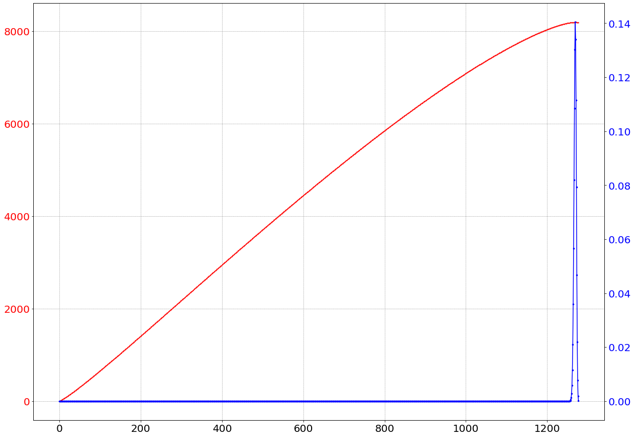
Figure 1: The robdd size distribution of Boolean functions in $13$ variables. The exact distribution is depicted in two ways of presentation: the red curve is the logarithmic scale of the distribution; the blue curve is the probability distribution.

Organization of the paper.

In Section 2 we present the formal notions and objects necessary for the description of our counting approach. Section 3 presents the iterative process for computing the number of robdds having a given profile (the profile describes the number of decision nodes labelled with each variable). Section 3 also states the main result of this paper which is a formula for computing the number of robdds involving linear maps over a polynomial ring. Finally, Section 4 presents the algorithmic context for computing the complete distribution (under the form of the enumerative generating function [6] of robdds).

2 Preliminaries

A Boolean function in $k$ variables is a function from the set $\{{\texttt{0}},{\texttt{1}}\}^{k}$ into the set $\{{\texttt{0}},{\texttt{1}}\}$. The set of functions is denoted by $\mathcal{B}_{k}$ and its cardinality is $2^{2^{k}}$. Furthermore, for the rest of this paper, we choose an ordering of the sequence of variables that corresponds to $x_{1},x_{2},\dots,x_{k}$. Any other ordering could be chosen, but one must be fixed.

2.1 Boolean functions representation

Figure 2 shows a decision tree representing a 4-variable Boolean function and its associated robdd. In both structures, traversing a path from the root to a leaf allows to evaluate the function for a given assignment. Being in a node labelled by $x_{i}$ and going to its low child (using the dotted edge) corresponds with evaluating $x_{i}$ to 0; going to its high child (using the solid edge) corresponds with evaluating $x_{i}$ to 1.

Figure 2: (left) A decision tree and (right) its associated robdd.

Definition 2.1 (dag representation).

Let $f\in\mathcal{B}_{k}$ be a Boolean function in variables $x_{1},\dots,x_{k}$. The function $f$ can be represented as a rooted directed acyclic graph (dag for short) composed of internal decision nodes, labelled by variables and two terminal nodes labelled by $\{\bot,\top\}$ representing respectively the constants 0 and 1. Each decision node labelled by $x_{i}$ has two children, the low child (resp. high child) such that traversing the edge to the low child (resp. high child) corresponds to assign $x_{i}$ to 0 (resp. to 1). The size of a dag is its number of decision nodes.

Definition 2.2 (obdd).

Let $f\in\mathcal{B}_{k}$ and pick one of its dag representation. The dag is called an Ordered Binary Decision Diagram for $f$ (obdd for short) when all paths from the root to a terminal node traverse decision nodes with index in increasing order.

By taking an obdd for a function with a pointed decision node $\nu$ labelled by $x_{i}$, and extracting the sub-dag rooted in $\nu$ by taking all its descendants, we obtain an obdd representing a Boolean function in the variables $x_{i},x_{i+1},\dots,x_{k}$.

Definition 2.3 (robdd).

Let $f\in\mathcal{B}_{k}$ and let $B$ be one of its obdd. If all sub-dags of $B$ are representing distinct Boolean functions, then $B$ is called Reduced Ordered Binary Decision Diagram (robdd).

Figure 3 shows the forbidden configurations in robdd and the operations used to compress the structure.

Figure 3: The two forbidden configurations in robdds and the resulting operations when compressing: (left) $\nu$ and $\nu^{\prime}$ are merged; (right) $\nu$ is deleted (from [7]).

Fact.

Let $f\in\mathcal{B}_{k}$, there exists a single robdd representing $f$.

The data structure of robdds is especially famous due to this property of canonicity. The reader may read Knuth [8] for the proof of uniqueness and several other properties satisfied by robdds.

For the rest of the paper we are only dealing with robdds. Furthermore, we take the point of view of layered robdd by studying and representing robdds layer by layer: each layer contains all decision nodes labelled by the same variable. This layer-by-layer decomposition is natural since the variables are ordered. Thus, a robdd for a function in $k$ variables is composed of $k$ layers (plus a layer for the two terminal nodes). Note that a layer could be empty (which means the Boolean function does not depend on the particular variable associated to this layer).

Definition 2.4 (robdd’s profile).

Let $f\in\mathcal{B}_{k}$ and let $B$ be its robdd. Using the layer-by-layer point of view, we define the profile $B$ to be the non-negative integer sequence $[p_{1},p_{2},\dots,p_{k}]$ such that $p_{i}$ is the number of nodes labelled by $x_{i}$ in $B$, i.e. the size of the layer corresponding to $x_{i}$, for all $i\in\{1,\dots,k\}$.

2.2 Combinatorial description

In our previous paper [3] we proposed a kind of recursive decomposition of a robdd based on the low and high children of the root. Here we propose a new and simpler point of view, based on a layer-by-layer description, which is much more efficient for the counting problem (also for the generating problem). We need to introduce a generalization of a robdd, called multientry robdds, which corresponds exactly to the structure obtained by removing some upper layers in a standard robdd (see Figure 4 for an example).

Informally a multientry robdd is a structure obtained by cutting off a certain number of the top layers of a robdd. The resulting structure is still a dag, but with several sources. We also keep track of where the half-edges from the top layers were pointing. In Figure 4 a robdd and multientry robdd obtained by removing the $3$ top layers are depicted.

Definition 2.5 (Multientry robdd).

A multientry robdd $M$ with at most $k\geq 0$ variables and size $n\geq 0$ is a couple $(M,\mathfrak{E})$. The structure $M$ is a layered dag structure with $n$ decision nodes $\mathcal{Q}$ distributed on $k$ layers and two constant nodes $\{\top,\bot\}$ such that any two subgraphs are non-identical (as in robdds). The multiset $\mathfrak{E}$ has its elements in $\mathcal{Q}\cup\{\top,\bot\}$ and is such that any source node in $M$ (i.e., having in-degree $0$), must appear at least once. The nodes in $\mathfrak{E}$ are called distinguished (and correspond with destination nodes of red half-edges in Figure 4).

As a special case, a robdd is a multientry robdd having one source (the root) and a multiset $\mathfrak{E}$ reduced to the root (with multiplicity $1$).

Figure 4: A robdd of size $13$ (not counting the constant nodes $\{\bot$ and $\top\}$), with $6$ variables and profile $\boldsymbol{p}=[1,2,3,3,3,1]$. (left) A dag representation of the robdd; (right) Cutting off top three layers, we obtain the multientry robdd keeping track with red half edges of nodes which were disconnected.

In the multientry robdd in Figure 4, by numbering the nodes from top to bottom and from left to right, i.e. the leftmost $x_{4}$ is number 1, the second $x_{4}$ is 2, the rightmost $x_{4}$ is 3, the rightmost $x_{5}$ is 4, …, $x_{6}$ is 7 and $\bot$ and $\top$ are respectively 8 and 9, we obtain the multiset $\mathfrak{E}=\{1,2,2,3,4,4,5\}$. We note that our definition of multientry robdd is similar (but not exactly identical) to the one of shared-BDDs presented by Knuth [8] to represent several Boolean functions in the same decision diagram.

Furthermore, remark that the same multientry robdd can be exhibitted by cutting off top layers (not even the same number) of different robdds.

3 Full iterative counting formula

In the following we describe an approach to counting the number of robdds with a given profile $\boldsymbol{p}$. We use a powerful algebraic representation to encapsulate a kind of inclusion-exclusion principle. This motivates the definition of a linear application on polynomials using substitutions. The linearity property of the applications is crucial for achieving our algorithm polynomial complexity. We consider the polynomial ring $\mathbb{Z}[X]$ and linear endomorphisms over $\mathbb{Z}[X]$ (i.e., linear maps between $\mathbb{Z}[X]$ and $\mathbb{Z}[X]$). Thus, for a linear map $g:\mathbb{Z}[X]\to\mathbb{Z}[X]$ and two polynomials $P$ and $Q$ in $\mathbb{Z}[X]$, $g[P+Q]=g[P]+g[Q]$, and for any scalar $\lambda\in\mathbb{Z}$ and polynomial $P\in\mathbb{Z}[X]$ we have $g[\lambda P]=\lambda g[P]$.

In the following theorem, we state the main result of the paper which gives access to the number of multientry robdds for a given profile.

Theorem 3.1 (Multientry robdds counting formula).

For the family of linear maps $(\phi_{r})_{r\geq 0}$, each mapping $\phi_{r}:\mathbb{Z}[X]\to\mathbb{Z}[X]$ is defined with respect to the canonical basis $(X^{m})_{m\geq 0}$ by

$$\phi_{r}[X^{m}]=\left(\prod_{i=0}^{r-1}\left(X^{2}-X-i\right)\right)\cdot\left(\sum_{j=0}^{m-r}\binom{m}{j}\genfrac{\{}{\}}{0.0pt}{}{m-j}{r}\,X^{j}\right).$$ (1)

Let $M(\boldsymbol{p},m)$ be the number of multientry robdds with profile $\boldsymbol{p}=[p_{1},\dots,p_{k}]$ and $m$ incoming half edges. We have, for $k\geq 0$,

$$M(\boldsymbol{p},m)=\left(\phi_{\boldsymbol{p}}[X^{m}]\right)_{X=2},$$ (2)

where

• $\phi_{\boldsymbol{p}}$ is the composition product $\phi_{p_{k}}\circ\phi_{p_{k-1}}\circ\dots\circ\phi_{p_{1}}$;

• for a polynomial $P\in\mathbb{Z}[X]$, $(P)_{X=2}$ is the evaluation of $P$ at $X=2$.

In the theorem, $\binom{m}{j}$ stands for the binomial coefficient and $\genfrac{\{}{\}}{0.0pt}{}{n}{k}$ is the Stirling number of the second kind counting the number ways to partition a set of $n$ objects into $k$ non-empty subsets.

Remark 3.2.

This is actually a stronger result that what we need for counting robdds, since the number of robdds corresponds to the special case where $\boldsymbol{p}=[p_{1}=1,p_{2},\dots,p_{k}]$ and $m=1$ (meaning there is one source node in the top layer). However, the fact that we are able to compute $\phi_{\boldsymbol{p}}$ on the basis $(X^{m})_{m\geq 0}$ is key to our approach.

The detailed the proof of Theorem 3.1 is deferred to after an example of such a computation.

Example.

Let us consider a profile $\boldsymbol{p}=[1,2,4,2]$ for $4$ variables $x_{1},x_{2},x_{3},x_{4}$ and choosing $m=1$ in (2). Then, for $1\leq i\leq 4$, we compute iteratively $\phi_{p_{i}}\circ\dots\circ\phi_{p_{1}}(X)$:

$$X \xmapsto{\phi_{1}}X^{2}-X$$

$$\quad\xmapsto{\phi_{2}}X^{4}-2X^{3}+X$$

$$\qquad\xmapsto{\phi_{4}}X^{8}-4X^{7}+14X^{5}-6X^{4}-16X^{3}+5X^{2}+6X$$

$$\qquad\quad\xmapsto{\phi_{2}}28X^{10}+28X^{9}-98X^{8}-112X^{7}+76X^{6}+92X^{5}-12X^{4}-8X^{3}+6X^{2}.$$

Evaluating the last polynomial at $X=2$, we get that there are $11\,160$ robdds with profile $[1,2,4,2]$. The power of our approach is that we could have stopped at any iteration, and still get the number of robdds for the considered truncated profile. On the particular example this yields

$\boldsymbol{p}$	$\phi_{\boldsymbol{p}}$	$\left(\phi_{\boldsymbol{p}}\right)_{X=2}$
$[\,]$	$X$	$2$
$[1]$	$X^{2}-X$	$2$
$[1,2]$	$X^{4}-2X^{3}+X$	$2$
$[1,2,4]$	$X^{8}-4X^{7}+14X^{5}-6X^{4}-16X^{3}+5X^{2}+6X$	$0$
$[1,2,4,2]$	$28X^{10}+28X^{9}-98X^{8}-112X^{7}+76X^{6}+92X^{5}-12X^{4}-8X^{3}+6X^{2}$	$11\,160$

The number $0$ when considering $[1,2,4]$ may seem counterintuitive at first, but indeed a robdd can only have up to $2$ nodes on its last layer, otherwise one node has to be a duplicate of another.

Proof 3.3 (Proof of Theorem 3.1).

(Multientry robdds counting formula). The proof is obtained by induction on the number $k\geq 0$ of layers with decision nodes.

Base case. When $k=0$ and $n\geq 0$. The number of multientry robdds is $M([\,],m)=2^{m}$, i.e., $X^{m}$ evaluated at $X=2$, as we must map the $m$ half edges to either one of the two constants. Note that if $m=0$ then $M([\,],m)=1$ corresponding to the void function (which is a special case).

Induction step. Now suppose Theorem 3.1 is true for $k\geq 0$.

Let us consider a profile of length $k+1$ as $[r]\cdot\boldsymbol{p}$ with $r\geq 0$ and $\boldsymbol{p}$ a profile of length $k$.

• If $r=0$, a simple computation shows that $\phi_{0}$ is the identity. Hence, the empty layer can in fact be omitted since

  $$\phi_{\boldsymbol{p}}\circ\phi_{0}\left[X^{m}\right]=\phi_{\boldsymbol{p}}\left[X^{m}\right],\quad\text{so that $M([0]\cdot\boldsymbol{p},m)=M(\boldsymbol{p},m)$}.$$ (3)

• From now on let us suppose $0<r\leq m$. The set of $m$ half edges pointing at the first layer can be decomposed in two subsets for $j\in\{0,\dots,m-r\}$: $j$ entries will go to layers below the first one, and $m-j$ entries will be mapped to the $r$ nodes of the first layer. A Stirling number of the second kind $\genfrac{\{}{\}}{0.0pt}{}{n}{k}$ counts the number of ways to partition a set of $n$ objects into $k$ non-empty subsets. So there are $\binom{m}{j}\cdot\genfrac{\{}{\}}{0.0pt}{}{m-j}{r}$ such partitions. We write

  $$M([r]\cdot\boldsymbol{p},m)=\sum_{j=0}^{m-r}\binom{m}{j}\genfrac{\{}{\}}{0.0pt}{}{m-j}{r}f^{(r)}_{\boldsymbol{p}}(j),$$ (4)

  where $f^{(r)}_{\boldsymbol{p}}(j)$ denotes the number of multientry robdds with $j$ free half edges and $r$ pairs of half edges (the ones resulting from the $r$ nodes of the first layer). These $2r$ half edges must thus obey the following constraints:

  • in each pair, the two half edges must be distinct, i.e., point to different nodes;

  • all $r$ pairs of half edges must be distinct with one another (as pairs).

  Our goal now is to get rid of the constraints coming from these $r$ nodes and express all quantities in terms of free half edges.

  The following equation translates the previous constraints on the pair of adjacent half edges coming from the first of the $r$ nodes

  $$f^{(r)}_{\boldsymbol{p}}(j)=f^{(r-1)}_{\boldsymbol{p}}(j+2)-f^{(r-1)}_{\boldsymbol{p}}(j+1)-(r-1)f^{(r-1)}_{\boldsymbol{p}}(j).$$ (5)

  Indeed, the first term $f^{(r-1)}_{\boldsymbol{p}}(j+2)$ corresponds in adding $2$ free half edges, and results in overcounting. Then following an inclusion-exclusion principle, firstly we subtract $f^{(r-1)}_{\boldsymbol{p}}(j+1)$ which would count the number of configurations if the two half edges in this pair were merged. Finally, we subtract $(r-1)f^{(r-1)}_{\boldsymbol{p}}(j)$ in (5). This last quantity counts the number of configurations if the pair of half edges was merged with one of the $r-1$ remaining ones (hence $r-1$ choices). Note that no additional free half edge is added because of this merge. This yields (5).

  Solving the simple recurrence (5) with respect to $r$ yields

  $$f^{(r)}_{\boldsymbol{p}}(j)=\sum_{i=0}^{2r}a_{i}f^{(0)}_{\boldsymbol{p}}(i+j),$$ (6)

  where coefficients $(a_{i})$ are obtained by identifying $P(X)=\prod_{i=0}^{r-1}(X^{2}-X-i)=\sum_{i=0}^{2r}a_{i}X^{i}$.

  At this point, we remark the equality true for $m\geq 0$

  $$M(\boldsymbol{p},m)=f^{(0)}_{\boldsymbol{p}}(m),$$ (7)

  which reflects the fact that in $M(\boldsymbol{p},m)$, all $m$ half edges are unconstrained. Then (4) rewrites

  $$M([r]\cdot\boldsymbol{p},m)=\sum_{j=0}^{m-r}\binom{m}{j}\genfrac{\{}{\}}{0.0pt}{}{m-j}{r}\sum_{i=0}^{2r}a_{i}M(\boldsymbol{p},i+j)=\sum_{i=0}^{m+r}c_{i}M(\boldsymbol{p},i),$$

  with coefficients $c_{i}$ obtained by identifying $\sum_{i=0}^{m+r}c_{i}X^{i}=\phi_{r}(X^{m})$ from (1).

  By induction hypothesis on the length $k$ of $\boldsymbol{p}$ we have for $0\leq i\leq m+r$

  $$M(\boldsymbol{p},i)=\left(\phi_{\boldsymbol{p}}\left[X^{i}\right]\right)_{X=2}.$$ (8)

  By linearity

  $$\sum_{i=0}^{m+r}c_{i}\phi_{\boldsymbol{p}}\left[X^{i}\right]=\phi_{\boldsymbol{p}}\left[\sum_{i=0}^{m+r}c_{i}X^{i}\right]=\phi_{\boldsymbol{p}}\left[\phi_{r}[X^{m}]\right]=\phi_{\boldsymbol{p}}\circ\phi_{r}[X^{m}],$$

  and finally

  $$M([r]\cdot\boldsymbol{p},m)=\sum_{i=0}^{m+r}c_{i}M(\boldsymbol{p},i)=\sum_{i=0}^{m+r}c_{i}\left(\phi_{\boldsymbol{p}}\left[X^{i}\right]\right)_{X=2}=\left(\phi_{\boldsymbol{p}}\circ\phi_{r}[X^{m}]\right)_{X=2}$$

  This ends the proof.

4 Counting algorithms

In this section, we present an algorithm for counting robdds of size $n$.

The time and space complexities are measured respectively in terms of arithmetical operations on $\mathbb{Z}$ and memory space used to store integers in $\mathbb{Z}$. When considering robdds of size upper bounded by $n$, all integers in $\mathbb{Z}$ involved can be checked to be of bit length $O(n\log n)=O(\log n!)$.

The reader can find an implementation of the following algorithms at https://github.com/agenitrini/BDDgen.

4.1 Linear maps: precomputation step

A first step is to pre-compute a representation of linear maps $(\phi_{r})_{r\geq 0}$. For a robdd of size $n$ we know that the maximal number of half edges is $n+1$, and the maximal number of nodes on a layer is also loosely upper bound by $n$. Hence, it is sufficient to compute $\phi_{r}[X^{m}]$ in $\mathbb{Z}[X]$ for $0\leq r\leq n$ and $0\leq m\leq n+1$. In the form of (1), $\phi_{r}[X^{m}]$ is equal to $P_{r}(X)Q_{r,m}(X)$ with

$$P_{r}(X)=\prod_{i=0}^{r-1}(X^{2}-X-i),\quad\text{ and }\quad Q_{r,m}(X)=\sum_{j=0}^{m-r}\binom{m}{j}\genfrac{\{}{\}}{0.0pt}{}{m-j}{r}X^{j}.$$

So the first step is to compute coefficients of $P_{r}(X)$ and $Q_{r,m}(X)$. Concerning binomial coefficient and Stirling numbers of the second kind, both tables can be computed by a naive algorithm (for binomials, it is the famous Pascal’s triangle) in space $O(n^{2})$ with $O(n^{2})$ arithmetic operations on integers.

Once these coefficients are available, we compute the products $\phi_{r}[X^{m}]=P_{r}(X)Q_{r,m}(X)$. Computing $P_{r}$ from $P_{r-1}$ necessitates $O(n)$ arithmetical operations on integers, yielding a total $O(n^{2})$ number of arithmetical operations for the whole family $(P_{r})_{r\leq n}$. Each polynomial $(Q_{r,m})$ necessitates $O(n)$ arithmetical operations per polynomial (supposing binomial coefficients and Stirling number of the second kind are precomputed). Finally, $\phi_{r}[X^{m}]$ is computed with $O(n^{2})$ arithmetical operations (by a naive product of two polynomials). There are $O(n^{2})$ such polynomials to compute. Hence, we get a total $O(n^{4})$ of arithmetic operations using $O(n^{3})$ storage memory space for coefficients. We thus get the next lemma.

Lemma 4.1 (Precomputing step: linear maps).

The precomputation step for the representation of linear maps by computing $\phi_{r}[X^{m}]$ for $0\leq r\leq n$ and $0\leq m\leq n+1$ necessitates $O(n^{4})$ arithmetical operations on integers and uses memory space for $O(n^{3})$ coefficients in $\mathbb{Z}$.

4.2 Basic counting

The basic block in our approach is to be able to compute $\phi_{r}[P]$ for $r\geq 0$. This is done by Algorithm 1 which is a direct translation of Theorem 3.1 using the linearity of the linear maps $(\phi_{r})_{r}$.

Input: an integer $r\geq 0$, a polynomial $P(X)=\sum_{m=0}^{d}p_{m}X^{m}\in\mathbb{Z}[X]$

Output: $\phi_{r}[P]\in\mathbb{Z}[X]$

$Q\leftarrow 0$

for $m$ from $r$ to $d$ do

       $Q\leftarrow Q+p_{m}\phi_{r}[X^{m}]$

      

return $Q$

Algorithm 1 Computing $\phi_{r}[P]$

Input: a profile $\boldsymbol{p}=[p_{1},\dots,p_{k}]$

Output: the number of robdds with profile $\boldsymbol{p}$

$P\leftarrow X$

for $i$ from $1$ to $k$ do

       $P\leftarrow\phi_{p_{i}}[P]$

return $P(2)$

Algorithm 2 Computing $(\phi_{\boldsymbol{p}}[X])_{X=2}$

Proposition 4.2 (Complexity of basic step).

Let $P$ be a polynomial of degree $d$. Algorithm 1 computes $\phi_{r}[P]$ and performs $O(rd+d^{2})$ arithmetical operations over $\mathbb{Z}$ to compute $\phi_{r}[P]$, using $O(d^{2})$ memory space.

Proof 4.3.

Each polynomial $\phi_{r}[X^{m}]$ is of degree $r+m=O(r+d)$. Thus, the number of operations needed on coefficients is $O(rd+d^{2})$ if $r>0$ (or $O(1)$ if $r=0$ since $\phi_{0}$ is the identity).

By Remark 3.2 and applying Theorem 3.1, it is straightforward to compute the number of robdds with profile $\boldsymbol{p}=[p_{1},\dots,p_{k}]$ (using $m=1$). The pseudocode is given in Algorithm 2. We have the following proposition.

Proposition 4.4.

Algorithm 2 computes the number of robdds of size $n$ with $k$ variables and given profile $\boldsymbol{p}$. It performs $O(k\;n^{2})$ arithmetical operations over $\mathbb{Z}$ and uses $O(n)$ extra memory space to store integers.

Proof 4.5.

The number of robdds is $(\phi_{\boldsymbol{p}}[X])_{X=2}$. The polynomial $\phi_{\boldsymbol{p}}[X]$ is computed by iterating $k$ times a linear map of type $\phi_{r}$ starting from an initial polynomial $X$. By Proposition 4.2, the algorithm performs $O(n^{2})$ operations for each iteration since polynomials have $O(n)$ coefficients. The total computation thus performs $O(k\;n^{2})$ arithmetical operations over $\mathbb{Z}$ and use $O(n)$ memory space to store coefficients. Evaluating $(\phi_{\boldsymbol{p}}[X^{m}])_{X=2}$ at $X=2$ can be done in time complexity $O(n)$ (by Horner’s method for instance).

4.3 Generating function for ROBDD size

The main goal of this section is compute the distribution of Boolean functions in $k$ variables according to the robdd size. For $f\in\mathcal{B}_{k}$ a Boolean function, we let $\lambda(f)$ be the size of its robdd, i.e., its number of decision nodes. A convenient way to represent the distribution of the size $\lambda$ on $\mathcal{B}_{k}$ consists in computing the generating function [6]

$$F_{k}(u)=\sum_{f\in\mathcal{B}_{k}}u^{\lambda(f)}=\sum_{i\geq 0}f_{i}u^{i},$$

where $u$ is a formal variable marking the size. Then for $i\geq 0$, the coefficient $f_{i}=[u^{i}]F_{k}(u)$ is the number of robdds of size $i$ with $k$ variables, i.e. the notation $[u^{i}]F_{k}(u)$ corresponds to the coefficient-extraction of the monomial $u^{i}$. We also introduce the truncation $F_{k}^{\leq n}(u)=\sum_{0\leq i\leq n}f_{i}u^{i}$ as the generating functions of robdds of size less than or equal to $n$.

We first extend the formalism introduced in Section 3 and define a linear map $\varphi:\mathbb{Z}[u,X]\to\mathbb{Z}[u,X]$.

Definition 4.6.

The linear map $\varphi:\mathbb{Z}[u,X]\to\mathbb{Z}[u,X]$ is defined via its action on the basis $(u^{r}X^{m})_{r,m\geq 0}$ as

$$\varphi:u^{r}X^{m}\mapsto\varphi[u^{r}X^{m}]=\sum_{i=0}^{m+1}u^{r+i}\phi_{i}[X^{m}].$$ (9)

With this notation we have the following proposition.

Proposition 4.7 (Generating function for robdd size).

The generating function enumerating Boolean functions by considering the robdd size is given by

$$F_{k}(u)=\left(\varphi^{k}[X]\right)_{X=2},\quad\text{where\leavevmode\nobreak\ $\varphi^{k}$ denotes the composition product\leavevmode\nobreak\ $\underbrace{\varphi\circ\dots\circ\varphi}_{\text{$k$ times}}$}.$$

Proof 4.8.

Each application of $\varphi$ corresponds with adding a layer. The formal variable $u$ marks the number of decision nodes added on the current layer.

We remark that in practice we can truncate polynomials, keeping only the terms useful along the computation. The key point here is that if we consider robdds with size bounded by $n$, we should make all computation modulo $u^{n+1}$. Indeed, the formal variable $u$ marks the number of nodes (which is bounded by $n$). Sections A.1 and A.2 int the appendix illustrate this point.

Algorithm 3 computes the bivariate polynomial $\varphi[X^{m}]$ for $m\geq 0$. Algorithm 4, computes recursively the iterated (univariate) version $\left(\varphi^{\ell}[X^{m}]\right)_{X=2}$ (that is the evaluation at $X=2$).

Input: An integer $m\geq 0$

Output: Returns $\varphi[X^{m}]\in\mathbb{Z}[u,X]$

$Q\leftarrow 0$

  $\triangleright$ $Q\in\mathbb{Z}[u]$

for $r$ from $0$ to $m$ do

       $Q\leftarrow Q+u^{r}\phi_{r}[X^{m}]$

return $Q$

Algorithm 3 Computing $\varphi[X^{m}]$

Input: Two integers $\ell,m$

Output: Returns $\left(\varphi^{\ell}[X^{m}]\right)_{X=2}\in\mathbb{Z}[u]$

$\triangleright$ N.B.: Computations done modulo $u^{n+1}$ where $n$ is the maximal size for robdds

if $\ell=0$ then return $2^{m}$

  $\triangleright$ base case

$Q\leftarrow 0$

  $\triangleright$ $Q\in\mathbb{Z}[u]$

$R\leftarrow\varphi(X^{m})$

  $\triangleright$ Call Alg. 3

for $j$ from $0$ to $\operatorname*{deg}_{X}(R)$ do

       $M\leftarrow\left(\varphi^{\ell-1}[X^{j}]\right)_{X=2}$

        $\triangleright$ Call Alg. 4

      $N\leftarrow[X^{j}]\ R(u,X)$

        $\triangleright$ $N\in\mathbb{Z}[u]$

       $Q\leftarrow Q+M\cdot N$

return $Q$

Algorithm 4 Computing $\left(\varphi^{\ell}[X^{m}]\right)_{X=2}$

Lemma 4.9.

Algorithm 3 computes $\varphi[X^{m}]\in\mathbb{Z}[X,u]$, which has $O(n^{2})$ integer coefficients. It performs $O(n^{2})$ arithmetical operations over $\mathbb{Z}$.

Algorithm 4 computes $\left(\varphi^{\ell}[X^{m}]\right)_{X=2}\in\mathbb{Z}[u]$, which has $O(n)$ coefficients. If we omit recursive calls, it performs $O(n^{3})$ arithmetical operations over $\mathbb{Z}$, using memoization techniques with $O((n+k)n^{2})$ extra memory storage.

Proof 4.10.

For Algorithm 3, we perform $m=O(n)$ additions of polynomials in $\mathbb{Z}[X,u]$ with $O(n)$ terms, yielding $O(n^{2})$ arithmetical operations over $\mathbb{Z}$. The result is a bivariate polynomial of bounded degree ($n$ for the variable $u$, $2n$ for the variable $X$) yielding $O(n^{2})$ coefficients. We suppose Algorithm 3 has access to polynomials $\phi_{r}[X^{m}]\in\mathbb{Z}[X]$ from a precomputation step.

For Algorithm 4, two ingredients are essential. Firstly we have to truncate polynomials modulo $u^{n+1}$ so that operations on univariate polynomials have complexity $O(n)$ for addition and $O(n^{2})$ for multiplication (using the naive multiplication on polynomials). Secondly we also use memoization techniques (meaning we compute in lazy manner intermediate results only once and keep it for further reference, at the expense of memory storage). That means that we consider that at the time we compute $\left(\varphi^{\ell}[X^{m}]\right)_{X=2}$, the polynomials $\left(\varphi^{\ell-1}[X^{j}]\right)_{X=2}$ are available (i.e., their complexity is taken into account independently). By an amortizing argument, the complexity of computing the complete family of polynomials $\left(\varphi^{\ell}[X^{m}]\right)_{X=2}$ ($0\leq\ell\leq k$ and $0\leq m\leq n+1$) is still $O(n^{3})$ arithmetical coefficients per polynomial. We need to store $O(kn^{2})$ integer coefficients for memoization of all intermediate polynomials. We also suppose Algorithm 4 has access to bivariate polynomials $(\varphi[X^{m}]\in\mathbb{Z}[u,X])_{0\leq m\leq n+1}$ from a precomputation step which requires $O(n^{3})$ memory space for integer coefficients. A subtle point is to understand that we can truncate polynomials at each step in Algorithm 4 and still get the correct result: this can be proved by recurrence on $\ell$ (see also Section A.2 of the appendix for an example).

Algorithm 4 also computes the generating function of robdds for size up to $n$ since posing $\ell=k$ and $m=1$ we have

$$F_{k}^{\leq n}(u)=\left(\varphi^{\ell}[X]\right)_{X=2}\mod u^{n+1}.$$

Theorem 4.11 (Algorithm for computing the exact distribution).

We compute the generating function $F^{\leq n}_{k}(u)$ of Boolean functions in $\mathcal{B}_{k}$ for robdds of size less than or equal to $n$ using $O(k\;n^{4})$ arithmetical operations in $\mathbb{Z}$ and $O((k+n)\;n^{2})$ for memory space storing integers.

Proof 4.12.

From Lemmas 4.9 and 4.1, the overall complexity is dominated by the computation of the family $(\phi_{r}[X^{m}])_{r,m}$ and the calls to Algorithm 4. By Lemma 4.9, each polynomial $\left(\varphi^{\ell}[X^{j}]\right)_{X=2}$ is computed with $O(n^{3})$ arithmetic operations on integer coefficients and there are $O(k\;n)$ such polynomials. Hence, the total number operations over $\mathbb{Z}$ is $O(k\;n^{4})$. Furthermore, we store $O(k\;n^{2})$ coefficients in $\mathbb{Z}$ for memoization. We also store $O(n^{3})$ coefficients for the family $(\phi_{r}[X^{m}])_{m,r}\in\mathbb{Z}[X]$. This yields the claimed complexity.

To evaluate the complete size distribution we need to consider the size of largest robdds with $k$ variables.

Theorem 4.13 (Maximal size of robdds).

Let $k\geq 1$ be an integer, the maximal number of nodes in a robdd with at most $k$ variables is

$$M_{k}=2^{k-\theta}-3+2^{2^{\theta}},\quad\text{ with\leavevmode\nobreak\ $\theta=\left\lfloor\log_{2}\left(k-\left\lfloor\log_{2}\left(k\right)\right\rfloor\right)\right\rfloor$}.$$

The generating function $F_{k}(u)$ of Boolean functions in $\mathcal{B}_{k}$ according to the robdd size can be computed with $O(2^{4k}/k^{3})$ arithmetical operations in $\mathbb{Z}$ and uses $O(2^{2k}/k)$ space.

Proof 4.14.

Note that this formula is equivalent to the one given without proof by Pontus von Brömssen [13]. The existence of $\theta$ is proved in [12] and from there we can derive the explicit expression of $\theta$. Then substituting $n=M_{k}\approx 2^{k}/k$ in Theorem 4.11 yields the complexity result.

Note this is the polynomial with respect to the maximal size of a robdd for $k$ variables, hence a huge improvement compared to exponential brute force algorithms enumerating all $2^{2^{k}}$ Boolean functions and computing their robdd size obtained after a compaction process. With a careful implementation, we can achieve the computation of $F_{k}(u)$ for $k$ up to $11$ variables on a personal computer, and, on a high-performance computer with $512$ GB RAM memory, for $k=12$ in less than 1 hour 30 minutes, and even for $k=13$ in less than 30 hours using the PyPy implementation of Python.

5 Conclusion

As an application of the counting approach of this paper we are able sample at random robdds. More precisely, we can efficiently and uniformly pick robdds either according to a given size, or even a given profile or a given spine. This is a great improvement when comparing to the classical uniform random generation over the set of Boolean functions, like in [12], that is drastically biased to the largest robdds due to the Shannon effect. For instance with $12$ variables, the probability of drawing uniformly a Boolean function giving a robdd of (quadratic in $k$) size $144=12^{2}$ is approximately $1.212\cdot 10^{-957}$.

In practice, several classical functions have robdds of small size. For example the symmetrical functions in $k$ variables are associated with robdds of quadratic size in $k$ (see [8]). Hence, the approach described in this paper leads the way to provide (polynomial) uniform random generator for robdds of small size (i.e., of size less than exponential).

An interesting future work consists in enumerating the bdd structures where our counting and sampling methods can be applied such as (non-reduced) obdd, or zdd which generally used to represent sets.

Finally, another research direction consists in noting that the generating function of robdds with both size and number of variables can be specified thanks to an iterative process as in Theorem 4.7. It would be interesting to see if the machinery of analytic combinatorics [6] is amenable to this kind of specification.

Appendix A Appendix

A.1 Iterating $\varphi$ (an example)

In this section, we illustrate how $\varphi$ can be iterated to count the distribution of robdds up to $4$ variables. Let us consider the set of Boolean function $\mathcal{B}_{k}$ for $k\in\{1,2,3\}$ and pose $H_{k}(u,X)=\varphi^{k}[X]$.

• $H_{1}(u,X)=\varphi[X]=(\phi_{0}(X)+u\phi_{1}(X))={\left(X^{2}-X\right)}u+X^{2}$. We can verify that substituting $X=2$ we get $F_{1}(u)=H_{1}(u,2)=2\,u+2$. Indeed, $\mathcal{B}_{1}=\{\bot,x_{1},\overline{x_{1}},\top\}$, with respective truth tables $\{\texttt{00},\texttt{01},\texttt{10},\texttt{11}\}$ leading to $2$ robdds of size $1$ and $2$ robdds of size $0$, i.e., with no decision node.

• Adding a second layer, we get $H_{2}(u,X)=\varphi(H_{1}(u,X))=\varphi^{2}[X]$, yielding

  $$H_{2}(u,X)={\left(X^{4}-2\,X^{3}+X\right)}u^{3}+2\,{\left(X^{3}-X^{2}\right)}u^{2}+2\,{\left(X^{2}-X\right)}u+X.$$

  We get $F_{2}(u)=2\,u^{3}+8\,u^{2}+4\,u+2$, hence there are $2,8,4,2$ robdds of respective sizes $3,2,1$ and $0$ for $16$ Boolean functions on $2$ variables.

• Iterating with a third layer, we get $H_{3}(u,X)=\varphi(H_{1}(u,X))=\varphi^{3}[X]$ which has $34$ terms and gives

  $$F_{3}(u)=74\,u^{5}+88\,u^{4}+62\,u^{3}+24\,u^{2}+6\,u+2.$$

  Hence, there are respectively $74,88,62,24,6$ and $2$ robdds of size $5,4,3,2,1$ and $0$.

• Adding a fourth layer yields for $H_{4}(u,X)=\varphi^{k}[X]$ a polynomial with $134$ terms and

  $$F_{4}(u)=11160\,u^{9}+23280\,u^{8}+17666\,u^{7}+8928\,u^{6}+3248\,u^{5}+960\,u^{4}+236\,u^{3}+48\,u^{2}+8\,u+2.$$

  There are $11160$ robdds with $4$ variables of size $9$, $23280$ robdds of size $8$, etc.

Of course, we can check that $F_{k}(1)=2^{2^{k}}$, which is the number of Boolean functions on $k$ variables.

A.2 Truncating polynomials (an example)

In this subsection, we illustrate on an example the computational effect of truncating polynomials.

Let us consider that the generating function $F_{3}^{\leq 3}(u)\leavevmode\nobreak\$ of robdd with $k=3$ variables and with less or equal to $n=3$ decision nodes. The maximal size of a robdd for $k=3$ variables is $M_{3}=7$ ($7$ decision nodes). Then $\varphi^{3}[X]$ is a polynomial with $34$ terms. We can write (terms who would disappear modulo $u^{n+1}=u^{4}$ are grayed)

$$\varphi^{3}[X] ={\color[rgb]{.5,.5,.5}\left(X^{8}-4\,X^{7}+14\,X^{5}-6\,X^{4}-16\,X^{3}+5\,X^{2}+6\,X\right)u^{7}}$$

$${\color[rgb]{.5,.5,.5}+4\,{\left(X^{7}-2\,X^{6}-3\,X^{5}+5\,X^{4}+4\,X^{3}-3\,X^{2}-2\,X\right)}u^{6}}$$

$${\color[rgb]{.5,.5,.5}+{\left(8\,X^{6}-12\,X^{5}-11\,X^{4}+14\,X^{3}+4\,X^{2}-3\,X\right)}u^{5}}$$

$${\color[rgb]{.5,.5,.5}+2\,{\left(5\,X^{5}-6\,X^{4}-5\,X^{3}+4\,X^{2}+2\,X\right)}u^{4}}$$

$$+{\left(9\,X^{4}-10\,X^{3}-2\,X^{2}+3\,X\right)}u^{3}$$

$$+6\,{\left(X^{3}-X^{2}\right)}u^{2}$$

$$+3\,{\left(X^{2}-X\right)}u$$

$$+X$$

Truncating modulo $u^{4}$ and substituting $X=2$ yields the polynomial

$$F_{3}^{\leq 4}(u)=62\,u^{3}+24\,u^{2}+6\,u+2.$$

The problem of computing all the terms before truncating the result is that there are $O(\frac{2^{2k}}{k^{2}})$ terms (since $M_{k}\approx 2^{k}/k$), hence a combinatorial explosion.

In contrast, Algorithm 4 works in a recursive manner and truncate polynomials along the way so that we have a polynomial number of terms. In the following, we describe with some details how to compute $(\varphi^{3}(X))_{X=2}$.

First, Algorithm 4 decomposes $(\varphi^{3}(X))_{X=2}$ as $(\varphi^{2}\circ\varphi[X]))_{X=2}$. In general, $\varphi[X^{m}]$ is a polynomial of respective degree $m$ and $2m$ in variables $u$ and $X$ and has $O(m^{2})$ integer coefficients. We compute (collecting terms with respect to variable $X$)

$$\varphi[X]=(X^{2}-X)u+X=X^{2}u+X(1-u).$$ (10)

Denoting $B^{(2)}_{m}(u)=(\varphi^{2}[X^{m}])_{X=2}$, our algorithm computes recursively for the basis $(1,X,X^{2})$ (removed monomials modulo $u^{4}$ ar grayed)

$$B^{(2)}_{0}(u) =1$$

$$B^{(2)}_{1}(u) =2\,u^{3}+8\,u^{2}+4\,u+2$$

$$B^{(2)}_{2}(u) ={\color[rgb]{.5,.5,.5}74\,u^{4}}+90\,u^{3}+68\,u^{2}+20\,u+4$$

Then since $\varphi$ is linear, we compute (still modulo $u^{4}$) using Equation (10)

$$(\varphi^{3}(X))_{X=2} =B_{2}(u)u+B_{1}(u)(1-u)$$

$$=u(90\,u^{3}+68\,u^{2}+20\,u+4)+(1-u)(2\,u^{3}+8\,u^{2}+4\,u+2)$$

$$={\color[rgb]{.5,.5,.5}88\,u^{4}}+62\,u^{3}+24\,u^{2}+6\,u+2.$$

In summary, computing modulo $u^{n+1}$ along the process allows us to control the degree $O(n)$ of polynomials involved, which in turn ensures that the computation stays of polynomial complexity (with respect ti arithmetical operations on integers).

Observing such curves for $k$ from $1$ to $13$, we notice the exponential growth of the largest robdds when the number $k$ of variables increases. Indeed, in Theorem 4.13 we define $M_{k}$ to be the size of the largest robdds with $k$ variables. The sequence starts as $(M_{k})_{k=1,\dots,13}=(1,3,5,9,17,29,45,77,141,269,509,765,1277).$

References

- [1] R. E. Bryant. Graph-Based Algorithms for Boolean Function Manipulation. IEEE Trans. Computers, 35(8):677–691, 1986.
- [2] R. E. Bryant. Symbolic Boolean Manipulation with Ordered Binary-Decision Diagrams. ACM Comput. Surv., 24(3):293–318, 1992.
- [3] J. Clément and A. Genitrini. Binary decision diagrams: From tree compaction to sampling. In LATIN: Theoretical Informatics - 14th Latin American Symposium, Proceedings, volume 12118 of LNCS, pages 571–583. Springer, 2020.
- [4] A. Darwiche and P. Marquis. A knowledge compilation map. J. Artif. Int. Res., 17(1):229–264, sep 2002.
- [5] R. Drechsler, A. Sarabi, M. Theobald, B. Becker, and M. A. Perkowski. Efficient Representation and Manipulation of Switching Functions Based on Ordered Kronecker Functional Decision Diagrams. In DAC’94, pages 415–419, 1994.
- [6] P. Flajolet and R. Sedgewick. Analytic Combinatorics. Cambridge University Press, New York, NY, USA, 1 edition, 2009.
- [7] C. Gröpl, H. J. Prömel, and A. Srivastav. Ordered binary decision diagrams and the shannon effect. Discret. Appl. Math., 142(1-3):67–85, 2004. doi:10.1016/j.dam.2003.02.003.
- [8] D. E. Knuth. The Art of Computer Programming, Volume 4A, Combinatorial Algorithms. Addison-Wesley Professional, 2011.
- [9] L. Kruger, S. Jha, E.-J. Goh, and D. Boneh. Secure Function Evaluation with Ordered Binary Decision Diagrams. In CCS’06, pages 410–420. ACM, 2006.
- [10] S.-I. Minato. Zero-Suppressed BDDs for Set Manipulation in Combinatorial Problems. 30th ACM/IEEE Design Automation Conference, pages 272–277, 1993.
- [11] C. Mues, B. Baesens, C. M. Files, and J. Vanthienen. Decision diagrams in machine learning: an empirical study on real-life credit-risk data. Expert Systems with Applications, 27(2):257–264, 2004.
- [12] J. Newton and D. Verna. A theoretical and numerical analysis of the worst-case size of reduced ordered binary decision diagrams. ACM TCL, 20(1):6:1–6:36, 2019.
- [13] N. J. A. Sloane. The On-Line Encyclopedia of Integer Sequences, Sep 2019. Sequence A327461.
- [14] J. Vuillemin and F. Béal. On the BDD of a Random Boolean Function. In ASIAN’04, pages 483–493, 2004.
- [15] I. Wegener. The size of reduced OBDDs and optimal read-once branching programs for almost all Boolean functions. In GTCCS’94, pages 252–263, 1994.
- [16] I. Wegener. Branching Programs and Binary Decision Diagrams. SIAM, 2000.