Detection of Sparse Anomalies in
High-Dimensional Network Telescope Signals

Abstract

Network operators are increasingly overwhelmed with incessant cyber-security threats, ranging from malicious network reconnaissance to attacks such as distributed denial of service and data breaches. A large number of these attacks could be prevented if the network operators were better equipped with threat intelligence information that would allow them to block nefarious scanning activities. Network telescopes or “darknets” offer a unique window into observing Internet-wide scanners and other malicious entities, and they could offer early warning signals to operators that would be critical for infrastructure protection. Hence, monitoring network telescopes for timely detection of coordinated and heavy scanning activities is an important, albeit challenging, task. The challenges mainly arise due to the non-stationarity and the dynamic nature of Internet traffic and, more importantly, the fact that one needs to monitor high-dimensional signals (e.g., all TCP/UDP ports) to search for “sparse” anomalies. We propose statistical methods to address both challenges in an efficient and “online” manner; our work is validated both with synthetic data and with real-world data from a large network telescope.

I Introduction

The Internet has evolved into a complex ecosystem, comprised of a plethora of network-accessible services and end-user devices that are frequently mismanaged, not properly maintained and secured, and outdated with untreated software vulnerabilities. Adversaries are increasingly becoming aware of this ill-secure Internet landscape and leverage it to their advantage for launching attacks against critical infrastructure. Examples abound: foraging for mismanaged NTP and DNS open resolvers (or other UDP-based services) is a well-known attack vector that can be exploited to incur volumetric reflection-and-amplification distributed denial of service (DDoS) attacks [1, 2, 3]; searching for and compromising insecure Internet-of-Things (IoT) devices (such as home routers, Web cameras, etc.) has led to the outset of the Mirai botnet back in 2016 that was responsible for some of the largest DDoS ever recorded [4, 5, 6, 7]; variants of the Mirai epidemic still widely circulate (e.g., the Mozi [8] and Meri [9] botnets) and assault services at a global scale; cybercriminals have been exploiting the COVID-19 pandemic to infiltrate networks via insecure VPN teleworking technologies that have been deployed to facilitate work-from-home opportunities [10].

Notably, the initial phase of the aforementioned attacks is network scanning, a step that is necessary to detect and afterwards exploit vulnerable services/hosts. Against this background, network operators are tasked with monitoring and protecting their networks and germane services utilized by their users. While many enterprises and large-scale networks operate sophisticated firewalls and intrusion detection systems (e.g., Zeek, Suricata or other non-open-source solutions), early signs of malicious network scanning activities may not be easily noticed from their vantage points. Large Network Telescopes or Darknets [11, 12], however, can fill this gap and can provide early warning notifications and insights for emergent network threats to security analysts. Network telescopes consist of monitoring infrastructure that receives and records unsolicited traffic destined to vast swaths of unused but routed Internet address spaces (i.e., millions of IPs). This traffic, coined as “Internet Background Radiation” [13, 14], captures traffic from nefarious actors that perform Internet-wide scanning activities, malware and botnets that aim to infect other victims, “backscatter” activities that denote DoS attacks [14], etc. Thus, Darknets offer a unique lens into macroscopic Internet activities and timely detection of new abnormal Darknet behaviors is extremely important.

In this paper, we consider Darknet data from the ORION Network Telescope operated by Merit Network, Inc. [12], and construct multivariate signals for various TCP/UDP ports (as well as other types of traffic) that denote the amount of packets sent to the Darknet towards a particular port per monitoring interval (e.g., minutes). (See Figure 1.) Our goals are to detect when an “anomaly” occurs in the Darknet and to also accurately identify the culprit port(s); such threat intelligence would be invaluable in diagnosing emerging new vulnerabilities (e.g., “zero-day” attacks). Our algorithms are based on the state-of-the-art theoretical results on the sparse signal support recovery problem in a high-dimensional setting (see, e.g., [15] and the recent monograph [16]). Our main contributions are: 1) we showcase, using simulated as well as real-world Darknet data, that signal trends (e.g., diurnal or weekly scanning patterns) can be filtered out from the multi-variate scanning signals using efficient sequential PCA (Principal Component Analysis) techniques [17]; 2) using recent theory [15], we demonstrate that simple thresholding techniques applied individually on each univariate time-series exhibit better detection power than competing methods proposed in the literature for diagnosing network anomalies [18]; 3) we propose and apply a non-parametric approach as a thresholding mechanism for the recovery of sparse anomalies; and 4) we illustrate our methods on real-world Darknet data using techniques amenable to online/streaming implementation.

II Related Work

Network telescopes have been widely employed by the networking community to understand various macroscopic Internet events. E.g., Darknet data helped to shed light into botnets [4, 19], to obtain insights about network outages [20, 21], to understand denial of service attacks [22, 23, 1], for examining the behavior of IoT devices [24], for observing Internet misconfigurations [25, 14], etc.

Mining of meaningful patterns in Darknet data is a challenging task due to the dimensionality of the data and the heterogeneity of the “Darknet features” that one could invoke. Several studies have resorted to unsupervised machine learning techniques, such as clustering, for the task at hand. Niranjana et al. [26] propose using Mean Shift clustering algorithms on TCP features to cluster source IP addresses to find attack patterns in Darknet traffic. Ban et al. [27] present a monitoring system that characterizes the behavior of long term cyber-attacks by mining Darknet traffic. In this system, machine learning techniques such as clustering, classification and function regression are applied to the analysis of Darknet traffic. Bou-Harb et al. [28] propose a multidimensional monitoring method for source port 0 probing attacks by analyzing Darknet traffic. By performing unsupervised machine learning techniques on Darknet traffic, the activities by similar types of hosts are grouped by employing a set of statistical-based behavioral analytics. This approach is targeted only for source port 0 probing attacks. Nishikaze et al. [29] present a machine learning approach for large-scale monitoring of malicious activities on Internet using Darknet traffic. In the proposed system, network packets sent from a subnet to a Darknet are collected, and they are transformed into 27-dimensional TAP (Traffic Analysis Profile) feature vectors. Then, a hierarchical clustering is performed to obtain clusters for typical malicious behaviors. In the monitoring phase, the malicious activities in a subnet are estimated from the closest TAP feature cluster. Then, such TAP feature clusters for all subnets are visualized on the proposed monitoring system in real time to identify malicious activities. Ban et al. [30] present a study on early detection of emerging novel attacks. The authors identify attack patterns on Darknet data using a clustering algorithm and perform nonlinear dimension reduction to provide visual hints about the relationship among different attacks.

Another family of methods rely on traffic prediction to detect anomalies. E.g., Zakroum et al. [31] infer anomalies on network telescope traffic by predicting probing rates. They present a framework to monitor probing activities targeting network telescopes using Long Short-Term Memory deep learning networks to infer anomalous probing traffic and to raise early threat warnings.

III Methodology

III-A Problem Formulation

Consider a vector time series ${\bm{x}}_{t}=\{x_{t}(i)\}_{i=1}^{p}$ modelling a collection of $p$ data streams (e.g., scanning activity against $p$ ports). In network traffic monitoring applications, the data streams involve a highly non-stationary “baseline” traffic background signal ${\bm{\theta}}_{t}=\{\theta_{t}(i)\}_{i=1}^{p},$ which could be largely unpredictable and highly variable. Considering Internet traffic specifically, this “baseline” traffic often includes diurnal or weekly periodic trends that can be modeled by a small number of common factors. We encode these periodic phenomena through the classic linear factor model. Namely, we make the assumption that ${\bm{\theta}}_{t}=B{\bm{f}}_{t},$ where $B=({\bm{b}}_{1}\ldots{\bm{b}}_{k})_{p\times k}$ is a matrix of $k(\leq p)$ linearly independent columns that expresses the affected streams. Moreover, ${\bm{f}}_{t}=\{f_{t}(j)\}_{j=1}^{k}$ are the (non-stationary) factors, or periodic trends, that appear in these different streams. That is, the anomaly free regime can be modeled as

$${\bm{x}}_{t}=B{\bm{f}}_{t}+{\bm{\epsilon}}_{t},$$ (1)

where ${\bm{\epsilon}}_{t}=\{\epsilon_{t}(i)\}_{i=1}^{p}$ is a vector time-series modeling the “benign” noise. The time-series $\{{\bm{\epsilon}}_{t}\}$ may and typically does have a non-trivial (long-range) dependence structure [32], but may be assumed to be stationary.

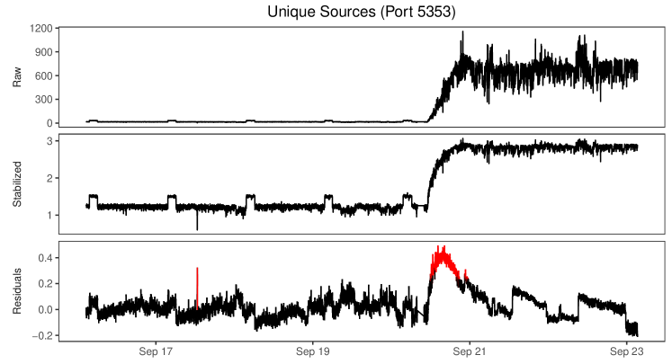
Figure 1: (a) Incoming unique source IP traffic coming to port 5353, from 16 September, 0639 UTC to 23 September, 0719 UTC in 2016. (b) Incoming traffic for the same port after stabilization through log-transform. Another event is now visible despite diurnal trends in traffic denoted by a spike around 17 September 14:00 UTC. (c) Residuals for the same port from the traffic model. The large event is flagged by our algorithm. Our method adapts to the change of regime after the second event and does not flag the whole remaining time series as anomaly. Moreover, the periodic trend until 21 September is clearly filtered out after the application of the algorithm.

Anomalies such as aggressive network scanning may be represented (in a suitable feature space) by a mean-shift vector ${\bm{u}}_{t}=\{u_{t}(i)\}_{i=1}^{p}$, which is sparse, i.e., it affects only a relatively small and unknown subset of streams $S_{t}:=\{i\in[p]:u_{t}(i)\neq 0\}.$ Thus, in the anomalous regime, one observes

$${\bm{x}}_{t}=B{\bm{f}}_{t}+{\bm{u}}_{t}+{\bm{\epsilon}}_{t}.$$ (2)

The general problems of interest are twofold:

• Detection: Timely detection of the presence of the anomalous component ${\bm{u}}_{t}.$

• Identification: The estimation of the sets $S_{t}$ of the streams containing anomalies.

III-B An Algorithm for Joint Detection and Identification

We provide a high level summary of the algorithm we implement in our analysis. We examine high-dimensional data sourced from Darknet traffic observations and our goal is the joint detection and identification of any nefarious activity that might be present in the dataset.

In order to achieve our goals, we utilize sequential PCA techniques (i.e., incremental PCA or iPCA) attempting to estimate the factor subspace spanned by the common periodic trends. Once an estimate of this space is obtained, we project the new vector of data (one observation in each port signal) on this subspace and retain the residuals of the data minus their projections. Using an individual threshold for each stream, pertaining to the stream’s marginal variance and a control limit chosen by the operator (see Section IV-A3 for guidance in system tuning), observations are flagged as anomalies individually.

Algorithm 1 Online identification of sparse anomalies

smoothing parameters $\lambda,\lambda_{\mu},\lambda_{\sigma}$;

control limit $L$; effective subspace dimension $k$;

initial subspace estimates $\widehat{B}$; initial mean estimates $\widehat{{\bm{\nu}}}_{x},\widehat{{\bm{\nu}}}_{r}$

initial residual marginal variance estimates $\widehat{{\bm{\sigma}}}^{2}_{r}$,

iPCA forget factor $\eta$, robust estimation guard $R$.

for new data ${\bm{x}}_{t}=(x_{t}(j))_{j=1}^{p}\in\mathrm{R}^{p}$ do

     for $j\not\in\widehat{S}_{t-1}$ do

         $\widehat{\nu}_{x}(j)\leftarrow(1-\lambda)\widehat{\nu}_{x}(j)+\lambda x_{t}(j)$ $\triangleright$ Update mean estimates

     end for

     ${\bm{r}}_{t}\leftarrow(I-\widehat{B}(\widehat{B}^{\top}\widehat{B})^{-1}\widehat{B}^{\top})({\bm{x}}_{t}-\widehat{{\bm{\nu}}}_{x})$ $\triangleright$ Projection step

     $\widehat{B}\leftarrow\mathrm{iPCA}({\bm{x}}_{t},\widehat{B},\widehat{{\bm{\nu}}}_{x},k)$ $\triangleright$ Update subspace

     for $j$: $|r_{t}(j)|<R\cdot\widehat{\sigma}_{r}(j)$ do

         $\widehat{\nu}_{r}(j)\leftarrow(1-\lambda_{\mu})\widehat{\nu}_{r}(j)+\lambda_{\mu}r_{t}(j)$

     end for

     for $j$: $|r_{t}(j)-\widehat{\nu}_{r}(j)|<R\cdot\widehat{\sigma}_{r}(j)$ do

         $\widehat{\sigma}^{2}_{r}(j)\leftarrow(1-\lambda_{\sigma})\widehat{\sigma}^{2}_{r}(j)+\lambda_{\sigma}(r_{t}(j)-{\widehat{\nu}_{r}(j)})^{2}$

$\triangleright$ Update residual variances

     end for

     $\widehat{S_{t}}\leftarrow\{j\;|\;|r_{t}(j)-\widehat{\nu}_{r}(j)|>L\times\widehat{\sigma}(j)\}$

     if $\widehat{S_{t}}\neq\;$Ø then

         Raise alert on $\widehat{S_{t}}$

     end if

end for

The algorithm can be broken down in five phases.

1. Input. Tuning parameters include the length of the warm-up period ($n_{0}$) and smoothing parameters for some Exponentially Weighted Moving Average (EWMA) steps [33]; $\lambda,\lambda_{\mu},\lambda_{\sigma}$ denote the memory parameters for the EWMA of the mean of the data ${\bm{x}}_{t}$, the mean of the residuals ${\bm{r}}_{t}$ and the marginal variance of the residuals $(\widehat{{\bm{\sigma}}}_{r}^{2})$. Additionally, the memory parameter of the incremental PCA (iPCA) (namely, $\eta$) can be chosen by the user. Moreover, one can choose the control limit $L$, used in the alert phase, the variance cut-off percentage $\pi$ and the robust guard estimation (REG) parameter $R$, controlling the sequential update of the EWMAs.

2. Initialization. The “warm-up” dataset, undergoes a batch PCA. Using the percentage $\pi$ that denotes the fraction of variance “explained”, one can determine the effective dimension $k$ of the factor subspace to be estimated, which dictates the trends that would be filtered out. The mean of the data $(\widehat{{\bm{\nu}}}_{x})$, the mean $(\widehat{{\bm{\nu}}}_{r})$ and the marginal variance $(\widehat{{\bm{\sigma}}}_{r}^{2})$ of the residuals are initialized based on the training data.

3. Sequential Update. A new vector of data $({\bm{x}}_{t})$ is observed and passed through the algorithm. We update the estimated factor subspace $\widehat{B}$ using incremental PCA [17]. The vector $\widehat{{\bm{\nu}}}_{x}$ is updated using EWMA.

4. Residuals. Depending on whether there is an ongoing anomaly, we center ${\bm{x}}_{t}$. We project the centered data onto the orthogonal complement of $\widehat{B}$ and obtain the residual $({\bm{r}}_{t})$. If any coordinate of ${\bm{r}}_{t}$ is smaller in magnitude than $R$ times the marginal variance, then the appropriate elements of both $\widehat{{\bm{\nu}}}_{r}$ and $\widehat{{\bm{\sigma}}}_{r}^{2}$ are updated via EWMA.

5. Alerts. Finally, if any coordinate in the centered residuals exceeds in magnitude the corresponding element in $L\times\widehat{{\bm{\sigma}}}_{r}$, an alert is raised.

There are two important points that we would like to make regarding the effectiveness of the proposed Algorithm.

• First, non-stationarity in the form of e.g. diurnal cycles in the data is absorbed in the projection step, and not with a time-series model.

• The sparse anomalous signals remain largely unaffected by the projection step. This can be quantified with the help of an incoherence condition (see Proposition III.2 and its proof in Section V) that is generally satisfied in network traffic monitoring problems. This then leaves us with the residuals approximating the signals

  $${\bm{r}}_{t}\approx{\bm{u}}_{t}+{\bm{\epsilon}}_{t},$$ (3)

  and enables us to detect and locate sparse anomalies.

Moreover, the sequentially and non-parametrically updated estimate of the variance $\widehat{{\bm{\sigma}}}_{r}^{2}$ on Step (4) of the algorithm can be shown to be a consistent estimator in the special case that our residuals $\{{\bm{r}}_{t}\}_{t=1}^{\infty}$ form a Gaussian time series. (More general cases could be examined as future work.) Indeed, let $\{{r}_{t}(j),\ t\in\mathbb{Z},\ j\in[p]:=\{1,\dots,p\}\}$ be a zero-mean stationary Gaussian time series, with some correlation structure

$$\rho_{t}(j)={\rm Cor}({r}_{t}(j),{r}_{0}(j))={\rm Cor}({r}_{t+h}(j),{r}_{h}(j)),$$ (4)

for $\ t\in\mathbb{Z},\ j\in[p],\ \forall h\in\mathbb{Z}$. We propose the estimator

$$\widehat{{\sigma}}_{t}^{2}(j)=(1-\lambda_{\sigma})\widehat{{\sigma}}_{t-1}^{2}(j)+\lambda_{\sigma}{r}_{t}^{2}(j),$$ (5)

in order to estimate the unknown variance of ${\bm{r}}_{t}$ non-parametrically. Namely for the estimation of this variance, we implement an EWMA on the squares of the zero-mean stationary series $\{{\bm{r}}_{t},\ t\in\mathbb{Z}\}$, which the following Proposition III.1 proves consistent.

Proposition III.1.

Let $\{\widehat{\sigma}_{t}^{2},\ t\in\mathbb{Z}\}$ be defined as in (5) and $\{\rho_{t},t\in\mathbb{Z}\}$ as in (4) (we have dropped the index $j$ to keep the notation uncluttered). If $\sum_{t=-\infty}^{\infty}\rho_{t}^{2}<\infty$, then the estimator $\widehat{\sigma}_{t}^{2}$ is consistent.

Remark 1.

Note that at first glance the EWMA estimator for the variance of the residuals in (5) seems inconsistent with the one in Algorithm 1, due to the lack of the centering term $\widehat{\nu}_{r}(j)$. Recall that our method firstly projects the original data in the orthogonal complement of the estimated subspace $\widehat{B}$, obtaining the residuals $\widehat{{\bm{r}}}_{t}$, which are then centered. The centered residuals correspond to the residuals that we utilize in the proof and setting of Proposition III.1, i.e., we assume they are a zero-mean Gaussian stationary time series with square summable correlation structure. Thus, the update of $\widehat{\sigma}_{r}^{2}(j)$ in (5) does not require the existence of a centering factor.

We now proceed to elaborate on the incoherence condition, which ensures that the sparse anomalies are largely retained by the projection step.

III-C Incoherence conditions

Disentangling sparse errors from low rank matrices has been a topic of extensive research since the last decade. While there are seminal works on recovering sparse contamination from a low-rank matrix exactly, they all resort to solving a convex program or a program with convex regularization terms [34, 35, 36]. The form that most closely resembles the set-up of our problem is Zhou et.al. [37], where the model has both a Gaussian error term and a sparse corruption; see also Xu et.al.[36], Candes et.al. [35] and references therein.

This line of literature often criticizes the classical PCA in the face of outliers and data corruptions. However, to the best of our knowledge, there has been no analysis documenting just how or when the classical PCA becomes brittle in recovering sparse errors when the training period itself is contaminated. Our empirical and theoretical findings point to the contrary.

Secondly, rarely can such convex optimization-based methods be made “online”. Our approach here is to separate sparse errors from streaming data rather than stacked vectors of observations (i.e., measurement matrices) collected over long stretches of time. The low-rank matrix completion line of work faces challenges when data comes in streams rather than in batches, because the matrix nuclear norm often used in such problems closely couples all data points. In a notable effort by Feng, Xu, and Yan [38] an iterative algorithm was proposed to solve the optimization problem with streaming data. However, implementing the algorithm requires extensive calibration and tuning which makes it impractical for non-stationary data streams with ever-shifting structures.

We now make formal the following statement: under the suitable structural assumption on the factor loading matrix $B$ stated below, PCA is still a resilient tool for recovery of the low-rank component and the sparse errors on observations ${\bm{x}}_{t}$. Our results provide theoretical guarantees on the error in recovering the locations and magnitudes of sparse anomalies.

We analyze the faithfulness of residuals in (3) in recovering sparse anomalies under the following assumptions.

$$\lambda_{\mathrm{min}}(B^{\top}B)\geq\phi(p),\text{ for some function }\phi\text{ of }p.$$ (6)

Entries of $B$ are bounded by a constant $C$, uniformly in $p$:

$$|B(i,j)|\leq C,\quad\forall i\in[p]:=\{1,\dots,p\},j\in[k]$$ (7)

Conditions (6) & (7) are closely linked to the so-called incoherence conditions in high-dimensional statistics [34]. Notice that for (6) and (7) to hold simultaneously, we need $\phi(p)\leq Cp$. These conditions are important for the theoretical guarantees in the high-dimensional asymptotics regime where $p\to\infty$ but in practice they are quite mild and natural.

Condition (6) ensures that the background signal in the factor model $B{\bm{f}}_{t}$ has enough energy or a “ground-clearance” relative to the dimension. In the context of Internet traffic monitoring, this is not a restrictive condition since otherwise the background signal can be modeled with a lower-dimensional factor model with smaller value of $k$. The second assumption (7), taken together with (6) ensures that the columns of $B$ are not sparse and consequently the background traffic is not concentrated on one or a few ports. This is also natural. Indeed, if the background was limited to a sparse subset of ports, then they would always behave differently than the majority of the ports and one can simply analyze these ports separately using a lower-dimensional model with smaller value of $p$, where we no longer have sparse background.

Let now $\Sigma=BB^{\top}$ and $\widehat{\Sigma}$ be an estimate of $\Sigma$ obtained for example, by performing iPCA and taking the top-$k$ principal components. (Alternatively, one simply take $\widehat{\Sigma}:=n^{-1}\sum_{t=1}^{n}{\bm{x}}_{t}{\bm{x}}_{t}^{\top}$, for a window of $n$ past observations.)

Proposition III.2 (Resilience of PCA).

Assume (6) and (7) hold. Then, for any $k$ and $p$, and for each coordinate $i\in[p]$,

$${\mathbb{E}}(r_{t}(i)-(\epsilon_{t}(i)+u_{t}(i)))^{2}\leq\\ \Bigg{[}\left({\mathbb{E}}\|\widehat{\Sigma}-\Sigma\|^{2}\right)^{1/2}\frac{2\sqrt{kp}}{\phi(p)}\left(c_{f}Ck+1+\sqrt{\frac{\mbox{tr}(\Sigma_{u})}{p}}\right)\\ +\frac{\sqrt{k}C}{\phi(p)}\left(1+\sqrt{kp}C\|\Sigma_{u}\|^{1/2}\right)\Bigg{]}^{2}$$ (8)

where $\Sigma_{{u}}={\mathbb{E}}[{\bm{u}}_{t}{\bm{u}}_{t}^{\top}]$ and $\|{\bm{f}}_{t}\|\leq c_{f}\sqrt{k}$.

This result, under the conditions of Proposition V.3, shows that if $p^{5/2}=o(\phi(p))$, with $k$ and $\Sigma_{{u}}$ bounded, the upper bound in (8) converges to zero, as the dimension $p$ grows. That is, the anomaly signal ${\bm{u}}_{t}$ “passes through” to the residuals ${\bm{r}}_{t}$ and the approximation in (3) can be quantified. Indeed, assuming $k$ is fixed for a moment, (8) entails that the point-wise bound on mean-squared difference between the unobserved anomaly-plus-noise signal $u_{t}(i)+\epsilon_{t}(i)$ and the residuals $r_{t}(i)$ obtained from our algorithm is ${\cal O}({\mathbb{E}}(\|\widehat{\Sigma}-\Sigma\|^{2})p/\phi^{2}(p))$. This means that in practice, anomalies $u_{t}(i)$ of magnitudes exceeding $p^{5/2}/\phi(p)$ will be present in the residuals $r_{t}(i)$. As seen in the lower bound in (12) this is a rather mild restriction. Thus, in view of Theorem III.3, provided $\phi(p)\gg\sqrt{p/\log(p)}$, the theoretically optimal exact identification of all sparse anomalies is unaffected by the background signal $B{\bm{f}}_{t}$.

In practice, however, the key caveat is the accurate estimation of $\Sigma$, which can be challenging if the noise ${\bm{\epsilon}}_{t}$ and/or the factor signals ${\bm{f}}_{t}$ are long-range dependent. In Proposition V.3 we establish upper bounds on ${\mathbb{E}}[\|\widehat{\Sigma}-\Sigma\|^{2}]$ via the Hurst long-range dependence parameter of the time-series $\{\epsilon_{t}(i)\},$ conditions on $\{f_{t}\}$, and the length of the training window $n$, while the time-series $\{u_{t}(i)\}$ is also assumed long-range dependent. It shows that even in the presence of long-range dependence, provided the training window and the memory of iPCA are sufficiently large, the background signal can be effectively filtered out without affecting the theoretical boundary for exact support recovery discussed in the next section.

III-D Statistical Limits in Sparse Anomaly Identification

As argued in the previous section using for example PCA-based filtering methods, one can remove complex non-sparse spatio-temporal background/trend signal without affecting significant sparse anomalies. Therefore, the sparse anomaly detection and identification problems can be addressed transparently in the context of the signal-plus-noise model. Namely, assume that we have a way to filter out the background traffic $B{\bm{f}}$ induced by multivariate non-sparse trends in (2). Thus, we suppose that we directly observe the term:

$${\bm{x}}={\bm{\epsilon}}+{\bm{u}},$$

where ${\bm{u}}$ is a sparse vector with $s\ll p$ non-zero entries. In this context, we have two types of problems:

• Detection problem. Test the hypotheses

  $${\cal H}_{0}\,:\,{\bm{u}}=0\mbox{ (no anomalies)\ \ vs \ \ }{\cal H}_{1}\,:\,{\bm{u}}\not=0.$$ (9)

• Identification problem. Estimate the sparse support set

  $$S=S_{p}:=\{i\in[p]\,:\,u(i)\not=0\}$$ (10)

  of the locations of the anomalies in ${\bm{u}}$.

Starting from the seminal works of [39, 40] the fundamental statistical limit of the detection problem has been studied extensively under the so-called high-dimensional asymptotic regime $p\to\infty$ (see, e.g., Theorem 3.1 in the recent monograph [16] and the references therein). The identification problem and more precisely the exact recovery of the support $S_{p}$ have only been addressed recently [41, 15]. To illustrate, suppose that the errors have standard Gaussian distributions $\epsilon_{t}(i)\sim{\cal N}(0,1)$ and are independent in $i$ (more general distributional assumptions and results on dependent errors have been recently developed in [16]). Consider the following parameterization of the anomalous signal support size and amplitude as a function of the dimension $p$:

• Support sparsity. For some $\beta\in(0,1]$,

  $$|S|\asymp p^{1-\beta},\ \ \mbox{ as }p\to\infty.$$ (11)

  The larger the $\beta$, the sparser the support.

• Signal amplitude. The non-zero signal amplitude satisfies

  $$\sqrt{2\underline{r}\log(p)}\leq u(i)\leq\sqrt{2\overline{r}\log(p)},\ \ \mbox{ for all $i\in S_{p}$.}$$ (12)

We have the following phase-transition result (see, e.g., Theorem 3.2 in [16]).

Theorem III.3 (Exact support recovery).

Let the signal ${\bm{u}}$ satisfy the sparsity and amplitude parameterization as in (11) and (12), and let

$$g(\beta)=(1+\sqrt{1-\beta})^{2},\ \beta\in[0,1].$$

1. If $\overline{r}<g(\beta)$, then for any signal support estimator $\widehat{S}_{p}$, we have

   $$\lim_{p\to\infty}\mathbb{P}\left[\widehat{S}_{p}=S_{p}\right]=0.$$

2. If $g(\beta)<\underline{r}$, then for the thresholding support estimator $\widehat{S}:=\{j\in[p]\,:\,x(j)>t_{p}\}$ with ${\mathbb{P}}[\epsilon(i)>t_{p}]\sim\alpha(p)/p$, with $\alpha(p)\to 0$ such that $\alpha(p)p^{\delta}\to\infty,\forall\delta>0$, we have

   $$\lim_{p\to\infty}\mathbb{P}\left[\widehat{S}_{p}=S_{p}\right]=1.$$

The above result establishes the statistical limits of the anomaly identification problem known as the exact support recovery problem as $p\to\infty$. It shows that for $\beta$-sparse signals with amplitudes below the boundary $g(\beta)$, there are no estimators that can fully recover the support. At the same time if the amplitude is above that boundary, suitably calibrated thresholding procedures are optimal and can recover the support exactly with probability converging to $1$ as $p\to\infty$. Based on the concentration of maxima phenomenon, this phase transition phenomenon was shown to hold even for strongly dependent errors $\epsilon(i)$’s for the broad class of thresholding procedures (Theorem 4.2 in [16]). This recently developed theory shows that “simple” thresholding procedures are optimal in identifying sparse anomalies. It also shows the fundamental limits for the signal amplitudes as a function of sparsity where signals with insufficient amplitude cannot be fully identified in high dimension by any procedure. These results show that our thresholding-based algorithms for sparse anomaly identification are essentially optimal in high-dimensions provided the background signal can be successfully filtered out. More on the sub-optimality of certain popular detection procedures can be found in Section IV-B.

IV Performance Evaluation

Next, we provide experimental assessments of our methodology using both synthetic and real-world traffic traces. We utilize two criteria to provide answers to the two-fold objective of our analysis. For the detection problem, we are only interested on whether any observation at a fixed time point is flagged as an anomaly. If so, the whole vector is treated as an anomalous vector and any F1-scores or ROC curves are “global” (i.e., for any port) and time-wise. On the other hand, for the identification problem, we are also interested in correctly flagging the positions of the anomalous data. Namely, looking at a vector of observations, representing the port space at a specific time point, we want to correctly find which individual ports/streams include the anomalous activity. We report a percentage of correct anomaly identifications per time unit.

IV-A Performance and Calibration using Synthetic Data

IV-A1 Linear Factor Model

We simulate “baseline” traffic data of 5 weeks via the linear factor model of Eq. 2, obtaining one observation every 2 minutes. This leads to a total of 25200 observations. The baseline traffic is created as a fractional Gaussian noise (fGn) with Hurst parameter $H=0.9$ and variance set to 1, leading to a long range dependent sequence.

Together with the fGn, five extra sinusoidal curves—representing traffic trends—are blended in to create the final time-series. These sinusoidal curves reflect the diurnal and weekly trends that show up in real world Internet traffic. The first two inserted trends are daily, the third one is weekly and the last two of them have a period of 6 and 4.8 hours respectively. These trends do not affect every port in the same way; they all have a random offset and only influence the ports determined by our factor matrix $B$. In this matrix every row represents a port and the column specifies the trend; a presence of 1 in the position $(i,j)$ means that the $j$-th trend is inserted in the $i$-th port. The matrix $B$ is created by having all elements of the first column equal to 1, meaning that all ports are affected by the first trend. The number of ones in the rest of the columns is equal to $(1-\lfloor(j-1)/k\rfloor)*100\%$, where $j$ is the index of the trend and $k$ the total number of them. The ones are distributed randomly in the columns.

We simulate traffic data that pertain to $N$ distinct ports, leading to a matrix of observations of dimensions $N\times 25200$ (e.g., $N=100$). Since we are interested in tuning the parameters of our model, we create 5 independent replications of this dataset. The first two weeks of observations, namely the first 10080 observations, are used as the warm-up period where the initial batch PCA is run in order to determine the number of principal components we will work with in the incremental PCA and proceed with initialization.

The anomaly is inserted in the start of the fourth week; the magnitude is determined by the signal to noise ratio (snr) and the number of anomalous observations depends on the given duration. We have three choices of snr and two choices of duration in this simulation setup, leading to six combinations. The options for snr are 2, 3 and 7, leading to an additional traffic of size 2, 3 and 7 times the empirical standard deviation of the corresponding port the anomaly is inserted into. Moreover, the duration of the anomalies we use is 1 hour for our “short” anomalies, or 30 observations in this specific data, and 6 hours for our “long” anomalies; 180 observations respectively. The anomalies are always inserted in the first 3 simulated ports.

IV-A2 Demonstration of Sequential PCA

Figure 2 illustrates the performance of the incremental PCA algorithm as a function of its memory parameter—the reciprocal of the current time index parameter in [42, 43]. Since our methodology depends on how well we approximate the factor subspace, we need to measure distance between subspaces of $\mathbb{R}^{p}$. We do so in terms of the largest principal angle $\angle(\widehat{W},W)$ ([44, 45]) between the known true subspace $W$ and the estimated one $\widehat{W}$, defined as:

$$\angle(\widehat{W},W):={\rm acos}(\sigma_{1}),\ \mbox{ where}\ \sigma_{1}=\mathop{\max}_{\begin{subarray}{c}\hat{{\bm{w}}}\in\widehat{W},\ {\bm{w}}\in W\\ \|\hat{{\bm{w}}}\|=\|{\bm{w}}\|=1\end{subarray}}{\bm{w}}^{\top}\widehat{{\bm{w}}}.$$

As we can see in Figure 2, there is a “trade-off” with regards to the length of the memory and the performance. If this parameter is chosen to be too big, the angle of the two subspaces becomes the largest. This could be explained as relying too much on the latest observations, estimating a constantly changing subspace. If the memory is too long, then the impact of new observations is minimal, leading to very little adaptability of our estimator. In Figure 2, for the data used here, using 10 weeks worth of observations and 10 replications of the data, the best memory parameter seems to be $10^{-5}$. Moreover, as expected a full PCA estimated subspace has smaller angle than the iPCA estimated one (see Figure 2).

Figure 2: The largest principal angle between estimated and true subspace for iPCA (cf [44, 45]). The horizontal line (in red) shows the largest principal angle between the true subspace and the batch PCA estimated one.

IV-A3 Parameter Tuning: Operator’s Guide

Next, we proceed with hyper-parameter tuning for Algorithm 1. Our grid search for tuning involves the following parameters and values. We have an EWMA memory parameter for the data ($\lambda$), keeping track of their mean, so that this mean can be utilized in the incremental PCA. We also have an EWMA parameter keeping track of the mean of the residuals ($\lambda_{\mu}$) in our algorithm. Both of these parameters are explored over the values $10^{-2},10^{-3}$ and $10^{-4}.$ Additionally, there is an EWMA parameter for the sequential updating of the marginal variance of the residuals ($\lambda_{\sigma}$); the possible values we examine are $10^{-4},10^{-5}$ and $10^{-6}.$ Finally, we explore the values of control limit ($L$) that work best with the detection of anomalies in this data; we have a list of values including $0,10^{-4},10^{-3},10^{-2},0.1,0.5,1,2,3,4,5,6,7,20.$

The best choices for our tuning parameters are evaluated based on a combination of $F1$-score and AUC (area under curve) value and can be found on Table I. We start by selecting a combination of snr and duration and we find the AUC for each different combination of the rest of the tuning parameters with respect to $L$. We choose the parameters that lead to the largest AUC and then elect the control limit that corresponds to the largest $F1$-score. Our definition of $F1$-score is based on individual flagging of observations as discoveries or not; namely we look at the $15120\times 100$ “test” observations as a vector of 1512000 observations and each one of them is categorized as true/false positive or true/false negative.

TABLE I: Recommendations for the choice of tuning parameters

snr	duration	L	REG	ewma_data	ewma_mean	ewma_var
2	1	5	4	0.0010	0.0001	0.00010
5	1	7	5	0.0010	0.0010	0.00001
7	1	7	5	0.0001	0.0100	0.00010
2	6	5	3	0.0001	0.0010	0.00010
5	6	7	5	0.0010	0.0010	0.00001
7	6	7	3	0.0001	0.0100	0.00010

IV-B Sub-optimality of classic Chi-square statistic detection methods

The detection problem can be understood transparently in the signal-plus-noise setting. Namely, thanks to Proposition III.2, suppose that we observe a high-dimensional vector as ${\bm{x}}_{t}={\bm{u}}_{t}+{\bm{\epsilon}}_{t}$, where ${\bm{u}}_{t}=(u_{t}(i))_{i=1}^{p}$ is a (possibly zero) anomaly signal. Then, the detection problem can be cast as a (multiple) testing problem

$${\cal H}_{0}\,:\,(u_{t}(i))_{i=1}^{p}={\bm{0}}\ \mbox{ vs }\ {\cal H}_{a}\,:\,u_{t}(i)\not=0,\ \mbox{ for some }i\in[p].$$

Under the assumption that ${\bm{\epsilon}}_{t}\sim N(0,\Sigma_{p\times p}),$ one popular statistic for detecting an anomaly (on any port), i.e., testing ${\cal H}_{0}$ is:

$$Q={\bm{x}}^{\top}\Sigma^{-1}{\bm{x}}\sim\chi_{p}^{2},\ {\rm under\ }\mathcal{H}_{0}.$$

Note that the statistic is a function of time, but from now on, for simplicity we shall suppress the dependence on $t$. Using this statistic we have the following rule: We reject the $H_{0}$ at level $\alpha>0,$ if $Q>\chi_{p,1-\alpha}^{2}.$

Coming back to our algorithm, we have a control limit $L,$ which we can use to raise alerts in our alert matrix. Namely, we raise an alert on port $i$ at time $t$, if the $i$-th residual at time $t$ is bigger than $L$ times the marginal variance of these residuals. Note that at every time-point, Algorithm 1 (i.e., the iPCA-based method) gives us individual alerts for anomalous ports, while the Q-statistic only flags presence/absence of an anomaly over the port dimension. To perform a fair comparison of the two methods, we use the following definition of true positives and false negatives for Algorithm 1. We declare an alert at time $t$ a true positive, if there is at least one anomaly in the port space at time $t$ and Algorithm 1 raises at least one alarm at time $t$; not necessarily at a port where the anomaly is taking place. A false negative takes place if an anomaly is present at the port space, but no alerts are being raised across the port space at time $t$.

To compare the two methods, we start with an initial warm-up period which we apply a batch PCA approach to. Then, we use the estimate of the variance for the Q-statistic method, while we also obtain the number of principal components to keep track of during the iPCA, using the number of principal components that explain 90% of the variability of this warm sample. We choose the tuning parameters for iPCA based on the recommendations provided in Section IV-A3.

Figure 3 illustrates the performance of the two methods as the number of ports increases, while the sparsity of the anomalies in the simulated traffic remains the same. The sparsity parameter $\beta$ (see [16]) is used to control the sparsity of the anomalies; for a number of ports $p$ we insert anomalies in $\lfloor p^{1-\beta}\rfloor$ ports, where $\beta=3/4$. As is evident from the plots, Algorithm 1 significantly outperforms the Q-statistic as the port dimension grows.

This sub-optimality phenomenon is well-understood in the high-dimensional inference literature (see [46] and Theorem 3.1 [16]). Namely, as $p\to\infty$, the $Q-$statistic based detection method will have vanishing power in detecting sparse anomalies in comparison with the optimal methods such as Tukey’s higher-criticism statistic. As shown in Theorem 3.1 [16], the thresholding methods like Algorithm 1 are also optimal in the very sparse regime $\beta\in[3/4,1]$ in the sense that they can discover anomalous signals with magnitudes down to the theoretically possible detection boundary (cf [39]). This explains the growing superiority of our method as the port dimension increases, as depicted in Figure 3.

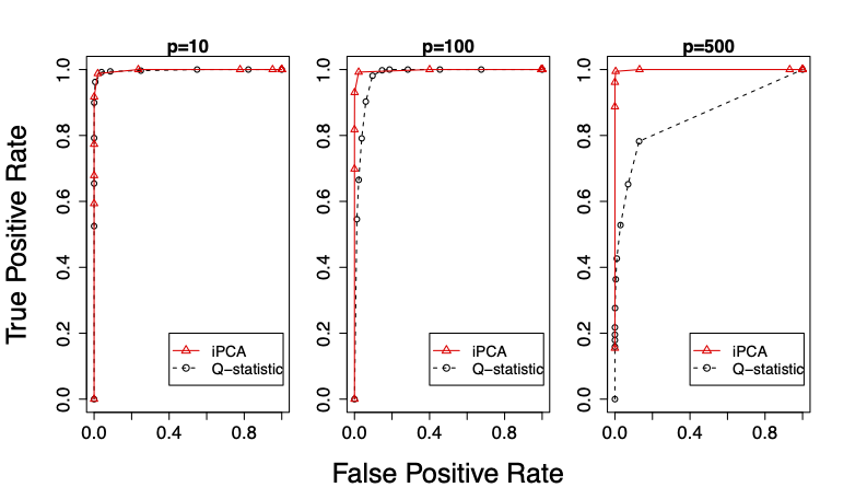
Figure 3: ROC curves of Algorithm 1 (iPCA-based) and Q-statistic for long duration anomaly (6 hour) of low magnitude (snr=2) in synthetic data.

At the same time, the proposed iPCA-based method also has the advantage of providing us with extra information in comparison to the Q-statistic. Indeed, using the individual time/space alerts, one can identify what percentage of individual true positives/false negatives exist in the time/port space. An example of this information is shown on Table II, where the “rows” variables refer to the detection problem and “indiv” variables refer to the identification one. Namely, the “rows” variables are only concerned with temporal events, while the “indiv” variables take into account the spatial structure as well.

TABLE II: Performance of Algorithm 1 on Synthetic Data. Observe the high True Positive Rate (TPR) and low False Positive Rate (FPR) for carefully chosen thresholds $L$.

L	tpr_rows	fpr_rows	tpr_indiv	fpr_indiv
2	1.00	1.00	1.00	1.00
3	1.00	0.92	1.00	0.92
4	1.00	0.11	0.99	0.11
5	1.00	0.00	0.97	0.00
6	1.00	0.00	0.93	0.00
7	1.00	0.00	0.87	0.00
20	0.08	0.00	0.02	0.00

IV-C Application to real-world Darknet data

Finally, we demonstrate the performance of our method on real-world data obtained from the ORION Network Telescope [12]. The dataset spans the entire month of September 2016 and includes the early days of the infamous Mirai botnet [4]. We constructed minute-wise time series for all TCP/UDP ports present in our data that represent the number of unique sources targeting a port at a given time. For the analysis here, we focused on the top-50 ports based on their frequency in the duration of a month. We implement the algorithm on the data by utilizing the calibrated tuning parameters suggested in IV-A3. We use the first 5000 observations, roughly three and a half days, as our burn-in period to initialize the algorithm. Thus, we have a matrix of $43200\times 50$ Darknet data observations.

The selected dataset includes important security incidents. Indeed, as Figure 4 shows, we detect the onset of scanning activities against TCP/2323 (Telnet for IoT) around September 6th that can be attributed to the Mirai botnet. We also detect some interesting ICMP-related activities (that we represent as port-0) towards the end of the month. We are unsure of exactly what malicious acts these activities represent; however, upon payload inspection we found them to be related with some heavy DNS-related scans (payloads with DNS queries were encapsulated in the ICMP payloads).

In Figures 4 and 5, we are looking for large anomalies (snr=7) of long duration (6 hours). Moreover, inspecting the full alert matrix in Figure 5, we observe a few more alerts for anomalies that deserve further investigation. Some of them might be false positives, although there is no definitive “ground truth” in real-world data and all alerts merit some further forensics analysis. The encouraging observations from Figures 4and 5 are that the incidents beknownst to us are revealed, and that the elected hyper-parameters avoid causing the so-called “alert-fatigue” to the analysts. At the same time, the analysts could tune Algorithm 1 to their preferences, and prioritize which alerts to further investigate based on attack severity, duration, number of concurrently affected ports, etc. All this information is readily available from our methodology.

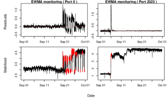
Figure 4: Residuals and detection boundaries (top) and raw traffic (bottom) for ports 0 and 2323. Red color in bottom plots shows the detected anomalies.

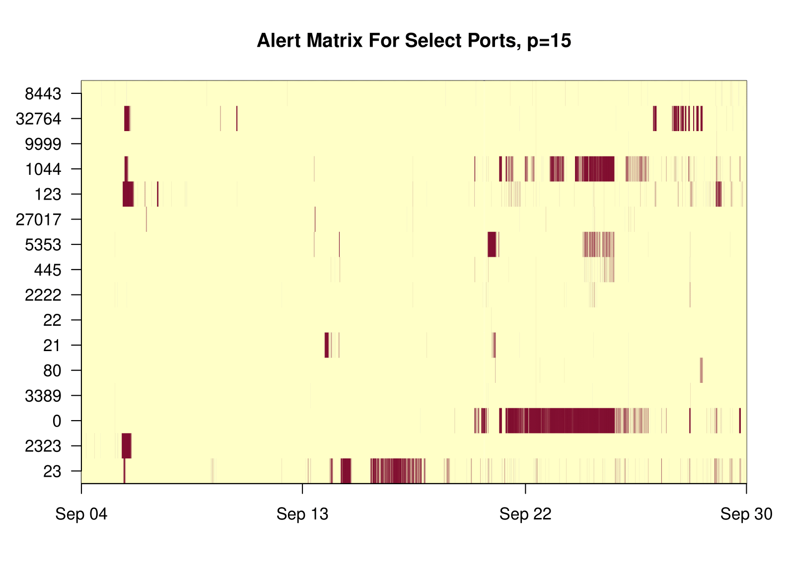
Figure 5: Alert matrix for the Darknet dataset for September 2016 (Mirai onset). Red color indicates detection.

V Appendix

V-A Technical results for Section III

V-A1 Proof for Proposition III.2

We introduce some further notations before we present the proof.

Let ${\bm{b}(j)}$ be the $j$-th column of $B$, $j\in[k]$; ${\bm{b}_{0}(j)}={\bm{b}(j)}/\|{\bm{b}(j)}\|$ the factor loadings normalized; $B_{0}:=[{\bm{b}_{0}(1)},\dots,{\bm{b}_{0}(k)}]$. We shall denote by $\widehat{B}$ and $\widehat{B}_{0}$ the corresponding estimates of $B$ and $B_{0}$ obtained for example by the iPCA algorithm.

For the purpose of the following theoretical results, we shall assume that $\widehat{B}$ and $\widehat{B}_{0}$ are obtained using singular value decomposition of the sample covariance matrix

$$\widehat{\Sigma}:=\frac{1}{n}\sum_{t=1}^{n}{\bm{x}}_{t}{\bm{x}}_{t}^{\top}.$$ (13)

Proof.

Residuals ${\bm{r}}$ from projecting observations onto the space spanned by the first $k$ eigenvectors, are

$${\bm{r}} =(\mathcal{I}_{p}-\mathcal{P}_{\widehat{B_{0}}})(B{\bm{f}}+{\bm{\epsilon}}+{\bm{u}})$$

$$=(\mathcal{I}_{p}-\mathcal{P}_{\widehat{B_{0}}})B{\bm{f}}+(\mathcal{I}_{p}-\mathcal{P}_{\widehat{B_{0}}}){\bm{\epsilon}}+(\mathcal{I}_{p}-\mathcal{P}_{\widehat{B_{0}}}){\bm{u}}$$

or equivalently, we can write

$${\bm{r}}-{\bm{\epsilon}}-{\bm{u}} =\underbrace{(\mathcal{I}_{p}-\mathcal{P}_{\widehat{B_{0}}})B{\bm{f}}}_{I}-\underbrace{\mathcal{P}_{\widehat{B_{0}}}{\bm{\epsilon}}}_{I\!I}-\underbrace{\mathcal{P}_{\widehat{B_{0}}}{\bm{u}}}_{I\!I\!I}$$

We will establish upper bounds on all three terms. The first term,

$${I} =(\mathcal{I}_{p}-\mathcal{P}_{{B_{0}}}+\mathcal{P}_{{B_{0}}}-\mathcal{P}_{\widehat{B_{0}}})B{\bm{f}}$$

$$=(\mathcal{I}_{p}-\mathcal{P}_{{B_{0}}})B{\bm{f}}+(\mathcal{P}_{{B_{0}}}-\mathcal{P}_{\widehat{B_{0}}})B{\bm{f}}$$

$$=-(\mathcal{P}_{\widehat{B_{0}}}-\mathcal{P}_{{B_{0}}})B{\bm{f}}.$$

Using the relationship

$$\|B\|\leq\sqrt{p}\max_{i=1,\ldots,p}\left(\sum_{j=1}^{k}B_{i,j}^{2}\right)^{1/2}$$

and (7) we obtain that $\|B\|\leq\sqrt{pk}C$. By Corollary 1 discussed below,

$${\mathbb{E}}\|(\mathcal{P}_{\widehat{B_{0}}}-\mathcal{P}_{B_{0}})B{\bm{f}}\|\leq{\mathbb{E}}\Big{[}\|(\mathcal{P}_{\widehat{B_{0}}}-\mathcal{P}_{B_{0}})\|\|B\|\|{\bm{f}}\|\Big{]}$$

$$\quad\quad\leq\|B\|\|{\bm{f}}\|\Big{(}{\mathbb{E}}\|\mathcal{P}_{\widehat{B_{0}}}-\mathcal{P}_{B_{0}}\|^{2}\Big{)}^{1/2}$$

$$\quad\quad\leq\sqrt{pk}C\frac{c_{f}\sqrt{k}}{\lambda_{\mathrm{min}}}2\sqrt{k}\left(\mathbb{E}\|\widehat{\Sigma}-\Sigma\|^{2}\right)^{1/2}\;$$

$$\quad\quad\leq\frac{2c_{f}Ck\sqrt{pk}}{\phi(p)}\left(\mathbb{E}\|\widehat{\Sigma}-\Sigma\|^{2}\right)^{1/2}$$ (14)

where we used (6) in the last inequality and which also provides a bound on each coordinate.

For the second term, $I\!I$, decomposed as ${\bm{\epsilon}}-\mathcal{P}_{B_{0}}{\bm{\epsilon}}-(\mathcal{P}_{\widehat{B_{0}}}-\mathcal{P}_{B_{0}}){\bm{\epsilon}}$, notice that $\mathcal{P}_{B_{0}}{\bm{\epsilon}}=B_{0}B_{0}^{\top}{\bm{\epsilon}}\stackrel{{\scriptstyle d}}{{\sim}}B_{0}{\bm{\epsilon}}_{k}$ where ${\mathbb{E}}{\bm{\epsilon}}_{k}=0$ and ${\mathbb{E}}{\bm{\epsilon}}_{k}{\bm{\epsilon}}_{k}^{\top}=I_{k}$. The second moment of the $i$th coordinate is bounded by

$${\mathbb{E}}(\mathcal{P}_{B_{0}}{\bm{\epsilon}})_{i}^{2}={\mathbb{E}}(\sum_{j=1}^{k}B_{0}(i,j)\epsilon_{k}(j))^{2}\leq\frac{kC^{2}}{\lambda_{\mathrm{min}}}$$

because $|B_{0}(i,j)|\leq C/\sqrt{\lambda_{\mathrm{min}}}$. While in $\ell_{2}$ norms, ${\mathbb{E}}\|\mathcal{P}_{B_{0}}{\bm{\epsilon}}\|^{2}={\mathbb{E}}\mathrm{tr}(B_{0}B_{0}^{\top}{\bm{\epsilon}}{\bm{\epsilon}}^{\top}B_{0}B_{0}^{\top})=k$. The last part is controlled similarly as in $I$. Indeed, by the Cauchy-Schwartz inequality, Corollary 1 and (6), we obtain

$$\Big{(}{\mathbb{E}}\|(\mathcal{P}_{\widehat{B_{0}}}-\mathcal{P}_{B_{0}}){\bm{\epsilon}}\|\Big{)}^{2} \leq{\mathbb{E}}\|\mathcal{P}_{\widehat{B_{0}}}-\mathcal{P}_{B_{0}}\|^{2}{\mathbb{E}}\|{\bm{\epsilon}}\|^{2}$$

$$\leq\frac{4k\mathbb{E}\|\widehat{\Sigma}-\Sigma\|^{2}p}{\phi(p)^{2}}.$$

For the third term, we need the von Neumann’s trace inequality: for two matrices $X$ and $Y$, $|\mbox{tr}(XY)|\leq\langle{\bm{\sigma}}(X),{\bm{\sigma}}(Y)\rangle$, where ${\bm{\sigma}}(X)$, ${\bm{\sigma}}(Y)$ are vectors of the singular values of $X$ and $Y$. By Holder inequality, $|\mbox{tr}(XY)|\leq\|{\bm{\sigma}}(X)\|_{1}\|{\bm{\sigma}}(Y)\|_{\infty}=\mbox{tr}(X)\|Y\|$, for real symmetric positive definite matrices.

Decompose $I\!I\!I$ as ${\bm{u}}-\mathcal{P}_{B_{0}}{\bm{u}}-(\mathcal{P}_{\widehat{B_{0}}}-\mathcal{P}_{B_{0}}){\bm{u}}$. The second moment of the $l$-th coordinate

$${\mathbb{E}}(\mathcal{P}_{B_{0}}u)_{l}^{2} ={\mathbb{E}}(\sum_{i=1}^{p}u_{i}\underbrace{(\sum_{j=1}^{k}B_{0}(lj)B_{0}(ij))}_{a_{il}})^{2}$$

$$={\mathbb{E}}(\sum_{i=1}^{p}a_{il}u_{i})^{2}=\mbox{tr}({\bm{a}}_{l}{\bm{a}}_{l}^{\top}{\mathbb{E}}{\bm{u}}{\bm{u}}^{\top})$$

$$\leq\mbox{tr}({\bm{a}}_{l}{\bm{a}}_{l}^{\top})\|\Sigma_{u}\|\leq\frac{k^{2}C^{4}p\|\Sigma_{u}\|}{\lambda_{\mathrm{min}}^{2}},$$

where ${\bm{a}}_{l}=(a_{1l},\dots,a_{pl})^{\top}$, and the last inequality because $|a_{il}|\leq kC^{2}/\lambda_{\mathrm{min}}$. The last part in $I\!I\!I$, again using Corollary 1 and (6), is bounded by

$$({\mathbb{E}}\|(\mathcal{P}_{\widehat{B_{0}}}-\mathcal{P}_{B_{0}}){\bm{u}}\|)^{2} \leq{\mathbb{E}}\|\mathcal{P}_{\widehat{B_{0}}}-\mathcal{P}_{B_{0}}\|^{2}{\mathbb{E}}\mbox{tr}({\bm{u}}{\bm{u}}^{\top})$$

$$\leq\frac{4k{\mathbb{E}}\|\widehat{\Sigma}-\Sigma\|^{2}\mbox{tr}(\Sigma_{u})}{\phi(p)^{2}}$$

Taken together,

$${\mathbb{E}}({\bm{r}}-{\bm{\epsilon}}-{\bm{u}})_{i}^{2}\leq\left[\sqrt{{\mathbb{E}}(I_{i})^{2}}+\sqrt{{\mathbb{E}}(I\!I_{i})^{2}}+\sqrt{{\mathbb{E}}(I\!I\!I_{i})^{2}}\right]^{2}$$

$$\leq\Bigg{[}\frac{2c_{f}Ck\sqrt{pk}}{\phi(p)}\left({\mathbb{E}}\|\widehat{\Sigma}-\Sigma\|^{2}\right)^{1/2}+\frac{2\sqrt{kp}}{\phi(p)}\left({\mathbb{E}}\|\widehat{\Sigma}-\Sigma\|^{2}\right)^{1/2}+$$

$$\frac{\sqrt{k}C}{\phi(p)}+\frac{kC^{2}\sqrt{p}\|\Sigma_{u}\|^{1/2}}{\phi(p)}+\frac{2\sqrt{k}\left({\mathbb{E}}\|\widehat{\Sigma}-\Sigma\|^{2}\right)^{1/2}\sqrt{\mbox{tr}(\Sigma_{u})}}{\phi(p)}\Bigg{]}^{2}$$

$$=\Bigg{[}\left({\mathbb{E}}\|\widehat{\Sigma}-\Sigma\|^{2}\right)^{1/2}\frac{2\sqrt{kp}}{\phi(p)}\left(c_{f}Ck+1+\sqrt{\frac{\mbox{tr}(\Sigma_{u})}{p}}\right)$$

$$+\frac{\sqrt{k}C}{\phi(p)}\left(1+\sqrt{kp}C\|\Sigma_{u}\|^{1/2}\right)\Bigg{]}^{2}.$$

V-A2 Distance between $\Sigma$ and $\hat{\Sigma}$

Looking at Proposition III.2, one can see that we need a bound on

$${\mathbb{E}}\|\widehat{\Sigma}-\Sigma\|^{2}.$$

Recall that the signal $u_{t}$ is assumed random such that

$$\Sigma_{u}:={\mathbb{E}}[u_{t}u_{t}^{\top}],$$

while by (2), $x_{t}=Bf_{t}+u_{t}+\epsilon_{t}.$ Let also $\Sigma_{\epsilon}={\mathbb{E}}[\epsilon\epsilon^{\top}]$ and $\Sigma:=B^{\top}B$.

When we see some data contaminated with sparse anomalies, we can estimate

$$\widehat{\Sigma}=\frac{1}{n}\sum_{t=1}^{n}x_{t}x_{t}^{\top} =\Sigma+B\frac{1}{n}\sum_{t=1}^{n}(f_{t}f_{t}^{\top}-{\cal I}_{k})B^{\top}+\frac{1}{n}\sum_{t=1}^{n}u_{t}u_{t}^{\top}$$

$$+\frac{1}{n}\sum_{t=1}^{n}\epsilon_{t}\epsilon_{t}^{\top}+B\frac{1}{n}\sum_{t=1}^{n}f_{t}(u_{t}+\epsilon_{t})^{\top}$$

$$+\frac{1}{n}\sum_{t=1}^{n}(u_{t}+\epsilon_{t})f_{t}^{\top}B^{\top}$$

$$=:\Sigma+BR_{f}B^{\top}+\hat{\Sigma}_{u}+\hat{\Sigma}_{\epsilon}+BR+R^{\top}B^{\top}$$

$$+\frac{1}{n}\sum_{t=1}^{n}\epsilon_{t}u_{t}^{\top}+\frac{1}{n}\sum_{t=1}^{n}u_{t}\epsilon_{t}^{\top},$$

where

$$R_{f} :=\frac{1}{n}\sum_{t=1}^{n}(f_{t}f_{t}^{\top}-{\cal I}_{k})$$

$$R :=\frac{1}{n}\sum_{t=1}^{n}f_{t}(u_{t}+\epsilon_{t})^{\top}$$

$$\hat{\Sigma}_{\epsilon} :=\frac{1}{n}\sum_{t=1}^{n}\epsilon_{t}\epsilon_{t}^{\top}$$

$$\hat{\Sigma}_{u} :=\frac{1}{n}\sum_{t=1}^{n}u_{t}u_{t}^{\top}.$$

In order to obtain upper bounds on the squared expectation of the operator norm ${\mathbb{E}}[\|\widehat{\Sigma}-\Sigma\|^{2}],$ we will need upper bounds on ${\mathbb{E}}\|R_{f}\|^{2},{\mathbb{E}}[\|\widehat{\Sigma}_{u}\|^{2}]$, ${\mathbb{E}}[\|\widehat{\Sigma}_{\epsilon}\|^{2}]$, ${\mathbb{E}}[\|R\|^{2}]$ and ${\mathbb{E}}\|\frac{1}{n}\sum_{t=1}^{n}\epsilon_{t}u_{t}^{\top}\|^{2}.$

We start with ${\mathbb{E}}\|\hat{\Sigma}_{\epsilon}\|^{2}$ and we assume that $\epsilon_{t}=(\epsilon_{t}(i))_{i=1}^{p},\ t=1,\cdots,n$ is such that $\{\epsilon_{t}(i)\}$ are independent in $i=1,\cdots,p$ but long-range dependent in $t$ zero-mean Gaussian time series. Namely, suppose that

$$C_{\epsilon}(t):={\rm Cov}(\epsilon_{t+s}(i),\epsilon_{s}(i))\sim\sigma^{2}|t|^{2H-2},\ \ \mbox{ as }t\to\infty,$$ (15)

where $H\in(1/2,1)$ is the Hurst long-range dependence parameter of the time-series. Consequently, the auto-covariance $C_{\epsilon}(t)$ is non-summable, i.e.,

$$\sum_{t=0}^{\infty}|C_{\epsilon}(t)|=\infty.$$

We will need the following auxiliary lemma.

Lemma V.1.

Let $C_{n,\epsilon}:=(C_{\epsilon}(t-s))_{n\times n}$, where $C_{\epsilon}$ is as in (15). Then, as $n\to\infty$, we have

$$\|C_{n,\epsilon}\|={\cal O}\Big{(}n^{(2H-1)\vee 1/2}\Big{(}1+1_{\{H=3/4\}}\log(n)\Big{)}\Big{)}$$

Proof.

Using the Cauchy-Schwartz inequality, we obtain that for all $a\in\mathbb{R}^{n}$,

$$\Big{|}\Big{[}C_{n,\epsilon}a\Big{]}(i)\Big{|}\leq\Big{(}\sum_{j=1}^{n}C_{\epsilon}(i-j)^{2}\Big{)}^{1/2}\|a\|.$$

With a standard argument involving the Karamata Theorem and (15), we obtain that

$$\sum_{j=1}^{n}C_{\epsilon}(i-j)^{2} ={\cal O}\Big{(}\sum_{t=1}^{n}t^{4(H-1)}\Big{)}$$

$$={\cal O}\Big{(}n^{4H-3}(1+\log(n)1_{\{H=3/4\}})\Big{)}.$$

This completes the proof. ∎

With this lemma in place, we are now ready to obtain an upper bound on ${\mathbb{E}}\|\hat{\Sigma}_{\epsilon}\|^{2}$.

Lemma V.2.

Let $\epsilon_{t}=(\epsilon_{t}(i))_{i=1}^{p},\ t=1,\cdots,n$ be such that $\epsilon_{t}(i),\ i=1,\cdots,p$ are independent in $i$ zero-mean Gaussian random variables, with their covariance structure satisfying (15). Denote by $C_{n,\epsilon}:=(C_{\epsilon}(t-s))_{n\times n}$ the covariance matrix of the vector $(\epsilon_{t}(1))_{t=1}^{n}$. Let also $\widehat{\Sigma}_{\epsilon}=n^{-1}\sum_{t=1}^{n}\epsilon_{t}\epsilon_{t}^{\top}$. Then,

$$\mathbb{E}\|\hat{\Sigma}_{\epsilon}\|^{2}=O\left(p^{2}\sigma^{4}\right),$$

as $n\to\infty.$

Proof.

Let $E$ be a $p\times n$ matrix whose columns are the $\epsilon_{t}$’s, i.e., $E:=(\epsilon_{1}\,\cdots\,\epsilon_{n})$. Then $\widehat{\Sigma}_{\epsilon}=n^{-1}EE^{\top}$. Notice that the eigenvalues of the matrices $EE^{\top}$ and $E^{\top}E$ are the same and in fact, their largest eigenvalue equals their operator norm with respect to the Euclidean norm. Thus,

$$\|\widehat{\Sigma}_{\epsilon}\|=\sup_{a\not=0}\frac{\|\widehat{\Sigma}_{\epsilon}a\|_{2}}{\|a\|_{2}}=\frac{1}{n}\lambda_{\max}\Big{(}EE^{\top}\Big{)}=\frac{1}{n}\lambda_{\max}\Big{(}E^{\top}E\Big{)},$$

where $\lambda_{\max}:=\lambda_{\max}(EE^{\top})=\lambda_{\max}(E^{\top}E)$ is the largest eigenvalue. Now, however, letting $g_{i}\,i=1,\cdots,p$ denote the columns ot $E^{\top}$, i.e., $g_{i}(t):=\epsilon_{t}(i)$, we get

$$E^{\top}E=\sum_{i=1}^{p}g_{i}g_{i}^{\top},$$

where the $g_{i}$’s are independent in $i$.

Consider the Karhunen-Loéve representation of the $g_{i}$’s, i.e.,

$$g_{i}=\sum_{t=1}^{n}\sqrt{\nu_{n,t}}\varphi_{n,t}Z_{i,t},$$

where $\varphi_{n,t},\ t=1,\cdots,n$ are orthonormal vectors in $\mathbb{R}^{n}$, the $Z_{i,t}$’s are independent standard Normal random variables and $\nu_{n,t},\ t=1,2,\ldots,n$ are the (descending) eigenvalues of $C_{n,\epsilon}.$ Then, letting $a=\sum_{t=1}^{p}a_{t}\varphi_{n,t}$, we obtain

$$\lambda_{\max}^{2} =\sup_{\|a\|_{2}=1}\|E^{\top}Ea\|_{2}^{2}=\sup_{\|a\|_{2}=1}a^{\top}E^{\top}EE^{\top}Ea$$

$$=\sup_{\|a\|_{2}=1}(a^{\top}g_{1},\ldots,a^{\top}g_{p})EE^{\top}\begin{pmatrix}g_{1}^{\top}a\\ \vdots\\ g_{p}^{\top}a\end{pmatrix}$$

$$=\sup_{\|a\|_{2}=1}(a^{\top}g_{1},\ldots,a^{\top}g_{p})(g_{1}^{\top}g_{1}+\ldots+g_{p}^{\top}g_{p})\begin{pmatrix}g_{1}^{\top}a\\ \vdots\\ g_{p}^{\top}a\end{pmatrix}$$

$$=\sup_{\|a\|_{2}=1}\sum_{i=1}^{p}\langle g_{i},g_{i}\rangle\sum_{j=1}^{p}\langle g_{j},a\rangle^{2}.$$

Substituting $a$ and $g_{i}$’s, we have that

$$\lambda_{\max}^{2}(EE^{\top})=\sup_{\|a\|_{2}=1}\sum_{i=1}^{p}\left(\sum_{t=1}^{n}\nu_{n,t}Z_{i,t}^{2}\right)\sum_{j=1}^{p}\left(\sum_{k=1}^{n}\sqrt{\nu_{n,k}}a_{k}Z_{j,k}\right)^{2}.$$

Moving the supremum on the inside, one can get that

$$\|\hat{\Sigma}_{\epsilon}\|^{2} =\frac{1}{n^{2}}\sum_{i=1}^{p}\left(\sum_{t=1}^{n}\nu_{n,t}Z_{i,t}^{2}\right)\sum_{j=1}^{p}\sup_{\|a\|_{2}=1}\left(\sum_{k=1}^{n}\sqrt{\nu_{n,k}}a_{k}Z_{j,k}\right)^{2}$$

$$=:\frac{1}{n^{2}}A\cdot B.$$

Thus, using the Cauchy-Schwarz inequality, we obtain that

$$\mathbb{E}\|\hat{\Sigma}_{\epsilon}\|^{2}\leq\frac{1}{n^{2}}\sqrt{\mathbb{E}A^{2}}\cdot\sqrt{\mathbb{E}B^{2}}$$

For term $A$, one has

$$A =\sum_{i=1}^{p}\left(\sum_{t=1}^{n}\nu_{n,t}Z_{i,t}^{2}\right)$$

$$\stackrel{{\scriptstyle d}}{{=}}\sum_{i=1}^{p}\tilde{\chi}_{i}^{2}\left((\nu_{n,1},\ldots,\nu_{n,n}),(1,1,\ldots,1),(0,0,\ldots 0)\right),$$

where $\tilde{\chi}_{i}^{2}$ are independent generalized chi-squared random variables. So, we have that

$$\mathbb{E}A^{2} ={\rm Var}(A)+(\mathbb{E}A)^{2}=p^{2}\cdot{\rm tr}(C_{n,\epsilon})^{2}+2p\sum_{t=1}^{n}\nu_{n,t}^{2}$$

$$\leq p^{2}\cdot{\rm tr}(C_{n,\epsilon})^{2}+2pn\|C_{n,\epsilon}\|_{\rm op}^{2}.$$

For term $B$ we first look at the supremum. Using Lagrange multipliers, we have that

$$\sup_{\|a\|_{2}=1}\left(\sum_{k=1}^{n}\sqrt{\nu_{n,k}}a_{k}Z_{j,k}\right)^{2}=\sum_{k=1}^{n}\nu_{n,k}Z_{j,k}^{2}$$

which means that

$$B =\sum_{j=1}^{p}\sum_{k=1}^{n}\nu_{n,k}Z_{j,k}^{2}\stackrel{{\scriptstyle d}}{{=}}\sum_{k=1}^{n}\nu_{n,k}\chi_{k}^{2}(p),$$

where we have used the independence of all $Z_{j,k}$ and $\left(\chi_{k}^{2}(p)\right)_{k=1}^{n}$ are independent chi-square random variables with $p$ degrees of freedom. Thus,

$$\mathbb{E}B^{2} =p^{2}{\rm tr}(C_{n,\epsilon})^{2}+2p\sum_{k=1}^{n}\nu_{n,k}^{2}$$

$$\leq p^{2}{\rm tr}(C_{n,\epsilon})^{2}+2pn\|C_{n,\epsilon}\|^{2}.$$

Using the bound from Lemma V.1 and also ${\rm tr}(C_{n,\epsilon})\leq n\cdot\sigma^{2},$ we have that

$$\mathbb{E}\|\hat{\Sigma}_{\epsilon}\|^{2} =O\Big{(}p^{2}\sigma^{4}+2pn^{(2H-2)\vee(-\frac{1}{2})}(1+1_{H=3/4}\log(n))\Big{)}$$

$$=O(p^{2}\sigma^{4}),$$

as $n\to\infty.$ ∎

Finally, we state a bound on the limit $\mathbb{E}\|\widehat{\Sigma}-\Sigma\|^{2}$, assuming that $k$ is fixed or $k=o(p).$

Proposition V.3.

Let $u_{t}$ be long-range dependent with i.i.d. standard normal marginals independent of $\epsilon_{t}$, with its covariance structure $\Sigma_{u}$ satisfying an analogue to Condition (15). Assume also that $\sup_{t}\mathbb{E}\|u_{t}\|_{2}^{2}\leq c_{u},$ and that $\|{\bm{f}}_{t}\|^{2}\leq c_{f}^{2}k,$ $t=1,\ldots,n$. Then,

$$\lim_{n\to\infty}\mathbb{E}\|\widehat{\Sigma}-\Sigma\|^{2} =O\Big{(}p^{4}+p^{3}+p^{2}+p\sqrt{{\rm tr}(\Sigma_{\epsilon}){\rm tr}(\Sigma_{u})}\Big{)}.$$

Proof.

Recall that

$$\widehat{\Sigma} =\Sigma+BR_{f}B^{\top}+\hat{\Sigma}_{u}+\hat{\Sigma}_{\epsilon}+BR+R^{\top}B^{\top}$$

$$+\frac{1}{n}\sum_{t=1}^{n}\epsilon_{t}u_{t}^{\top}+\frac{1}{n}\sum_{t=1}^{n}u_{t}\epsilon_{t}^{\top},$$

where

$$R_{f} =\frac{1}{n}\sum_{t=1}^{n}\left(f_{t}f_{t}^{\top}-{\cal I}_{k}\right)\quad{\rm and}$$

$$R =\frac{1}{n}\sum_{t=1}^{n}f_{t}(u_{t}+\epsilon_{t})^{\top}.$$

By Lemma V.2, we immediately have that

$$\lim_{n\to\infty}\mathbb{E}\|\widehat{\Sigma}_{\epsilon}\|_{\rm op}^{2}=O\left(p^{2}\sigma^{4}\right).$$

For the term $BR_{f}B^{\top},$ we know that $\|B\|\leq\sqrt{pk}C$. Moreover, we have that $\|f_{t}\|_{2}^{2}\leq c_{f}^{2}k$. Thus,

$$\mathbb{E}\|BR_{f}B^{\top}\|^{2} \leq p^{2}k^{2}C^{4}\mathbb{E}\|R_{f}\|^{2}$$

$$\leq p^{2}k^{2}C^{4}\mathbb{E}\left(\frac{1}{n}\sum_{t=1}^{n}\|{\cal I}_{k}-f_{t}f_{t}^{\top}\|\right)^{2}$$

$$\leq p^{2}k^{2}C^{4}(1+c_{f}^{2}k)^{2}.$$

Next, we are looking at $\widehat{\Sigma}_{u}.$ Again by Lemma V.2, we have that $\lim_{n\to\infty}{\mathbb{E}}\|\widehat{\Sigma}_{u}\|^{2}=O(p^{2}\sigma_{u}^{4})$. We now look at the term $BR$. Start with $R$. Then,

$$\|R\| \leq\frac{1}{n}\sum_{t=1}^{n}\|f_{t}\|_{2}\|u_{t}+\epsilon_{t}\|_{2}$$

$$\leq\frac{1}{n}\sqrt{k}c_{f}\sum_{t=1}^{n}\left(\|u_{t}\|_{2}+\|\epsilon_{t}\|_{2}\right)$$

Thus,

$$\mathbb{E}\|BR\|^{2}\leq\frac{1}{n^{2}}pk^{2}C^{2}c_{f}^{2}{\mathbb{E}}\left(\sum_{t=1}^{n}(\|u_{t}\|_{2}+\|\epsilon_{t}\|)\right)^{2}.$$

Looking at the expectation above, and because of the independence of $\epsilon_{t}$ and $u_{t}$, we have

$${\mathbb{E}}\left(\sum_{t=1}^{n}(\|u_{t}\|_{2}+\|\epsilon_{t}\|)\right)^{2} ={\mathbb{E}}\left(\sum_{t=1}^{n}\|\epsilon_{t}\|_{2}\right)^{2}+{\mathbb{E}}\left(\sum_{t=1}^{n}\|u_{t}\|_{2}\right)^{2}$$

$$\qquad+2\sum_{t=1}^{n}{\mathbb{E}}\|\epsilon_{t}\|_{2}\sum_{t=1}^{n}{\mathbb{E}}\|u_{t}\|_{2}.$$

We have the following bounds

$$\mathbb{E}\|\epsilon_{t}\|_{2} \leq\sqrt{{\rm tr}(C_{n,\epsilon}})$$

$$\mathbb{E}\|u_{t}\|_{2} \leq\sqrt{{\rm tr}(C_{n,u}}).$$

Moreover, by Cauchy-Schwarz,

$$\frac{1}{n^{2}}\mathbb{E}\left[\sum_{t=1}^{n}\|\epsilon_{t}\|_{2}\right]^{2} \leq\frac{1}{n^{2}}\mathbb{E}\left[\sum_{t=1}^{n}\|\epsilon_{t}\|_{2}^{2}\right]^{2}=p^{2}+\frac{2p}{n},$$

since $\sum_{t=1}^{n}\|\epsilon_{t}\|_{2}^{2}\sim\chi^{2}(n\cdot p).$ Similarly,

$$\frac{1}{n^{2}}\mathbb{E}\left[\sum_{t=1}^{n}\|u_{t}\|_{2}\right]^{2} \leq p^{2}+\frac{2p}{n},$$

Thus,

$$\lim_{n\to\infty}\mathbb{E}\|BR\|^{2}=O\left(pk^{2}C^{2}c_{f}^{2}\left[2p^{2}+2\sqrt{{\rm tr}(\Sigma_{u}){\rm tr}(\Sigma_{\epsilon})}\right]\right).$$

Finally, for the term $\frac{1}{n}\sum_{t=1}^{n}u_{t}\epsilon_{t}^{\top}$, we use the fact that

$$\|\epsilon_{t}u_{t}^{\top}\|=\max\{u_{t}^{\top}\epsilon_{t},0\}.$$

Then,

$$\mathbb{E}\|\frac{1}{n}\sum_{t=1}^{n}u_{t}\epsilon_{t}^{\top}\|^{2} \leq\frac{1}{n^{2}}\mathbb{E}\left[\sum_{t=1}^{n}\|u_{t}\epsilon_{t}^{\top}\|_{\rm op}\right]^{2}$$

$$\leq\frac{1}{n^{2}}\mathbb{E}\left[\sum_{t=1}^{n}|\epsilon_{t}^{\top}u_{t}|\right]^{2}$$

$$\leq\frac{1}{n^{2}}\mathbb{E}\left[\sum_{t=1}^{n}\|\epsilon_{t}\|_{2}\|u_{t}\|_{2}\right]^{2}$$

$$\leq\frac{1}{n^{2}}\mathbb{E}\sum_{t=1}^{n}\|\epsilon_{t}\|_{2}^{2}\sum_{t=1}^{n}\|u_{t}\|_{2}^{2}$$

$$=\frac{1}{n^{2}}\sum_{t=1}^{n}\mathbb{E}\|\epsilon_{t}\|_{2}^{2}\sum_{t=1}^{n}\mathbb{E}\|u_{t}\|_{2}^{2}$$

$$=\left(p^{2}+2p\right)^{2}.$$

Putting everything together, one has that

$$\lim_{n\to\infty}\mathbb{E}\|\widehat{\Sigma}-\Sigma\|^{2} =O\Big{(}p^{4}+p^{3}+p^{2}+p\sqrt{{\rm tr}(\Sigma_{\epsilon}){\rm tr}(\Sigma_{u})}\Big{)}.$$

∎

∎

V-B Bounds on difference of projection operators

Let $\sigma_{1}\geq\dots\geq\sigma_{k}$ be the singular values of $\widehat{B_{0}}^{\top}B_{0}$. The $k$ dimensional vector $(\cos^{-1}(\sigma_{1}),\dots,\cos^{-1}(\sigma_{k}))$, called the principal angles, are a generalization of the acute angles between two vectors. Let $\Theta(\widehat{B_{0}},B_{0})$ be the $k\times k$ diagonal matrix with $j$th diagonal entry the $j$th principal angle, then a measure of distance between the space spanned by $\widehat{B_{0}}$ and ${B_{0}}$ is $\sin\Theta(\widehat{B_{0}},B_{0})$, where $\sin$ is taken entry-wise.

The following variant of Davis-Kahan theorem [45] provides a bound for the distances between eigenspaces.

Theorem V.4 (Variant of Davis-Kahan sin $\theta$ theorem).

Let $\Sigma,\widehat{\Sigma}\in\mathbb{R}^{p\times p}$ be symmetric, with eigenvalues $\lambda_{1}\geq\ldots\geq\lambda_{p}$ and $\widehat{\lambda}_{1}\geq\ldots\geq\widehat{\lambda}_{p}$ respectively. Fix $1\leq k\leq p$ and assume that $\lambda_{k}-\lambda_{k+1})>0$, where we define $\lambda_{p+1}=-\infty$. Let $V=({\bm{\nu}}_{1},{\bm{\nu}}_{2},\dots,{\bm{\nu}}_{k})\in\mathbb{R}^{p\times k}$ and $\widehat{V}=(\widehat{{\bm{\nu}}}_{1},\widehat{{\bm{\nu}}}_{2},\dots,\widehat{{\bm{\nu}}}_{k})\in\mathbb{R}^{p\times k}$ have orthonormal columns satisfying $\Sigma{\bm{\nu}}_{j}=\lambda_{j}{\bm{\nu}}_{j}$ and $\widehat{\Sigma}\widehat{{\bm{\nu}}}_{j}=\widehat{\lambda}_{j}\widehat{{\bm{\nu}}}_{j}$ for $j=1,2,\dots,k$. Then

$$\|\sin\Theta(\widehat{V},V)\|_{\mathrm{F}}\leq\frac{2{k^{1/2}\|\widehat{\Sigma}-\Sigma\|}}{\lambda_{k}-\lambda_{k+1}}$$

For our purpose, a more meaningful measure of distances between subspaces is the operator norm of the difference of the projections. Let $\mathcal{P}_{\widehat{B_{0}}}$, $\mathcal{P}_{B_{0}}$ be projections onto the column spaces of $\widehat{B_{0}}$ and $B_{0}$ respectively, we have the following

Corollary 1.

Under assumptions (6) and (7) with $\widehat{B}_{0}$, $B_{0}$, $\widehat{\Sigma}$ and $\Sigma$ as defined in (13), we have

$${\mathbb{E}}\|\mathcal{P}_{\widehat{B_{0}}}-\mathcal{P}_{B_{0}}\|^{2}\leq\frac{4k{\mathbb{E}}\|\widehat{\Sigma}-\Sigma\|^{2}}{\lambda_{k}^{2}}.$$ (16)

Proof of Corollary 1 .

It can be shown that the $l_{2}$ operator norm of the difference between two projection matrices $\mathcal{P}_{\widehat{B_{0}}}$ and $\mathcal{P}_{{B_{0}}}$ is determined by the maximum principal angle between the two subspaces (see, e.g. [47] Chapter 5.15). That is,

$$\|\mathcal{P}_{\widehat{B_{0}}}-\mathcal{P}_{{B_{0}}}\|=\sin(\arccos(\sigma_{k}))=\sqrt{1-\sigma_{k}^{2}}.$$

Consequently, we have

$$\|\mathcal{P}_{\widehat{B_{0}}}-\mathcal{P}_{{B_{0}}}\|^{2}\leq\Big{(}\sum_{j=1}^{k}1-\sigma_{j}^{2}\Big{)}=\|\sin\Theta(\widehat{B_{0}},{B_{0}})\|_{\mathrm{F}}^{2}$$ (17)

Then applying Theorem V.4 and using the fact that $\lambda_{k+1}=0$ completes the proof. ∎

V-C Consistency of EWMA updated marginal variance

In this section we present the proof of Proposition III.1.

Let $\{r_{t},\ t\in\mathbb{Z}\}$ be a zero-mean stationary time series, with some correlation structure

$$\rho_{t}={\rm Cor}(r_{t},r_{0})={\rm Cor}(r_{t+h},r_{h}),\ t\in\mathbb{Z},\ \forall h\in\mathbb{Z}.$$

We want to handle the following problem: we want to estimate the unknown variance of $X_{k}$ non-parametrically and show that our estimator is consistent. For the estimation of this variance, we implement an additional EWMA on the squares of the zero-mean stationary series $\{X_{k},\ k\in\mathbb{Z}\}.$ Our proposed estimator is

$$\hat{\sigma}_{t}^{2}=(1-\lambda_{\sigma})\hat{\sigma}_{t-1}^{2}+\lambda_{\sigma}r_{t}^{2}.$$ (18)

To prove the consistency of this estimator, it suffices to show that the following two properties hold

$$\mathbb{E}\left[\hat{\sigma}_{t}^{2}\right] \stackrel{{\scriptstyle\begin{subarray}{c}t\to\infty\\ \lambda_{\sigma}\to 0\end{subarray}}}{{\longrightarrow}}\sigma_{r}^{2}:={\rm Var}(r_{t})$$

$${\rm Var}\left(\hat{\sigma}_{t}^{2}\right) \stackrel{{\scriptstyle\begin{subarray}{c}t\to\infty\\ \lambda_{\sigma}\to 0\end{subarray}}}{{\longrightarrow}}0.$$

Starting with the expectation, we have that

$$\mathbb{E}\left[\hat{\sigma}_{t}^{2}\right] =\sum_{j=0}^{t}\lambda_{\sigma}(1-\lambda_{\sigma})^{j}\mathbb{E}\left[r_{t-j}^{2}\right]=\sigma_{r}^{2}\sum_{j=0}^{t}\lambda_{\sigma}(1-\lambda_{\sigma})^{j}$$

$$=\sigma_{r}^{2}\lambda_{\sigma}\frac{1-(1-\lambda_{\sigma})^{t+1}}{1-(1-\lambda_{\sigma})}=\sigma_{r}^{2}\left(1-(1-\lambda_{\sigma})^{t+1}\right)$$

$$\stackrel{{\scriptstyle t\to\infty}}{{\longrightarrow}}\sigma_{r}^{2},$$

since $0<\lambda_{\sigma}<1$. Here we have used the expression

$$\hat{\sigma}_{t}^{2}=\sum_{j=0}^{t}\lambda_{\sigma}(1-\lambda_{\sigma})^{j}r_{t-j}^{2},$$

since we have a finite horizon on this EWMA.

Our second goal is to show that the variance of $\hat{\sigma}_{t}^{2}$ vanishes. We start by finding an explicit expression of this variance. We have in general that

$${\rm Var}\left(\hat{\sigma}_{t}^{2}\right) ={\rm Var}\left(\sum_{j=0}^{t}\lambda_{\sigma}(1-\lambda_{\sigma})^{j}r_{t-j}^{2}\right)$$

$$=\sum_{j=0}^{t}\lambda_{\sigma}^{2}(1-\lambda_{\sigma})^{2j}{\rm Var}\left(r_{t-j}^{2}\right)$$

$$+\mathop{\sum_{i=0}^{t}\sum_{j=0}^{t}}_{i\neq j}\lambda_{\sigma}^{2}(1-\lambda_{\sigma})^{i+j}{\rm Cov}\left(r_{t-j}^{2},r_{t-i}^{2}\right).$$

We make the following core assumption to continue our calculations.

Assumption V.1.

The process $\{r_{t},\ t\in\mathbb{Z}\}$ is Gaussian.

Using the fact that $\mathbb{E}(r_{t})=0,$ one can immediately obtain that

$${\rm Var}\left(r_{t-j}^{2}\right)=\mathbb{E}\left[r_{t-j}^{4}\right]-\mathbb{E}\left[r_{t-j}^{2}\right]^{2}=3\sigma_{r}^{4}-\sigma_{r}^{4}=2\sigma_{r}^{4}.$$

Now, we need to explore the covariance in the second summand of the above expression. Let

$$\begin{pmatrix}Z_{1}\\ Z_{2}\end{pmatrix}\sim N\left(0,\begin{pmatrix}1&\rho\\ \rho&1\end{pmatrix}\right).$$

We know that

$$Z_{1}\stackrel{{\scriptstyle d}}{{=}}\rho Z_{2}+\sqrt{1-\rho^{2}}Z_{3},$$

where $Z_{2}$ and $Z_{3}$ are independent standard Normal random variables.. Then, we have that

$${\rm Cov}\left(Z_{1}^{2},Z_{2}^{2}\right)$$

$$\quad=\mathbb{E}\left[Z_{1}^{2}Z_{2}^{2}\right]-\mathbb{E}\left[Z_{1}^{2}\right]\cdot\mathbb{E}\left[Z_{2}^{2}\right]=\mathbb{E}\left[Z_{1}^{2}Z_{2}^{2}\right]-1$$

$$\quad=\mathbb{E}\left[\left(\rho^{2}Z_{2}^{2}+(1-\rho^{2})Z_{3}^{2}+2\rho\sqrt{1-\rho^{2}}Z_{2}Z_{3}\right)Z_{2}^{2}\right]]-1$$

$$\quad=3\rho^{2}+(1-\rho^{2})-1=2\rho^{2}.$$

Using the above one immediately has that

$${\rm Var} \left(\hat{\sigma}_{t}^{2}\right)$$

$$=2\sigma_{t}^{4}\sum_{j=0}^{t}\lambda_{\sigma}^{2}(1-\lambda_{\sigma})^{2j}$$

$$\qquad+2\sigma_{r}^{4}\mathop{\sum_{i=0}^{t}\sum_{j=0}^{t}}_{i\neq j}\lambda_{\sigma}^{2}(1-\lambda_{\sigma})^{i+j}\left[{\rm Cor}\left(r_{t-j},r_{t-i}\right)\right]^{2}$$

$$=2\sigma_{r}^{4}\lambda_{\sigma}^{2}\frac{1-\left[(1-\lambda_{\sigma})^{2}\right]^{t+1}}{1-(1-\lambda_{\sigma})^{2}}$$

$$\qquad+2\sigma_{r}^{4}\lambda_{\sigma}^{2}\mathop{\sum_{i=0}^{t}\sum_{j=0}^{t}}_{i\neq j}(1-\lambda_{\sigma})^{i+j}\rho_{i-j}^{2}$$

$$=2\sigma_{r}^{4}\lambda_{\sigma}\cdot\frac{1-\left[(1-\lambda_{\sigma})^{2}\right]^{t+1}}{2-\lambda_{\sigma}}$$

$$\qquad+2\sigma_{r}^{4}\lambda_{\sigma}^{2}\mathop{\sum_{i=0}^{t}\sum_{j=0}^{t}}_{i\neq j}(1-\lambda_{\sigma})^{i+j}\rho_{i-j}^{2},$$

where in the second equality we used the stationarity of $\{r_{t},\ t\in\mathbb{Z}\}.$

We take the limit as $t\to\infty$ in the above expression, and we have that

$$\lim_{t\to\infty}{\rm Var}\left(\hat{\sigma}_{t}^{2}\right) =\frac{2\sigma_{r}^{4}\lambda_{\sigma}}{2-\lambda_{\sigma}}+2\lambda_{\sigma}^{2}\sigma_{r}^{4}\mathop{\sum_{i=0}^{\infty}\sum_{j=0}^{\infty}}_{i\neq j}(1-\lambda_{\sigma})^{i+j}\rho_{i-j}^{2}.$$

We need a condition on $\{\rho_{t},\ t\in\mathbb{Z}\}$ in order to proceed.

We propose the following condition in order to secure the consistency of the variance.

Condition V.1.

Assume that the sequence $\{\rho_{t},\ t\in\mathbb{Z}\}$ is square summable, namely that

$$\sum_{t=-\infty}^{\infty}\rho_{t}^{2}<\infty.$$

Under this condition, we have the following proposition.

Proposition V.5.

Let $\{r_{t},\ t\in\mathbb{Z}\}$ and $\{\hat{\sigma}_{t}^{2},\ t\in\mathbb{Z}\}$ be defined as in the start of Section V-C and (18) respectively. If Condition V.1 holds, then the estimator $\hat{\sigma}_{t}^{2}$ is consistent.

Proof.

The proof is based on the discussion preceding Proposition V.5 and the following. Let

$$A_{t}:=2\lambda_{\sigma}^{2}\sigma_{t}^{4}\mathop{\sum_{i=0}^{t}\sum_{j=0}^{t}}_{i\neq j}(1-\lambda_{\sigma})^{i+j}\rho_{i-j}^{2}.$$

Then

$$A_{t} \leq 2\lambda_{\sigma}^{2}\sigma_{t}^{4}\mathop{\sum_{i=0}^{t}\sum_{j=0}^{t}}(1-\lambda_{\sigma})^{i+j}\rho_{i-j}^{2}$$

$$=2\lambda_{\sigma}^{2}\sigma_{r}^{4}\sum_{v=0}^{2k}(1-\lambda_{\sigma})^{v}\sum_{n=\max\{-t,v-2t\}}^{\min\{t,v\}}\rho_{n}^{2}$$

$$\leq 2\lambda_{\sigma}^{2}\sigma_{r}^{4}\sum_{v=0}^{2t}(1-\lambda_{\sigma})^{v}\sum_{n=-\infty}^{\infty}\rho_{n}^{2}$$

$$\leq 2\lambda_{\sigma}^{2}\sigma_{r}^{4}\sum_{v=0}^{\infty}(1-\lambda_{\sigma})^{v}\sum_{n=-\infty}^{\infty}\rho_{n}^{2}=2\lambda_{\sigma}\sigma_{r}^{4}\sum_{n=-\infty}^{\infty}\rho_{n}^{2},$$

where we have used the change of variables $v=i+j,n=i-j$ in the second equality. Using the relationship

$${\rm Var}\left(\hat{\sigma}_{t}^{2}\right) =2\sigma_{r}^{4}\lambda_{\sigma}\cdot\frac{1-\left[(1-\lambda_{\sigma})^{2}\right]^{t+1}}{2-\lambda_{\sigma}}$$

$$+2\lambda_{\sigma}^{2}\mathop{\sum_{i=0}^{t}\sum_{j=0}^{t}}_{i\neq j}(1-\lambda_{\sigma})^{i+j}\rho_{i-j}^{2},$$

we have that

$${\rm Var}\left(\hat{\sigma}_{t}^{2}\right)\leq\frac{2\sigma_{r}^{4}\lambda_{\sigma}}{2-\lambda_{\sigma}}+2\lambda_{\sigma}\sigma_{r}^{4}\sum_{n=-\infty}^{\infty}\rho_{n}^{2}.$$

Because of Condition V.1, letting $\lambda_{\sigma}\to 0$, we obtain the desired property, namely that ${\rm Var}\left(\hat{\sigma}_{k}^{2}\right)$ vanishes. ∎

References

• [1] J. Czyz, M. Kallitsis, M. Gharaibeh, C. Papadopoulos, M. Bailey, and M. Karir, “Taming the 800 pound gorilla: The rise and decline of NTP DDoS attacks,” in Proceedings of the 2014 Conference on Internet Measurement Conference, 2014.
• [2] C. Rossow, “Amplification Hell: Revisiting Network Protocols for DDoS Abuse,” in Proceedings of the 2014 Network and Distributed System Security (NDSS) Symposium, February 2014.
• [3] M. Kührer, T. Hupperich, C. Rossow, and T. Holz, “Exit from hell? reducing the impact of amplification ddos attacks,” in Proceedings of the 23rd USENIX Conference on Security Symposium, 2014.
• [4] M. Antonakakis, T. April, M. Bailey, M. Bernhard, E. Bursztein, J. Cochran, Z. Durumeric, J. A. Halderman, L. Invernizzi, M. Kallitsis et al., “Understanding the mirai botnet,” in 26th USENIX Security Symposium (USENIX Security 17), 2017.
• [5] B. Krebs, “KrebsOnSecurity Hit With Record DDoS,” https://krebsonsecurity.com/2016/09/krebsonsecurity-hit-with-record-ddos/.
• [6] P. Paganini, “The hosting provider OVH continues to face massive DDoS attacks launched by a botnet composed at least of 150000 IoT devices.” http://securityaffairs.co/wordpress/51726/cyber-crime/ovh-hit-botnet-iot.html.
• [7] N. Perlroth, “Hackers Used New Weapons to Disrupt Major Websites Across U.S.” http://www.nytimes.com/2016/10/22/business/internet-problems-attack.html.
• [8] A. Klopsch, C. Dietrich, and R. Springer, “A detailed look into the Mozi P2P IoT botnet,” https://www.botconf.eu/botconf-2020/schedule/, 2020.
• [9] B. Krebs, “KrebsOnSecurity Hit By Huge New IoT Botnet Meris,” https://krebsonsecurity.com/2021/09/krebsonsecurity-hit-by-huge-new-iot-botnet-meris/, 2021.
• [10] DHS CISA and NCSC, “COVID-19 Exploited by Malicious Cyber Actors,” https://www.cisa.gov/uscert/ncas/alerts/aa20-099a, 2020.
• [11] D. Moore, C. Shannon, G. Voelker, and S. Savage, “Network telescopes: Technical report,” Cooperative Association for Internet Data Analysis (CAIDA), Tech. Rep., Jul 2004.
• [12] Merit Network, Inc., “ORION: Observatory for Cyber-Risk Insights and Outages of Networks,” https://www.merit.edu/initiatives/orion-network-telescope/, 2022.
• [13] R. Pang, V. Yegneswaran, P. Barford, V. Paxson, and L. Peterson, “Characteristics of internet background radiation,” in Proceedings of the 4th ACM SIGCOMM Conference on Internet Measurement, 2004.
• [14] E. Wustrow, M. Karir, M. Bailey, F. Jahanian, and G. Huston, “Internet background radiation revisited,” in Proceedings of the 10th ACM SIGCOMM Conference on Internet Measurement, 2010.
• [15] Z. Gao and S. Stoev, “Fundamental limits of exact support recovery in high dimensions,” Bernoulli, vol. 26, no. 4, pp. 2605 – 2638, 2020.
• [16] ——, Concentration of Maxima and Fundamental Limits in High-Dimensional Testing and Inference, ser. SpringerBriefs in Probability and Mathematical Statistics.   Cham: Springer, 2021.
• [17] R. Arora, A. Cotter, K. Livescu, and N. Srebro, “Stochastic optimization for pca and pls,” in 2012 50th Annual Allerton Conference on Communication, Control, and Computing (Allerton), 2012, pp. 861–868.
• [18] A. Lakhina, M. Crovella, and C. Diot, “Diagnosing network-wide traffic anomalies,” SIGCOMM Comput. Commun. Rev., 2004.
• [19] A. Dainotti, A. King, K. Claffy, F. Papale, and A. Pescapé, “Analysis of a /0; stealth scan from a botnet,” IEEE/ACM Transactions on Networking, vol. 23, no. 2, pp. 341–354, April 2015.
• [20] K. Benson, A. Dainotti, k. Claffy, and E. Aben, “Gaining insight into as-level outages through analysis of internet background radiation,” ser. CoNEXT Student 2012, 2012.
• [21] A. Dainotti, R. Amman, E. Aben, and K. C. Claffy, “Extracting benefit from harm: Using malware pollution to analyze the impact of political and geophysical events on the internet,” SIGCOMM CCR 2012.
• [22] D. Moore, C. Shannon, D. J. Brown, G. M. Voelker, and S. Savage, “Inferring internet denial-of-service activity,” ACM Trans. Comput. Syst.
• [23] M. Jonker, A. King, J. Krupp, C. Rossow, A. Sperotto, and A. Dainotti, “Millions of targets under attack: A macroscopic characterization of the dos ecosystem,” in Proceedings of the 2017 IMC, 2017.
• [24] F. Shaikh, E. Bou-Harb, J. Crichigno, and N. Ghani, “A machine learning model for classifying unsolicited iot devices by observing network telescopes,” in 2018 14th International Wireless Communications and Mobile Computing Conference (IWCMC), 2018, pp. 938–943.
• [25] J. Czyz, K. Lady, S. G. Miller, M. Bailey, M. Kallitsis, and M. Karir, “Understanding IPv6 Internet background radiation,” in IMC 2013, 2013.
• [26] R. Niranjana, V. A. Kumar, and S. Sheen, “Darknet traffic analysis and classification using numerical agm and mean shift clustering algorithm,” SN Computer Science, vol. 1, no. 1, pp. 1–10, 2020.
• [27] T. Ban, L. Zhu, J. Shimamura, S. Pang, D. Inoue, and K. Nakao, “Behavior analysis of long-term cyber attacks in the darknet,” in International Conference on Neural Information Processing, 2012.
• [28] E. Bou-Harb, N.-E. Lakhdari, H. Binsalleeh, and M. Debbabi, “Multidimensional investigation of source port 0 probing,” Digital Investigation, vol. 11, pp. S114–S123, 2014.
• [29] H. Nishikaze, S. Ozawa, J. Kitazono, T. Ban, J. Nakazato, and J. Shimamura, “Large-scale monitoring for cyber attacks by using cluster information on darknet traffic features,” Procedia Computer Science, vol. 53, pp. 175–182, 2015.
• [30] T. Ban, S. Pang, M. Eto, D. Inoue, K. Nakao, and R. Huang, “Towards early detection of novel attack patterns through the lens of a large-scale darknet,” in 2016 Intl IEEE UIC/ATC/ScalCom/CBDCom/IoP/SmartWorld, 2016.
• [31] M. Zakroum, J. François, I. Chrisment, and M. Ghogho, “Monitoring network telescopes and inferring anomalous traffic through the prediction of probing rates,” IEEE Transactions on Network and Service Management, 2022.
• [32] W. Willinger, V. Paxon, and R. Reidi, “Long-range dependence and data network traffic. long-range dependence: Theory and applications, p. doukhan, g. oppenheim and ms taqqu, eds,” 2001.
• [33] J. M. Lucas, M. S. Saccucci, R. V. Baxley, W. H. Woodall, H. D. Maragh, F. W. Faltin, G. J. Hahn, W. T. Tucker, J. S. Hunter, J. F. MacGregor, and T. J. Harris, “Exponentially weighted moving average control schemes: Properties and enhancements,” Technometrics, 1990.
• [34] E. Candes and B. Recht, “Exact matrix completion via convex optimization,” Communications of the ACM, 2012.
• [35] E. J. Candès, X. Li, Y. Ma, and J. Wright, “Robust principal component analysis?” Journal of the ACM (JACM), vol. 58, no. 3, p. 11, 2011.
• [36] H. Xu, C. Caramanis, and S. Sanghavi, “Robust pca via outlier pursuit,” in Advances in Neural Information Processing Systems, 2010.
• [37] Z. Zhou, X. Li, J. Wright, E. Candes, and Y. Ma, “Stable principal component pursuit,” in Information Theory Proceedings (ISIT), 2010 IEEE International Symposium on.   IEEE, 2010, pp. 1518–1522.
• [38] J. Feng, H. Xu, and S. Yan, “Online robust pca via stochastic optimization,” in Advances in Neural Information Processing Systems, 2013.
• [39] Y. I. Ingster, “Minimax detection of a signal for $\ell^{p}_{n}$-balls,” Mathematical Methods of Statistics, vol. 7, no. 4, pp. 401–428, 1998.
• [40] D. Donoho and J. Jin, “Higher Criticism for detecting sparse heterogeneous mixtures,” The Annals of Statistics, vol. 32, no. 3, pp. 962–994, 2004.
• [41] C. Butucea, M. Ndaoud, N. A. Stepanova, and A. B. Tsybakov, “Variable selection with Hamming loss,” The Annals of Statististics, vol. 46, no. 5, pp. 1837–1875, 2018.
• [42] R. Arora, A. Cotter, K. Livescu, and N. Srebro, “Stochastic optimization for pca and pls,” in 2012 50th Annual Allerton Conference on Communication, Control, and Computing (Allerton).   IEEE, 2012, pp. 861–868.
• [43] D. Degras and H. Cardot, “onlinePCA: Online Principal Component Analysis,” https://rdrr.io/cran/onlinePCA/, 2019.
• [44] A. Bjorck, G. H. Golub et al., “Numerical methods for computing angles between linear subspaces,” Mathematics of computation, 1973.
• [45] Y. Yu, T. Wang, and R. J. Samworth, “A useful variant of the davis-kahan theorem for statisticians,” Biometrika, 2015.
• [46] J. Fan, “Test of significance based on wavelet thresholding and neyman’s truncation,” Journal of the American Statistical Association, 1996.
• [47] C. D. Meyer, Matrix analysis and applied linear algebra.   Siam, 2000, vol. 71.